Trend detection by innovative polygon trend analysis for winds and waves

It is known that densely populated coastal areas may be adversely affected as a result of the climate change effects. In this respect, for coastal protection, utilization, and management it is critical to understand the changes in wind speed (WS) and significant wave height (SWH) in coastal areas. Innovative approaches, which are one of the trend analysis methods used as an effective way to examine these changes, have started to be used very frequently in many fields in recent years, although not in coastal and marine engineering. The Innovative Polygon Trend Analysis (IPTA) method provides to observe the one-year behavior of the time series by representing the changes between consecutive months as well as determining the trends in each individual month. It is not also affected by constraints such as data length, distribution type or serial correlation. Therefore, the main objective of this study is to investigate whether using innovative trend methods compared to the traditional methods makes a difference in trends of the climatological variables. For this goal, trends of mean and maximum WS and SWH series for each month at 33 coastal locations in Black Sea coasts were evaluated. Wind and wave parameters WS and SWH were obtained from 42-year long-term wave simulations using Simulating Waves Nearshore (SWAN) model forced by the Climate Forecast System Reanalysis (CFSR). Monthly mean and maximum WS and SWH ​​were calculated at all locations and then trend analyses using both traditional and innovative methods were performed. Low occurrence of trends were detected for mean SWH, maximum SWH, mean WS, and maximum WS according to the Mann-Kendall test in the studied months. The IPTA method detected more trends, such as the decreasing trend of the mean SWH at most locations in May, July and November December. The lowest (highest) values were seen in summer (winter), according to a one-year cycle on the IPTA template for all variables. According to both methods, most of the months showed a decreasing trend for the mean WS at some locations in the inner continental shelf of the southwestern and southeastern Black Sea. The IPTA method can capture most of the trends detected by the Mann-Kendall method, and more missed by the latter method.

1. Introduction

The coastal areas are generally densely populated. The attractiveness of the coasts leads to an increased number of buildings and assets close to the coastline. For example, in 2000, half of the major cities, counting more than 500,000 inhabitants, were located within 50 km of the coastline (UNEP, 2006). Variations in sea level caused by climate change, wave conditions, and storm surges are only a few significant environmental forces that have physical effects along the coast (Camus et al., 2017). Human activities thus stress coastal areas, and the impacts of climate change are expected to worsen the problems that coastal areas are already facing (IPCC, 2013).

The wind speed, the duration of the wind, wind direction, and fetch are the main factors influencing the wave climate in the open ocean. Therefore, the change in the wind pattern directly influences the wave height and period (Bhavithra and Sannasiraj, 2022). Waves combine local wind-sea and swell coming from distant storms (Young, 1999a). Despite being entirely forced by the wind field, the long-term trends of wave height may be affected by low-frequency variability, e.g., an increasing number of cyclones, in the form of a swell contribution (Young, 1999b; Gulev and Grigorieva, 2006). The need for long-term and reliable time series of marine near-surface winds and significant wave height (SWH) is increasing as climate projections require a baseline climatology against which to be compared, and even more so if dynamical models of the sea state are to be included in future coupled climate scenarios (Cavaleri et al., 2012; Dobrynin et al., 2012). There are also more immediate needs for reliable time series of historical wind and wave climates, such as estimates of return values in areas without observational records (Caires and Sterl, 2005; Aarnes et al., 2012; Breivik et al., 2013; Breivik et al., 2014) or decadal trends in wind and wave parameters.

Trend analysis examines whether the direction of increase or decrease in a time series changes over time. There are two types of trend analysis methods: parametric and nonparametric. The parametric approaches are dependent on the assumption that data fit the normal distribution. They are often preferable in trend analysis research since nonparametric methods do not make this assumption (Onyutha, 2016; Akçay et al., 2022). Mann-Kendall, Spearman’s rho, and Sen’s trend slope tests are some examples of nonparametric methods. The Mann-Kendall test is often preferred in trend analysis of hydro-meteorological data (Saplıoğlu et al., 2014; Caloeiro et al., 2018; Ali et al., 2019; Ay, 2020; Şan et al., 2021). It is also frequently used in trend analysis of wave and wind data (Shanas and Kumar, 2015; Akpınar and Bingölbali, 2016; Aydoğan and Ayat, 2018; Meucci et al., 2020; Amarouche et al., 2021). Innovative methods in trend analysis have attracted attention in recent years (Şen, 2012; Şen, 2014; Şen, 2017; Güçlü, 2018; Şen, 2018; Şen et al., 2019; Güçlü et al., 2020; Şen, 2021). The Innovative Trend Analysis (ITA) proposed by Şen (2012) forms the basis of these innovative approaches. In this method, the data is divided into two equal parts. Both half series are sorted in ascending order, and the 45° line is added to the chart. If the scattering points fall above (below) the 45° line, it indicates an increasing (decreasing) trend. If the scattering points are lined up just above the 45° line, there is no change between the first and second half data. Besides, the data can be divided into low, medium, and high groups in this method. The Innovative Polygon Trend Analysis (IPTA) is one of the novel trend methods proposed by Şen et al. (2019). In this method, polygon patterns are obtained using the mean, minimum, maximum, standard deviation and skewness parameters of the data at different time scales (daily, monthly, etc.). In this way, the one-year behavior of the time series is symbolized. This method can obtain information when determining the trend and the magnitude and slope of trend transitions between successive segments (e.g., months). Innovative approaches are frequently used in investigating the trends of hydro-meteorological parameters (Haktanir and Çıtakoğlu, 2014; Ay and Kisi, 2015; Dabanlı et al., 2016; Caloeiro et al., 2018; Sanikhani et al., 2018; Kuriqi et al., 2020; Harkat and Kisi, 2021; Ahmed et al., 2022). However, the use of these methods in investigating the trend of wave parameters is quite limited (Caloeiero et al., 2019; De Leo et al., 2020; De Leo et al., 2021). The ITA procedure recommended by Şen (2012) was applied in these studies. The IPTA method is applied to wave and wind parameters for the first time in this study.

There are various trend analysis studies conducted on the Black Sea (Valchev et al., 2012; Akpınar and Bingölbali, 2016; Divinsky and Kosyan, 2017; Aydoğan and Ayat, 2018; Onea and Rusu, 2019; Çarpar et al., 2020; Divinsky and Kosyan, 2020; Islek et al., 2020; Islek et al., 2021). Valchev et al. (2012) investigated the linear trends of storminess, mean wind speed (WS), mean and total wave energy in the western Black Sea between 1948 and 2010. Akpınar and Bingölbali (2016) determined the long-term changes of SWH and WS in 33 selected locations on the Black Sea based on 31-year (1979-2009) long-term wave simulations using Simulating Waves Nearshore (SWAN) model forced by the Climate Forecast System Re-analysis. Trends for annual mean and maximum WSs and significant wave heights (SWH) were investigated based on the Mann-Kendall test. Divinsky and Kosyan (2017) studied the spatiotemporal variability of the Black Sea wave climate using 37–year (1979–2015) ERA-Interim wind fields. Aydoğan and Ayat (2018) investigated the long-term trends of SWH in the Black Sea, both on a basin average and spatial basis, on an annual and monthly basis using Sen’s slope method and least square linear regression. Divinsky and Kosyan (2020) investigated trends in the average and maximum power of wind seas, swell, and mixed waves using Mann-Kendall test based on the MIKE 21 SW model results for a 40–year (1979–2018) ERA-Interim dataset. Çarpar et al. (2020) spatially investigated the long-term trends of mean and 95% percentile wind speeds in the Black Sea between 1979 and 2016 on a monthly basis with the help of the Mann-Kendall test. Islek et al. (2020) studied the long-term change of wind characteristics (the wind speed, direction, number and duration of storms, and wind power density) using linear regression on the Black Sea with two widely used data sources ERA-Interim and CFSR, spanning 40- year (1979-2018). Islek et al. (2021) determined the long-term trends of mean and maximum SWH, mean wave period, mean wave direction, storm duration, and wave steepness using linear regression for two separate data sets (SWAN simulations forced with the ERA-Interim and NCEP/NCAR) covering the years 1979–2018 on the Black Sea.

As seen from the literature review in the area of ​​interest and the world, trends for winds and waves were not examined using the IPTA method. With the help of polygon graphics in the IPTA method, a new methodology, the annual behavior of the time series can be followed from January to December. This method questions the existence of a trend each month and allows the direction and size of the transitions between months to be determined. It provides the opportunity to make visual comments as well as numerical data. The following are the primary goals of this research:

* To investigate monthly long-term trends of mean and maximum SWH and WS at 33 locations along the Black Sea coast.

* To examine the one-year behavior of the mean and maximum SWH and WS at locations by examining the transitions between months with the IPTA method, which will assess the month-to-month trends and slopes. In this way, to observe seasonal variations through monitoring changes in successive months.

* To compare traditional (Mann-Kendall) with innovative (IPTA) methods.

For the purposes mentioned above, the locations and data in the study carried out by Akpınar and Bingölbali (2016) were preferred and used. The dataset produced by Akpınar and Bingölbali (2016) was extended with SWAN simulations until 2020. After expanding the data, monthly mean and maximum SWH and WS were obtained for 33 locations. Traditional (Mann-Kendall) and the state of the art (IPTA) trend methods were applied for 42-year mean and max WS and SWH for each month, and trends were determined.

2. Materials and methods

2.1. Study area and data used

The deep-water basin, which covers most of the sea, and the coastal shelf are two morphological aspects of the Black Sea. The shelf band in the northwestern section of the sea stretches up to 200 kilometers broad. A 20-kilometer-long continental slope and shelf differentiate the southern and eastern shores. With a maximum depth of 2212 meters, the center part of the Black Sea basin is a relatively flat plain. The depths off the coasts of Crimea and the Caucasus are steadily rising, reaching 500 meters just a few kilometers from the shore (Divinsky and Kosyan, 2020). Thirty-three locations along these coastal regions of the Black Sea were determined within the scope of the study by taking a degree difference between longitudes. Of these 33 locations, nine are in the southeast (1-9), seven in the northeast (10-16), eight in the northwest (17-24), and nine in the southwest (25-33) of the Black Sea. The positions of these locations are shown in Figure 1. Detailed information about the study area and locations can be found in Akpınar and Bingölbali (2016).

FIGURE 1

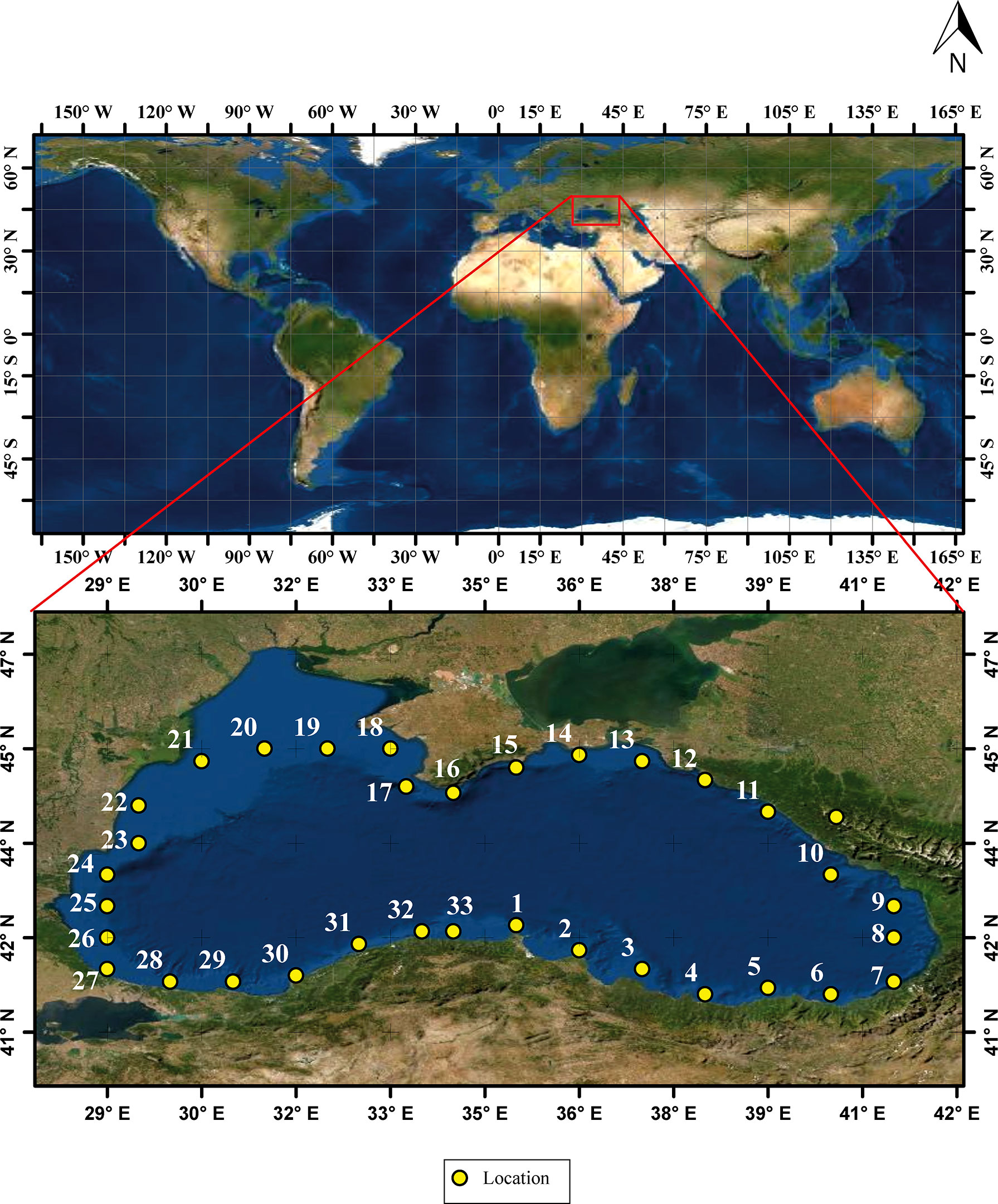
Figure 1 Study area and locations.

2.2. Wave model setup

Forced with CFSR wind fields, SWAN cycle III version 41.01, a third-generation wave model (Booij et al., 1999; Ris et al., 1999), was used to generate and propagate wind waves between 1979 and 2009 by Akpınar and Bingölbali (2016) and extend the dataset until 2020 in the scope of the present study in the Black Sea. Thus, a 42-year long-term wind and wave dataset were formed. The SWAN model was in the third generation and operated in non stationary mode, with a time step of 15 min and one iteration per time step. Akpınar et al. (2012) found this setting to be adequately precise. As for the domain of the model, the entire Black Sea (27°E to 42°E and 40°N to 48°N) was taken into consideration (shown Figure 1). In spherical coordinates, the Black Sea was within a 225×120 regular grid, including the Azov Sea. It has a consistent resolution of 0.067 degrees (1/15°) in both directions, translating into about 7.7 km of latitude and 5.43 km of longitude. Thus, there is 15 cells per latitude and longitude. Thirty-six directional bins and 35 frequency bins were used to discretize the spectrum function of the directional wave variance, which were geometrically positioned from 0.04 Hz to 1.0 Hz. The slightly dispersive BSBT (first-order upwind; backward space, backward time) scheme was used for the numerical scheme. Numerical settings of the SWAN model in the Black Sea were discussed in Akpınar et al. (2012), where the physical settings for the wave model calculations were done with a calibrated SWAN model by Akpınar et al. (2016). The formulation of Komen et al. (1994) was applied for wave growth by wind. 1991b; Janssen’s (1991a) model’s adaptations, where δ=1 according to Rogers et al. (2003), were used for wave energy dissipation by whitecapping. 2016; Akpınar et al. (2015) found that the C_ds=1.5 coefficient for whitecapping dissipation was optimal for the SWAN model forced with the CFSR, so this study used the same. Nonlinear quadruplet interactions were calculated using the Discrete Interaction Approximation (DIA) by Hasselmann et al. (1985), in which λ is 0.25 and C_nl4 is 3×10⁷. A constant for the bottom-friction coefficient (C_fjon=0.038 m² s⁻³) based on JONSWAP was used to evaluate energy dissipation due to bottom friction as advised in Zijlema et al. (2012). The bore model of Battjes and Janssen (1978), in which α is set to 1 and γ is 0.73, was used to model energy dissipation by depth-limited wave breaking. Triad Approximation (LTA) of Eldeberky (1996) was employed to calculate triad wave-wave interactions. The wave model was driven by NOAA, which includes two versions for CFSR winds. Version 1 of the CFS Re-analysis data set (Saha et al., 2010) is available from January 1, 1979, to March 31, 2011. Version 2 (Saha et al., 2014) of the data sets started in March 2011. CFSR wind data sets have a temporal resolution of 1 hour, and they possess a spatial resolution of 0.3125^◦ × 0.3125^◦ from 1979 to 2010 and 0.2045^◦ × 0.2045^◦ from 2011 to the present. With a resolution is 30 arcseconds in both latitude and longitude, the bathymetry shown in Figure 1 was collected from the GEBCO (2014) database. Since currents and water level changes are insignificant to affect the model’s results, they were simply not considered. Parameters like SWH and WS have been saved at a half-hour interval over the entire grid for 42 years. 2016; Akpınar et al. (2015) provide details on the calibration and validation of the SWAN model used.

2.3. Trend analysis

2.3.1. Mann-Kendall test

The Mann-Kendall test is a nonparametric trend analysis tool extensively used. The test statistic S of the method is calculated as (Mann, 1945; Kendall, 1975):

$\begin{array}{ll}S={\displaystyle \sum _{i=1}^{n-1}}{\displaystyle \sum _{j=i+1}^n}sgn\left(x_j-x_i\right)& (1)\end{array}$

where n is the data length, x_i and x_j indicates data values at times i and j, respectively.

$\begin{array}{ll}sgn\left(x_j-x_i\right)=\{\begin{array}{c} 1 ; x_j>x_i\\ 0 ; x_j=x_i\\ -1 ; x_j<x_i\end{array}& (2)\end{array}$

When n>10, the variance of S is calculated as:

$\begin{array}{ll}Var\left(S\right)=\left[n\left(n-1\right)\left(2n+5\right)-{\displaystyle \sum _{i=1}^p}{t}_i\left(t_i-1\right)\left(2t_i+5\right)\right]/18& (3)\end{array}$

In Equation (3), p is the number of tied groups. It means there is equal data in the time series. t_i indicates how many times a data is repeated. Finally, the Z value is obtained from Equation (4):

$\begin{array}{ll}Z=\{\begin{array}{c}\frac{S-1}{\sqrt{Var\left(S\right)}} , S>0 \\ 0 , 0 \\ \frac{S+1}{\sqrt{Var\left(S\right)}} , S<0 \end{array}& (4)\end{array}$

The significance of this test is compared with the standard z value according to the confidence level (90%, 95%, 99%) determined in the standard normal distribution table. If the absolute calculated Z value is greater (less) than the standard z value, there is a significant trend (no trend). In the case of trend, if S is positive (negative), there is an increasing (decreasing) trend.

2.3.2. Innovative polygon trend analysis

Nonparametric tests have some limitations: Mann Kendall and Spearman’s Rho tests are affected by the data length as a result of the simulation studies. As the data length increases, these tests become more powerful (Yue and Wang, 2002; Şen, 2012). In addition, another disadvantage of the Mann-Kendall test is that it accepts serial independence. The presence of serial correlation in a time series showed that the Mann-Kendall test detects trends that do not actually exist (Von Storch, 1995; Şen, 2012). However, Douglas et al. (2000) stated that the prewhitening method, which is used to reduce the serial correlation, will lose some of the existing trend. Contrary to these restrictions, Innovative Trend Analysis (ITA) method proposed by Şen (2012) does not contain any restrictions such as data length, normal distribution fit, and serial correlation removal. The validity of the method was tested by Monte Carlo simulations (Şen, 2012). The IPTA is one of the novel trend methods proposed by Şen et al. (2019). The method has no limitations as it is based on the ITA method. In this method, polygon templates are obtained using the mean, minimum, maximum, standard deviation, and skewness parameters of the data at different time scales (daily, monthly, etc.). If the monthly time scale is preferred, the method is applied as: The monthly values (mean or maximum) of the relevant parameters were divided into two equal groups. In this way, the first half of 42 years of monthly data (21 * 12 = 252 months of data) represent the first group, while 252 months of data for the recent period represent the second group. After that, for each month, the averages (or optionally minimum, maximum, standard deviation, skewness, etc.) of the first half data group (monthly means of the past 21 years) and the second half data group (monthly means of the recent 21 years) were taken and the averages of the first group data were marked on the x-axis and the averages of the second group data were marked on the y-axis, and the 12 points obtained were connected and a polygon was obtained. Finally, the slope and length between two points are obtained by standard formulas. The difference between two months is measured by the line length (transition). The line slope concerning the horizontal axis is known as the trend slope. In the Cartesian coordinate system 1:1 (45°), a straight line divides the diagram into two parts. If scatter points are above (below) the 1:1 line, there is an increasing (decreasing) trend (Şen, 2012). In this method, the measure of significance can be obtained by the relative error percentage (α) between the two half-series (Şen, 2020):

$\begin{array}{ll}\text{α}=100\frac{\left|{\overline{x}}_1-{\overline{x}}_2\right|}{{\overline{x}}_2}& (5)\end{array}$

When α< ± 5%, it is considered that there is no significant trend in the given time series (Şen, 2020).

This approach is a nonparametric method with no assumption. The polygon symbolizes the one-year behavior of the time series. The straight lines connecting the months give information about the changes between months. If the slopes of the straight lines between the months are close, the contribution of the changes between months to the average change in the time series is not significant. The more dynamic and complex a hydro-meteorological event is, the more complex polygons tend to arise.

3. Results

3.1. Mann-Kendall test results

The Mann-Kendall Test results at 95% confidence level for mean and maximum SWH and WS are shown in Figures 2–5, respectively. A significant trend was not observed in approximately 89% of all time series (33 locations x 12 months) of mean SWH (Figure 2). No trends were detected in April, June, July, and October. Increasing trends in March (six locations), August (sixteen locations) and September (ten locations) and decreasing trends in May (five locations) are noteworthy. Trends detected in other months are limited to a few locations. Increasing trends were concentrated in the southeast for March and in the northwest for August and September. Decreasing trends were generally observed at locations in the southwestern part. For the maximum SWH (Figure 3), no trend was observed in any location in February, June, July, and October. There is no trend in approximately 94% of the all time series, but an increasing trend is detected in 5%. Increasing trends were observed in January, August, and September and mostly in locations in the western region.

FIGURE 2

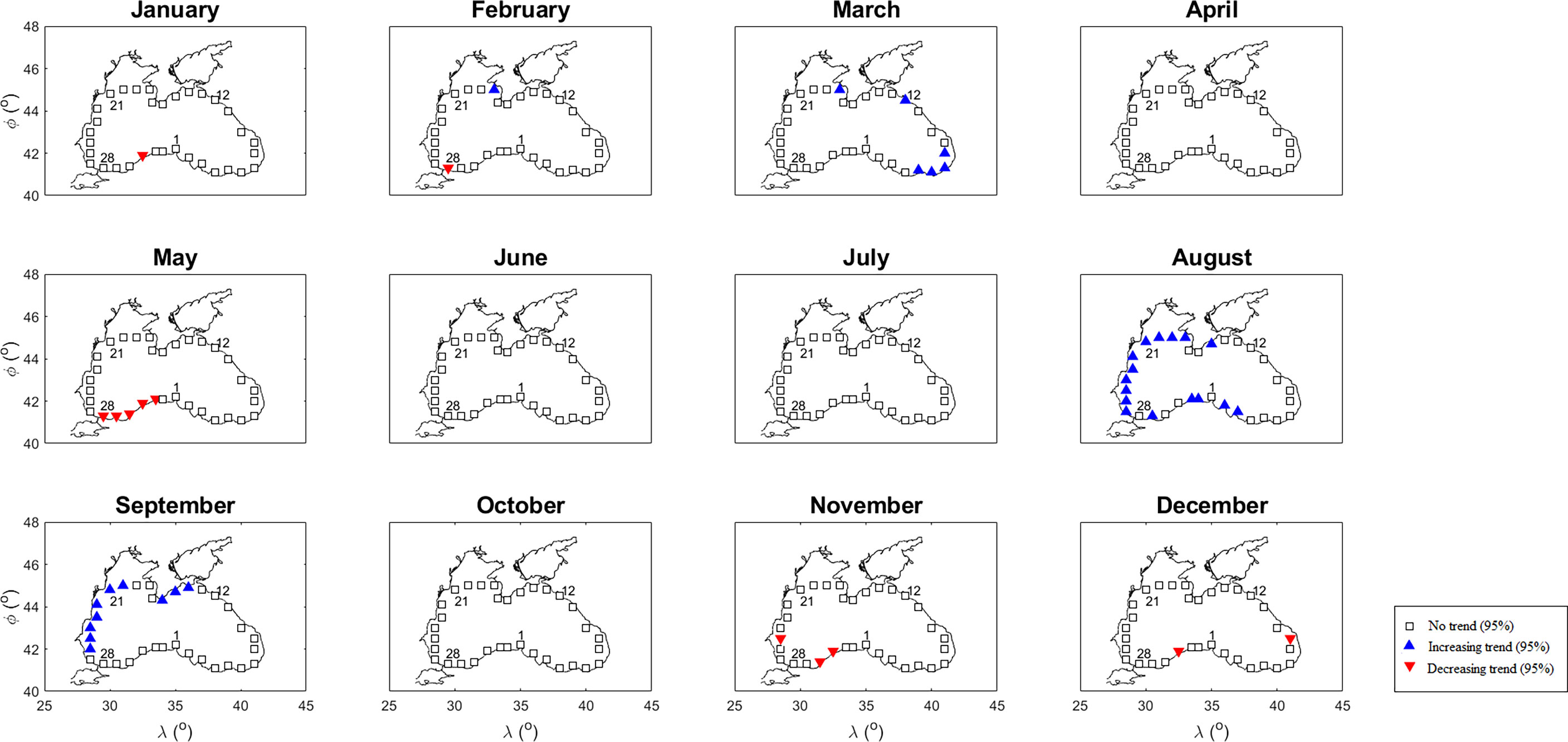
Figure 2 Mann-Kendall results for monthly mean SWHs during 42 years between 1979 and 2020.

FIGURE 3

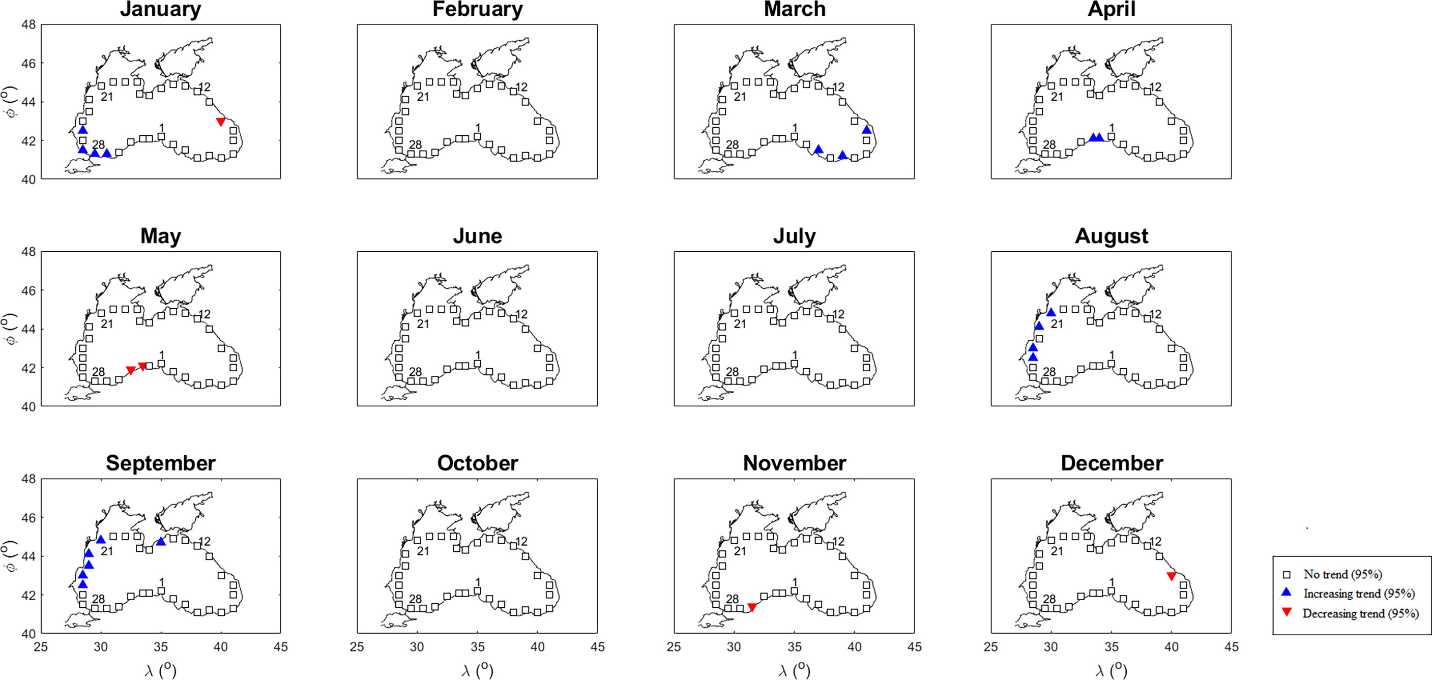
Figure 3 Mann-Kendall results for monthly maximum SWHs during 42 years between 1979 and 2020.

FIGURE 4

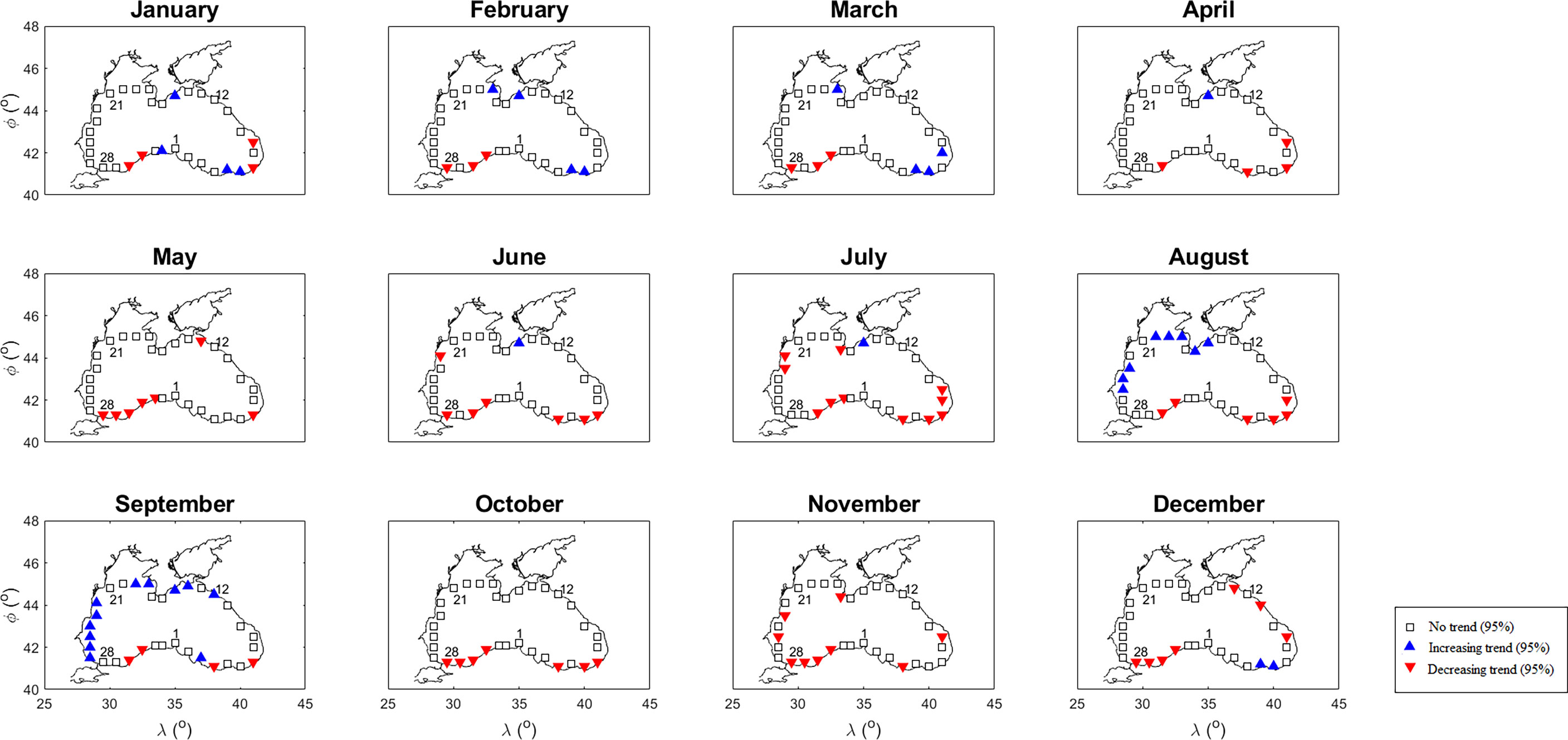
Figure 4 Mann-Kendall results for monthly mean WSs during 42 years between 1979 and 2020.

FIGURE 5

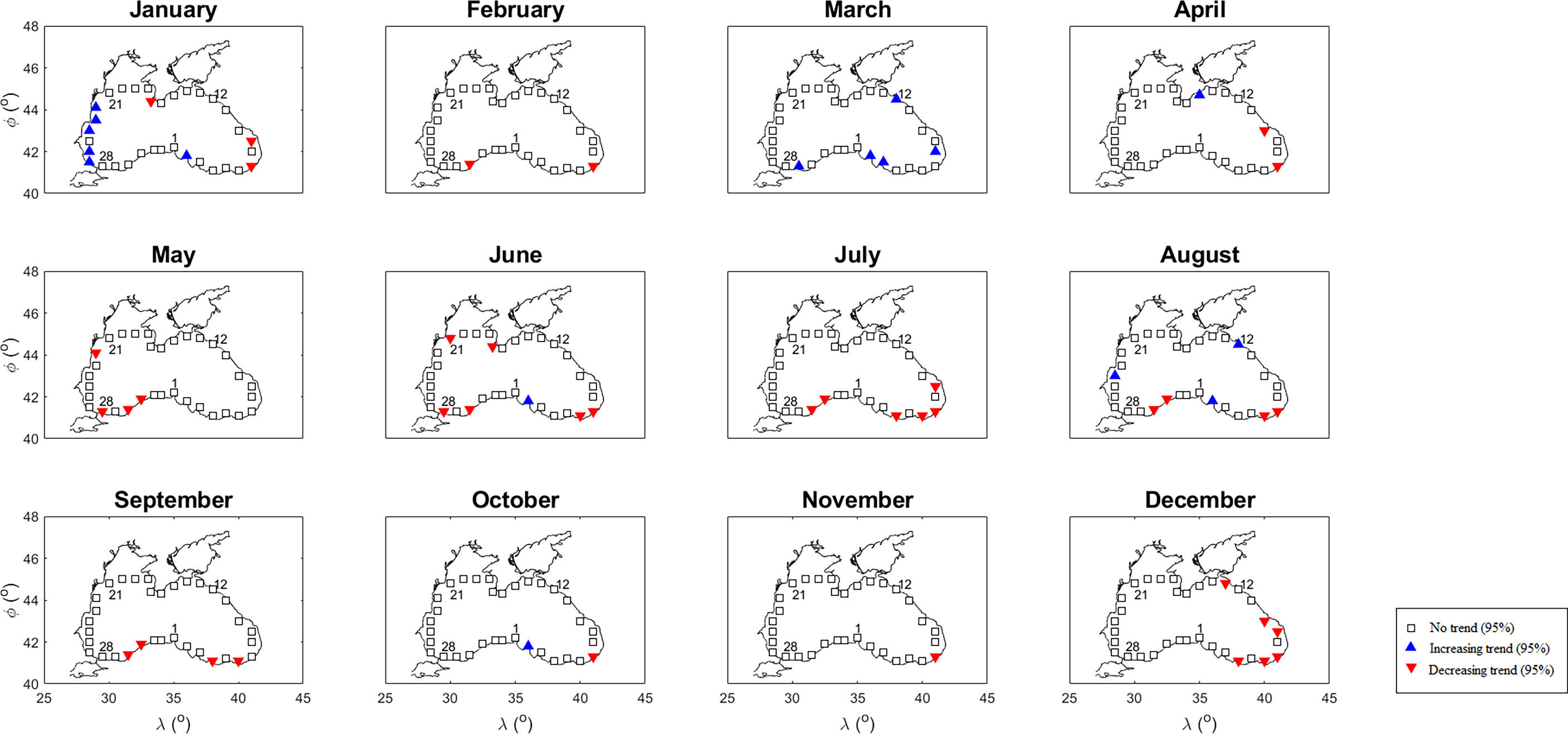
Figure 5 Mann-Kendall results for monthly maximum WSs during 42 years between 1979 and 2020.

Figure 4 presents the monthly Mann-Kendall test results of mean WS. Similar to the mean SWH, increasing trends in the western and northern regions were observed in August and September. A decreasing trend was observed in all months at location 30, located in the southwest. An increasing (decreasing) trend was detected in the winter months (other months) in the some locations belonging to the southeast part where the trend was determined. No significant trends were found in 340 of the 396 (33 locations x 12 months) months (33 locations x 12 months) for maximum WS (Figure 5). In the southeast (west) region, the decreasing (increasing) trends in July and December (January) are noteworthy.

3.2. Innovative polygon trend analysis results

The graphs of the IPTA were obtained for 33 selected locations. A single plot for locations with similar characteristics was presented to provide a summary presentation and ease of review. Results were given for eight locations, two in each of the four identified regions (Figures 6–9). Eight different locations were preferred to evaluate different wind and wave parameters. Trends for the months are seen in the IPTA charts visually. However, when querying the trend assets of the months the relative error percentage (α) between two half series is required to be greater than 5%, as mentioned in the method section 2.3.2. Tables 1–4 are considered a significant trend only in the months that meet this condition. The IPTA graphs for the monthly mean SWH are shown in Figure 6. Significant trends detected in mean SWH are shown in Table 1. While a narrowing polygon structure was observed in the summer months at the locations in the southeast (locations 1-9) region, a wider polygon was encountered in the spring and winter months (Figure 6). The lowest (highest) SWH values ​​are observed in the summer (winter) months when the one-year behavior is examined. Especially the increasing (decreasing) trends in March (November) are stronger in terms of distance to the 45° line. The transitions between February-March-April and October-November-December are large compared to the others. In October, November, and December, the transitions were increasing. They still remained in the decreasing trend region because mean SWH values ​​in the second half were lower than in the first half. Transitions between February–May period show a decrease. At locations 11 and 15 in the northeast region (locations 10-16), a significant increase (decrease) was observed for the mean SWH values in the January-March period (December). In the northwest (locations 17-24) locations, two separate loops were formed for low and high values. Transitions from July to August were from decreasing area to increasing area. A significant decreasing trend was observed for May and July and the October-December period (locations 25-33). The significant decreases in value in the second half of May, July, November, and December caused a complex structure in the transition between the months, with five different polygons. The IPTA graphs between successive months for the monthly maximum SWH were presented in Figure 7. Table 2 shows significant detected trends in maximum SWH. Similar to the mean SWH, the highest (lowest) values ​​were observed in the winter (summer) months for all locations. A wide loop starting from October and ending in March-April was formed at the upper values. Strong increasing (decreasing) trends were observed in March (May) in most locations. For maximum SWH, a complex structure was observed in which more than two loops were formed.

FIGURE 6

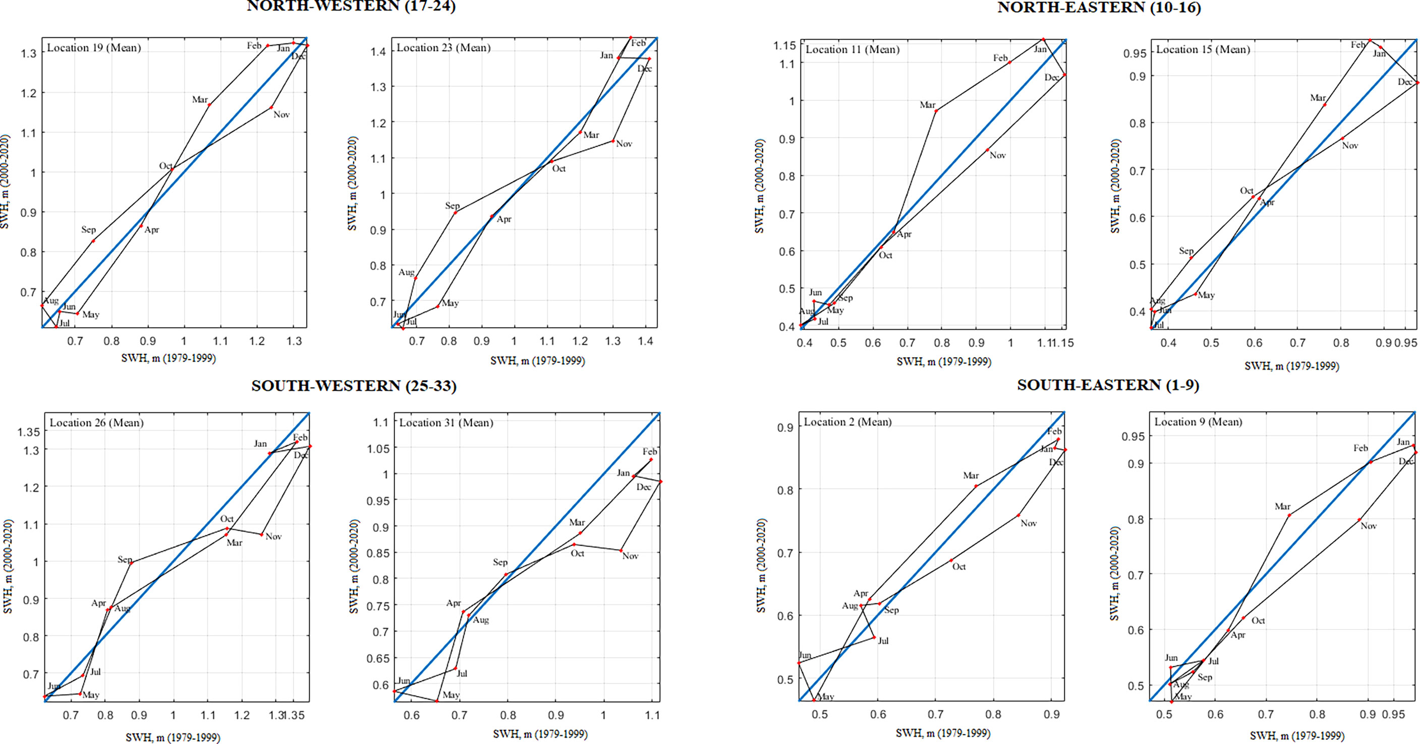
Figure 6 IPTA results for monthly mean SWHs during 42 years between 1979 and 2020.

FIGURE 7

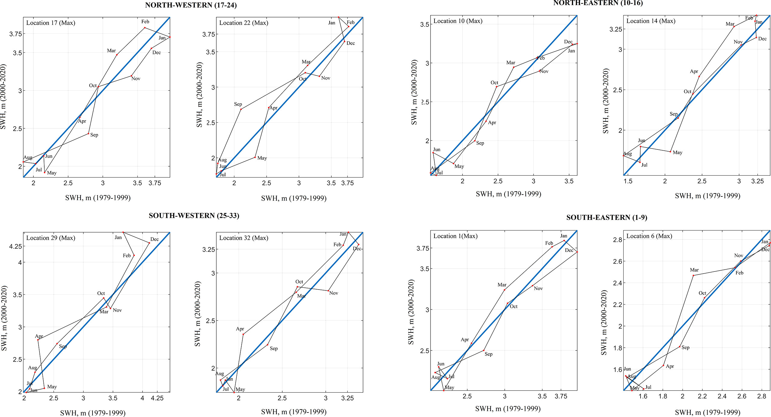
Figure 7 IPTA results for monthly maximum SWHs during 42 years between 1979 and 2020.

FIGURE 8

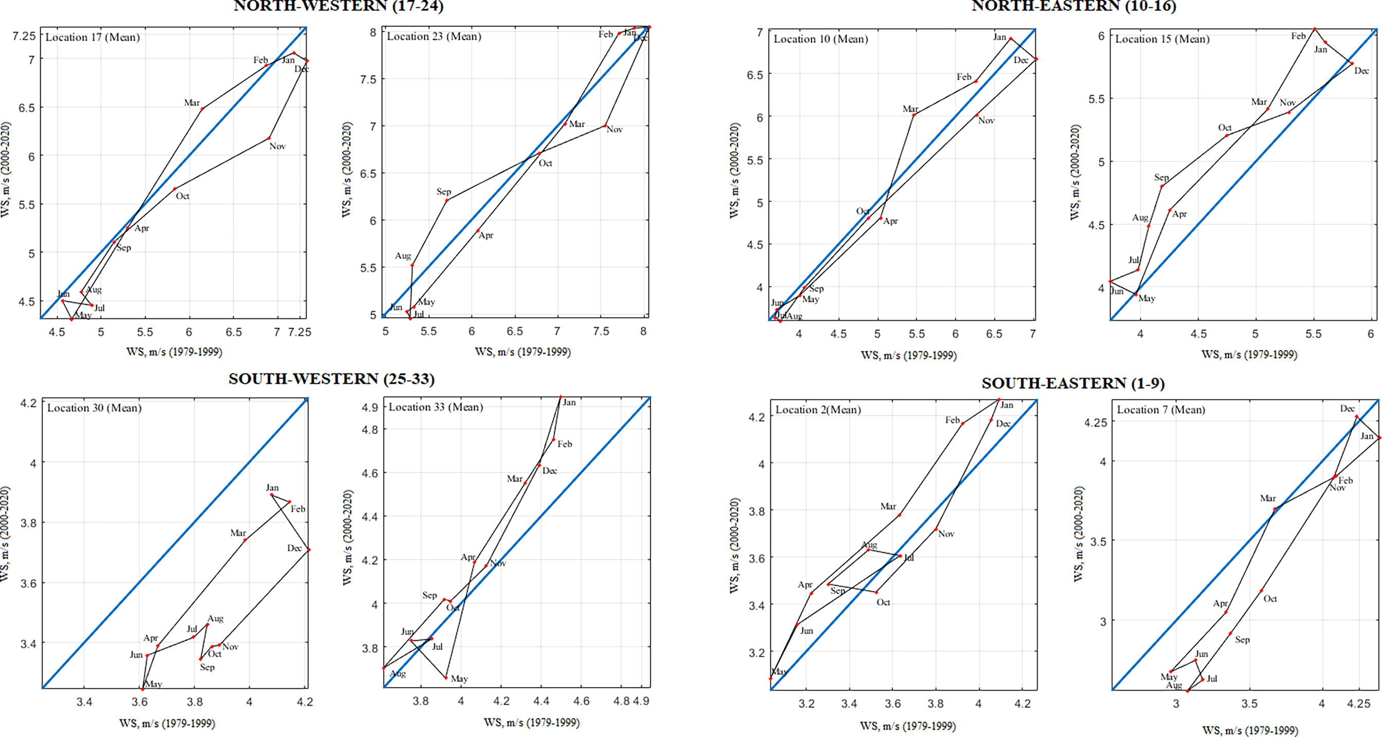
Figure 8 IPTA results for monthly mean WSs during 42 years between 1979 and 2020.

FIGURE 9

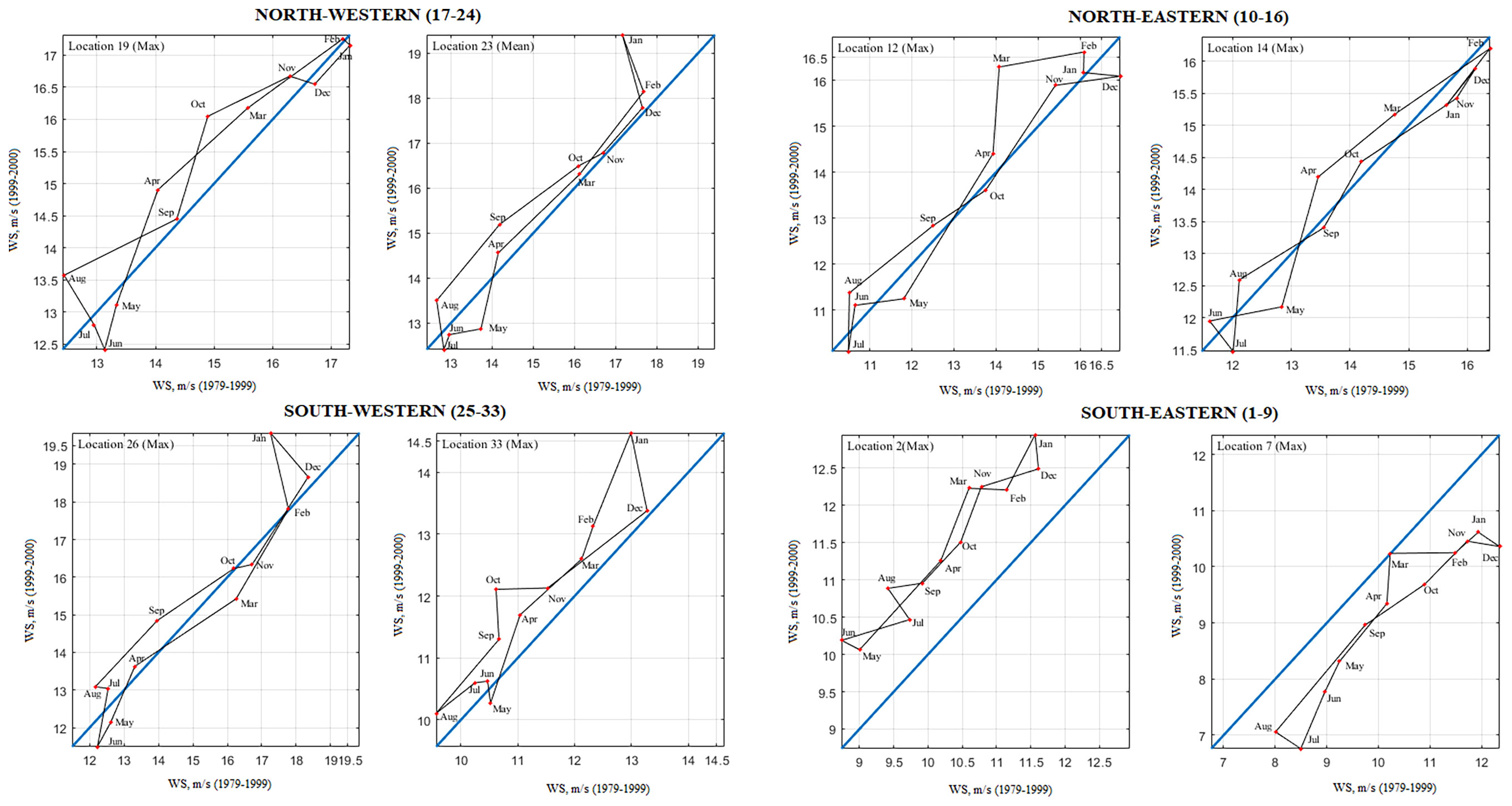
Figure 9 IPTA results for monthly maximum WSs during 42 years between 1979 and 2020.

TABLE 1

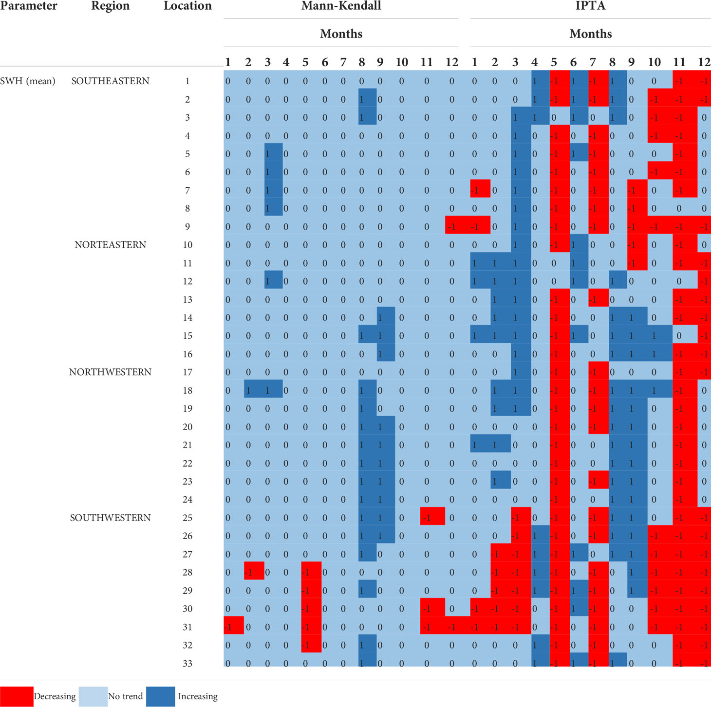
Table 1 Comparison of trend test results from different methods for mean SWH.

TABLE 2

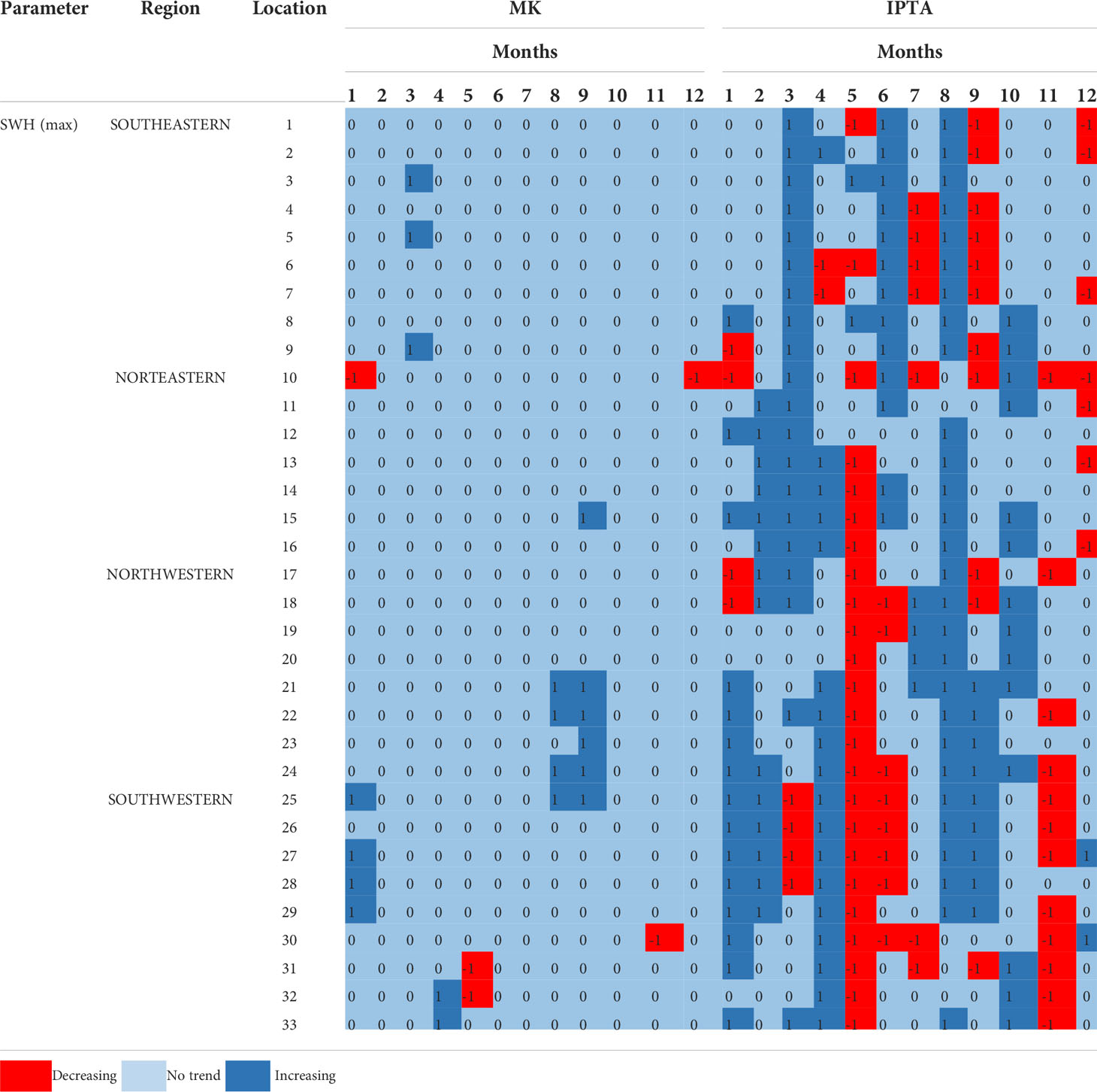
Table 2 Comparison of trend test results from different methods for maximum SWH.

TABLE 3

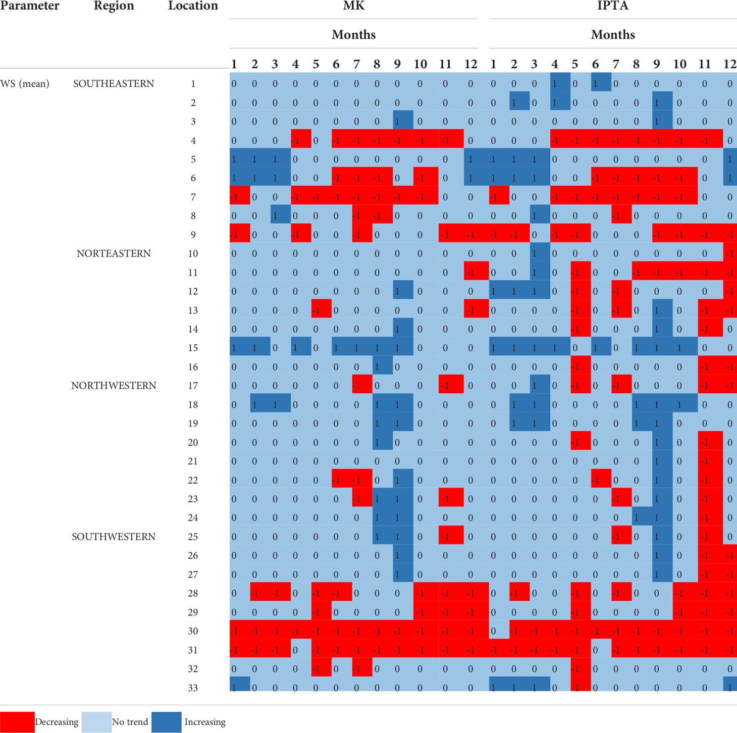
Table 3 Comparison of trend test results from different methods for mean WS.

TABLE 4

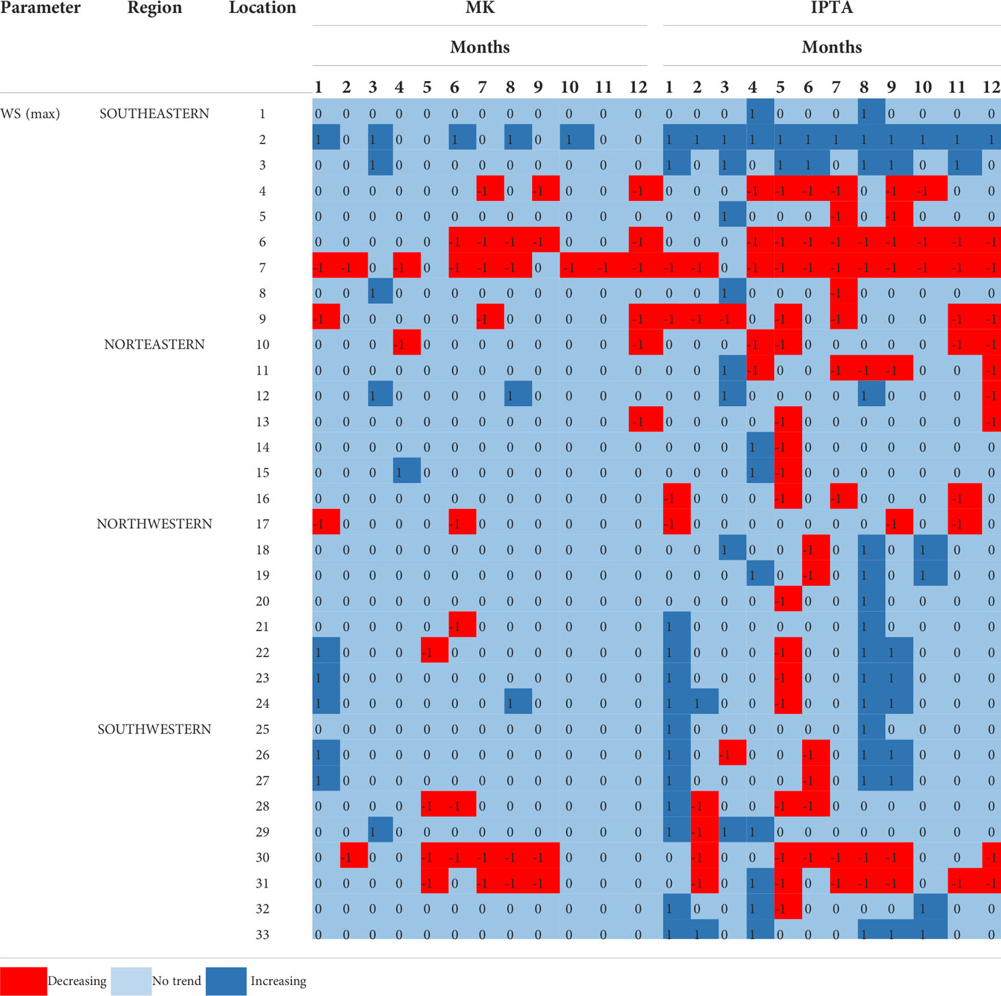
Table 4 Comparison of trend test results from different methods for maximum WS.

IPTA graphs for monthly mean WS were presented in Figure 8. It was observed that the data of the waves in the two locations representing the regions were generally compatible with

each other; this was not the case for the wind data. For example, increases (insignificant) occurred for almost all months in location 2 in the southeast, but a decreasing trend occurred in location 7 in the same region for almost all months. This situation can be seen in Table 3. However, the largest (smallest) mean WS occurred in winter (summer) months, similar to wave data. For high values in the northern locations, loops were seen starting in October and ending at the transition of March-April, but a more complex structure emerged in this range in the south. The transitions between months in the mean WS increase (decrease) from August (January) to December (May). The trend increases at location 15 in the northeast, and decreases in trend at location 30 in the southwest were very severe.

IPTA graphs for monthly maximum WS are presented in Figure 9. There were severe increases (decreases) in maximum WS in location 2 (location 7) in the southeastern part. Table 4 shows that the first three locations 1-3 and the others 4-9 in this region showed opposite trends. As in other wind and wave parameters, high values in maximum WS occurred in winter and low values in summer. The formation of narrower polygons compared to other parameters reveals that the months show similar trend behavior. Transitions between months were in increasing (decreasing) direction between August and December (February and May). In the graphs of the eight stations examined, there are generally increasing trends except for location 7. However it can be seen from Table 4 that the relative error percentage of most of them is less than 5%.

4. Discussion

The monthly analysis findings for mean SWH using the Mann-Kendall test and IPTA were presented in Table 1. The Mann-Kendall test revealed significant trends in 45 of the 396 months (33 locations x 12 months) studied and these results mostly were consistent with the IPTA. In 220 of the 396 months examined, the IPTA approach revealed trends. The IPTA identified a decreasing trend in most locations in May, July, November, and December; the Mann-Kendall test only detected a trend in a small number of locations. The northwestern, where increasing trends were detected in August and September, is where the two approaches produced identical results to a considerable extent. In addition, the decreasing trends measured in May at locations 28-32 in the southwest by the IPTA were also determined by the Mann-Kendall test. The maximum SWHs according to the two methods are presented in Table 2. According to the Mann-Kendall test, increasing (decreasing) trends were seen at 19 (5) months. These trends overlapped very highly with the results obtained in the IPTA.

For mean WS, the percentages of increasing, decreasing, and non-trending months analyzed in the Mann-Kendall test are 9%, 18%, and 73%, respectively (Table 3). The trends observed in this test were also detected by the IPTA. Most of the months showed a decreasing trend according to two methods at locations 4, 7, 28 and 30-31. Decreasing trends in many months at locations 28-31 in the southwest were remarkable according to both methods. In the Mann-Kendall test, no trend was found in most of the months analyzed for maximum WS, whereas an increasing (decreasing) trend was observed in 4% (10%) of the months (Table 4). These trends were also detected by the IPTA.

Considering the findings of the mean and maximum values, there was no 100% agreement for the wave data, and in certain months, contrary patterns were seen (Tables 1, 2). Most locations exhibited an increasing trend for mean and maximum SWH in March and August, but in May, they showed a decreasing trend. The mean and maximum data analysis results were more compatible than the wave data in examining wind data (Tables 3, 4). There was, however, no exact resemblance. Mean and maximum WS showed decreasing trends in most months at locations 4, 7, 9, 30-31. Although there was no 100% agreement between the results of mean winds and waves, the months of March, May, November, and December were typically similar. November showed decreasing trends in most of the locations. Tables 1, 3 also show the months when the mean wind and wave characteristics produced opposite results. The opposite and identical directional results were obtained for the maximum WS and SWH (Tables 2, 4). However, practically all locations, particularly in May, exhibited a decreasing trend in maximum WS and SWH.

A few studies in which parametric and nonparametric methods were applied to waves and winds in the Black Sea, although there is no study in which the IPTA was applied to wave and wind data. Aydoğan and Ayat (2018) investigated the long-term trends of SWH in the Black Sea, both on a basin average and spatial basis, on an annual and monthly basis. Aydoğan and Ayat (2018) detected decreasing trends in the southeast (western) of the Black Sea in July (November) similar to the results of the IPTA method in this study. In May and December, Aydoğan and Ayat (2018) detected significant trends at less than the 90% confidence level in the Black Sea region. In this study, while the Mann-Kendall test detected a trend in very few locations for May and December (95%), the IPTA detected a decreasing trend in most locations. Aydoğan and Ayat (2018) analyzed the MIKE 21 SW model simulations between 1979 and 2016 using the ERA-Interim winds. The present study used SWAN wave model simulations between 1979 and 2020 using CFSR winds. It is therefore estimated that the reason for the inconsistency between the present study and the study performed by Aydoğan and Ayat (2018) for Mann Kendall trend test results may be due to the use of different reanalysis datasets, different physical parameterizations, and numerical settings usage in third-generation models and the difference in data lengths of the wave model used. Çarpar et al. (2020) spatially investigated the long-term trends of monthly mean and 95% percentile WSs in the Black Sea between 1979 and 2016. Results of ERA-Interim and CFSR winds were compared. According to the CFSR, increasing trends were seen in the southeast in March, June, and September. According to Mann-Kendall and IPTA in this study, trends were detected in very few locations for the southeast of the Black Sea in January, February, and March. In September (Çarpar et al., 2020), an increasing trend was determined, especially in the northern and eastern regions, according to the CSFR. This study detected increasing trends, especially in locations 18-27 in September, according to both methods. The reason why this study does not fully agree with Çarpar et al. (2020) may be the different data intervals.

The IPTA approach, according to the findings of this study, can broadly match the trends observed by the Mann-Kendall test. On top of it, the IPTA detected trends in more locations and months; this shows that this new approach to trend analysis is more sensitive. The past studies showed that the IPTA can successfully detect the trends detected by the Mann-Kendall test and give more sensitive results (Şan et al., 2021; Akçay et al., 2022). Innovative graphical ways can provide both visual numerical and verbal comments in addition to trendsetting success. IPTA is a new method in the literature that provides information about trend transitions between successive parts of a time series and determining the trend. No other study applies the IPTA to wave and wind data. By applying this method to mean and maximum wave and wind data, the one-year behavior of these data was observed with the help of polygons. Monthly transitions (January-February, February-March, etc.) were examined, and trends between consecutive months were also discovered. In this way, besides questioning the existence of the trend in the examined months, its relationship with other months was obtained with the help of polygon. In the graphs of the mean SWHs, a polygon structure can be noticed, which narrows in the summer and widens in the spring and winter. The polygon graphs of the maximum SWHs had a more complex structure. The maximum WSs polygon graphs were narrower than the other variables, indicating that the behavior of the months was similar.

5. Conclusions

The results of this study have distinguished IPTA from the Mann-Kendall test, as IPTA detected more trends. The monthly mean and maximum SWH and WS did not show mostly a trend according to the Mann Kendall Test. Besides, the trends detected by the Mann-Kendall test were also caught by the IPTA at a very high rate. Considering the IPTA, in the analysis of mean SWH, the decreasing trends in the May, July, and November-December periods draw attention in most locations. In the analysis of maximum SWHs, most of the stations in the east showed an increasing trend in March, June and August, while all locations in the west showed a decreasing trend in May. Most of the months showed decreasing trends in the mean and maximum WS series at a few eastern locations. Based on a yearly cycle, the lowest (highest) mean SWH was seen in summer (winter); this is also valid for other variables: maximum SWH, average WS, and maximum WS. The transitions between months with the IPTA method showed that there are no temporal shifts, one of the effects of climate change in the meteorological and thus wave events. Wind or wave trends could be different for the same location and month due to distant storms. Significant wind trends in the same locations do not always coincide with SWH trends. This situation may be caused by the main wind direction and the waves that develop in reaction to the wind direction. It is thought that it will be useful to increase the number of locations and also analyze trends of the daily, annual and seasonal mean and maximum wave parameters.

Data availability statement

The data generated during and/or analysed during the current study are available from the corresponding author on reasonable request.

Author contributions

FA: Software, Formal analysis, Visualization, Writing - original draft. BB: Software, Resources, Formal analysis, Visualization, Writing - original draft. AA: Conceptualization, Methodology, Writing - review and editing, Supervision. MK: Conceptualization, Methodology, Writing - review and editing, Supervision. All authors contributed to the article and approved the submitted version.

Acknowledgments

We would like to thank The Scientific and Technological Research Council of Turkey (TUBITAK) for 2211-A Domestic Doctoral Scholarship Program and the Council of Higher Education for 100/2000 Doctoral Scholarship Project for the scholarship they provided to the first author. The authors would like to thank TUBITAK for their support of the previous project with grant number 214M436 because part of the wave data used in the present study was produced within that project.

Conflict of interest

The authors declare that the research was conducted in the absence of any commercial or financial relationships that could be construed as a potential conflict of interest.

Publisher’s note

All claims expressed in this article are solely those of the authors and do not necessarily represent those of their affiliated organizations, or those of the publisher, the editors and the reviewers. Any product that may be evaluated in this article, or claim that may be made by its manufacturer, is not guaranteed or endorsed by the publisher.

References

Aarnes O. J., Breivik Ø., Reistad M. (2012). Wave extremes in the northeast Atlantic. J. Climate 25 (5), 1529–1543. doi: 10.1175/JCLI-D-11-00132.1

CrossRef Full Text | Google Scholar

Ahmed N., Wang G., Booij M. J., Ceribasi G., Bhat M. S., Ceyhunlu A. I., et al. (2022). Changes in monthly streamflow in the hindukush–Karakoram–Himalaya region of Pakistan using innovative polygon trend analysis. Stochastic. Environ. Res. Risk Assess. 36 (3), 811–830. doi: 10.1007/s00477-021-02067-0

CrossRef Full Text | Google Scholar

Akçay F., Kankal M., Şan M. (2022). Innovative approaches to the trend assessment of streamflows in the eastern black Sea basin, Turkey. Hydrolog. Sci. J. 67 (2), 222–247. doi: 10.1080/02626667.2021.1998509

CrossRef Full Text | Google Scholar

Akpınar A., Bekiroğlu S., Van Vledder G. P., Bingölbali B., Jafali H. (2015). Temporal and spatial analysis of wave energy potential during south western coasts of the black Sea. TUBITAK Project 467.

Google Scholar

Akpınar A., Bingölbali B. (2016). Long-term variations of wind and wave conditions in the coastal regions of the black Sea. Nat. Hazards. 84 (1), 69–92. doi: 10.1007/s11069-016-2407-9

CrossRef Full Text | Google Scholar

Akpınar A., Bingölbali B., Van Vledder G. P. (2016). Wind and wave characteristics in the black Sea based on the SWAN wave model forced with the CFSR winds. Ocean. Eng. 126, 276–298. doi: 10.1016/j.oceaneng.2016.09.026

CrossRef Full Text | Google Scholar

Akpınar A., van Vledder G. P., Kömürcü M.İ., Özger M. (2012). Evaluation of the numerical wave model (SWAN) for wave simulation in the black Sea. Continent. Shelf Res. 50, 80–99. doi: 10.1016/j.csr.2012.09.012

CrossRef Full Text | Google Scholar

Ali R., Kuriqi A., Abubaker S., Kisi O. (2019). Long-term trends and seasonality detection of the observed flow in Yangtze river using Mann-Kendall and sen’s innovative trend method. Water 11 (9),1855.

Google Scholar

Amarouche K., Bingölbali B., Akpinar A. (2021). New wind-wave climate records in the Western Mediterranean Sea. Clim. Dyn. 1-24, 1899–1922.

Google Scholar

Ay M. (2020). Trend and homogeneity analysis in temperature and rainfall series in western black Sea region, Turkey. Theor. Appl. Climatol. 139 (3), 837–848. doi: 10.1007/s00704-019-03066-6

CrossRef Full Text | Google Scholar

Aydoğan B., Ayat B. (2018). Spatial variability of long-term trends of significant wave heights in the black Sea. Appl. Ocean. Res. 79, 20–35. doi: 10.1016/j.apor.2018.07.001

CrossRef Full Text | Google Scholar

Ay M., Kisi O. (2015). Investigation of trend analysis of monthly total precipitation by an innovative method. Theor. Appl. Climatol. 120 (3), 617–629. doi: 10.1007/s00704-014-1198-8

CrossRef Full Text | Google Scholar

Battjes J., Janssen J. (1978). Energy loss and set-up due to breaking of random waves. Coast. Eng. Proc. 1 (16), 32. doi: 10.9753/icce.v16.32

CrossRef Full Text | Google Scholar

Bhavithra R. S., Sannasiraj S. A. (2022). Climate change projection of wave climate due to vardah cyclone in the bay of Bengal. Dyn. Atmos. Oceans 97, 101279. doi: 10.1016/j.dynatmoce.2021.101279

CrossRef Full Text | Google Scholar

Booij N., Ris R. C., Holthuijsen L. H. (1999). A third-generation wave model for coastal regions: 1. model description and validation. J. Geophys. Res.: Oceans. 104 (C4), 7649–7666.

Google Scholar

Breivik Ø., Aarnes O. J., Abdalla S., Bidlot J. R., Janssen P. A. (2014). Wind and wave extremes over the world oceans from very large ensembles. Geophys. Res. Lett. 41 (14), 5122–5131. doi: 10.1002/2014GL060997

CrossRef Full Text | Google Scholar

Breivik Ø., Aarnes O. J., Bidlot J. R., Carrasco A., Saetra Ø. (2013). Wave extremes in the northeast Atlantic from ensemble forecasts. J. Climate 26 (19), 7525–7540. doi: 10.1175/JCLI-D-12-00738.1

CrossRef Full Text | Google Scholar

Caires S., Sterl A. (2005). 100-year return value estimates for ocean wind speed and significant wave height from the ERA-40 data. J. Climate 18 (7), 1032–1048. doi: 10.1175/JCLI-3312.1

CrossRef Full Text | Google Scholar

Caloiero T., Aristodemo F., Ferraro D. A. (2019). Trend analysis of significant wave height and energy period in southern Italy. Theor. Appl. Climatol. 138 (1), 917–930. doi: 10.1007/s00704-019-02879-9

CrossRef Full Text | Google Scholar

Caloiero T., Coscarelli R., Ferrari E. (2018). Application of the innovative trend analysis method for the trend analysis of rainfall anomalies in southern Italy. Water Resour. Manage 32 (15), 4971–4983. doi: 10.1007/s11269-018-2117-z

CrossRef Full Text | Google Scholar

Camus P., Losada I. J., Izaguirre C., Espejo A., Menéndez M., Pérez J. (2017). Statistical wave climate projections for coastal impact assessments. Earth's Future 5 (9), 918–933. doi: 10.1002/2017EF000609

CrossRef Full Text | Google Scholar

Çarpar T., Ayat B., Aydoğan B. (2020). Spatio-seasonal variations in long-term trends of offshore wind speeds over the black sea; an inter-comparison of two reanalysis data. Pure Appl. Geophysics. 177 (6), 3013–3037.

Google Scholar

Cavaleri L., Fox-Kemper B., Hemer M. (2012). Wind waves in the coupled climate system. Bull. Am. Meteorolog. Soc. 93 (11), 1651–1661. doi: 10.1175/BAMS-D-11-00170.1

CrossRef Full Text | Google Scholar

Dabanlı İ., Şen Z., Yeleğen M.Ö., Şişman E., Selek B., Güçlü Y. S. (2016). Trend assessment by the innovative-Şen method. Water Resour. Manage 30 (14), 5193–5203. doi: 10.1007/s11269-016-1478-4

CrossRef Full Text | Google Scholar

De Leo F., Besio G., Mentaschi L. (2021). Trends and variability of ocean waves under RCP8. 5 emission scenario in the Mediterranean Sea. Ocean. Dyn. 71 (1), 97–117.

Google Scholar

De Leo F., De Leo A., Besio G., Briganti R. (2020). Detection and quantification of trends in time series of significant wave heights: An application in the Mediterranean Sea. Ocean. Eng. 202, 107155. doi: 10.1016/j.oceaneng.2020.107155

CrossRef Full Text | Google Scholar

Divinsky B. V., Kosyan R. D. (2017). Spatiotemporal variability of the black Sea wave climate in the last 37 years. Continent. Shelf. Res. 136, 1–19. doi: 10.1016/j.csr.2017.01.008

CrossRef Full Text | Google Scholar

Divinsky B. V., Kosyan R. D. (2020). Climatic trends in the fluctuations of wind waves power in the black Sea. Estuarine. Coast. Shelf. Sci. 235, 106577. doi: 10.1016/j.ecss.2019.106577

CrossRef Full Text | Google Scholar

Dobrynin M., Murawsky J., Yang S. (2012). Evolution of the global wind wave climate in CMIP5 experiments. Geophys. Res. Lett. 39 (18), L18606. doi: 10.1029/2012GL052843

CrossRef Full Text | Google Scholar

Douglas E. M., Vogel R. M., Kroll C. N. (2000). Trends in floods and low flows in the united states: impact of spatial correlation. J. hydrology. 240 (1-2), 90–105. doi: 10.1016/S0022-1694(00)00336-X

CrossRef Full Text | Google Scholar

Eldeberky Y. (1996). Nonlinear transformation of wave spectra in the nearshore zone (Ph.D. thesis) (The Netherlands: Delft University of Technology).

Google Scholar

GEBCO (2014). British Oceanographic data centre, centenary edition of the GEBCO digital atlas [CDROM]. (Liverpool: Published on behalf of the Intergovernmental Oceanographic Commission and the International Hydrographic Organization).

Google Scholar

Güçlü Y. S. (2018). Alternative trend analysis: half time series methodology. Water Resour. Manage. 32 (7), 2489–2504.

Google Scholar

Güçlü Y. S., Şişman E., Dabanlı İ. (2020). Innovative triangular trend analysis. Arabian. J. Geosci. 13 (1), 1–8.

Google Scholar

Gulev S. K., Grigorieva V. (2006). Variability of the winter wind waves and swell in the north Atlantic and north pacific as revealed by the voluntary observing ship data. J. Climate 19 (21), 5667–5685. doi: 10.1175/JCLI3936.1

CrossRef Full Text | Google Scholar

Haktanir T., Citakoglu H. (2014). Trend, independence, stationarity, and homogeneity tests on maximum rainfall series of standard durations recorded in Turkey. J. Hydrolog. Eng. 19 (9), 05014009. doi: 10.1061/(ASCE)HE.1943-5584.0000973

CrossRef Full Text | Google Scholar

Harkat S., Kisi O. (2021). Trend analysis of precipitation records using an innovative trend methodology in a semi-arid Mediterranean environment: Cheliff watershed case (Northern Algeria). Theor. Appl. Climatol. 144 (3), 1001–1015. doi: 10.1007/s00704-021-03520-4

CrossRef Full Text | Google Scholar

Hasselmann S., Hasselmann K., Allender J. H., Barnett T. P. (1985). Computations and parameterizations of the nonlinear energy transfer in a gravity-wave spectrum. part II: Parameterizations of the nonlinear energy transfer for application in wave models. J. Phys. Oceanogr. 15, 1378–1391. doi: 10.1175/1520-0485(1985)015<1378:CAPOTN>2.0.CO;2

CrossRef Full Text | Google Scholar

IPCC (2013). “Summary for policymakers. in: Climate change 2013: The physical science basis. contribution of working group I to the fifth assessment report of the intergovernmental panel on climate change, Climate change 2013: The physical science basis”. Eds. Stocker T. F., Qin D., Plattner G.-K., Tignor M., Allen S. K., Boschung J., Nauels A., Xia Y., Bex V., Midgley P. M. (Cambridge, United Kingdom and New York, NY, USA: Cambridge University Press), 1–30. doi: 10.1017/CBO9781107415324.004

CrossRef Full Text | Google Scholar

Islek F., Yuksel Y., Sahin C. (2020). Spatiotemporal long-term trends of extreme wind characteristics over the black Sea. Dyn. Atmospheres. Oceans. 90, 101132. doi: 10.1016/j.dynatmoce.2020.101132

CrossRef Full Text | Google Scholar

Islek F., Yuksel Y., Sahin C., Guner H. A. A. (2021). Long-term analysis of extreme wave characteristics based on the SWAN hindcasts over the black Sea using two different wind fields. Dyn. Atmospheres. Oceans. 94, 101165. doi: 10.1016/j.dynatmoce.2020.101165

CrossRef Full Text | Google Scholar

Janssen P. A. (1991a). “Consequences of the effect of surface gravity waves on the mean air flow,” in Breaking waves (Berlin, Heidelberg: Springer), 193–198.

Google Scholar

Janssen P. A. (1991b). Quasi-linear theory of wind-wave generation applied to wave forecasting. J. Phys. Oceanogr. 21 (11), 1631–1642. doi: 10.1175/1520-0485(1991)021<1631:QLTOWW>2.0.CO;2

CrossRef Full Text | Google Scholar

Kendall M. G. (1975). Rank correlation methods. (London: Charless Griffin).

Google Scholar

Komen G. J., Cavaleri L., Donelan M., Hasselmann K., Hasselmann S., Janssen P. A. E. M. (1994). Dyn. and modelling of ocean waves (Cambridge: Cambridge University Press), 554.

Google Scholar

Kuriqi A., Ali R., Pham Q. B., Gambini J. M., Gupta V., Malik A., et al. (2020). Seasonality shift and streamflow flow variability trends in central India. Acta Geophysica. 68 (5), 1461–1475. doi: 10.1007/s11600-020-00475-4

CrossRef Full Text | Google Scholar

Mann H. B. (1945). Nonparametric tests against trend. Econometrica: J. Econometric. Soc. 13, 245–259. doi: 10.2307/1907187

CrossRef Full Text | Google Scholar

Meucci A., Young I. R., Aarnes O. J., Breivik Ø. (2020). Comparison of wind speed and wave height trends from twentieth-century models and satellite altimeters. J. Climate 33 (2), 611–624. doi: 10.1175/JCLI-D-19-0540.1

CrossRef Full Text | Google Scholar

Onea F., Rusu L. (2019). Long-term analysis of the black sea weather windows. J. Mar. Sci. Eng. 7 (9), 303. doi: 10.3390/jmse7090303

CrossRef Full Text | Google Scholar

Onyutha C. (2016). Identification of sub-trends from hydro-meteorological series. Stochastic. Environ. Res. Risk Assess. 30 (1), 189–205. doi: 10.1007/s00477-015-1070-0

CrossRef Full Text | Google Scholar

Ris R. C., Holthuijsen L. H., Booij N. (1999). A third-generation wave model for coastal regions: 2. verification. J. Geophy. Res.: Oceans. 104 (C4), 7667–7681.

Google Scholar

Rogers W. E., Hwang P. A., Wang D. W. (2003). Investigation of wave growth and decay in the SWAN model: three regional-scale applications. J. Phys. Oceanogr. 33 (2), 366–389. doi: 10.1175/1520-0485(2003)033<0366:IOWGAD>2.0.CO;2

CrossRef Full Text | Google Scholar

Şan M., Akçay F., Linh N. T. T., Kankal M., Pham Q. B. (2021). Innovative and polygonal trend analyses applications for rainfall data in Vietnam. Theor. Appl. Climatol. 144 (3), 809–822.

Google Scholar

Şen Z. (2012). Innovative trend analysis methodology. J. Hydrologic. Eng. 17 (9), 1042–1046.

Google Scholar

Şen Z. (2014). Trend identification simulation and application. J. Hydrologic. Eng. 19 (3), 635–642.

Google Scholar

Şen Z. (2017). Innovative trend significance test and applications. Theor. Appl. Climatol. 127 (3-4), 939–947.

Google Scholar

Şen Z. (2018). Crossing trend analysis methodology and application for Turkish rainfall records. Theor. Appl. Climatol. 131 (1), 285–293.

Google Scholar

Şen Z. (2020). Up-to-date statistical essentials in climate change and hydrology: a review. Int. J. Global Warming 22 (4), 392–431.

Google Scholar

Şen Z. (2021). Conceptual monthly trend polygon methodology and climate change assessments. Hydrolog. Sci. J. 66 (3), 503–512.

Google Scholar

Şen Z., Şişman E., Dabanli I. (2019). Innovative polygon trend analysis (IPTA) and applications. J. Hydrology. 575, 202–210. doi: 10.1016/j.jhydrol.2019.05.028

CrossRef Full Text | Google Scholar

Saha S., Moorthi S., Pan H. L., Wu X., Wang J., Nadiga S., et al. (2010). The NCEP climate forecast system reanalysis. Bull. Am. Meteorolog. Soc. 91 (8), 1015–1058. doi: 10.1175/2010BAMS3001.1

CrossRef Full Text | Google Scholar

Saha S., Moorthi S., Wu X., Wang J., Nadiga S., Tripp P., et al. (2014). The NCEP climate forecast system version 2. J. Clim. 27 (6), 2185–2208. doi: 10.1175/JCLI-D-12-00823.1

CrossRef Full Text | Google Scholar

Sanikhani H., Kisi O., Mirabbasi R., Meshram S. G. (2018). Trend analysis of rainfall pattern over the central India during 1901–2010. Arabian. J. Geosci. 11 (15), 1–14. doi: 10.1007/s12517-018-3800-3

CrossRef Full Text | Google Scholar

Saplıoğlu K., Kilit M., Yavuz B. K. (2014). Trend analysis of streams in the western mediterranean basin of Turkey. Fresenius Environ. Bull. 23 (1), 313–327.

Google Scholar

Shanas P. R., Kumar V. S. (2015). Trends in surface wind speed and significant wave height as revealed by ERA-interim wind wave hindcast in the central bay of Bengal. Int. J. Climatol. 35 (9), 2654–2663. doi: 10.1002/joc.4164

CrossRef Full Text | Google Scholar

UNEP (2006). Marine and coastal ecosystems and human well-being: a synthesis report based on the findings of the millennium ecosystem assessment. (Cambridge: UNEP-WCMC).

Google Scholar

Valchev N. N., Trifonova E. V., Andreeva N. K. (2012). Past and recent trends in the western black Sea storminess. Natural Hazards. Earth System. Sci. 12 (4), 961–977. doi: 10.5194/nhess-12-961-2012

CrossRef Full Text | Google Scholar

Von Storch H. (1995). “Misuses of statistical analysis in climate research,” in Analysis of climate variability: Applications of statistical techniques. Eds. von Storch H., Navarra A. (New York: Springer-Verlag), 11–26.

Google Scholar

Young I. R. (1999a). Wind generated ocean waves. Vol. 2 (Amsterdam: Elsevier), 284.

Google Scholar

Young I. R. (1999b). Seasonal variability of the global ocean wind and wave climate. Int. J. Climatol: A. J. R. Meteorolog. Soc. 19 (9), 931–950. doi: 10.1002/(SICI)1097-0088(199907)19:9<931::AID-JOC412>3.0.CO;2-O

CrossRef Full Text | Google Scholar

Yue S., Wang C. Y. (2002). Applicability of prewhitening to eliminate the influence of serial correlation on the Mann-Kendall test. Water Resour. Res. 38 (6), 4–1. doi: 10.1029/2001WR000861

CrossRef Full Text | Google Scholar

Zijlema M., Van Vledder G. P., Holthuijsen L. H. (2012). Bottom friction and wind drag for wave models. Coast. Eng. 65, 19–26. doi: 10.1016/j.coastaleng.2012.03.002

CrossRef Full Text | Google Scholar