Basin-wide estimates of loggerhead turtle abundance in the Mediterranean Sea derived from line transect surveys

Loggerhead turtles are a globally vulnerable species of marine turtle. Broad-scale patterns of distribution and abundance can provide regional managers a tool to effectively conserve and manage this species at basin and sub-basin scales. In this study, combined aerial and shipboard line transect survey data collected between 2003 and 2018 were used to estimate distribution and abundance throughout the Mediterranean Sea. Approximately 230,000 linear kilometers of survey effort, from seven different surveying organizations were incorporated into a generalized additive model to relate loggerhead density on survey segments to environmental conditions. Two spatial density models estimating loggerhead density, abundance, and distribution were generated – one a long-term annual average covering 2003-2018 and another covering the summer of 2018, when a basin-wide aerial survey, the Agreement on the Conservation of Cetaceans of the Black Sea, Mediterranean Sea and Contiguous Atlantic Area Survey Initiative, was performed. Both models were adjusted for availability bias using dive data from loggerhead turtles tagged with time depth recorders. Mean abundance for the long-term average model was estimated as 1,201,845 (CV=0.22). The summer 2018 abundance estimate was 789,244 turtles and covered a smaller area than the long-term average. These estimates represent the first basin-wide estimates of abundance for loggerhead turtles in the Mediterranean not based on demographic models. Both models predicted similar distributions, with higher abundance predicted in the northern Adriatic Sea, central Mediterranean basin, Tyrrhenian Sea, and south of the Balearic Islands. Lower densities were predicted in the eastern Mediterranean Sea and the Aegean Sea. The highest density areas generally did not coincide with previously established adult loggerhead turtle foraging areas, which are typically neritic, indicating the models are predominantly predicting oceanic distributions, where most of the survey effort occurred. Juvenile loggerhead turtles are predominantly oceanic and comprise most of the population, but care must be taken when using these models as they may not accurately predict distribution of neritic foraging areas, where subadult and adult loggerheads can often be found. Despite this limitation, these models represent a major step forward for conservation planning and understanding basin-wide distribution and abundance patterns of this species.

1 Introduction

Estimates of abundance and distribution of a population are prerequisites for effective conservation and management at appropriate spatial and temporal scales. Deriving such estimates can be challenging for large animals at sea such as mammals and sea turtles, where collecting observation data is often logistically and financially challenging.

Spatial density models have proven to be an effective technique for estimating population abundance and distribution for cryptic marine taxa (Forney et al., 1995; Roberts et al., 2016; Hammond et al., 2021) such as marine mammals. These techniques are readily applied to marine turtles (Gómez de Segura et al., 2006; Benson et al., 2007; Lauriano et al., 2011; Eguchi et al., 2018; Fortuna et al., 2018; Welch et al., 2019), though spatial density models of marine turtles at sea are less common than for marine mammals, potentially due to their availability to be observed when mature females come ashore to nest, offering researchers an avenue of observation and sampling not available for taxa that spend their entire lives at sea. Managing sea turtles requires studies from multiple types of data and lines of evidence, including at sea observation, in order to holistically manage populations.

Loggerhead turtles (Caretta caretta) are distributed globally in all temperate ocean basins (Wallace et al., 2010), are globally vulnerable (Casale and Tucker, 2017), and in the Mediterranean Sea are the most common sea turtle species. Nesting beaches for Mediterranean loggerhead turtles are found primarily in the Eastern Mediterranean (Casale et al., 2018). In the Western Mediterranean, limited nesting occurs (Casale et al., 2018), but has been increasing in the last decade, with females coming from both Mediterranean and Atlantic populations, in what may be potential colonization (Maffucci et al., 2016; Carreras et al., 2018).

After hatching, Mediterranean loggerhead turtles make their way into the sea where they entrain as oceanic juveniles throughout the offshore areas of the Mediterranean basin, occasionally venturing as far as the Atlantic coast of Portugal. As they mature, juveniles generally transition to neritic foraging areas once they reach approximately 60 cm curved carapace length (Carreras et al., 2006; Casale and Mariani, 2014; Clusa et al., 2014; Snape et al., 2016; Cardona and Hays, 2018; Casale et al., 2018), though some loggerheads remain in oceanic foraging areas.

In the Western Mediterranean, juvenile loggerhead turtles from the Northwest and Northeast Atlantic subpopulations mix with resident Mediterranean loggerhead turtles, determined by genetic stock assignment of animals captured in Mediterranean waters (Laurent et al., 1998; Wallace et al., 2010; Carreras et al., 2011; Tolve et al., 2018; Loisier et al., 2021). Juveniles from Atlantic subpopulations can stay in Mediterranean waters for as many as ten years (Eckert et al., 2008; Revelles et al., 2008; Clusa et al., 2014), though the number of animals that remain this long is unclear. The proportion of juvenile loggerhead turtles of Atlantic origin can be higher than 30 percent in some areas (Carreras et al., 2006; Carreras et al., 2011). Individuals of Mediterranean origin have not been detected in the western or southern Atlantic basins.

Estimates of adult female nesting populations in the Mediterranean Sea show a modest increasing trend and are approximately 15,000 for loggerhead turtles (Casale and Heppell, 2016), although this is likely an underestimate given the lack of comprehensive surveys of all potential nesting habitats. The best demographic estimates for the total loggerhead turtle population originating in the Mediterranean Sea solely uses the number of nesting females as a starting point, and ranges from 0.8-3.4 million (Casale and Heppell, 2016) but does not include juveniles of Atlantic origin. This demographic model can provide an independent comparison to abundance estimates derived from visual surveys, with caution, given the lack of inclusion of turtles of Atlantic origin.

Loggerhead turtles, regardless of origin, experience significant threats in the Mediterranean Sea including bycatch in fisheries, climate change, coastal development, and marine pollution (Casale et al., 2018; Lucchetti et al., 2021). These threats affect multiple life stages of loggerhead turtles across the entire basin, necessitating management of this species at basin-wide scales to be effective.

Spatially explicit estimates of basin-wide distribution and abundance can help prioritize in-water areas or regions for conservation measures. Spatially explicit estimates of abundance and distribution for loggerhead turtles based on line transect surveys exist in limited areas of the Mediterranean such as the Adriatic Sea, off the coast of Spain, and the Pelagos sanctuary (Gómez de Segura et al., 2003; Gómez de Segura et al., 2006; Lauriano et al., 2011; Fortuna et al., 2018). However, these surveys have not been combined to provide a comprehensive estimate of distribution and abundance basin-wide, and none cover the eastern basin.

Recent efforts for marine mammals in the Mediterranean Sea (Cañadas et al., 2018; Mannocci et al., 2018) and the United States (Roberts et al., 2016) have shown that it is possible to combine multiple line-transect surveys from across a region into a distance sampling framework to produce spatially explicit estimates of distribution and abundance. Distance sampling (Buckland et al., 2001) provides a method to relate observed perpendicular distances of animals on a survey trackline to animal abundance. These abundances can be related to environmental covariates, allowing abundance to be predicted based on the underlying environment. The resulting predictions are often referred to as spatial density models and are usually predicted at the resolution of the underlying environmental covariates. This also allows for extrapolation into areas and times where surveys did not occur, but where similar environmental conditions can be found. Here we follow the general method to generate spatial density models laid out by Miller et al. (2013).

In the last 20 years, many line transect surveys in the Mediterranean Sea sighted loggerhead turtles, and have been conducted to follow distance sampling protocols. In 2018, a basin-wide aerial survey was conducted by the Agreement for the Conservation of Cetaceans of the Black Sea, Mediterranean Sea, and Contiguous Atlantic Area (ACCOBAMS) Survey Initiative that included observations of loggerhead turtles using a strip transect methodology. Strip transects differ from distance sampling in that all animals within a certain distance from the sampling platform are assumed to be detected. In distance sampling, there is an assumption that the proportion of animals detected decreases with increasing distance from the trackline and that this relationship can be modeled. Line transect and strip transect survey methodologies are both compatible for inclusion into a spatial density model as both can be broken into segments with an estimated abundance that can be linked to environmental covariates.

Another important consideration for predicting abundance from line transect data is accounting for the probability of detecting an animal on the trackline (i.e., at a perpendicular distance of 0), or across the entire strip for strip sampling. This is affected by two factors: 1) availability bias, which is failing to detect animals because they are unavailable to be seen (e.g., hidden or submerged while diving) and 2) perception bias, where observers fail to detect animals present at or near the surface (Pollock et al., 2006). The combined probability of detection on the trackline, or across the strip, is referred to as g(0). Distance sampling assumes that g(0)=1, but this is rarely the case in practice and unless correction factors are applied to lower the probability of detection, abundance will be underestimated.

Further complicating availability bias estimation for turtles is the mean sea surface temperature in the Mediterranean Sea varies from 15 to 26°C over the course of the year (Pastor et al., 2020). As ectotherms, turtles respond to changes in temperature by changing dive behavior (Mrosovsky, 1980; Bentivegna et al., 2003; Broderick et al., 2007; Hochscheid et al., 2007), with longer dive times during cool months than warm months. Turtles may also alter their dive behaviors depending on the habitat they occupy, changing how long they are available at the surface to be seen.

Here we present spatial density models of both a long-term average of loggerhead turtle distribution and abundance, as well as estimates based solely on the summer 2018 aerial survey, corrected for availability bias. The models provide robust estimates of abundance and distribution of loggerhead turtles across the whole Mediterranean Sea on which to base conservation and management decisions at basin-wide and subbasin scales, regardless of population of origin.

The long-term and summer 2018 loggerhead turtle models found in this paper were first described in the grey literature technical reports Sparks and DiMatteo (2020) and ACCOBAMS (2021), respectively. This article provides updated discussion and methods, a summer 2018 abundance estimate adjusted for availability bias, and input from regional data providers not found in either technical report.

2 Methods

2.1 Study area and data

The study area includes eight regions of the Mediterranean Sea (Figure 1), previously defined in Mannocci et al., 2018 for ease of referring readers to subregions. Line transect survey data from seven different organizations were used, covering 229,598 linear km of effort, split between 56,171 km of shipboard surveys and 173,427 km of aerial surveys (Table 1). Details on the aircraft used and survey speeds and heights can be found in Sparks and DiMatteo (2020) and ACCOBAMS (2021). Included data from these surveys spanned 2003-2018 and covered all months of the year, though there are differences in survey coverage between months. Surveys covered all major regions within the Mediterranean Sea, but coverage was sparse or absent in some regions of the eastern and southern Mediterranean. Figure 1 shows the geographic coverage of incorporated surveys and associated sightings.

FIGURE 1

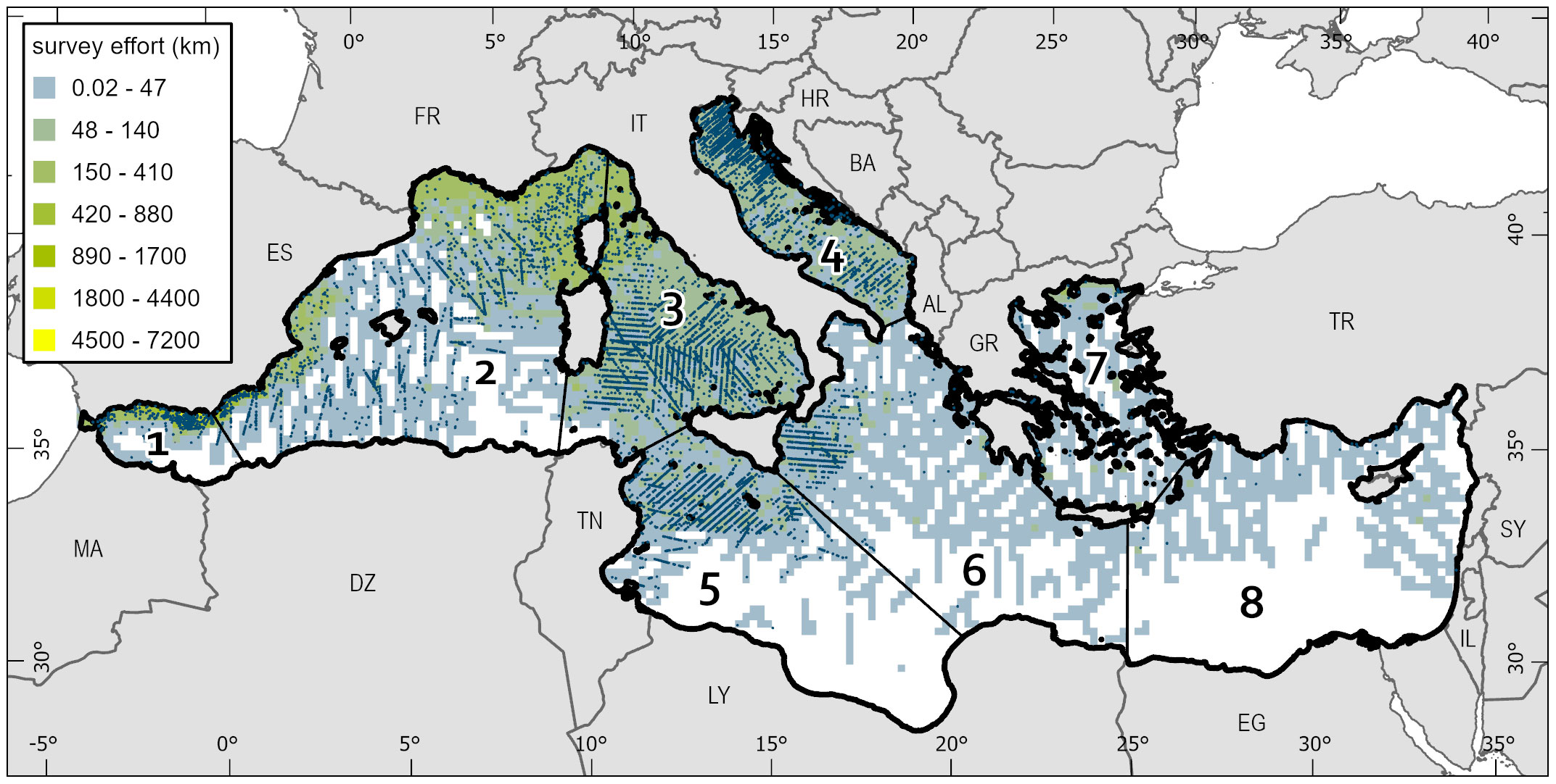
Figure 1 The study area within the Mediterranean Sea (black outline) over which abundance predictions are made. Subregions are separated by thinner black lines and are defined as 1) Alborán Sea/Strait of Gibraltar, 2) Algero-Provençal Basin, 3) Tyrrhenian Sea/eastern Ligurian Sea, 4) Adriatic Sea, 5) Strait of Sicily/Tunisian Plateau/Gulf of Sirte, 6) Ionian Sea/Central Mediterranean, 7) Aegean Sea, and 8) Levantine Sea. Survey effort (linear km of effort per 400 km² grid cell) is provided as a surface with turtle observations shown as small blue dots. 2-digit country codes for select countries are provided for reference (clockwise from top): ES, Spain; FR, France; IT, Italy; HR, Croatia; BA, Bosnia and Herzegovina; AL, Albania; GR, Greece; TR, Turkey; SY, Syria; IL, Israel; EG, Egypt; LY, Libya; TN, Tunisia; DZ, Algeria; MA, Morocco.

TABLE 1

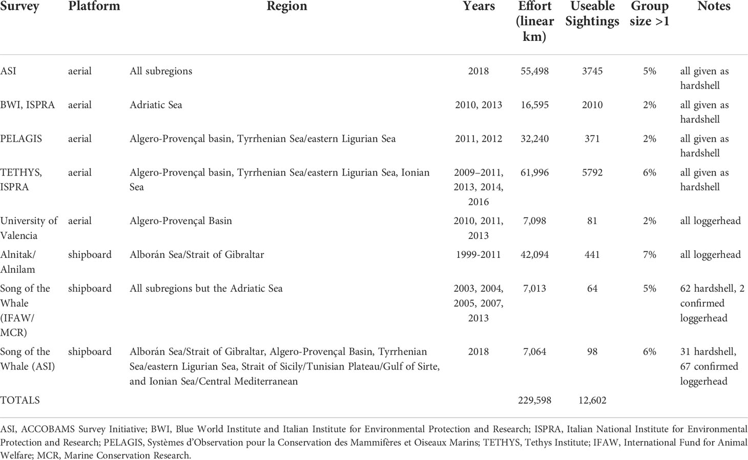
Table 1 Summary of survey effort and sightings used in the loggerhead turtle models.

All surveys but the ACCOBAMS Survey Initiative (ASI) survey were usable in a distance sampling framework, and we ensured that they contained all the requisite components to perform distance sampling – time, location, the number of animals detected (e.g. group size), and perpendicular distance to the animal(s) from the trackline (Buckland et al., 2001). The ASI survey used a strip transect sampling protocol.

Line transects were split into 5-km segments, the same resolution as the finest scale candidate environmental covariates for the spatial density models. Not all transects could be split into perfectly even 5-km segments, so an algorithm was used to split the segments as close to 5-km as possible (Mannocci et al., 2018).

All loggerhead turtle sightings, as well as unidentified hardshell turtle sightings, were used in the model (Table 1). In aerial surveys it can be difficult to discriminate loggerhead from green turtles (Chelonia mydas); hence, in some surveys, sightings were assigned to the species most likely to occur in the region (loggerhead turtles) or all recorded as unidentified. Unidentified sightings could reasonably be assumed to be mostly loggerhead turtles based on their much larger population than green turtles (Casale and Heppell, 2016). With few exceptions green turtles are limited to the Eastern Mediterranean. In the western Mediterranean, 98% of stranded turtles are loggerhead turtles (Tomás et al., 2008).

2.2 Detection function fitting

Detection functions, monotonically decreasing functions used to describe the relationship between probability of detection and distance to an observation (Buckland et al., 2001), were fit for the six surveys that used distance sampling protocols and were subsequently used to predict segment abundance.

Histograms of perpendicular distances were generated for each of the six surveys to explore the need for truncation. Buckland et al. (2001) recommends that distant sightings are truncated (‘right truncation’) to maintain a minimum probability of detection of 0.15. Left truncation, e.g. removing sightings near the trackline, is generally only used in special circumstances, such as when the trackline is not visible. This was performed for only the University of Valencia aerial surveys which used aircraft with flat windows, limiting the view of the trackline.

The ability to sight animals generally varies by survey platform and protocol. As such, it is desirable to fit separate detection functions by platform and survey if there are enough sightings to meet the recommended 60 sighting threshold for fitting robust detection functions (Buckland et al., 2001).

All surveys had more than the recommended 60 sightings, so no pooling was required between surveys or platforms. We pooled multiple years of the same survey program to be able to fit more complex detection functions, unless there was good reason not to pool, such as different altitudes between years. Most surveys had associated survey condition and sightings covariates that allowed multi-covariate distance sampling (Marques and Buckland, 2004), meaning the probability of detection varies as a function of the covariates.

All combinations of survey condition and sighting covariates were attempted for both half normal and hazard rate detection functions, the two most common forms for the detection function (Buckland et al., 2001), both with and without cosine transformations. Additional covariates tested in combination with the others included year (for surveys with multiple years), month, and observer position. Group size was not included as a covariate, as is common for marine mammals, because turtles are not gregarious creatures and rarely aggregate except for the purposes of mating. Table 1 summarizes available sightings per survey and percent of group sizes larger than one.

Detection function model selection was based on Akaike Information Criteria (AIC), which is used to assess the trade-off between goodness of fit and model simplicity. We selected the model with the lowest AIC. If more than one ‘best’ model had similar AIC (within 2) we chose between them based on goodness of fit statistics (Cramer-von Mises and Kolmogorov-Smirnoff), parsimony (degrees of freedom), and qualitative assessments of quantile-quantile (Q-Q) plots and detection plots.

The ASI aerial survey did not record perpendicular distances to sea turtles, instead opting for a strip transect approach. The survey data providers assumed all sea turtles within a 200-meter strip on either side of the plane were detected (ACCOBAMS, 2021). With a strip transect methodology, no detection function is fit and abundance per segment is calculated by dividing the number of individuals sighted by the area covered and adjusted for availability and perception bias if possible.

2.3 Correction for availability bias

No surveys obtained for this study had the requisite information to assess perception bias in-situ. We opted not to use published estimates of perception bias as they are very survey platform and condition specific.

Three datasets of loggerhead turtles deployed with satellite-linked, time depth recorders were used for calculating dive and surface intervals appropriate for making availability bias adjustments (Broderick et al., 2007; Hochscheid et al., 2007; Hochscheid et al., 2010; Hochscheid et al., 2013; Chimienti et al., 2020; Haywood et al., 2020; Hochscheid, 2020; Oceanographic Turtles Project, 2020; Society for the Protection of Turtles, 2020). These tags recorded dive and surface intervals, as well as georeferenced animal locations, allowing dives to be linked to specific locations. Availability bias is calculated as average surface interval divided by average surface interval plus average dive length.

Tagged animals from the three datasets were deployed in waters off Cyprus, Italy, and Spain respectively. Animals ranged across all regions of the Mediterranean Sea included in this study except for the Adriatic Sea and Aegean Sea. Table 2 summarizes the available data.

TABLE 2

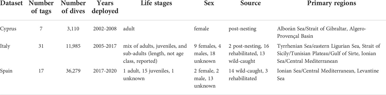
Table 2 Summary of available dive data for availability bias estimates.

The Italy and Cyprus dive datasets had similar formats with dive duration and surface intervals given in seconds along with dates and times for the start and end of the dives. Georeferenced locations, a combination of global positioning system (GPS) and Argos satellite system locations, were provided separately along with dates and times. Argos location classes 3, 2, 1, and 0 were considered valid as were all GPS locations. Dives were matched to the closest location within six hours on the assumption that remotely sensed environmental covariates would not change appreciably over the distance a turtle could swim in 6 hours. Dives that could not be georeferenced to a location within six hours were removed from the analysis.

For both datasets, tags were configured to consider a dive to have started when the turtle dove below 4 m. In good viewing conditions for aerial surveys (low turbidity, low Beaufort sea state, etc.) turtles can be seen as deep as 3 m, though the chances of detecting turtles decreases as depth increases (Fuentes et al., 2015; Barco et al., 2018). The viewable depth for turtles is likely shallower for shipboard surveys as the viewing angles preclude seeing down into the water column. Because of this decreased detection chance, we are likely overestimating the amount of time animals are available to be seen because some portion of the animals will be deeper than can be seen or will be harder to detect by observers. This would have the effect of underestimating abundance.

Tags for the Spain dataset were formatted to record depths over five-minute intervals and reported the average depth of the five-minute period. Each five-minute average depth was georeferenced to a location generated from a state-space switching model track of animal locations. These five-minute averages were then used to generate dive profiles. Surface and dive intervals were created from these dive profiles. Based on tag configuration, dives were defined to start when the turtles went below 3 m.

Short surfacing events of a few minutes or less may have been missed in the Spain dataset, as average depths were reported over five-minute intervals. This is likely not an issue for aerial surveys, which can generally be treated as instantaneous snapshots of the surface, but underestimation of availability could occur for shipboard surveys (overestimating abundance).

Surface intervals longer than four hours were removed from all three datasets. Surface times of this length could be indicative of a nesting event, basking, mating, or a failure of the saltwater switch that indicated when the turtle was below the surface. Removing these events depresses availability estimates, increasing abundance. These long surface intervals were less than one percent of all dive records.

The 51,373 remaining georeferenced dives were stratified spatially and temporally to determine if significant differences in dive behavior, and hence availability, existed. Turtles have diurnal changes in dive behavior (Hochscheid, 2014), so only daytime dives were included in this analysis, which is also when surveys would have occurred.

The temporal split was into two broad seasons–warm and cool–based on major climatic shifts in temperature and increases in neritic turtle activity. The warm season was defined as May-October and cool as November-April. Spatial stratification was into neritic versus oceanic regions, split at the 200 m isobath, where animals would presumably be feeding on different prey and exhibiting different dive behavior (Hochscheid, 2014). This also partially addresses differences in behavior between presumed larger, neritic adults and smaller, oceanic individuals.

For the long-term model, abundance for each segment was calculated using a Horvitz-Thompson-like estimator (Borchers et al., 1998). The availability bias estimate for each segment was adjusted based on platform-specific speed, height, and viewing angles, which can be found in Mannocci et al. (2018). Bubble window aerial surveys were adjusted after Carretta et al. (2000). Flat window surveys and shipboard surveys were adjusted using equations seven and four respectively from Laake et al. (1997). For the summer 2018 model, availability bias adjustments were applied after modeling, as the unadjusted model was used in the in the ACCOBAMS Survey Initiative report (ACCOBAMS, 2021) and was created using methods consistent with models for other taxa presented in that report.

2.4 Spatial modeling

2.4.1 Environmental covariates

Potential environmental covariates that could be associated with marine turtle habitat were compiled for the study area. For the long-term model, six static covariates and ten dynamic covariates (three physical and seven biological) were selected that were available at a monthly resolution and spanned the temporal range of the study.

For the summer 2018 model, covariates consistent with the other ACCOBAMS models (ACCOBAMS, 2021) were used as candidates and included 18 static covariates and 10 dynamic covariates at monthly and seasonal resolution. Latitude and longitude were included as potential covariates for the summer 2018 model but not the long-term model.

Including spatial smooths is a common practice in spatial density modeling to account for variability not captured by the available environmental covariates. It was not used in the long-term model because a spatial smooth cannot easily be extrapolated, which would necessitate using separate models for any areas of geographic extrapolation. Additionally, a spatial smooth is most influential where sightings occur, which can cause issues when survey coverage is uneven, as is the case with the long-term model.

Different sets of covariates were used for the long-term and summer 2018 models because the summer 2018 model needed to be consistent with other ACCOBAMS models and was originally produced as part of that project. Not all the covariates used in the summer 2018 model were available for the time period of the long-term model. Only contemporaneous dynamic covariates were included in both models, rather than climatological covariates, on the assumption that turtle distribution is more closely related to ephemeral conditions than long-term averages of conditions (Howell et al., 2015). Details on the covariates considered can be found in Table 3.

TABLE 3

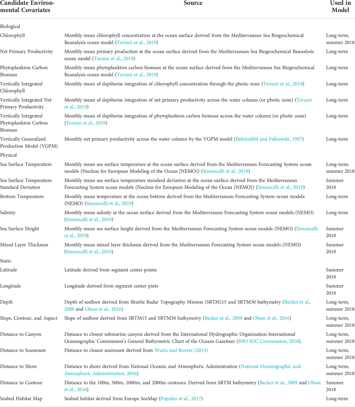
Table 3 Candidate environmental covariates for inclusion in spatial density models.

All covariates were processed to 5 x 5 km grid cells for the long-term model and 10 x 10 km grid cells for the summer 2018 model using a nearest neighbor resampling method. The center points of the processed grid cells were sampled and used for model prediction. Because some extreme values of covariates were poorly sampled by surveys, the extent of environmental extrapolation was assessed for the long term model using the R package dsmextra (Bouchet et al., 2019). The methods and results of the extrapolation analysis are presented in the Supplemental Material.

2.4.2 Density modeling

A generalized additive model (GAM) framework was used for both the long-term and summer models. The response variable, predicted abundance, was modeled with a Tweedie distribution (Foster and Bravington, 2013), which handles zero-inflated distributions well. This is useful because most segments had zero sightings and, therefore, an abundance of zero. All models were fit with the R package mgcv (Wood, 2011).

Candidate models for the long-term model were fit to all segments from survey data between 2003 and 2018. Only segments from the ACCOBAMS aerial survey were used for the summer 2018 model.

Predictions from the long-term model were made monthly, the finest temporal scale of the dynamic covariates. Cells from each monthly prediction were averaged into a single prediction covering the time span of the study period, creating a ‘densitology’ prediction of long-term abundance over the 16 years. This assumes that loggerhead abundance was relatively stable over this period, which may not be true given the apparent increasing trend in nesting females (Casale et al., 2018). Cells were treated as independent units for predictions.

A single model prediction was made for summer 2018, as well as a conventional abundance estimate using a 400-meter strip transect. For the conventional estimate, the density of the animals was estimated for each strip (searched area), dividing the number of animals detected by the searched area. The individual strip densities were averaged then extrapolated to the whole study area by multiplying the average density by the total area.

For both long-term and summer 2018 spatial density models, candidate models were fit with all possible combinations of available covariates attempted. The exception was covariates that were highly correlated. Correlation was examined using Spearman’s correlation coefficient, and if covariates had a score of 0.5 or higher, only one was retained. A review of scatter plots of covariate interactions did not indicate non-linear relationships were present.

The maximum degrees of freedom, or wiggliness, for the relationship between covariates and the response variable was allowed. Thin-plate regression splines with shrinkage were used to allow the effect of non-significant variables to ‘shrink’ away to zero (Wood, 2003). Given the large number of segments with sightings, no attempt was made to limit the number of covariates included in the model if they were significant. Model selection was accomplished by choosing the model with the lowest Restricted Maximum Likelihood (REML) score, which may be less prone to local minima than other selection criteria (Wood, 2011). We checked model goodness of fit by examining residuals, utilized degrees of freedom, and by qualitatively assessing models for unrealistic artifacts or predictions.

2.4.3 Uncertainty estimation

For both models, a parametric bootstrap approach was conducted to account for two sources of uncertainty: model parameter uncertainty and environmental variability as in Becker et al. (2014). After model fitting and selection, resampled parameter estimates from the selected model based on their associated uncertainty were drawn and new predictions were made based on the resampled parameters, also called posterior simulation (Bravington et al., 2021).

For the long-term model, 200 draws were made for each month, creating a set of 200 abundance predictions for each month that varied based on the uncertainty of the parameter space of the selected model relative to the underlying environment. Only one set of predictions was generated for the summer 2018 model as it was treated as a single time period. Coefficient of variation (CV) was calculated based on these abundance predictions, which combined the model parameter uncertainty and environmental variability.

An additional source of uncertainty was included in the overall CV calculation for the summer 2018 model. The delta method was employed to combine the CV from the parametric bootstrap and the variation among the samples used in the model (individual strip transects).

3 Results

3.1 Segments and detection functions

Some sightings were removed because they were missing detection function covariates or perpendicular distances. Any survey segments with removed sightings were eliminated from all subsequent analyses. The percentage of on effort sightings eliminated from surveys ranged from 4.7% (University of Valencia) to 0% (PELAGIS) with 0.7% of sightings removed overall.

Table 4 summarizes the selected detection function, covariates, and truncation distances for all surveys where distance sampling protocols were followed. Review of the detection function goodness of fit statistics and plots indicated good fit for most detection functions.

TABLE 4

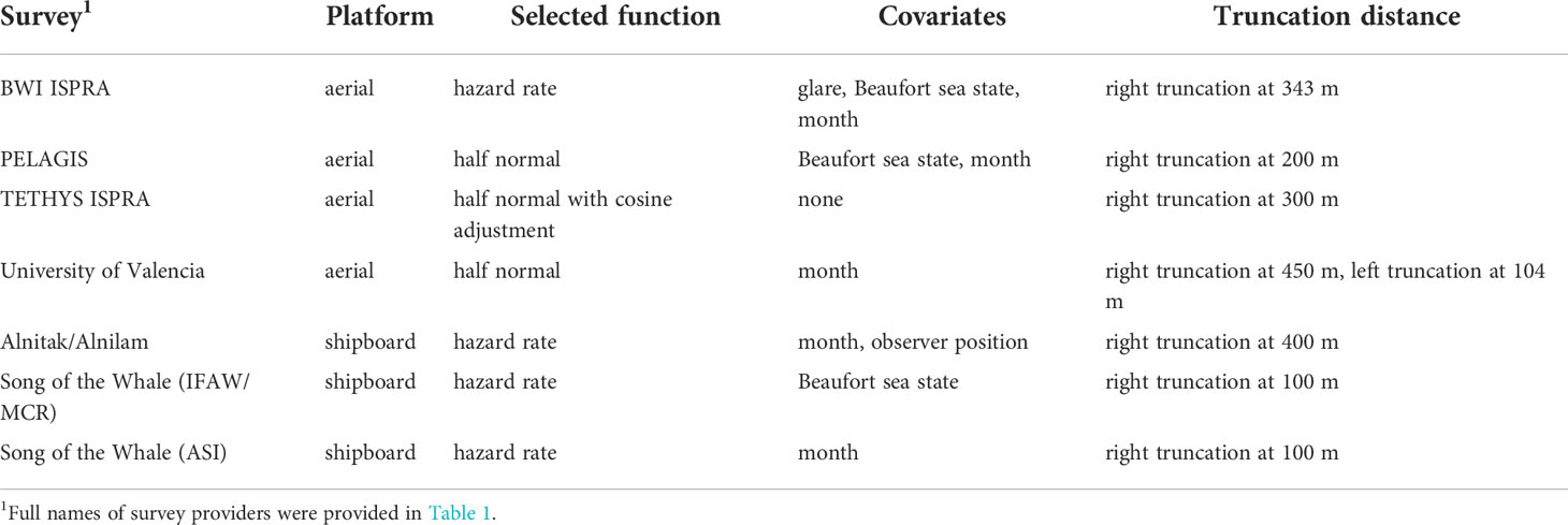
Table 4 Summary of selected detection function models for surveys with distance sampling protocols.

For the TETHYS and ISPRA aerial surveys, there was some potential heaping on the trackline (e.g. more sightings on the trackline than would be expected). There was no clear way to address this heaping. However, detection functions are generally robust to this issue (Buckland et al., 2001), and the normal model selection process was applied.

The University of Valencia surveys were flown at different heights between survey years, so separate detection functions were initially attempted for the different years. There were only 34 sightings in the 2010/2011 surveys. The Q-Q plots for models fitted to those surveys indicated poor fit and could not include any covariates with so few sightings, so instead the years were combined, and survey year was included as a potential covariate. The selected detection function was the half normal, left truncated at 104 m with month as the only covariate. The Q-Q plot was not as good as for other aerial surveys, but this was unsurprising given the relatively lower number of sightings, the need for left truncation, and the different altitude between years.

3.2 Correction for availability bias

Significant differences in dive duration and surface interval were identified by all three stratifications: day/night, depth, and warm/cool season (t-test, all p values < 0.05). Based on this finding, availability bias estimates were generated using daylight dives only, and then stratified by season and depth. This approach yielded four different availability bias adjustments based on the mean dive and surface intervals. There was high variability among the dives, and standard deviations of the intervals often exceeded the mean (Table 5). This variability is not accounted for in the CV of the final models, as at the time of analysis there was not a computationally feasible method for propagating this uncertainty. Instantaneous g(0) availability bias adjustments ranged from 0.48 for oceanic areas in the summer to 0.27 in neritic areas in the winter (Table 5).

TABLE 5

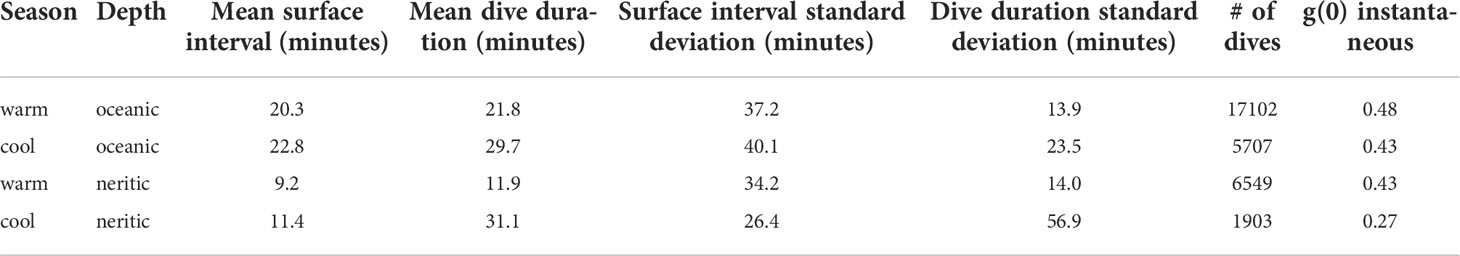
Table 5 Stratified availability bias, g(0), estimates for the Mediterranean Sea based on in-situ dive data.

3.3 Spatial models

The best long-term model retained all candidate covariates. It had the best deviance explained (34%) and lowest REML score of all candidate models. Figure 2 shows the functional relationships to covariates fit by the long-term model. Extreme values of chlorophyll a, depth, slope, and salinity were poorly sampled (see rug plots in Figure 2) and had higher associated uncertainty. For dynamic covariates, apparent preferences were for warmer temperatures, higher productivity, and lower salinity. The relationships with static covariates led to higher predicted abundance in offshore areas.

FIGURE 2

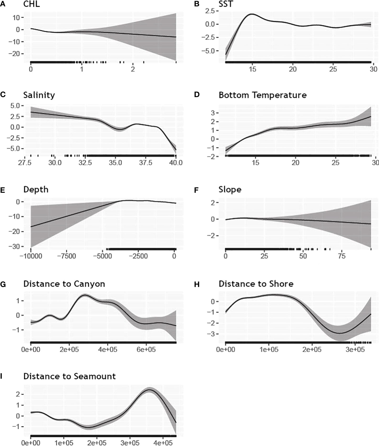
Figure 2 Functional plots of the relationships between environmental covariates and abundance for the long-term model. All plots are single covariate smooths with unlimited degrees of freedom. Uncertainty is shown by the gray shaded areas. Rug plots demarking sampled values are represented by ticks on the x-axis. Panels and abbreviations: (A) CHL – mean chlorophyll concentration at the ocean surface (mg/L), (B) SST – mean sea surface temperature (degrees Celsius), (C) Salinity– mean salinity (ppm), (D) BT – mean bottom temperature (degrees Celsius), (E) Depth – bottom depth (m), (F) Slope – bottom slope (degrees), (G) Distance to canyon (m), (H) Distance to shore (m), (I) Distance to sea mount (m).

The total predicted abundance was 1,201,845 (CV=0.22, 95% CI [838,864-1,548,280]) for the long-term model and included adjustments for availability bias. Abundance values by grid cell can be seen in Figure 3A. The overall CV estimate includes both GAM parameter uncertainty and environmental variability. The abundance in the areas of geographic extrapolation was 192,826 (Figure 3A). The extent of geographic extrapolation and the percent of the total predicted abundance that was in the areas of geographic extrapolation was approximately the same (16%).

FIGURE 3

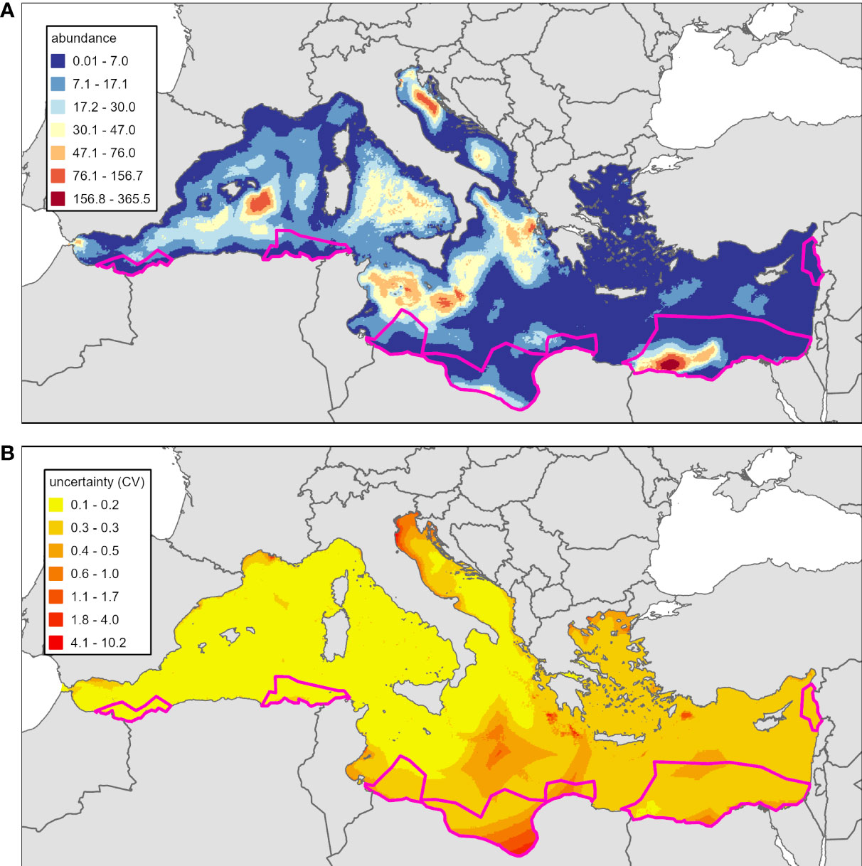
Figure 3 Long-term loggerhead turtle abundance predictions adjusted for availability bias (panel A) for the Mediterranean Sea and associated uncertainty, measured as coefficient of variation (panel B). The spatial scale of predictions for this figure is the number of animals in each 25km² grid cell. Areas highlighted in pink are areas of geographic extrapolation.

The highest predicted abundances were in the southeastern Mediterranean off the coast of Egypt, the northern Adriatic Sea, the southern Algero-Provençal Basin to the Balearic Islands, and the Tunisian Plateau. Predicted abundance was low in most coastal areas, the Aegean Sea, and the eastern Mediterranean Sea (except for the hotspot off Egypt). An assessment of inter- and intra-annual variability of monthly abundance predictions for the long-term model is presented in the Supplemental Materials.

There were high values of CV (greater than 1) located around areas of low salinity, far distances to canyons, and extremely deep areas that were poorly sampled by surveys. For example, the northern Adriatic Sea, the Libyan coast, and off the coast of Crete all had high values of CV (Figure 3B). CV was generally lower in well sampled areas.

The selected covariates for the summer 2018 model were latitude, longitude, distance to shore, distance from canyons, mean mixed layer thickness, and standard deviation of sea surface temperature. Like the long-term model, higher densities were predicted further from shore and canyons. Turtles appeared to avoid areas at extreme ranges of mean mixed layer depth and areas with high variability in temperature (Figure 4).

FIGURE 4

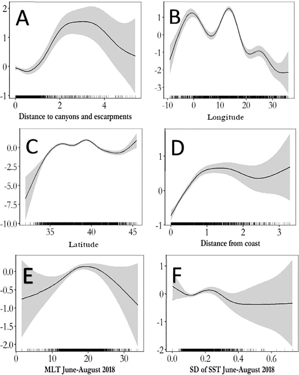
Figure 4 Functional plots of the relationships between environmental covariates and abundance for the summer 2018 model. All plots are single covariate smooths with unlimited degrees of freedom. Uncertainty is shown by the gray shaded areas. Rug plots demarking sampled values are represented by ticks on the x-axis. Panels and abbreviations: (A) Distance to canyons and escarpments (m), (B) smooth of longitude, (C) smooth of latitude, (D) distance from shore (m), (E) MLT – mean mixed-layer depth (m); (F) SD of SST – standard deviation of sea surface temperature (degrees Celsius).

The summer 2018 (uncorrected for availability bias) abundance estimate was 343,321 turtles (CV=0.03) in the whole Mediterranean except the unsurveyed southeastern region, a similar area to what was extrapolated for the long-term model. Abundance and CV values by grid cell can be seen in Figure 5. The total abundance of the spatial model was similar to the results obtained from the strip transect analysis: 329,529 individuals (CV=0.05). These results include 2,252 turtles estimated in contiguous Atlantic waters of South Portugal, to the west of the Strait of Gibraltar, where predictions were not made for the long-term model. The highest abundances were predicted in the Central and Western Mediterranean and the Adriatic Sea. The lowest abundance was predicted in the Eastern Mediterranean, approximately 20 times lower than the higher abundances predicted elsewhere.

FIGURE 5

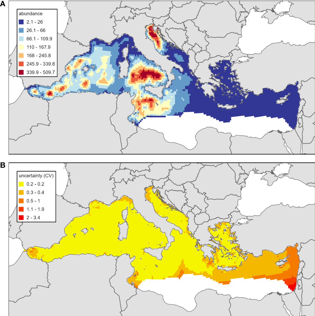
Figure 5 Summer 2018 loggerhead turtle abundance predictions unadjusted for availability bias (panel A) for the Mediterranean Sea and associated uncertainty, measured as coefficient of variation (panel B). The spatial scale of predictions for this figure is the number of animals in each 100km² grid cell. This differs from Figure 4 where the long-term model was predicted with 25km² grid cells. For the summer 2018 model, geographic extrapolation into unsurveyed areas of the southeastern Mediterranean Sea was not pursued.

Adjusting the summer 2018 model for availability bias using the same warm month and depth availability bias estimates as the long-term model, the corrected abundance estimate is 789,244 turtles. This estimate does not include any predictions for the southeastern Mediterranean. The long-term model predicts 1,009,550 (95% CI [787,449-1,231,651]) turtles in the same area (areas covered the ASI survey). Considering the CIs of the two estimates, there is some overlap between the predictions.

4 Discussion

This study presents the first estimates of loggerhead turtle distribution and abundance across the Mediterranean Sea which are not derived from demographic modeling of nesting females, and which include loggerhead turtles of Atlantic origin. Both a long-term average estimate from 2003-2018 and a summer 2018 estimate were derived from line transect survey data to inform management at basin and regional scales. Despite sources of uncertainty in the modeling process, these models represent the best estimates of the numbers and distribution of loggerhead sea turtles at basin-wide scales in the Mediterranean Sea.

The similarity in abundance estimates and spatial pattern between the long-term model and summer 2018 estimates may indicate that summer distribution of loggerhead turtles may be driving the patterns predicted by the long-term model. This is unsurprising given that most of the survey effort used in the long-term model occurred in warm months.

For the long-term model, seasonal models were initially attempted, as there is evidence that animals migrate seasonally from the eastern to western basins and from the eastern basin to the Adriatic Sea (summarized in Mazor et al., 2016; Casale et al., 2018). Cool season models performed poorly and did not seem realistic, so seasonal models were not presented. This was likely driven by lower survey coverage in the cool season and less uniform spatial coverage.

Low abundance in the eastern Mediterranean was predicted by both the long term and summer models. Despite the eastern Mediterranean being the largest concentration of nesting on the region, nesting females account for a very small percentage of the total population and juveniles range widely in their oceanic stage.

While most of the spatial abundance predictions appear reasonable based on the sightings data, the hotspot off Egypt in the long-term model (area of geographic extrapolation, Figure 5) should be treated with caution given that there is no survey coverage in that area. The hotspot has the highest predicted abundance values in the model.

Rabia and Attum (2015) found evidence of loggerhead turtles stranding on the Egyptian coast, and Rabia and Attum (2020) observed sea turtles foraging in Lake Bardawil in Egypt. Additionally, the continental shelf off Egypt’s Nile Delta hosts foraging sites for loggerhead turtles nesting in Cyprus and the southern coast of the eastern Mediterranean is a migratory corridor for turtles traveling from Cyprus to the east coast of Tunisia (Snape et al., 2016; Haywood et al., 2020). Despite this evidence that turtles are present in the waters off Egypt and migrate through the area, this hotspot should be treated with caution until line transect data covering this area can be included in models.

With a few exceptions, the models predicted lower abundance in coastal and neritic areas, where large juveniles and adult turtles are known to forage, particularly in the eastern Mediterranean. These neritic foraging areas have been confirmed by multiple lines of investigation (Casale et al., 2018). Exceptions to low predictions in coastal areas were the Tunisian Plateau, the northern Adriatic Sea, and the hotspot off Egypt. It may be that not all neritic areas host the appropriate prey base for neritic turtles. More research into prey distribution would be needed to confirm this thesis.

The models can best be considered models of oceanic loggerhead turtles, which represent most loggerheads in the Mediterranean Sea (Casale and Heppell, 2016). Some adult loggerhead turtles may be found in oceanic habitats, either while migrating, or if they have never recruited to neritic areas (Luschi et al., 2018). Mediterranean loggerhead nesting females are the smallest in the world (Tiwari and Bjorndal, 2000) and small adults in other regions have been shown to sometimes remain oceanic foragers (Hawkes et al., 2006).

When considering these models for management purposes, some important neritic foraging areas for older turtles may be overlooked, specifically, large individuals of high reproductive value, which may be particularly subject to high bycatch mortality in coastal fisheries (Casale, 2011; Lucchetti et al., 2021). Coupling these models with other data sources such as satellite telemetry and stable isotope analyses will be critical for holistic management of the loggerhead turtle population in the Mediterranean Sea.

Environmental covariates were poorly sampled close to shore, and there were grid cells where predictions were not made within 5-10 km of shore. A decision was made to not extrapolate the models into these unsampled grid cells as they were also poorly sampled by surveys. This is a source of underestimation of abundance in the model. The missing cells represent 0.05 percent of the area of the Mediterranean Sea. If estimates are needed close to shore for management purposes, extrapolating values from nearby cells is a possible solution. However, these are broad scale models intended for basin-wide and regional abundance estimation and conservation action. We caution against relying on estimates from individual cells for fine scale management.

Satellite telemetry data featured in the State of the World’s Sea Turtle Report (SWOT Team, 2019) showed loggerhead turtles to be distributed almost throughout the entire Mediterranean Sea, though fewer locations were recorded in the north-central Mediterranean and eastern Mediterranean. Higher densities of satellite telemetry locations were found in the Alboran Sea, Tunisian Plateau, Adriatic Sea, and Tyrrhenian Sea. These areas of relatively higher and lower density of satellite telemetry locations correlate well with the models’ predicted distribution, though caution must be taken when comparing spatial density models to density of satellite telemetry locations. There are significant biases associated with satellite telemetry, such as deployment bias, individual behavior, and the age classes tagged. Despite these biases, the SWOT Team (2019) report featured hundreds of tagged animals, and the general concurrence of our model and the tag data is good.

The models presented in this study also concur well with demographic population estimates. Casale and Heppell (2016) presented a demographic model of the Mediterranean loggerhead turtle population based on the number of adult females, reproductive output, and assumptions about age of sexual maturity. That study represented a completely independent population estimate from the spatial density models. Casale and Heppell (2016) made three estimates of loggerhead turtle population, assuming age of sexual maturity at 21, 25, and 34 years old. The estimates were 1,197,087 (CI 805,658-1,732,765), 1,521,107 (CI 1,034,839-2,178,790), and 2,364,843 (CI 1,611,085-3,376,104) respectively. The population estimate from the long-term model of 1,201,845 (95% CI [838,864-1,548,280]) was statistically similar (e.g. estimates overlapped when considering uncertainty) to the 21- and 25-year scenarios but not the 34-year scenario. The summer 2018 model was only statistically similar to the 21-year scenario. This may provide support to the lower age of maturity scenarios which aligns with the small size of Mediterranean adult loggerhead females. However, it is likely the spatial density models are underestimating both abundance and uncertainty (see discussion below). The concurrence of these independence estimates lends credence to both estimates as being valid, though caution is merited in comparing the two as the demographic estimates do not include turtles of Atlantic origin and may also be underestimates of total loggerhead population.

It is important to acknowledge that both models in this study and the demographic population estimates are single point estimates of population. More research is needed to determine if changes in population abundance are occurring, such as repeated, stratified abundance estimates covering the same area. This study, which combines multiple surveys over different time periods, geographic areas, and abundance varying with environmental covariates, is not the best study design for detecting trends. There is some evidence of colonization of the eastern basin by individuals from other nesting stocks and nesting within the Mediterranean may be increasing (Casale and Tucker, 2017; Carreras et al., 2018). Abundance estimates based on repeated stratified estimates could provide an additional line of evidence for population growth in the region.

As in most spatial density models, there are potential sources of bias in our estimates that merit discussion, even though the estimate is statistically similar to independent demographic population estimates. Possible sources of underestimation include the following: not accounting for perception bias, overestimating the amount of time animals are at the surface based on the depth at which dives were assumed to be started (3-4 m for dive data), missing cells close to shore due to missing environmental covariates, and not detecting small animals.

Aerial surveyors have indicated an ability to detect animals as small as 40 cm (Barco et al., 2018); however, animals of that size may be several years old already. Given the age structure of sea turtle populations, those missed animals represent a large fraction of the total population (Mazaris et al., 2005; Casale and Heppell, 2016).

Possible sources of overestimation of population include the following: including sightings reported as hardshell turtles that may actually be green turtles and including the dive data from Spain that may be missing some surfacing events. There were too few confirmed sightings of green turtles (less than 10) to attempt to use machine learning or other discrimination techniques to assign unidentified turtles to be either green or loggerhead turtles.

Green turtles may comprise as much as 50% of sea turtles in the Eastern Mediterranean if maximum population estimates for green turtles and minimum population estimates for loggerhead turtles are assumed (Casale and Heppell, 2016), though this extreme case seems unlikely. Mitigating this, Mediterranean green turtles recruit to near-shore neritic habitats at a curved carapace length of 27-40 cm (Türkozan et al., 2013; Bektaş, 2018) which is the close to the minimum CCL at which sea turtles are detectable by aerial survey methods (Barco et al., 2018). Since the surveys used to develop the spatial density models only partially cover near-shore habitats where larger green turtles recruit, and smaller oceanic green turtles are not likely to be detected, we expect the false positive identification of green turtles as loggerhead turtles to have low or negligible, though unavoidable, net contribution to estimates of distribution and abundance of loggerhead turtles. Green turtles can be found in the Levantine Basin, the Strait of Sicily/Tunisian Plateau/Gulf of Sirte, the Ionian Sea/Central Mediterranean, and the Aegean Sea subregions.

Overall, we posit that we are generally underestimating abundance because missing small turtles is likely the largest effect, given the size of those age classes relative to the total population. Additionally, there are more sources of possible underestimation than overestimation.

Some sources of uncertainty were not accounted for in either model, including measurement error in distances to sightings, variability in dive behavior, and uncertainty and daily variation in covariate values. The long-term model did not account for the variability from detection functions. This was not applicable to the strip transect approach used in the summer 2018 model. Because we are underestimating variability in our predictions, the reported CVs only account for a portion of the variability in the model. Actual variability may be much higher, and this should be taken into consideration when making management decisions based on these data.

These spatial density models can be used by regional managers to estimate impacts to loggerhead turtles from military training and testing exercises, offshore renewable energy projects, and fisheries interactions at broad spatial scales, with appropriate understanding of the limitations of these models. They can also serve as an important input into regional marine spatial planning efforts that require spatially explicit estimates of distribution and abundance. The results also support efforts to understand the distribution of the combined populations of Mediterranean and Atlantic loggerhead turtles in the Mediterranean Sea.

4.1 Future directions

While the models presented here represent an excellent first attempt at a basin-wide spatial density model for the Mediterranean Sea, there are improvements that can be made.

There are additional survey data that could be added to the survey dataset, mostly from the University of Valencia as well as from new winter shipboard surveys in the eastern Mediterranean associated with the ASI that was not available when this study was undertaken. The eastern Mediterranean is data poor already, and cool season surveys are a critical data gap. Inclusion of the new ASI survey and any future cool season surveys may allow for seasonal models to be fit. Drone surveys, though often at smaller spatial scales than the broad scales surveys used here, may also prove useful in surveying neritic foraging areas and can be used in a spatial density modeling framework the same way other strip survey transects can.

To address the issue of missing neritic foraging areas for larger turtles, two possible solutions are: 1) fit separate models to neritic and oceanic areas, or 2) fit a single model to all the data but use a hierarchical GAM framework with habitat included as a factor (Pedersen et al., 2019). Additional research into adult turtle behavior and distribution, particularly in the western basin, could help refine this future work. The same hierarchical approach could be applied to the various sub regions of the Mediterranean to see if environmental relationships are similar across the regions.

While the stratified availability bias estimates used here better reflect changing dive behavior over time and space than a single estimate, a more complex treatment may be possible given the amount of available data. Modeling availability spatially in response to environmental covariates would allow for smooth relationships over time and space, unlike the current stratified estimates that have distinct boundaries spatially and temporally. Lastly, including more sources of uncertainty in the overall estimate of CV (such as dive variability) would give users of the models a better understanding of the limitations of the models. Recent work has shown this is possible but was outside the scope of this project (Bravington et al., 2021).

Data availability statement

Some of the data used in this study are currently unpublished and are not available publicly. Persons interested in acquiring the data should contact the survey organizations directly. The long-term abundance model and associated uncertainty are available at https://seamap.env.duke.edu/models/NUWC/Med/.

Ethics statement

This study used observations of animals previously conducted under other research efforts.

Author contributions

AD and AC were responsible for the concept of the paper; AD, AC, JR, and LS were responsible for data processing and analysis; AD, AC, and LS, were responsible for writing; SP, AM, CF, DH, GL, HP, JAR, OB, JT, and VR provided the line transect survey data used; AB, BG, DM, JH, RSa, RSn, and SH provided the dive data used for the availability bias analysis as well as information on sea turtle ecology in the Mediterranean.

Acknowledgments

We would like to thank all the organizations that contributed line transect surveys and dive data to this project: Blue World Institute, The University of Valencia, Tethys Institute, ISPRA, IFAW, The University of Exeter, Society for the Protection of Turtles, ACCOBAMS, PELAGIS, Alnitak, Stazione Zoologica Anton Dorne. These organizations all had their own sources of internal and external funding for their work and we are grateful to those funders for supporting the baseline research upon which this study is built.

Conflict of interest

Author AD is employed by McLaughlin Research Corporation and CheloniData LLC.

The remaining authors declare that the research was conducted in the absence of any commercial or financial relationships that could be construed as a potential conflict of interest.

Publisher’s note

All claims expressed in this article are solely those of the authors and do not necessarily represent those of their affiliated organizations, or those of the publisher, the editors and the reviewers. Any product that may be evaluated in this article, or claim that may be made by its manufacturer, is not guaranteed or endorsed by the publisher.

Supplementary material

The Supplementary Material for this article can be found online at: https://www.frontiersin.org/articles/10.3389/fmars.2022.930412/full#supplementary-material

References

ACCOBAMS (2021). Estimates of abundance and distribution of cetaceans, marine mega-fauna and marine litter in the Mediterranean Sea from 2018-2019 surveys. Eds. Panigada S., Boisseau O., Canadas A., Lambert C., Laran S., McLanaghan R., Moscrop A. (Monaco: ACCOBAMS - ACCOBAMS Survey Initiative Project), 177.

Google Scholar

Barco S. G., Burt M. L., DiGiovanni R. A. Jr, Swingle W. M., Williard A. S. (2018). Loggerhead turtle caretta caretta density and abundance in Chesapeake bay and the temperate ocean waters of the southern portion of the mid-Atlantic bight. Endang. Species Res. 37, 269–287. doi: 10.3354/esr00917

CrossRef Full Text | Google Scholar

Becker E. A., Forney K. A., Foley D. G., Smith R. C., Moore T. J., Barlow J. (2014). Predicting seasonal density patterns of California cetaceans based on habitat models. Endang. Species Res. 23, 1–22. doi: 10.3354/esr00548

CrossRef Full Text | Google Scholar

Becker J. J., Sandwell D. T., Smith W. H. F., Braud J., Binder B., Depner J., et al. (2009). Global bathymetry and elevation data at 30 arc seconds resolution: SRTM30_PLUS. Mar. Geod. 32 (4), 355–371. doi: 10.1080/01490410903297766

CrossRef Full Text | Google Scholar

Behrenfeld M. J., Falkowski P. G. (1997). Photosynthetic rates derived from satellite-based chlorophyll concentration. Limnology and Oceanography 42. doi: 10.4319/lo.1997.42.1.0001.

CrossRef Full Text | Google Scholar

Bektaş S. (2018). Sixteen year (2002-2017) record of Sea turtle strandings on samandağ beach, the Eastern Mediterranean coast of Turkey. Zoological Stud. 75. doi: 10.6620/ZS.2018.57-53

CrossRef Full Text | Google Scholar

Benson S. R., Forney K. A., Harvery J. T., Caretta J. (2007). Abundance, distribution, and habitat of leatherback turtles off California 1990-2003. Fish. Bull. 105, 337–347.

Google Scholar

Bentivegna F., Hochscheid S., Minucci C. (2003). Seasonal variability in voluntary dive duration of the Mediterranean loggerhead turtle, caretta caretta. Scientia Marina 67 (3), 371–375. doi: 10.3989/scimar.2003.67n3371

CrossRef Full Text | Google Scholar

Borchers D., Buckland S., Goedhart P., Clarke E., Hedley S. (1998). Horvitz-Thompson estimators for double-platform line transect surveys. Biometrics 54 (4), 1221–1237. doi: 10.2307/2533652

CrossRef Full Text | Google Scholar

Bouchet P., Miller D. J., Roberts J. J., Mannocci L., Harris C. M., Thomas L. (2019). From here and now to there and then: Practical recommendations for extrapolating cetacean density surface models to novel conditions (Centre for Research into Ecological & Environmental Modelling (CREEM), (St. Andrews, Scotland, United Kingdom: University of St Andrews, Scotland, United Kingdom), 59. CREEM Technical Report 2019-01.

Google Scholar

Bravington M. V., Miller D. L., Hedley S. L. (2021). Variance propagation for density surface models. JABES 26, 306–323. doi: 10.1007/s13253-021-00438-2

CrossRef Full Text | Google Scholar

Broderick A. C., Coyne M. S., Fuller W. J., Glen F., Godley B. J. (2007). Fidelity and over-wintering of sea turtles. Proc. R. Soc B 274, 1533–1538. doi: 10.1098/rspb.2007.0211

CrossRef Full Text | Google Scholar

Buckland S. T., Anderson D. R., Burnham K. P., Laake J. L., Borchers D. L., Thomas L. (2001). Introduction to distance sampling. (New York: Oxford University Press).

Google Scholar

Cañadas A., Aguilar de Soto N., Aissi. M., Arcangeli A., Azzolin M., B-Nagy A., et al. (2018). The challenge of habitat modelling for threatened low density species using heterogeneous data: The case of cuvier’s beaked whales in the Mediterranean. Ecol. Indic. 85, 128–136. doi: 10.1016/j.ecolind.2017.10.021

CrossRef Full Text | Google Scholar

Cardona L., Hays G. C. (2018). Ocean currents, individual movements and genetic structuring of populations. Mar. Biol. 165, 10. doi: 10.1007/s00227-017-3262-2

CrossRef Full Text | Google Scholar

Carreras C., Pascual M., Cardona L., Marco A., Bellido J. J., Castillo J. J., et al. (2011). Living together but remaining apart: Atlantic and Mediterranean loggerhead sea turtles (Caretta caretta) in shared feeding grounds. J. Hered. 102, 666–677. doi: 10.1093/jhered/esr089

PubMed Abstract | CrossRef Full Text | Google Scholar

Carreras C., Pascual M., Tomás J., Marco A., Hochscheid S., Castillo J. J., et al. (2018). Sporadic nesting reveals long distance colonisation in the philopatric loggerhead sea turtle (Caretta caretta). Sci. Rep. 8, 1435. doi: 10.1038/s41598-018-19887-w

PubMed Abstract | CrossRef Full Text | Google Scholar

Carreras C., Pont S., Maffucci F., Pascual M., Barceló A., Bentivegna F., et al. (2006). Genetic structuring of immature loggerhead sea turtles (Caretta caretta) in the Mediterranean Sea reflects water circulation patterns. Mar. Biol. 149, 1269–1279. doi: 10.1007/s00227-006-0282-8

CrossRef Full Text | Google Scholar

Carretta J. V., Lowry M. S., Stinchcomb C., Lynn M. S., Cosgrove R. E. (2000). Distribution and abundance of marine mammals at San clemente island and surrounding offshore waters: Results from aerial and ground surveys in 1998 and 1999 (La Jolla, California: National Marine Fisheries Service, Southwest Fisheries Science Center). Available at: https://repository.library.noaa.gov/view/noaa/3183. ADMINISTRATIVE REPORT LJ-00-02.

Google Scholar

Casale P. (2011). Sea Turtle by-catch in the Mediterranean. Fish Fisheries. 12, 299–316. doi: 10.1111/j.1467-2979.2010.00394.x

CrossRef Full Text | Google Scholar

Casale P., Broderick A. C., Camiñas J. A., Cardona L., Carrereas C., Demetropoulos A., et al. (2018). Mediterranean Sea turtles: current knowledge and priorities for conservation and research. Endang. Species Res. 36, 229–267. doi: 10.3354/esr00901

CrossRef Full Text | Google Scholar

Casale P., Heppell S. S. (2016). How much sea turtle bycatch is too much? a stationary age distribution model for simulating population abundance and potential biological removal in the Mediterranean. Endang. Species Res. 29, 239–254. doi: 10.3354/esr00714

CrossRef Full Text | Google Scholar

Casale P., Mariani P. (2014). The first ‘lost year’ of Mediterranean sea turtles: dispersal patterns indicate subregional management units for conservation. Mar. Ecol. Prog. Ser. 498, 263–274. doi: 10.3354/meps10640

CrossRef Full Text | Google Scholar

Casale P., Tucker A. D. (2017). “Caretta caretta (amended version of 2015 assessment),” in The IUCN red list of threatened species 2017. (Cambridge, United Kingdom: International Union for Conservation of Nature and Natural Resources). doi: 10.2305/IUCN.UK.2017-2.RLTS.T3897A119333622.en

CrossRef Full Text | Google Scholar

Chimienti M., Blasi M. F., Hochscheid S. (2020). Movement patterns of large juvenile loggerhead turtles in the Mediterranean Sea: ontogenetic space use in a small ocean basin. Ecol. Evol. 10, 6978–6992. doi: 10.1002/ece3.6370

PubMed Abstract | CrossRef Full Text | Google Scholar

Clusa M., Carreras C., Pascual M., Gaughran S. J., Piovano S., Giacoma C., et al. (2014). Fine-scale distribution of juvenile Atlantic and Mediterranean loggerhead turtles (Caretta caretta) in the Mediterranean Sea. Mar. Biol. 161, 509–519. doi: 10.1007/s00227-013-2353-y

CrossRef Full Text | Google Scholar

Eckert S. A., Moore J. E., Dunn D. C., van Buiten R. S., Eckert K. L., Halpin P. N. (2008). Modeling loggerhead turtle movement in the Mediterranean: importance of body size and oceanography. Ecol. Appl. 18, 290–308. doi: 10.1890/06-2107.1

PubMed Abstract | CrossRef Full Text | Google Scholar

Eguchi T., McClatchie S., Wilson C., Benson S. R., LeRoux R. A., Seminoff J. A. (2018). Loggerhead turtles in the California current: Abundance, distribution, and anomalous warming of the north pacific. Front. Mar. Sci. 6. doi: 10.3389/fmars.2018.00452

CrossRef Full Text | Google Scholar

Forney K. A., Barlow J., Carretta. J. V. (1995). The abundance of cetaceans in California waters. part II: Aerial surveys in winter and spring of 1991 and 1992. Fish Bull. 93, 15–26.

Google Scholar

Fortuna C. M., Cañadas A., Holcer D., Brecciaroli B., Donovan G. P., Lazar B., et al. (2018). The coherence of the European union marine natura 2000 network for wide-ranging charismatic species: A Mediterranean case study. Front. Mar. Sci. 5. doi: 10.3389/fmars.2018.00356

CrossRef Full Text | Google Scholar

Foster S. D., Bravington M. V. (2013). A poisson–gamma model for analysis of ecological non-negative continuous data. Environ. Ecol. Stat. 20, 533–552. doi: 10.1007/s10651-012-0233-0

CrossRef Full Text | Google Scholar

Fuentes M. M. P. B., Bell I., Hagihara R., Hamann M., Hazel J., Huth A., et al. (2015). Improving in-water estimates of marine turtle abundance by adjusting aerial survey counts for perception and availability biases. J. Exp. Mar. Biol. Ecol. 471, 77–83. doi: 10.1016/j.jembe.2015.05.003

CrossRef Full Text | Google Scholar

Gómez de Segura A., Tomás J., Pedraza S. N., Crespo E. A., Raga J. A. (2003). Preliminary patterns of distribution and abundance of loggerhead sea turtles, caretta caretta, around columbretes islands marine reserve, Spanish Mediterranean. Mar. Biol. 143, 817–823. doi: 10.1007/s00227-003-1125-5

CrossRef Full Text | Google Scholar

Gómez de Segura A., Tomás J., Pedraza S. N., Crespo E. A., Raga J. A. (2006). Abundance and distribution of the endangered loggerhead turtle in Spanish Mediterranean waters and the conservation implications. Anim. Conserv. 9, 199–206. doi: 10.1111/j.1469-1795.2005.00014.x

CrossRef Full Text | Google Scholar

Hammond P. S., Lacey C., Gilles A., Viquerat S., Börjesson P., Herr H., et al. (2021) Estimates of cetacean abundance in European Atlantic waters in summer 2016 from the SCANS-III aerial and shipboard surveys. Available at: https://scans3.wp.st-andrews.ac.uk/files/2021/06/SCANS-III_design-based_estimates_final_report_revised_June_2021.pdf (Accessed 4 March 2022). Report.

Google Scholar

Hawkes L. A., Broderick A. C., Coyne M. S., Godfrey M. H., Lopez-Jurado L. F., Lopez-Suarez P., et al. (2006). Phenotypically linked dichotomy in Sea turtle foraging requires multiple conservation approaches. Curr. Bio 16 (10), 990–995. doi: 10.1016/j.cub.2006.03.063

CrossRef Full Text | Google Scholar

Haywood J. C., Fuller W. J., Godley B. J., Margaritoulis D., Shutler J. D., Snape R., et al. (2020). Spatial ecology of loggerhead turtles: Insights from stable isotope markers and satellite telemetry. Diversity Distributions 26 (3), 368–381. doi: 10.1111/ddi.13023

CrossRef Full Text | Google Scholar

Hochscheid S. (2014). Why we mind sea turtles’ underwater business: A review on the study of diving behavior. J. Exp. Mar. Biol. Ecol. 450, 118–136. doi: 10.1016/j.jembe.2013.10.016

CrossRef Full Text | Google Scholar

Hochscheid S. (2020). Data from the movebank data repository. Accessed 19 Sept 2019. doi: 10.5441/001/1.1f1h87r8

CrossRef Full Text | Google Scholar

Hochscheid S., Bentivegna F., Bradai M. N., Hays G. C. (2007). Overwintering behaviour in sea turtles: dormancy is optional. Mar. Ecol. Prog. Ser. 340, 287–298. doi: 10.3354/meps340287

CrossRef Full Text | Google Scholar

Hochscheid S., Bentivegna F., Hamza A., Hays G. C. (2010). When surfacers do not dive: multiple significance of extended surface times in marine turtles. J. Exp. Biol. 213, 1328–1337. doi: 10.1242/jeb.037184

PubMed Abstract | CrossRef Full Text | Google Scholar

Hochscheid S., Travaglini A., Maffucci F., Hays G. C., Bentivegna F. (2013). Since turtles cannot talk: what beak movement sensors can tell us about the feeding ecology of neritic loggerhead turtles, caretta caretta. Mar. Ecol. 34 (3), 321–333. doi: 10.1111/maec.12018

CrossRef Full Text | Google Scholar

Howell E. A., Hoover A., Benson S. R., Bailey H., Polovina J. J., Seminoff J. A., et al. (2015). Enhancing the TurtleWatch product for leatherback sea turtles, a dynamic habitat model for ecosystem-based management. Fish. Oceanogr. 24, 57–68. doi: 10.1111/fog.12092

CrossRef Full Text | Google Scholar

IHO-IOC Commission. (2018). The IHO-IOC GEBCO cook book 103 Vol. 63 (France), 429. Monaco: International Hydrographic Organization, Intergovernmental Oceanographic Commission.

Google Scholar

Laake J., Calambokidis J., Osmek S., Rugh D. (1997). Probability of detecting harbor porpoise from aerial surveys: estimating g(0). J. Wild. Manage. 61 (1), 63–75. doi: 10.2307/3802415

CrossRef Full Text | Google Scholar

Laurent L., Casale P., Bradai M. N., Godley B. J., Gerosa G., Broderick A. C., et al. (1998). Molecular resolution of marine turtle stock composition in fishery bycatch: a case study in the Mediterranean. Mol. Ecol. 7, 1529–1542. doi: 10.1046/j.1365-294x.1998.00471.x

PubMed Abstract | CrossRef Full Text | Google Scholar

Lauriano G., Panigada S., Casale P., Pierantonio N., Donovan G. P. (2011). Aerial survey abundance estimates of the loggerhead sea turtle caretta caretta in the pelagos sanctuary, northwestern Mediterranean Sea. Mar. Ecol. Prog. Ser. 437, 291–302. doi: 10.3354/meps09261

CrossRef Full Text | Google Scholar

Loisier A., Savelli M. P., Arnal V., Claro F., Gambaiani D., Sénégas J. B., et al. (2021). Genetic composition, origin and conservation of loggerhead sea turtles (Caretta caretta) frequenting the French Mediterranean coasts. Mar. Biol. 168, 52. doi: 10.1007/s00227-021-03855-6

CrossRef Full Text | Google Scholar

Lucchetti A. (2021). “Sea Turtles,” in Incidental catch of vulnerable species in Mediterranean and black Sea fisheries – a review. Eds. Carpentieri P., Nastasi A., Sessa M., Srour A (Rome: FAO). Studies and Reviews No. 101General Fisheries Commission for the Mediterranean.

Google Scholar

Luschi P., Mencacci R., Cerritelli G., Papetti L., Hochscheid S. (2018). Large-Scale movements in the oceanic environment identify important foraging areas for loggerheads in central Mediterranean Sea. Mar. Biol. 165 (1), 4. doi: 10.1007/s00227-017-3255-1

CrossRef Full Text | Google Scholar

Maffucci F., Corrado R., Palatella L., Borra M., Marullo S., Hochscheid S., et al. (2016). Seasonal heterogeneity of ocean warming: a mortality sink for ectotherm colonizers. Sci. Rep. 6, 23983. doi: 10.1038/srep23983

PubMed Abstract | CrossRef Full Text | Google Scholar

Mannocci L., Roberts J. J., Halpin P. N. (2018). Development of exploratory marine species density models in the Mediterranean Sea (Durham, North Carolina: Duke University Marine Geospatial Ecology Lab). Available at: https://seamap.env.duke.edu/models/Duke/Med/. Final Report. Report prepared for Naval Facilities Engineering Command, Atlantic under Contract No. N62470-15-D-8006, Task Order TO37.

Google Scholar

Marques F. F. C., Buckland S. T. (2004). “Covariate models for the detection function,” in Advanced distance sampling. Eds. Buckland S. T., Anderson D. R., Burnham K. P., Laake J. L., Borchers D. L., Thomas L. (Oxford, United Kingdom: Oxford University Press), 31–47.

Google Scholar

Mazaris A. D., Fiksen Ø., Matsinos Y. G. (2005). Using an Individual-Based Model for Assessment of Sea Turtle Population Viability. Pop Eco 47 (2005), 179–191. doi: 10.1007/s10144-005-0220-5

CrossRef Full Text | Google Scholar

Mazor T., Beger M., McGowan J., Possingham H. P., Kark S. (2016). The value of migration information for conservation prioritization of sea turtles in the Mediterranean. Glob. Ecol. Biogeogr. 25, 540–552. doi: 10.1111/geb.12434

CrossRef Full Text | Google Scholar

Miller D. L., Burt M. L., Rexstad E. A., Thomas L. (2013). Spatial models for distance sampling data: recent developments and future directions. Methods Ecol. Evol. 4, 1001–1010. doi: 10.1111/2041-210X.12105

CrossRef Full Text | Google Scholar

Mrosovsky N. (1980). Thermal biology of Sea turtles. Am.Zool. 20 (3), 531–547. doi: 10.1093/icb/20.3.531

CrossRef Full Text | Google Scholar

National Oceanographic and Atmospheric Administration. (2016). Global self-consistent hierarchical high-resolution geography ver. 2.3.5 (Honolulu, Hawaii, USA: NOAA).

Google Scholar

Oceanographic Turtles Project. (2020). Available at: www.socib.es/tortugas (Accessed May 2020).

Google Scholar

Olson C. J., Becker J. J., Sandwell D. T. (2016). SRTM15_PLUS: Data fusion of shuttle radar topography mission (SRTM) land topography with measured and estimated seafloor topography. NCEI accession 0150537. (Silver Spring, Maryland, USA: National centers for Environmental Information).

Google Scholar

Pastor F., Valiente J. A., Khodayar S. (2020). A warming Mediterranean: 38 years of increasing Sea surface temperature. Remote Sens. 12 (17), 2687. doi: 10.3390/rs12172687

CrossRef Full Text | Google Scholar

Pedersen E. J., Miller D. L., Simpson G. L., Ross N. (2019). Hierarchical generalized additive models in ecology: an introduction with mgcv. PeerJ. 7, e6876. doi: 10.7717/peerj.6876

PubMed Abstract | CrossRef Full Text | Google Scholar

Pollock K. H., Marsh H. D., Lawler I. R., Alldredge M. W. (2006). Estimating animal abundance in heterogeneous environments: An application to aerial surveys for dugongs. J. Wildl. Manage. 70, 255–262. doi: 10.2193/0022-541X(2006)70[255:EAAIHE]2.0.CO;2

CrossRef Full Text | Google Scholar

Populus J., Vasquez M., Albrecht J., Manca E., Agnesi S., Al Hamdani Z., et al. (2017). Data from: A European broad-scale seabed habitat map. EUSeaMap. doi: 10.13155/49975

CrossRef Full Text | Google Scholar

Rabia B., Attum O. (2015). Distribution and status of sea turtle nesting and mortality along the north Sinai coast, Egypt (Reptilia: Cheloniidae). Zool. Middle East 61 (1), 26–31. doi: 10.1080/09397140.2014.994313

CrossRef Full Text | Google Scholar

Rabia B., Attum O. (2020). Sea Turtles in lake bardawil, Egypt - size distribution and population structure. Herpetol. Bull. 151, 32–36. doi: 10.33256/hb151.32-36

CrossRef Full Text | Google Scholar

Revelles M., Camiñas J. A., Cardona L., Parga M., Tomas J., Aguilar A., et al. (2008). Tagging reveals limited exchange of immature loggerhead sea turtles (Caretta caretta) between regions in the western Mediterranean. Scientia Marina 72 (3), 511–518. doi: 10.3989/scimar

CrossRef Full Text | Google Scholar

Roberts J., Best B., Mannocci L., Fujioka E., Halpin P. N., Palka D. L., et al. (2016). Habitat-based cetacean density models for the U.S. Atlantic and gulf of Mexico. Sci. Rep. 6, 22615. doi: 10.1038/srep22615

PubMed Abstract | CrossRef Full Text | Google Scholar

Simoncelli S., Fratianni C., Pinardi N., Grandi A., Drudi M., Oddo. P., et al. (2019). Date from: Mediterranean Sea physical reanalysis (CMEMS MED-physics). Copernicus Monit. Environ. Mar. Service (CMEMS). doi: 10.25423/MEDSEA_REANALYSIS_PHYS_006_004 Accessed Sept. 30 2019.

CrossRef Full Text | Google Scholar

Snape R. T. E., Broderick A. C., Çiçek B. A., Fuller W. J., Glen F., Stokes K., et al. (2016). Shelf life: neritic habitat use of a turtle population highly threatened by fisheries. Divers. Distrib 22, 797–807. doi: 10.1111/ddi.12440

CrossRef Full Text | Google Scholar

Society for the Protection of Turtles (2020). Data from: Loggerhead sea turtle dive data from Cyprus, Unpublished data. (Alagadi, Cyprus: Society for the Protection of Turtles).

Google Scholar

Sparks L., DiMatteo A. (2020). Loggerhead Sea turtle density in the Mediterranean Sea. NUWC-NPT Tech. Rep. 12, 360.

Google Scholar

SWOT Team. (2019) State of the world’s turtles report volume 14. Available at: https://www.seaturtlestatus.org/swot-report-vol-14 (Accessed February 2020).

Google Scholar

Teruzzi A., Bolzon G., Cossarini G., Lazzari P., Salon S., Crise A., et al. (2019). Data from: Mediterranean Sea biogeochemical reanalysis (CMEMS MED-biogeochemistry). Copernicus Monit. Environ. Mar. Service (CMEMS). doi: 10.25423/MEDSEA_REANALYSIS_BIO_006_008. Accessed Sept. 30 2019.

CrossRef Full Text | Google Scholar

Tiwari M., Bjorndal K. A. (2000). Variation in morphology and reproduction in loggerheads, caretta caretta, nesting in the united states, Brazil, and Greece. Herpetologica 56, 343–356. https://www.jstor.org/stable/3893411

Google Scholar

Tolve L., Casale P., Formia A., Garofalo L., Lazar B., Natali C., et al. (2018). A comprehensive mitochondrial DNA mixed-stock analysis clarifies the composition of loggerhead turtle aggregates in the Adriatic Sea. Mar. Biol. 165, 68. doi: 10.1007/s00227-018-3325-z

CrossRef Full Text | Google Scholar

Tomás J., Gozalbes P., Raga J. A., Godley B. J. (2008). Bycatch of loggerhead sea turtles: insights from 14 years of stranding data. Endang Species Res. 5, 161–169. doi: 10.3354/esr00116

CrossRef Full Text | Google Scholar

Türkozan O., Yalçın Özdilek Ş, Ergene S., Uçar A. H., Sönmez B., Yılmaz C., et al. (2013). Strandings of loggerhead (Caretta caretta) and green (Chelonia mydas) sea turtles along the eastern Mediterranean coast of Turkey. Herpetol. J. 23 (1), 11–15.

Google Scholar

Wallace B. P., DiMatteo A. D., Hurley B. J., Finkbeiner E. M., Bolten A. B., Chaloupka M. Y., et al. (2010). Regional management units for marine turtles: A novel framework for prioritizing conservation and research across multiple scales. PloS One 5 (12). doi: 10.1371/journal.pone.0015465

CrossRef Full Text | Google Scholar

Welch H., Hazen E. L., Briscoe D. K., Bograd S. J., Jacox M. G., Eguchi T., et al. Environmental indicators to reduce loggerhead turtle bycatch offshore of Southern California. Ecol. Ind. 98 (2019), 657–664. https://doi.org/10.1016/j.ecolind.2018.11.001

Google Scholar

Wood S. N. (2003). Thin-plate regression splines. J. R. Stat. Soc B 65 (1), 95–114. doi: 10.1111/1467-9868.00374

CrossRef Full Text | Google Scholar

Wood S. N. (2011). Fast stable restricted maximum likelihood and marginal likelihood estimation of semiparametric generalized linear models. J. R. Stat. Soc B 73 (1), 3–36. doi: 10.1111/j.1467-9868.2010.00749.x

CrossRef Full Text | Google Scholar

Wurtz M., Rovere M. (2015). Atlas of the Mediterranean seamounts and seamount-like structures (Gland, Switzerland and Malaga, Spain: IUCN).

Google Scholar