Synoptic-scale variability in the Beaufort High and spring ice opening in the Beaufort Sea

This study examines the role of synoptic-scale variability in the Beaufort High in spring ice opening in the Beaufort Sea using data over the 2000–2019 period. A few days before ice opening in spring, the Beaufort High begins to strengthen, deform, and shift eastward from the Chukchi Sea to the western Canadian Arctic Archipelago due to warming in eastern Siberia, and the Aleutian Low is also enhanced. The pressure gradient between the Aleutian Low and the Beaufort High increases rapidly, promoting strong southeasterly winds. As the Beaufort High shifts eastward, the anticyclonic sea ice circulation in the Beaufort Sea tends to be an asymmetrical gyre; as a result, sea ice in the eastern Beaufort Sea is exported toward the western Beaufort Sea without supplementation from the north. Sea ice volume budget analysis indicates that when southeasterly winds are prevailing, wind-forced ice advection and divergence dominate the ice opening in the southeastern Beaufort Sea. Although both the basal and lateral melting are promoted during the ice opening, their contributions to the reduction of ice volume are negligible.

1 Introduction

The extent of Arctic sea ice has declined each month since 1979 (Stroeve and Notz, 2018). Previous studies have mainly focused on sea ice loss in mid/late summer (e.g., Rigor and Wallace, 2004; Holland et al., 2006), but more recently, attention has been focused on ice loss in spring because spring ice loss initiates sea ice albedo feedback, which is a key driver of sea ice loss throughout summer (Perovich and Polashenski, 2012; Stroeve et al., 2012; Serreze et al., 2016).

In the Canada Basin, the large-scale ice and ocean circulation (i.e., the Beaufort Gyre) is driven by the anticyclonic wind stress curl associated with the Beaufort High (BH) (Proshutinsky et al., 2002). The winter BH is usually connected to the Siberian High through a ridge of high pressure, and in spring, the BH becomes a closed anticyclone with strong easterly winds occurring over the Beaufort Sea (Serreze and Barrett, 2011). The enhanced easterly surface winds in spring drive sea ice westward, leading to an earlier ice opening in eastern Beaufort than in western Beaufort (Steele et al., 2015). These same easterly winds also cause the regular formation of the Cape Bathurst Polynya Complex throughout winter (Barber and Hanesiak, 2004). This polynya is known as a part of the circum-Arctic flaw lead system (Barber and Massom, 2007), which separates the mobile pack ice of the central Arctic from the land-fast ice of the continental shelves. It has also been noted that the Mackenzie River transports continental heat into the Beaufort Sea and contributes to ice melting (Nghiem et al., 2014), but this process usually starts in June, later than the spring ice opening revealed in Steele et al. (2015).

Over the past decades, the ice in the Beaufort Sea has changed from being historically thicker and older to recently thinner and younger (Galley et al., 2016). The newly formed seasonal ice is weaker than the thick multi-year ice and is suggested to be more sensitive to wind forcing (Kwok et al., 2013; Babb et al., 2019). Petty et al. (2016) found that, especially during the late 2000s, surface winds have driven increased westward ice transport from the Beaufort Sea into the Chukchi Sea, and this is likely to be responsible for the transition towards earlier breakup and greater summer ice loss in the Beaufort Sea (Steele et al., 2015; Galley et al., 2016).

In the Chukchi–Beaufort Seas region, surface winds vary in response to the intensity and location of the prevailing synoptic weather patterns of the BH and Aleutian Low (AL) (Zhang et al., 2016). There are various types of prevailing synoptic weather patterns with different wind regimes in the Beaufort Sea (Asplin et al., 2015). Babb et al. (2019) showed that a strong sea level pressure (SLP) gradient between the BH and AL led to easterly winds and westward ice transport out of the Beaufort Sea during winter 2016. Ballinger et al. (2019) quantified the frequency and duration of 20 surface pressure patterns throughout the melt season and linked the duration of onshore/offshore winds to the late/early onset of sea ice melt. However, it remains unclear which specific synoptic weather pattern triggers spring ice opening in the Beaufort Sea, and details regarding the role of synoptic weather processes in spring ice loss, such as dynamic and thermodynamic contributions to sea ice changes, are also unclear.

In this study, we examined the atmospheric and oceanic conditions around the date of ice opening and found that a synoptic weather pattern, with the core of the BH located over the junction area between the Beaufort Sea and the Canadian Archipelago, usually occurs before ice opening. We further investigated both the dynamic and thermodynamic contributions of surface forcing to spring sea ice loss. The paper is outlined as follows: Section 2 presents the data and method, including the identification of the date of opening (DOO). In Section 3, we describe how ice loss in the Beaufort Sea is related to synoptic-scale changes in the BH. Finally, a summary and discussion are given in Section 4.

2 Data and method

2.1 Sea ice and atmospheric data

The data used in this paper include satellite data, atmospheric reanalysis products, and numerical model output. The satellite-based sea ice concentration (SIC) and ice velocity fields were obtained from the National Snow and Ice Data Center (NSIDC) in Boulder, Colorado. The NOAA/NSIDC Climate Data Record (CDR) of Passive Microwave Sea Ice Concentration (version 3) provides daily ice concentration on a 25 km × 25 km grid starting from 1987 (Peng et al., 2013; Meier et al., 2017). The CDR combines ice concentration estimates from the NASA Team (NT) algorithm (Cavalieri et al., 1984) and NASA Bootstrap (BT) algorithm (Comiso, 1986), and mitigates the issue of underestimated SIC values from NT and BT algorithms. We use the daily SIC from 2000 to 2019 for analysis.

Sea ice velocity fields for the same period are from the Polar Pathfinder Daily 25 km EASE-Grid Sea Ice Motion Vectors (version 4), which combine data sources derived from AVHRR, AMSRE, SMMR, SSMI, and SSMI/S sensors; IABP buoys; and NCEP/NCAR Reanalysis forecasts (Tschudi et al., 2019). The ice motion vectors are determined by changes in brightness temperature over consecutive days. In regions of mixed land and ocean, the ice motion cannot be estimated, and this is likely to cause errors when using ice motion vectors to calculate the ice advection and divergence [see Eq. (1) in Appendix A], especially in coastal areas.

Due to the lack of satellite-based ice thickness data for the study period, we use the Parallel Ice-Ocean Modeling and Assimilation System (PIOMAS) daily effective thickness H_eff (Zhang and Rothrock, 2003) for analysis. The effective thickness is equivalent to the thickness that would be obtained if all the ice volume in the grid cell were evenly spread out, including over open water. PIOMAS is a numerical sea ice-ocean model forced by the NCEP/NCAR atmosphere reanalysis fields that provides a useful record of modeled ice thickness in the Arctic Ocean. Note that ice concentration is assimilated into PIOMAS, and the output ice thickness has been validated against in situ and remotely sensed observations by Schweiger et al. (2011).

We utilize atmospheric and ice temperature fields from the fifth-generation European Centre for Medium-Range Weather Forecasts (ECMWF) reanalysis dataset (ERA-5) (Hersbach et al., 2018; Hersbach et al., 2019). ERA-5 provides surface air temperature (2 m air temperature, SAT), SLP, 10 m wind vectors, and surface heat flux with a resolution of 1 h and a 0.25 °  grid. ERA-5 also provides the sea ice temperature in four layers: Layer 1: 0–7 cm, Layer 2: 7–28 cm, Layer 3: 28–100 cm, and Layer 4: 100–150 cm. We use the sea ice temperature in Layer 1 as the ice surface temperature (IST) and that in Layer 4 as the ice bottom temperature (IBT) to estimate the gradient of the ice temperature. Sea surface temperature (SST) from ERA-5 is also used to estimate the change in temperature at the top ocean level prior to and after ice opening. The ice temperature in ERA-5 is calculated following the Fourier law of diffusion, C(∂T/∂t)=k(∂²T/∂z²) , where C=1.88×10⁶ J m⁻³ °C⁻¹ is the volumetric ice heat capacity and k=2.03 W m⁻¹ °C⁻¹ is the ice thermal conductivity. The boundary condition at the bottom is the temperature of the frozen water (T_f=−1.7°C ) and the top boundary condition is the net heat flux at the surface. The ice model assumes a constant ice thickness (1.5 m), so it cannot solve the ice growth/melting. It is worth noting that the snow on top of the ice would cause a lag in the change of ice surface temperature versus air temperature. However, the ERA-5 does not include the snow explicitly. Rather, the effect of snow is partially emulated by the prescribed seasonal albedo (for more details regarding the ERA-5 sea ice temperature, see the documentation at https://www.ecmwf.int/sites/default/files/elibrary/2016/16648-part-iv-physical-processes.pdf#section.8.9). These assumptions may introduce errors when evaluating the ice melting.

2.2 Identification of the date of opening

Spring is defined as April–May–June (AMJ). The study domain covers the Beaufort Sea, which is bounded by longitudes of 115°W-150 °W and latitudes of 69 ° N-75 ° N (blue box in Figure 1A). The domain is selected to cover the full extent of the spring variation in sea ice cover beginning in the eastern Beaufort Sea (Figure 1), excluding the extension of ice loss in the Chukchi Sea (Frey et al., 2015). Following the methods of previous studies (Steele et al., 2015; Galley et al., 2016), ice breakup is defined as the ice concentration in any grid cell within the domain being smaller than 0.8 for two consecutive weeks, and the DOO is referred to as the initial date of breakup. Namely, the DOO reflects the start of ice opening, when the ice concentration at a large number of grid cells starts to decrease (Steele et al., 2015). Figures 2A–D show four examples of ice openings for 2000, 2007, 2012, and 2019.

FIGURE 1

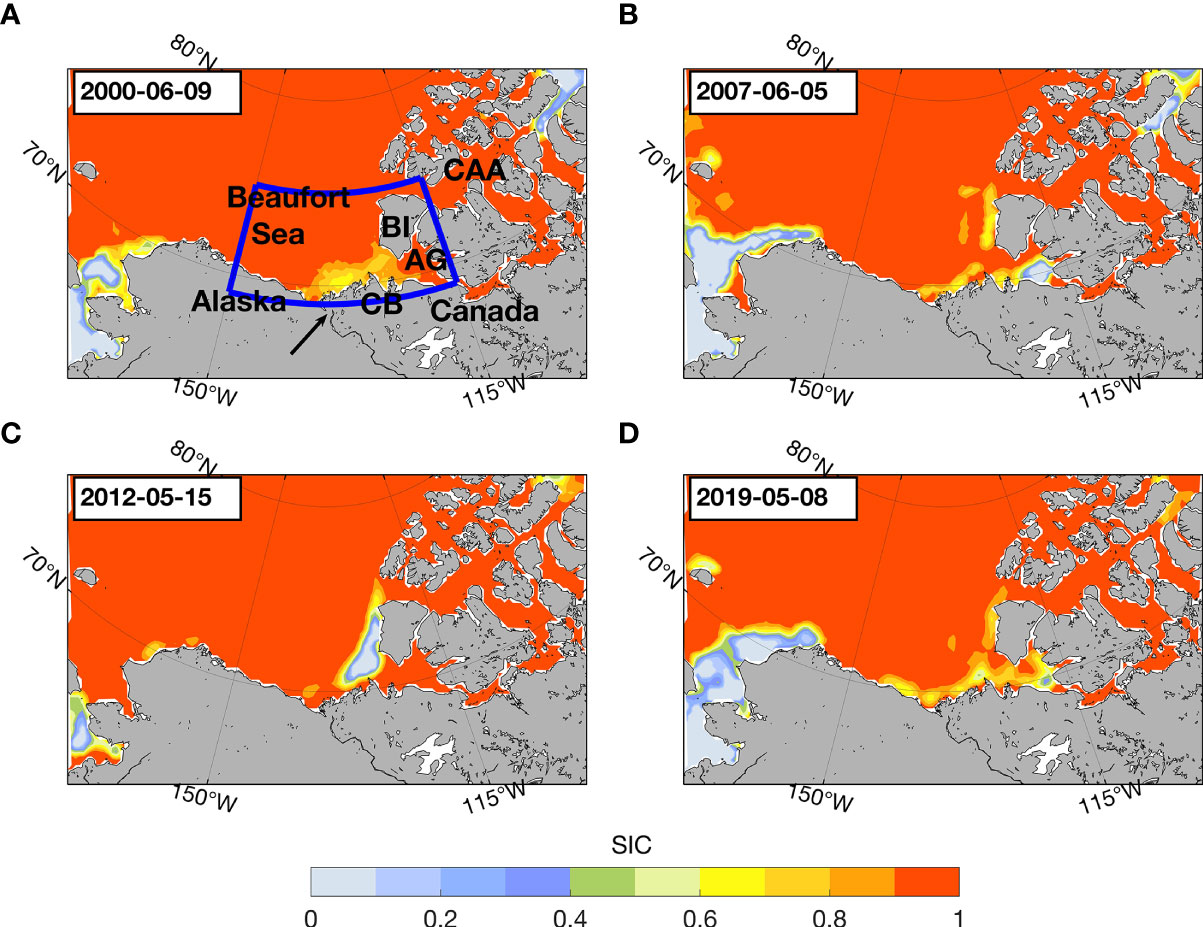
Figure 1 Daily mean ice concentration on (A) 9 June, 2000, (B) 5 June 2007, (C) 15 May 2012, and (D) 8 May 2019. The study domain (69 °N – 75 °N and 115 °W – 150 °W ) is indicated by the blue box. The black arrow represents the western edge of the Mackenzie River delta. Additionally, the Canadian Arctic Archipelago (CAA), Banks Island (BI), Amundsen Gulf (AG), and Cape Bathurst (CB) are shown.

FIGURE 2

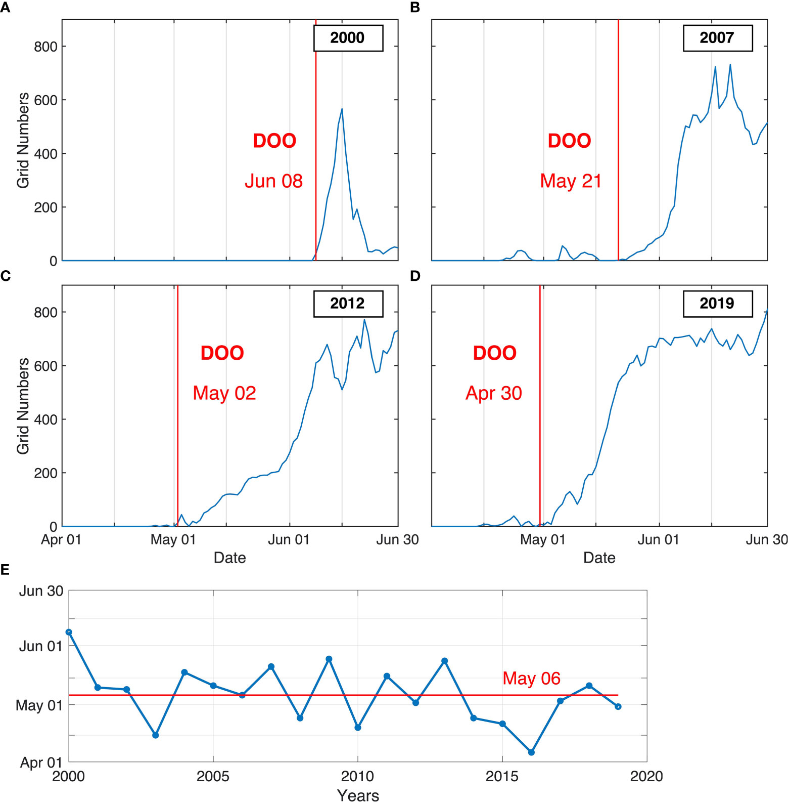
Figure 2 Time series of grid cell numbers with ice concentration lower than 0.8 (blue curve) starting on 1 April in (A) 2000, (B) 2007, (C) 2012, and (D) 2019. The study region is outlined by the blue box in Figure 1A. The red line in (A–D) marks the date of opening (DOO). (E) Interannual variability in DOO during the 2000–2019 period. The red line in (E) indicates the mean DOO (6 May).

3 Results

The DOO exhibits obvious interannual variability ranging from April to June, with the earliest breakup on 6 April 2016, and the latest breakup on 8 June 2000 (Figure 2E). The mean DOO in the Beaufort Sea over the 2000–2019 period is 6 May. To figure out the synoptic weather pattern that triggers the spring ice opening in the Beaufort Sea, we perform a composite analysis from 10 days prior to the DOO (DOO-10) to 10 days after the DOO (DOO+10) over the 20-year period.

Figure 3 shows the composite SIC for subsequent days after the DOO. Some grid cells of sustained ice reduction appear in the shelf and slope regions along northwestern Canada and in the eastern limit of the Amundsen Gulf on DOO+2. From DOO+2 to DOO+12, the area of ice reduction expands gradually, forming a broad area of reduced ice concentration in the southeastern Beaufort Sea where the Cape Bathurst Polynya exists during winter.

FIGURE 3

Figure 3 Composite SIC after the DOO.

3.1 Synoptic-scale variability in the Beaufort High around the DOO

Figure 4A shows the composite SLP and surface winds from DOO-7 to DOO+4. On DOO-7, there is a broad BH over the Chukchi and Beaufort Seas and a weak AL over the Aleutian Islands. In the following few days, the BH shifts eastward from the Chukchi Sea to the west of the Canadian Archipelago. As it shifts eastward, the BH strengthens, narrows west-to-east, stretches north-to-south, and extends further to the south. Simultaneously, the AL strengthens and expands in size with its center located between the East Asian coast and the west North American coast. This prevailing synoptic weather pattern leads to a strong pressure gradient between the two systems and induces offshore winds (southeasterly) from the Alaskan and Canadian coasts to the Arctic Ocean. Such an SLP pattern and wind regime persist for nearly 2 weeks and are believed to be responsible for spring ice loss in the Beaufort Sea.

FIGURE 4

Figure 4 (A) Composite SLP (hPa, color) and 10 m wind vector (m s⁻¹, black arrows) during the ice opening process (from DOO-7 to DOO+4) for the 2000–2019 period. (B) Composite time series of SIC and zonal (u) and meridional (v) wind speed components averaged over the region outlined in Figure 1A (the land area is masked out). Easterly and northerly winds are assigned negative values.

The average surface wind over the study domain changes from a weak, northwesterly wind to a strong, southeasterly wind around DOO+3. The meridional component is weak (approximately 1 m s⁻¹), and the zonal component is strong (approximately 4 m s⁻¹) (the winds persist from the southeast out to DOO+10). The average SIC decreases remarkably 3 days after surface wind changes (Figure 4B).

3.2 Sea ice circulation changes

The eastward shift of the BH induces significant changes in the sea ice circulation in the Beaufort Sea, as shown in Figure 5. Before the shift of the BH, there is a roughly symmetrical anticyclonic sea ice circulation in the Beaufort Sea, i.e., the Beaufort Gyre. The gyre advects sea ice through the Beaufort Sea, with thicker ice from the central Arctic being imported from the north, and thicker ice in the Beaufort being advected westward towards the Chukchi. After DOO-3, in association with the eastward-shifted and strengthened BH (see Figure 4A), the anticyclonic sea ice circulation becomes an asymmetrical gyre that northern import is cutoff and westward transport leads to divergence. This dynamic process is favorable for sea ice loss in the eastern Beaufort Sea.

FIGURE 5

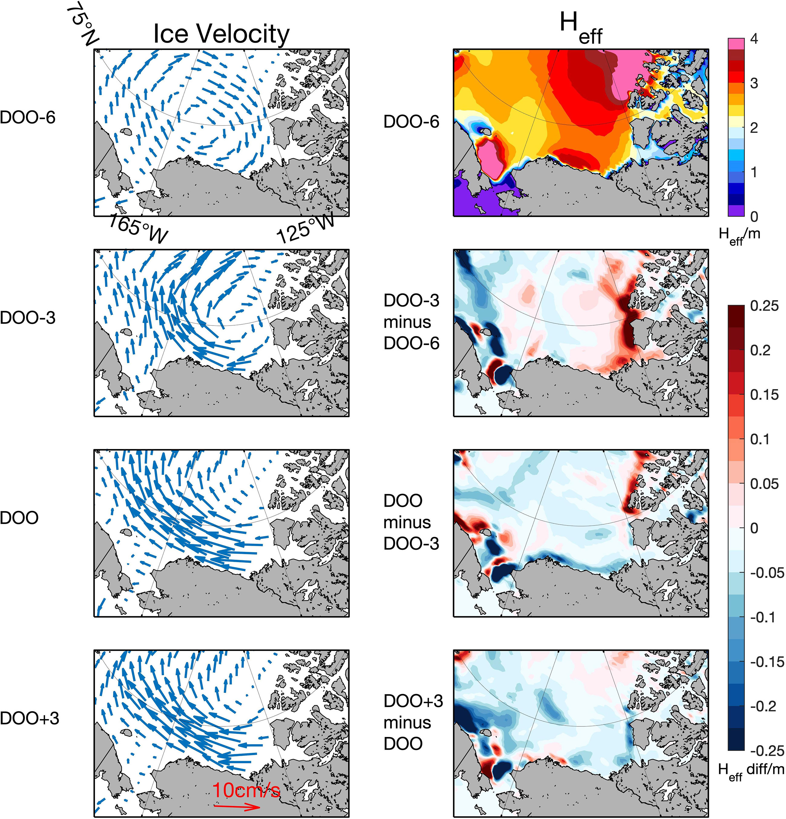
Figure 5 Composite ice velocity on DOO-6, DOO-3, DOO, and DOO+3 for the 2000–2019 period (left column). Composite effective sea ice thickness (H_eff) on DOO-6 and changes in H_eff thereafter (right column).

3.3 Sea ice volume budget

Decomposition of the sea ice volume change (or thickness change) helps to quantify thermodynamic versus dynamical influences (see details in Appendix A). Figure 6 presents the volume budget components calculated using PIOMAS H_eff and NSIDC sea ice velocity prior to, at the start of, and at the peak of the southeasterly winds. The intensification means the change rate of ice volume (i.e., ∂V/∂t ) and the residual term is calculated by ∂V/∂t−D , where D is a combination of ice advection and divergence.

FIGURE 6

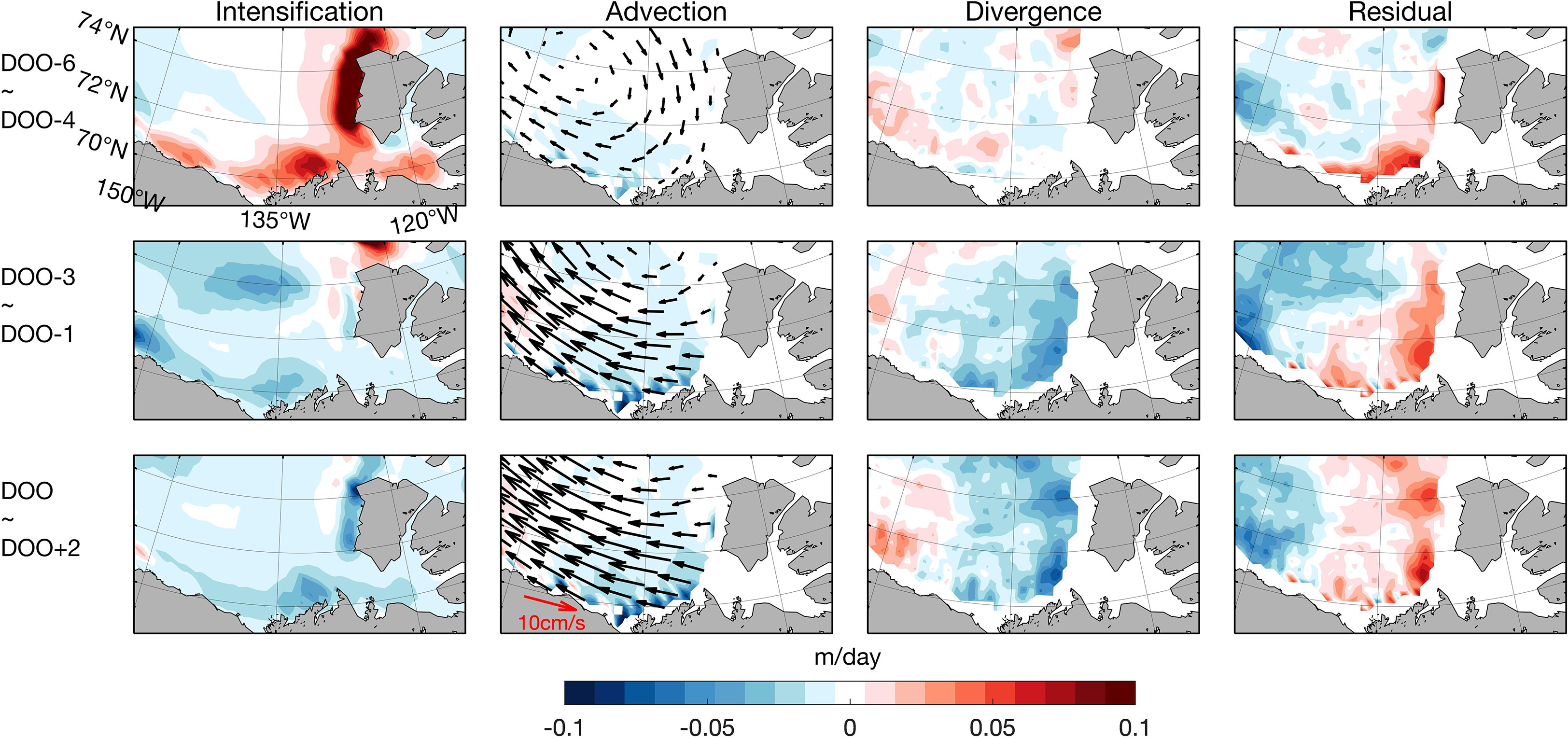
Figure 6 Sea ice volume budget components, including (left to right) intensification, advection, divergence, and residual terms (top) prior to (DOO-6 to DOO-4), at the start of (DOO-3 to DOO-1), and during the peak of southeasterly winds (DOO to DOO+2). Units are m day⁻¹. Blue (red) values indicate a decrease (increase) in sea ice volume.

The budget components show obvious differences before and after the burst of southeasterly winds that began on DOO-3 (Figure 6). The intensification rate prior to the burst of southeasterly winds (DOO-6 to DOO-4) shows an ice volume increase along the west coast of Banks Island and Alaska’s north coast. This increase is partly explained by the ice convergence, while the residual term is the most pronounced, indicating that thermodynamics dominates the ice growth. Note, however, that the residual term obtained by subtracting the dynamic contribution from the ice volume change must accumulate errors of the data and calculation, and this is likely to cause an overestimate of the thermodynamic contribution (see the estimated growth/melt rates in Section 3.4). After the burst of the southeasterly winds (DOO-3 to DOO-1), the ice volume increase along the west coast of Banks Island disappears, and the ice volume decreases in the central Canada Basin and along the Alaskan coast. Obvious net divergence and westward advection lead to a slight increase in ice volume in the western Beaufort Sea and a decrease in the eastern Beaufort Sea. Following breakup (DOO to DOO+2), both divergence and advection strengthen and contribute to a further ice volume decrease in the southeastern Beaufort (bottom row of Figure 6), where breakup occurs (see Figure 3).

3.4 Ice melting under the influence of southerly winds

As mentioned above in Section 3.3, the residual term represents the effect of thermodynamics and the accumulation of errors from the other calculations. To better evaluate the thermodynamic contribution to the ice volume loss around the DOO, we present changes in surface radiation fluxes and calculate the basal and lateral melt rates.

In association with the enhanced BH with less cloudiness, the surface net shortwave radiation (Q_SW) increases significantly in the southern and eastern Beaufort Sea, while the net longwave radiation (Q_LW) increases slightly, indicating that the changes in the surface net radiation flux (Q_Net) are mainly attributed to shortwave radiation (Figure 7A). The domain-averaged Q_SW and Q_Net increase considerably starting on DOO-3. The Q_SW increases from ~40 W m⁻² on DOO-10 to ~75 W m⁻² on DOO+10, and the Q_Net increases from ~5 W m⁻² on DOO-10 to ~40 W m⁻² on DOO+10 (Figure 7B, a positive value means a downward heat flux from the atmosphere to surface).

FIGURE 7

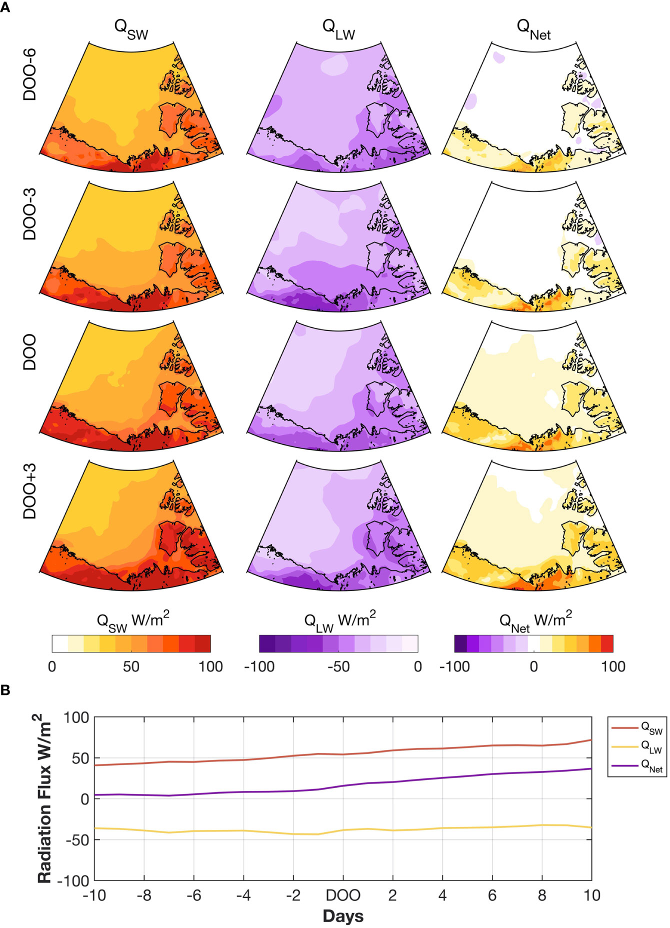
Figure 7 (A) Composite surface net shortwave radiation flux Q_SW (the left column), surface net longwave radiation flux Q_LW (the middle column), and surface net radiation flux Q_Net (the right column) on DOO-6, DOO-3, DOO, and DOO+3 for the 2000–2019 period. Q_Net = Q_SW + Q_LW. The units of all are W m⁻², and positive (negative) values indicate a downward (upward) flux. (B) Composite time series of Q_SW, Q_LW, and Q_Net averaged over the region outlined in Figure 1A (the land area is masked out).

The SAT in the Beaufort Sea increases (left column in Figure 8A) owing to the offshore advection of warm air (see the wind fields in Figure 4A). The ice temperature (IST and IBT) also increases due to atmospheric heating, while the change in SST is not significant (Figure 8A). Similar to SAT, the increases in the IST and IBT progress northwards, mimicking the coastline of northern Alaska and Canada. Although the average IST increases from −9°C on DOO-10 to −3°C on DOO+10 (Figure 8B), all temperature values in the Beaufort Sea remain below 0°C (Figure 8A). Thus, ice top surface melting does not occur during the ice opening process [according to Eq. (2) in Appendix A].

FIGURE 8

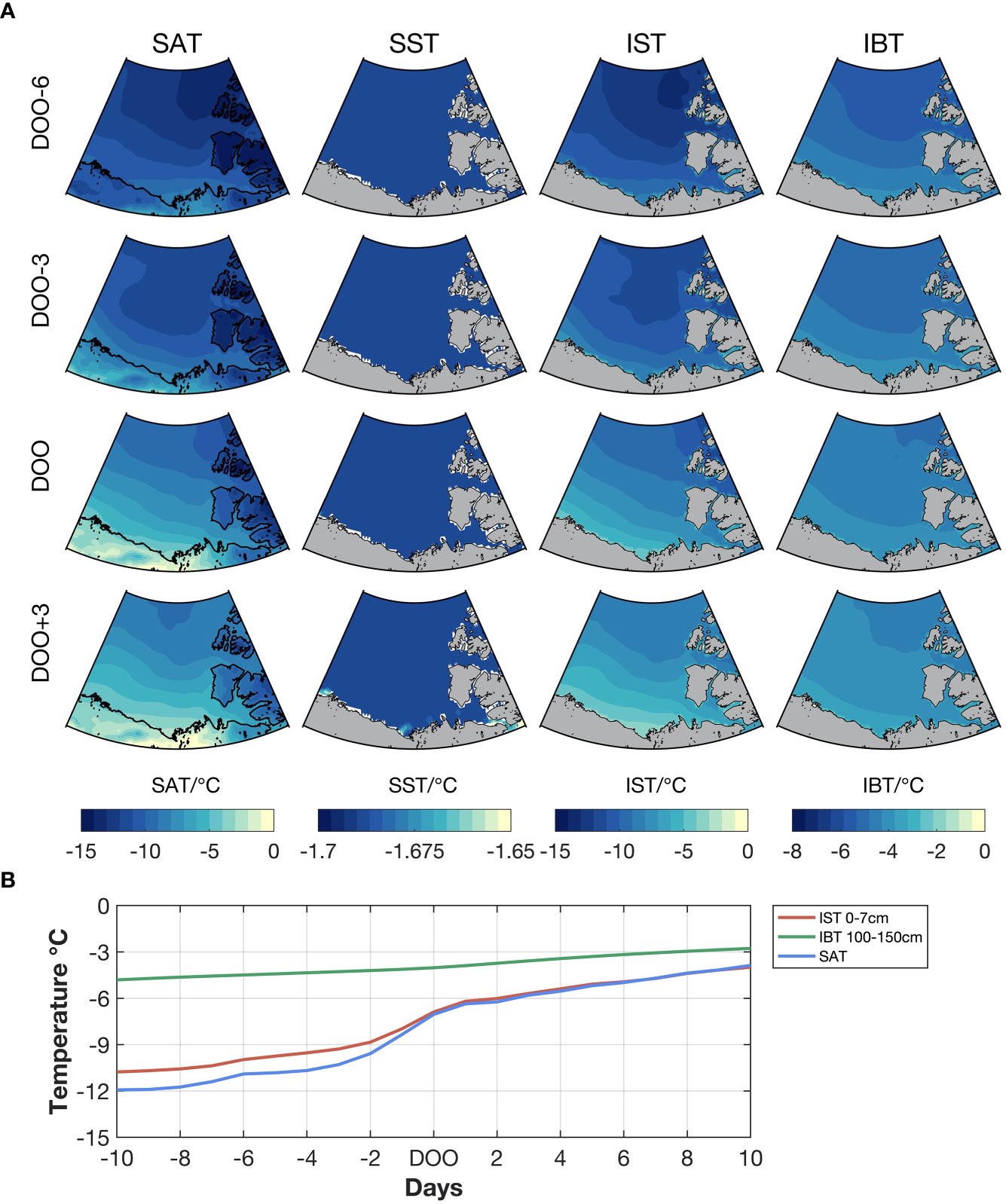
Figure 8 (A) Composite 2-m air temperature (SAT) (first column), sea surface temperature (SST) (second column), ice surface temperature (IST) (third column), and ice bottom temperature (IBT) (last column) on DOO-6, DOO-3, DOO, and DOO+3. The units of all are °C . (B) Composite time series of SAT and ice temperature in the top and bottom layers averaged over the region outlined in Figure 1A (the land area is masked out).

According to Eq. (3) in Appendix A, the decrease in ice thickness (∂H/∂t)|_basal due to basal melting depends on the difference of heat flux from the ocean to the ice F_OI and upward conductive heat flux through the ice column −k(∂T/∂z) . For simplicity, the term F_OI is taken to be 5 W m⁻², which is the representative value for spring (April to May) estimated by Perovich et al. (1997). ∂T/∂z is estimated by (IST−IBT)/δz , where δz=121.5 cm is the distance between the center of the surface layer (0–7 cm) and the center of the bottom layer (100–150 cm). During the ice opening process, the IBT is always higher than the IST (Figures 8A, B), which implies a continuous upward conductive heat flux from the bottom to the top of the ice. Both IST and IBT increase due to the warmer air and increased radiation flux, and the increase in IST is much greater than that in IBT (Figure 8B), thus reducing the vertical temperature gradient within ice and hindering the upward conductive heat flux −k(∂T/∂z) . Only when −k(∂T/∂z) is less than 5 W m^−2,will basal melting occur.

The estimated basal growth/melt rates (∂H/∂t)|_basal are shown in Figure 9A. A negative (positive) (∂H/∂t)|_basal indicates ice melting (growth) at the bottom. Sea ice grows throughout the Canadian Basin and Beaufort Sea before the DOO. On and after the DOO, basal ice melting occurs in the coastal sea, with the greatest melting rates near the Mackenzie River delta. On average, the basal growth rate is approximately 1.5×10⁻³ m day⁻¹ before DOO-4 (the red line in Figure 9C). After the southerly wind burst on DOO-3, the growth rate decreases rapidly and changes to a negative value on DOO, indicating the beginning of basal melting. The melt rate continues to increase since DOO and reaches ~0.8×10⁻³ m day⁻¹ on DOO+10.

FIGURE 9

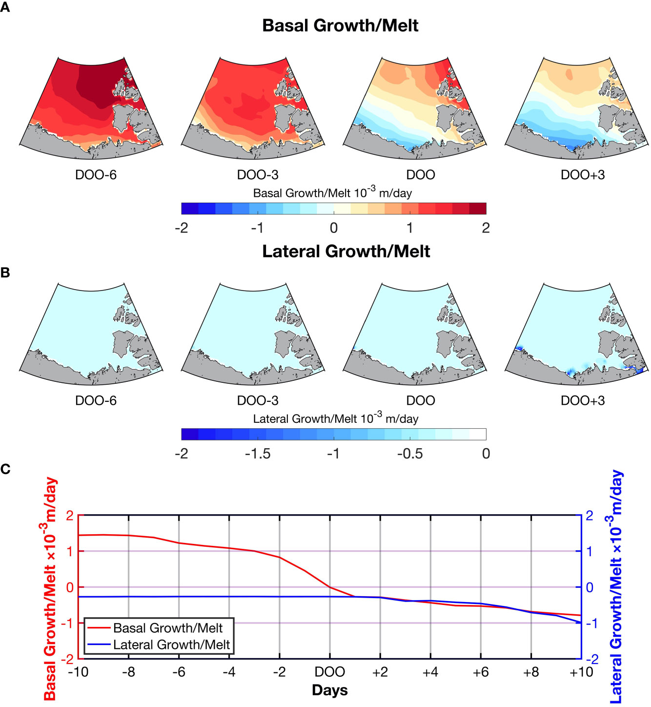
Figure 9 (A) Composite ice growth/melt rate at the bottom of the sea ice on DOO-6, DOO-3, DOO, and DOO+3. (B) Composite lateral melt rate on DOO-6, DOO-3, DOO, and DOO+3. (C) Composite time series of the ice growth/melt rates averaged over the region outlined in Figure 1A (the land area is masked out). A negative (positive) value indicates ice melting (growth).

Eq. (4) in Appendix A means that if the sea surface temperature is higher than the freezing point (taken to be −1.7°C as in ERA-5), lateral ice melt will occur. Before DOO, the SST in the Beaufort Sea is approximately −1.7°C, and the calculated average lateral melting rate is less than 0.3×10⁻³ m day⁻¹ (the blue line in Figure 9C). After DOO, the area of open water occurs along the coastline of Canada and absorbs more solar radiation (Q_SW), leading to a slight rise in sea surface temperature (the second column of Figure 8A). As a response, the lateral melting in coastal areas is promoted and the melt rate reaches 1.0×10⁻³ m day⁻¹ on DOO+10 (Figures 9B, C).

Although both the basal and lateral melting are promoted after DOO, the estimated melt rates are only of order 10⁻³ m day⁻¹, much smaller than the reduction rate of ice volume in the southeastern Beaufort Sea (~ 5×10⁻² m day⁻¹, see Figure 6). This further suggests that wind-forced ice advection and divergence dominate the ice volume loss and drive the ice opening in the Beaufort Sea. The residual term shown in Figure 6 is predominantly the result of errors rather than thermodynamics.

4 Discussion and conclusions

Every spring, the Beaufort Sea’s winter ice cover dynamically breaks up before it begins to melt and thin. Therefore, the timing of breakup that initiates sea ice albedo feedback plays a key role in the following sea ice loss throughout summer. The ice observations from 2000 to 2019 indicate that the mean DOO occurs in early May. The DOO exhibits obvious interannual variability ranging from April to June, with the earliest breakup on 6 April 2016, and the latest breakup on 8 June 2000.

Previous studies have investigated monthly to seasonally averaged ocean–atmosphere contributions to Beaufort Sea ice melt development (Kwok et al., 2013; Frey et al., 2015; Steele et al., 2015), but little is known about synoptic weather systems that stimulate spring ice opening. Our results suggest that synoptic-scale changes in the location, intensity, and shape of the BH are responsible for the spring ice opening in the Beaufort Sea. The composite analysis reveals that during several consecutive days prior to the DOO, the BH strengthens, deforms, and shifts eastward from the Chukchi Sea to the western Canadian Arctic Archipelago, resulting in strong southeasterly winds over the eastern Beaufort Sea and weak northwesterly winds over the Canadian Archipelago (Figure 4A). In association with the eastward-shifted and strengthened BH, there is an immediate response in sea ice motion, and the anticyclonic sea ice circulation in the Canada Basin becomes an asymmetrical gyre with a strong northwestward drift in the west and a very weak southward drift (Figure 5). As a result, sea ice in the eastern Beaufort Sea is exported to the western Beaufort Sea without supplementation from the north. This kind of sea ice circulation pattern causes the ice pack to break up and the formation of open water in the Beaufort Sea.

Advective mechanisms are often used in the literature to explain the spring sea ice loss in the Beaufort Sea (Steele et al., 2015; Lewis and Hutchings, 2019), while thermodynamic effects such as atmospheric heating at the beginning stage of ice loss have not yet been evaluated in previous studies. Based on the composite analysis, we found that as the BH shifts eastward, it also narrows and extends further south (Figure 4A), which promotes southerly winds that transport warm air from the North American continent. Increased atmospheric heating leads to an increase in the ice surface temperature, reduces the temperature gradient within the sea ice, and promotes basal ice melting. After DOO, the area of open water occurs along the coastline of Canada where the lateral melting is promoted. However, both the basal and lateral melt rates are quite small at this stage that they can hardly contribute to the ice breakup in the Beaufort Sea. Sea ice volume budget analysis further illustrates that when southeasterly winds prevail, wind-forced ice advection and divergence dominate the ice volume loss in the Beaufort Sea. Overall, the initial occurrence of breakup is driven by the southeasterly winds, and once there is open water, thermodynamics begins to melt the ice pack and amplifies ice loss via the ice albedo feedback throughout summer.

It is evident now that the location of the BH is important in the prediction of ice opening in the Beaufort Sea. However, the synoptic analysis provides only a short lead time for the prediction since the ice in the Beaufort Sea decreases immediately in response to the eastward movement of the BH. Combining SIC and wind fields, we also find that the earlier (later) DOO in the Beaufort Sea corresponds to the stronger (weaker) BH and AL in April (not shown). This suggests that, once a clear relationship between the DOO and the monthly BH and AL magnitude is established, it will be possible to predict the DOO 1 month in advance.

Data Availability Statement

Publicly available datasets were analyzed in this study. This data can be found here: The NSIDC sea ice concentration data are available at https://doi.org/10.7265/N59P2ZTG. The NSIDC sea ice motion vectors are available at https://doi.org/10.5067/INAWUWO7QH7B. The PIOMASS sea ice thickness data are available at http://psc.apl.uw.edu/research/projects/arctic-seaice-volume-anomaly/data/model_grid. The ERA-5 hourly data on single levels are available at https://cds.climate.copernicus.eu/cdsapp#!/dataset/10.24381/cds.adbb2d47. The ERA5 monthly averaged data on pressure levels are available at https://cds.climate.copernicus.eu/cdsapp#!/da taset/10.24381/cds.6860a573.

Author Contributions

YH and XB developed the concept of this study and worked predominantly on the manuscript. HL provided suggestions and contributed to manuscript revision. All authors read and approved the submitted version.

Funding

This work was funded by the National Key Research and Development Program of China (Grant 2017YFA0604600) and the National Natural Science Foundation of China (Grant 41676019).

Acknowledgments

We thank the two reviewers for their helpful comments and suggestions.

Conflict of Interest

The authors declare that the research was conducted in the absence of any commercial or financial relationships that could be construed as potential conflicts of interest.

Publisher’s Note

All claims expressed in this article are solely those of the authors and do not necessarily represent those of their affiliated organizations, or those of the publisher, the editors and the reviewers. Any product that may be evaluated in this article, or claim that may be made by its manufacturer, is not guaranteed or endorsed by the publisher.

Supplementary Material

The Supplementary Material for this article can be found online at: https://www.frontiersin.org/articles/10.3389/fmars.2022.929209/full#supplementary-material

References

Asplin M. G., Fissel D. B., Papakyriakou T. N., Barber D. G. (2015). Synoptic climatology of the southern Beaufort Sea troposphere with comparisons to surface winds. Atmosphere-Ocean 53 (2), 264–281. doi: 10.1080/07055900.2015.1013438

CrossRef Full Text | Google Scholar

Aylmer J., Ferreira D., Feltham D. (2020). Impacts of oceanic and atmospheric heat transports on sea ice extent. J. Climate 33 (16), 7197–7215. doi: 10.1175/JCLI-D-19-0761.1

CrossRef Full Text | Google Scholar

Babb D. G., Landy J. C., Barber D. G., Galley R. J. (2019). Winter sea ice export from the Beaufort Sea as a preconditioning mechanism for enhanced summer melt: A case study of 2016. J. Geophys. Res.-Oceans. 124, 6575–6600. doi: 10.1029/2019JC015053

CrossRef Full Text | Google Scholar

Ballinger T. J., Lee C. C., Sheridan S. C., Crawford A. D., Overland J. E., Wang M. (2019). Subseasonal atmospheric regimes and ocean background forcing of pacific Arctic sea ice melt onset. Clim. Dyn. 52, 5657–5672. doi: 10.1007/s00382-018-4467-x

CrossRef Full Text | Google Scholar

Barber D. G., Hanesiak J. M. (2004). Meteorological forcing of sea ice concentrations in the southern Beaufort Sea over the period 1979 to 2000. J. Geophys. Res. 109, C06014. doi: 10.1029/2003JC002027

CrossRef Full Text | Google Scholar

Barber D. G., Massom R. A. (2007). “The role of Sea ice in Arctic and Antarctic polynyas,” in Polynyas: Windows to the world ( Netherlands: Elsevier), 1–54. doi: 10.1016/S0422-9894(06)74001-6

CrossRef Full Text | Google Scholar

Bitz C. M., Holland M. M., Hunke E. C., Moritz R. E. (2005). Maintenance of the Sea-ice edge. J. Climate 18, 2903–2921. doi: 10.1175/JCLI3428.1

CrossRef Full Text | Google Scholar

Cavalieri D. J., Gloersen P., Campbell W. J. (1984). Determination of Sea ice parameters with the NIMBUS-7 SMMR. J. Geophys. Res. 89, 5355–5369. doi: 10.1029/JD089iD04p05355

CrossRef Full Text | Google Scholar

Comiso J. C. (1986). Characteristics of Arctic winter sea ice from satellite multispectral microwave observations. J. Geophys. Res. 91, 975–994. doi: 10.1029/JC091iC01p00975

CrossRef Full Text | Google Scholar

Frey K. E., Moore G. W. K., Cooper L. W., Grebmeier J. M. (2015). Divergent patterns of recent sea ice cover across the Bering, chukchi, and Beaufort seas of the pacific Arctic region. Prog. Oceanogr. 136, 32–49. doi: 10.1016/j.pocean.2015.05.009

CrossRef Full Text | Google Scholar

Galley R. J., Babb D., Ogi M., Else B. G. T., Geilfus N. X., Crabeck O., et al. (2016). Replacement of multiyear sea ice and changes in the open water season duration in the Beaufort Sea since 2004. J. Geophys. Res.-Oceans. 121, 1806–1823. doi: 10.1002/2015JC011583

CrossRef Full Text | Google Scholar

Hersbach H., Bell B., Berrisford P., Biavati G., Horányi A., Muñoz Sabater J., et al. (2018). “Copernicus Climate change service (C3S) climate data store (CDS),” in ERA5 hourly data on single levels from 1979 to present. doi: 10.24381/cds.adbb2d47

CrossRef Full Text | Google Scholar

Hersbach H., Bell B., Berrisford P., Biavati G., Horányi A., Muñoz Sabater J., et al. (2019). “Copernicus Climate change service (C3S) climate data store (CDS),” in ERA5 monthly averaged data on pressure levels from 1979 to present. doi: 10.24381/cds.6860a573

CrossRef Full Text | Google Scholar

Holland M. M., Bitz C. M., Tremblay B. (2006). Future abrupt reductions in the summer Arctic sea ice. Geophys. Res. Lett. 33, L23503. doi: 10.1029/2006GL028024

CrossRef Full Text | Google Scholar

Kwok R., Spreen G., Pang S. (2013). Arctic Sea ice circulation and drift speed: Decadal trends and ocean currents. J. Geophys. Res.-Oceans. 118, 2408–2425. doi: 10.1002/jgrc.20191

CrossRef Full Text | Google Scholar

Lewis B. J., Hutchings J. K. (2019). Leads and associated sea ice drift in the Beaufort Sea in winter. J. Geophys. Res.: Oceans. 124, 3411–3427. doi: 10.1029/2018JC014898

CrossRef Full Text | Google Scholar

Lukovivh J. V., Stroeve J. C., Crawford A., Hamilton L., Tsamaods M., Heorton H., et al. (2021). Summer extreme cyclone impacts on Arctic Sea ice. J. Climate 34, 4817–4834. doi: 10.1175/JCLI-D-19-0925.1

CrossRef Full Text | Google Scholar

Maykut G. A., McPhee M. G. (1995). Solar heating of the Arctic mixed layer. J. Geophys. Res.-Oceans. 100, 24691–24703. doi: 10.1029/95JC02554

CrossRef Full Text | Google Scholar

Meier W. N., Fetterer F., Savoie M., Mallory S., Duerr R., Stroeve J. (2017). NOAA/NSIDC climate data record of passive microwave Sea ice concentration, version 3 (Boulder, Colorado USA: NSIDC: National Snow and Ice Data Center). doi: 10.7265/N59P2ZTG

CrossRef Full Text | Google Scholar

Nghiem S. V., Hall D. K., Rigor I. G., Li P., Neumann G. (2014). Effects of Mackenzie river discharge and bathymetry on sea ice in the Beaufort Sea. Geophys. Res. Lett. 41, 873–879. doi: 10.1002/2013GL058956

CrossRef Full Text | Google Scholar

Peng G., Meier W. N., Scott D. J., Savoie M. H. (2013). A long-term and reproducible passive microwave sea ice concentration data record for climate studies and monitoring. Earth Syst. Sci. Data 5, 311–318. doi: 10.5194/essd-5-311-2013

CrossRef Full Text | Google Scholar

Perovich D. K. (1983). On the summer decay of a sea ice cover. Ph.D. dissertation# ( Seattle: University of Washington).

Google Scholar

Perovich D. K., Bruce C. E., Jacqueline A. R.-M. (1997). Observations of the annual cycle of sea ice temperature and mass balance. Geophys. Res. Lett. 24, 555–558. doi: 10.1029/97GL00185

CrossRef Full Text | Google Scholar

Perovich D. K., Elder B. (2002). Estimates of ocean heat flux at SHEBA. Geophys. Res. Lett. 29(9), 1344. doi: 10.1029/2001GL014171

CrossRef Full Text | Google Scholar

Perovich D. K., Polashenski C. (2012). Albedo evolution of seasonal Arctic sea ice. Geophys. Res. Lett. 39, L08501. doi: 10.1029/2012GL051432

CrossRef Full Text | Google Scholar

Petty A. A., Hutchings J. K., Richter-Menge J. A., Tschudi M. A. (2016). Sea Ice circulation around the Beaufort gyre: The changing role of wind forcing and the sea ice state. J. Geophys. Res.-Oceans. 121, 3278–3296. doi: 10.1002/2015JC010903

CrossRef Full Text | Google Scholar

Proshutinsky A., Bourke R. H., McLaughlin F. A. (2002). The role of the Beaufort gyre in Arctic climate variability: Seasonal to decadal climate scales. Geophys. Res. Lett. 29, 2100. doi: 10.1029/2002gl015847

CrossRef Full Text | Google Scholar

Rigor I. G., Wallace J. M. (2004). Variations in the age of Arctic sea-ice and summer sea-ice extent. Geophys. Res. Lett. 31, L09401. doi: 10.1029/2004GL019492

CrossRef Full Text | Google Scholar

Schweiger A., Lindsay R., Zhang J., Steele M., Stern H., Kwok R. (2011). Uncertainty in modeled Arctic sea ice volume. J. Geophys. Res. 116, C00D06. doi: 10.1029/2011JC007084

CrossRef Full Text | Google Scholar

Serreze M. C., Barrett A. P. (2011). Characteristics of the Beaufort Sea high. J. Climate 24, 159–182. doi: 10.1175/2010JCLI3636.1

CrossRef Full Text | Google Scholar

Serreze M. C., Crawford A. D., Stroeve J. C., Barrett A. P., Woodgate R. A. (2016). Variability, trends, and predictability of seasonal sea ice retreat and advance in the chukchi Sea. J. Geophys. Res. Oceans. 121, 7308–7325. doi: 10.1002/2016JC011977

CrossRef Full Text | Google Scholar

Steele M., Dickinson S., Zhang J., Lindsay R. (2015). Seasonal ice loss in the Beaufort Sea: Toward synchrony and prediction. J. Geophys. Res.-Oceans. 120, 1118–1132. doi: 10.1002/2014JC010247

CrossRef Full Text | Google Scholar

Stroeve J., Notz D. (2018). Changing state of Arctic sea ice across all seasons. Environ. Res. Lett. 13, 103001. doi: 10.1088/1748-9326/aade56

CrossRef Full Text | Google Scholar

Stroeve J., Serreze M., Holland M., Kay J., Malanik J., Barrett A. (2012). The arctic's rapidly shrinking sea ice cover: A research synthesis. Clim. Change 110 (3-4), 1005–1027. doi: 10.1007/s10584-011-0101-1

CrossRef Full Text | Google Scholar

Tschudi M., Meier W. N., Stewart J. S., Fowler C., Maslanik J. (2019). Polar pathfinder daily 25 km EASE-grid Sea ice motion vectors, version 4 (Boulder, Colorado USA: NASA National Snow and Ice Data Center Distributed Active Archive Center). doi: 10.5067/INAWUWO7QH7B

CrossRef Full Text | Google Scholar

Zhang J., Liu F., Tao W., Krieger J., Shulski M., Zhang X. (2016). Mesoscale climatology and variation of surface winds over the chukchi–Beaufort coastal areas. J. Clim. 29 (8), 2721–2739. doi: 10.1175/JCLI-D-15-0436.1

CrossRef Full Text | Google Scholar

Zhang J., Rothrock D. A. (2003). Modeling global sea ice with a thickness and enthalpy distribution model in generalized curvilinear coordinates. Mon. Wea. Rev. 131, 681–697. doi: 10.1175/1520-0493(2003)131<0845:MGSIWA>2.0.CO;2

CrossRef Full Text | Google Scholar