 Xiaogang Xing
 Zhongping Lee
 Peng Xiu
 Shuangling Chen1
- 1State Key Laboratory of Satellite Ocean Environment Dynamics, Second Institute of Oceanography, Ministry of Natural Resources, Hangzhou, China
- 2State Key Lab of Marine Environmental Science, College of Earth and Ocean Sciences, Xiamen University, Xiamen, China
- 3State Key Laboratory of Tropical Oceanography, South China Sea Institute of Oceanology, Chinese Academy of Sciences, Guangzhou, China
- 4Guangdong Key Laboratory of Ocean Remote Sensing, South China Sea Institute of Oceanology, Chinese Academy of Sciences, Guangzhou, China
Based on the optical properties of water constituents, the vertical variation of photosynthetically available radiation (PAR) can be well modeled with hyperspectral resolution; the intensive computing load, however, demands simplified modeling that can be easily embedded in marine physical and biogeochemical models. While the vertical PAR profile in homogeneous waters can now be accurately modeled with simple parameterization, it is still a big challenge to model the PAR profile in stratified waters with limited variables. In this study, based on empirical equations and simulations, we propose a dual-band model to characterize the vertical distribution of PAR using the chlorophyll concentration (Chl). With an inclusive dataset including cruise data collected in the Southeast Pacific and BGC-Argo data in the global ocean, the model was thoroughly evaluated for its general applicability in three aspects: 1) estimating the entire PAR profile from sea-surface PAR and the Chl profile, 2) estimating the euphotic layer depth from the Chl profile, and 3) estimating PAR just below the sea surface from in situ radiometry measurements. It is demonstrated that the proposed dual-band model is capable of generating similar estimates as that from a hyperspectral model, thus offering an effective module that can be incorporated in large-scale ecosystem and/or circulation models for efficient calculations.
Introduction
The diurnal and seasonal cycles of solar radiation and its underwater vertical distribution play an important role in ocean heat uptake (Lewis et al., 1990), which impacts sea-surface temperature and upper-ocean stratification (Liang and Wu, 2013; Pimentel et al., 2019; Liu et al., 2020) and in turn acts on ocean circulation (Liang and Wu, 2015) and air–sea interaction (Liu et al., 2021). Moreover, solar radiation also supports primary production and the entire marine ecosystem (Evans and Parslow, 1985; Bryant et al., 2016; Skákala et al., 2020). The visible light part of solar radiation, i.e., photosynthetically available radiation (PAR), is defined as the downwelling photon flux integrated from 400 to 700 nm. The accuracy of both marine net primary production (NPP) algorithms (Westberry et al., 2008; Fox et al., 2020) and ecosystem models (Skákala et al., 2020) highly depends on the vertical distribution of PAR. Skákala et al. (2020) demonstrated that different PAR attenuation models may result in vastly discrepant phytoplankton seasonal bloom patterns and community structures. Recently, Xing and Boss (2021) illustrated that the use of PAR attenuation models with large uncertainties could lead to an error of 100% of estimated PAR at the half mixed layer depth, which would significantly impact the NPP estimates. PAR attenuation also highly affects the physical oceanography modeling of seawater temperature and mixing (Rochford et al., 2001; Liu et al., 2020; Liu et al., 2021), the diurnal cycles of sea-surface temperature (Pimentel et al., 2019), and even the atmospheric and ocean circulation (Gnanadesikan and Anderson, 2009). For example, Liu et al. (2020) found that the uses of different PAR models would lead to differences up to 1.5°C–2°C in sea surface temperature. An accurate estimate of the PAR profile is the prerequisite to determine the euphotic layer, which is typically used as a proxy for the compensation depth of the phytoplankton ecosystem (Ryther, 1956; Wu et al., 2021). The model-estimated euphotic layer depth is critical not only in carbon export assessment of the ocean biological carbon pump (Carlson et al., 1994; Siegel et al., 2014; Buesseler et al., 2020) but also in marine ecosystem modeling (e.g., Chai et al., 2002; Aumont et al., 2015), as well as in studies on the mechanisms of seasonal phytoplankton blooms (e.g., Behrenfeld, 2010; Mignot et al., 2018).
Accurate estimation of the PAR profile with concise parameterizations has been a serious challenge in the past 50 years (e.g., Lorenzen, 1972; Paulson and Simpson, 1977; Zaneveld and Spinrad, 1980; Byun et al., 2014). Most of the difficulty lies in the combined effects of two characteristics of the propagation of solar radiation in water: the strong and spectrally selective attenuation near the sea surface and the quasi-inherent optical property (IOP) characteristics of the blue-green band in open oceanic waters. The former is related to the faster attenuation in the longer wavelengths due to the strong absorption by water molecules (Paulson and Simpson, 1977; Lee, 2009), while the latter behaves as a correlation of the PAR attenuation to chlorophyll concentration (Chl; Morel, 1988). Therefore, for highly stratified waters where a deep chlorophyll maximum (DCM) exists at the subsurface, the vertical distribution of PAR in the ocean is characterized by two fast-attenuation layers: the first one is near the sea surface related to the fast loss of red light (Paulson and Simpson, 1977; Lee, 2009), and the second one is around the DCM, as a result of enhanced absorption and backscattering by phytoplankton (Xing and Boss, 2021). It is not surprising that the parameterization scheme of PAR based on homogeneous IOPs (Lee et al., 2005) cannot accurately estimate the attenuation around DCM (Xing and Boss, 2021), as the IOPs vary with depth (Bricaud et al., 2010). The entire profile of IOPs or Chl, therefore, is required for the simulation of PAR profiles in stratified waters. Recently, Xing and Boss (2021) proposed a chlorophyll-profile-based parameterization scheme, termed “GCMM.” This scheme combines the clear-sky spectral irradiance model of Gregg and Carder (1990) (GC90) and the empirical spectral relationships between Chl and the spectral diffuse attenuation coefficients (Kd) developed by Morel and Maritorena (2001) (MM01). With the Chl profile as input and a hyperspectral resolution, the scheme solves well the combined effects of spectral selectivity and quasi-IOP characteristics.
Although the GCMM model showed good performance in estimating PAR profiles in stratified waters (Xing and Boss, 2021), it needs hyperspectral processing, i.e., decomposing PAR to spectral irradiance with a wavelength resolution of 1 nm. As a result, the computing load is very high, particularly when implementing in ecosystem models or global gridded datasets. Recently, Lee et al. (2014) have proposed the concept of usable solar radiation (USR), which focused on the irradiance or photon flux in the 400–560-nm domain. The merits of USR are that it is not influenced by the fast attenuation at longer wavelengths, and the attenuation of USR is highly sensitive to phytoplankton. Therefore, based on the characteristics of USR attenuation, in this study, we propose a dual-band PAR parameterization model that decomposes PAR into two wide bands, USR (400–560 nm) and Green-to-Red (GR, 560–700 nm). Such a processing of splitting the whole PAR domain to two or three bands has been used before in some regional models (e.g., Fasham et al., 1983; Zielinski et al., 2002; Wollschläger et al., 2020). Our proposed model, termed USRGR, has a simplified parameterization compared to the hyperspectral GCMM scheme but delivers equivalent performances in estimating the PAR profile in stratified waters. This model is applicable not only to estimate the euphotic layer depth and daily PAR profile from in situ Chl measurements, and sea-surface PAR from underwater PAR observations, but also to ecosystem or general circulation models that require daily or hourly PAR profiles to drive the phytoplankton growth or upper-layer water temperature change.
Materials and Methods
Model Structure
To model a PAR profile with a Chl profile as the input, the procedures and components of USRGR (Figure 1) include the following:
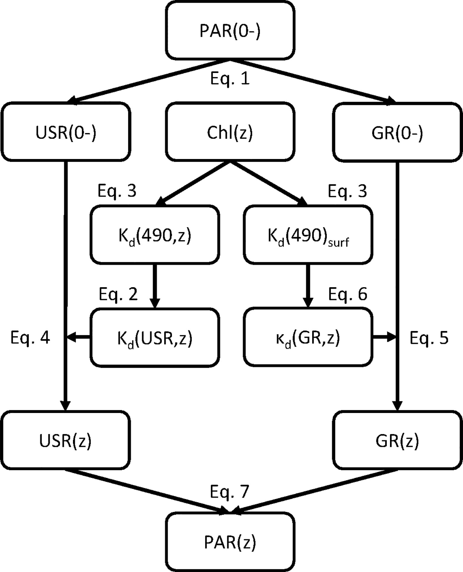
Figure 1 Structure of the USRGR model.
1) The sea-surface PAR(0-) is decomposed into two bands (Eq. 1), USR and GR, via the relative measure (represented as β) of USR(0-) out of PAR(0-), which can be determined from the latitude and day of year (see the look-up table made through the GC90 model1). β is around 0.48 for the quanta unit (e.g., μmol photons m-2 s-1) and around 0.55 for the irradiance unit (e.g., W m-2), with a slight dependence on the solar zenith angle.
2) A given Chl profile is interpolated into a fine resolution at an interval of 1 m (1 m, 2 m, 3 m, etc.);
3) Kd(USR,z) is modeled as a function of Kd(490,z) (Eq. 2; Lin et al., 2016), with Kd(490,z) at each depth z determined with the Chl–Kd empirical relationship of MM01 (Eq. 3);
Here this Chl–Kd relationship represents a nominal solar-zenith angle ~40°. For situations of extremely high or low sun angles, an adjustment is necessary if higher accuracy is desired.
4) USR is vertically attenuated with Kd(USR,z) layer by layer (Eq. 4):
For z = 1 m, (z-1) represents the sea surface (0-);
5) A layer-averaged diffuse attenuation coefficient (κd) is used for the propagation of the GR band from the surface to any depth (Eq. 5):
Note that κd here represents the averaged diffuse attenuation coefficient from the surface (0-) to any given depth (z), while Kd of Eq. 4 represents the diffuse attenuation coefficient at the given depth (z). We use the layer-averaged one here because the light attenuation of GR mainly depends on the pure-water absorption For Chl in a range of 0.02 to 2.0 mg/m3 (100 data points, ~4% increase rate), through numerical simulations of Hydrolight (Mobley, 1995), it is found that κd(GR) can be approximated as:
Here, Kd(490)surf is derived from Eq. 3 using averaged Chl within z ≤ 10 m.
6) Finally, PAR at each depth (PAR(z)) is obtained as a sum of USR(z) and GR(z):
Applications of the USRGR Model
Figure 2 illustrates three applications of the USRGR model, with the first one to estimate daily PAR profiles. Its required inputs include the observed or modeled Chl profile and sea-surface daily PAR(0-) from ocean-color satellites (e.g., MODIS-Aqua) or reanalysis products (e.g., ECMWF-ERA). It is applicable with vertical Chl observations obtained from in situ platforms (e.g., research vessel, BGC-Argo, and underwater glider), global gridded Chl profile datasets (e.g., Sauzède et al., 2016), and ecosystem models with the Chl profile as a product (e.g., Fennel et al., 2006; Fujii et al., 2007). The corresponding Matlab function can be found in GitHub2. For observation data, the derived PAR profile can be further employed to estimate net primary production, through the Carbon-based Production Model (CbPM; Westberry et al., 2008), Photoacclimation-based Production Model (PbPM; Fox et al., 2020), or Absorption-based Model (AbPM; Lee et al., 1996; Lee et al., 2015); for ecosystem models, the derived PAR profile can be used to initiate the process of photosynthesis and then drive the phytoplankton growth and Chl change. The dynamics of phytoplankton biomass would in turn adjust the light penetration via bio-optical feedbacks (Manizza et al., 2005).
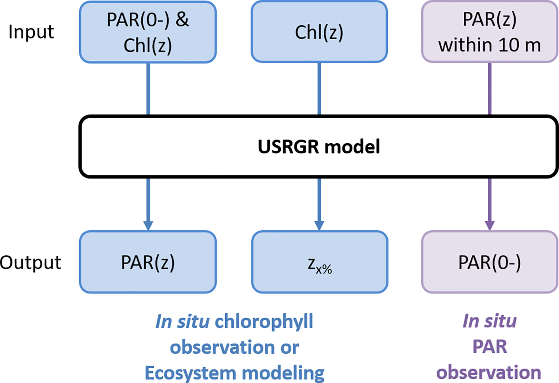
Figure 2 Applications of the USRGR model. zx% represents the depth where PAR is attenuated to 1% (z1%; Ryther, 1956) or 0.5% of sea-surface value (z0.5%; Wu et al., 2021).
Second, the euphotic layer depth, defined as the depth where PAR is attenuated to 1% (z1%; Ryther, 1956) or 0.5% of sea-surface value (z0.5%; Wu et al., 2021), can be derived directly through the USRGR model from a Chl profile (Figure 2). In this case, the sea-surface PAR is not required, as the euphotic layer depth refers to the relative change of PAR in the water column, which actually represents the transmittance of PAR. From the model structure of the USRGR (Eqs. 1, 4, 5, and 6), it is clear that the transmittance of PAR mainly relies on Kd(490,z), which is further expressed as a function of Chl. As such, the percentage PAR profile (i.e., a relative PAR profile normalized by sea-surface PAR) can be directly calculated from the corresponding Chl profile, and then the euphotic layer depth would be determined.Third, the USRGR model can also be used to obtain sea-surface PAR(0-) from underwater radiometry observations (e.g., a radiometry profiler conducted on a research vessel or a BGC-Argo float with downwelling PAR observation). It should be clarified, although the PAR profile can be measured in situ, that it is rarely possible to measure PAR close to z = 0-, owing to surface waves. As such, PAR(0-) has to be estimated from downwelling irradiance observed above the sea surface or by upward extrapolation from downwelling irradiance within the water column. However, the above-surface observation is not always available, e.g., from the BGC-Argo floats. The USRGR model can be employed to extrapolate PAR(0-) from the underwater PAR profile based on the bio-optical relationships. In natural waters, it is reasonable to assume a homogeneous distribution of IOPs and Chl within the surface layer (like ≤10 m) due to the surface mixing effect. Within this layer, therefore, Chl can be regarded as a depth-independent variable. Then the USRGR model could express the PAR profile within the 10-m layer with only two variables: PAR(0-) and Chl. As such, it would be straightforward to derive PAR(0-) via an optimization analysis on the PAR profile (Figure 2). The derived PAR(0-) can be further employed to calculate the layer-averaged diffuse attenuation coefficient from the surface to any depth (Xing et al., 2020).It should be noted that all three applications (estimation of the PAR profile, euphotic depth, and sea-surface PAR) are not exclusive to the USRGR model but can also be achieved by some other PAR attenuation models. In this study, we evaluate the USRGR model through these applications, to demonstrate that the USRGR model can tackle these questions with similar quality (i.e., performance) as the previous models (e.g., hyperspectral), but with efficient computation.
Data
In this study, we evaluate the performance of the USRGR model against two in situ datasets: the first one is the ship-borne measurements collected from the Biogeochemistry and Optics South Pacific Experiment (BIOSOPE) cruise (Claustre et al., 2008). The cruise was conducted in the Southeast Pacific between October and December 2004 (Supplementary Figure 1). A total of 39 spectral-irradiance profiles were recorded by a Satlantic profiler, and the corresponding surface irradiance measurements were obtained by a Satlantic TSRB (Tethered Spectral Radiometer Buoy). The radiometry data covered various trophic conditions, from eutrophic (west of Marquesas Island, and the Chile upwelling) to ultra-oligotrophic (center of South Pacific subtropical gyre). We first conducted a quality-control procedure following Organelli et al. (2016) for all radiometry data to get rid of noisy profiles and data spikes, and 35 profiles remained. The measured irradiance values above the sea surface at each wavelength [Es(λ)] were converted to the ones just below sea surface Ed(0-,λ), by multiplying the air–sea transmission factor α (Mobley and Boss, 2012). Following the MODIS Algorithm Theoretical Basis Document (Carder et al., 2003), the PAR(z) profile and sea-surface PAR(0-) were defined as the integration of photons from 400 to 700 nm (Eq. 8).
where h is Plank’s constant and c is the speed of light in a vacuum. Correspondingly, the observed USR and GR profiles are calculated as:
Chl profile data were measured through collecting discrete water samples quasi-simultaneously to the radiometry and then submitted to the laboratory analysis with high-performance liquid chromatography (HPLC; see Supplementary Text 1).
Despite the accurate Chl measurement and above-water PAR observation, the BIOSOPE cruise only covered a limited area and data samples are not adequate. The second dataset we use is a global BGC-Argo dataset (Supplementary Figure 2), the same as Xing and Boss (2021), to validate the PAR profiles derived from the USRGR model, and to compare the results from the GCMM model. The dataset encompasses 193 BGC-Argo floats in the global open oceans collected from October 2012 to March 2020. All these floats were equipped with Satlantic OCR504 radiometers and Wet Labs ECO in vivo chlorophyll-a fluorometers. The quality control of radiometry followed Organelli et al. (2016), and the correction of Chl fluorometry data were described in Supplementary Text 2.
Besides, as a case application, the monthly climatological Chl profile data, termed SOCA2021 (Sauzède et al., 2021), with a 0.25° horizontal resolution and 36 vertical levels from the surface to 1,000-m depth, provided by the Copernicus Marine Environment Monitoring Service (CMEMS), were used to estimate the euphotic layer depth. This depth-resolved Chl dataset was derived from a neural network model (Sauzède et al., 2016), with inputs including remote-sensing reflectance, daily PAR, and sea-level anomaly from satellites, along with the mixed-layer depth (MLD) product from a reanalysis gridded temperature and salinity dataset (Guinehut et al., 2012).
Statistical Metrics
The statistical metrics used in this study include the root mean square difference (RMSD), mean difference (MD), and mean percentage difference (MPD), defined as:
Here, Mi and Ei are the in situ measured and corresponding model-estimated values, respectively, and n is the number of observations. RMSD represents the total deviations between the measured and estimated values, while MD and MPD represent the absolute and relative system biases of estimated values, respectively.
Results and Discussion
Estimate of the PAR Profile From Sea-Surface PAR and Chl Profile
We first examined the performance of the USRGR model in estimating the PAR profile based on the BIOSOPE cruise data. Figure 3 shows example profiles of observed Chl, PAR, USR, and GR, collected at Station GYR5, in the ultra-oligotrophic center of the Southeast Pacific subtropical gyre (Claustre et al., 2008). At this station, the sea-surface Chl was extremely low (~0.015 mg m-3), and the DCM appeared at 180 m (Figure 3A). The observed USR profile showed a constant attenuation [i.e., close to a straight line in the semi-log coordinate (x-axis as log scale)] near the sea surface but attenuated faster below the depth of ~80 m (Figure 3B), where the corresponding Chl was enhanced (Figure 3A); in contrast, the observed GR profile attenuated very fast near the sea surface and slowed down below ~30 m (Figure 3C), as a result of the fact that all red photons were lost near the surface. Combining USR and GR, we obtained the total PAR profile (Figure 3D). It is clearly observed that there were two fast attenuation layers of the vertical PAR, with the first layer mainly caused by the attenuation in the GR band and the second layer mostly attributed to the enhanced attenuation in the USR band. Overall, the USRGR model performed well to estimate the USR, GR, and total PAR profile, respectively (Figures 3B–D), except for some underestimation of GR below 50 m (Figure 3C), where GR had attenuated to a very low value (<3 μmol photons m-2 s-1). Such an underestimation did not significantly affect the estimation of the PAR profile (Figure 3D). More importantly, compared to the performance of the hyperspectral GCMM model, the dual-band USRGR model resolved similar PAR profiles from the surface to 200 m (Figure 3D).
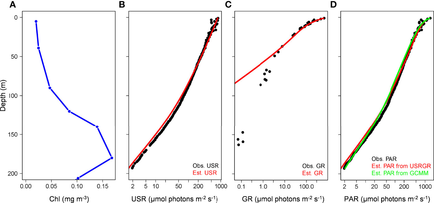
Figure 3 An example of the observed and model-estimated USR, GR, and PAR profiles at Station GYR 5 (26.07°S, 114.02°W) on November 15, 2004 in the Southeast Pacific. (A) Observed Chl based on the HPLC method. (B) Observed USR (black) and estimated one from the USRGR model (red). (C) Observed GR (black) and estimated one from the USRGR model (red). (D) Observed PAR (black) and estimated ones from the USRGR (red) and GCMM model (green), respectively.
Figure 4 shows the statistical results for all the 35 quality-controlled downwelling radiometry profiles observed in the BIOSOPE cruise. All profiles were described using the normalized depth ζ, which was defined as z/z1%. MPD was calculated at each ζ. We found that the estimated USR profiles had quite low MPD values from 0- to 1.5-fold z1% (Figure 4A), except for some slight underestimation around z1%, and the averaged absolute MPD (AMPD) from 0- to 1.5-fold z1% was 8%. The estimated GR profile had a low MPD near the sea surface, and underestimation appeared below ~0.2-fold z1% (Figure 4B), similar to the example profile shown in Figure 3C. Such an underestimation reached maximum around z1%, with MPD close to -100%. However, again, it should be noted that, at such a depth, GR had attenuated to a very low level as mentioned above. As a consequence, the estimated PAR was not affected by the GR underestimation at depth, and its MPD profile displayed a similar vertical pattern to that of the USR (Figures 4A, C), with an AMPD of 9.5%. Compared with the performance of GCMM (AMPD = 12.5%), the USRGR model demonstrated similar and even better performance in estimating the PAR profile.
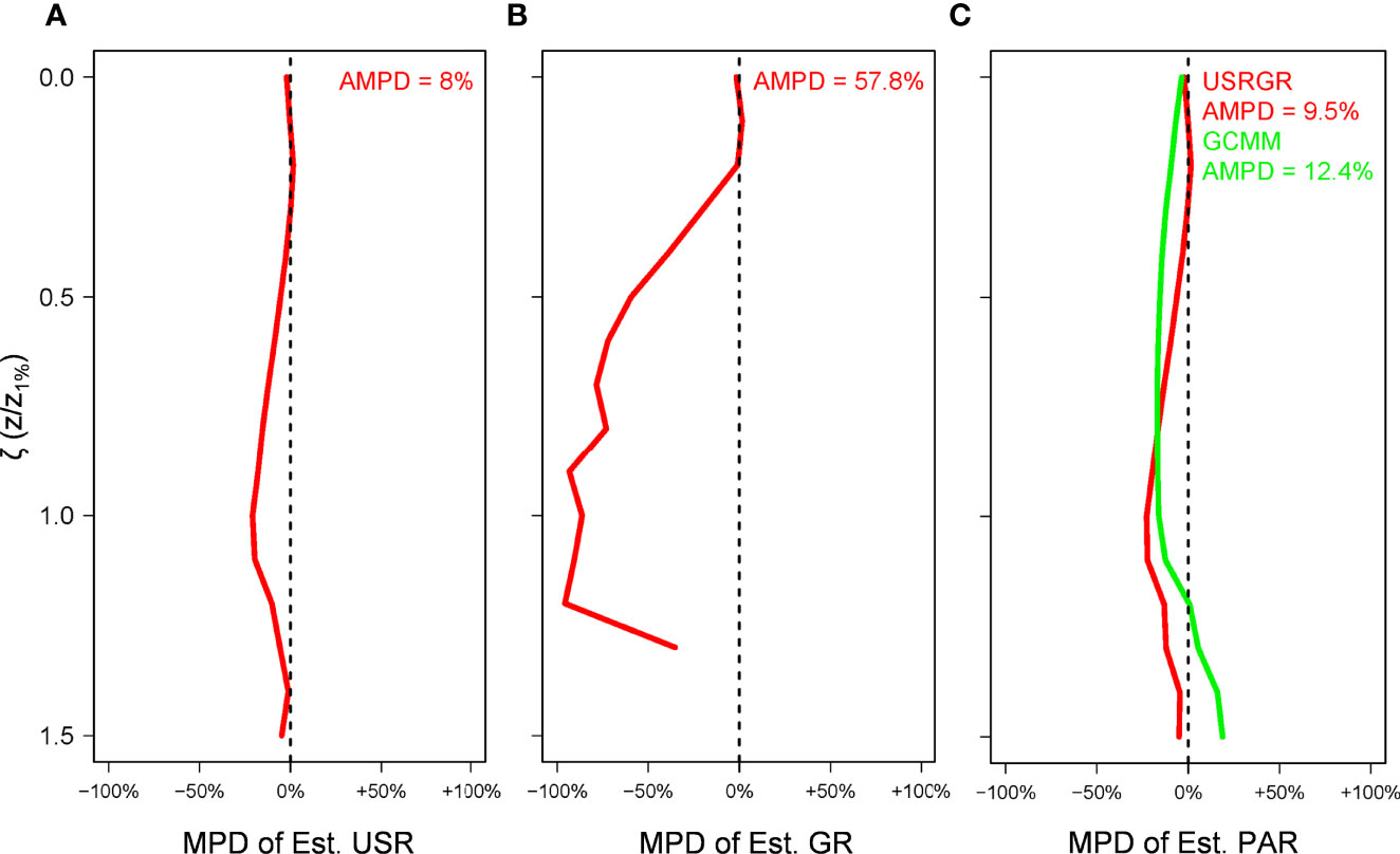
Figure 4 Validation statistics of the estimated USR (A), GR (B), and PAR (C) profiles based on the BIOSOPE cruise dataset. The mean percentage difference (MPD) at each depth was normalized by z1% for the Chl-based USRGR (red) and Chl-based GCMM model (green). The numbers in the legend represent the averaged absolute MPD (AMPD) from the surface to the 1.5-fold z1%.
Besides, the global BGC-Argo dataset compiled by Xing and Boss (2021) was also used here to evaluate the USRGR model in estimating the PAR profile. Here we compared its performance with the Chl-profile-based GCMM model and IOP-based Lee05 model (Lee et al., 2005). The results are shown in Figure 5. For a better evaluation, we characterized all the BGC-Argo Chl profiles into two types, the Mixed Type (maximal Chl locates within the mixed layer) and the DCM Type (maximal Chl locates below the mixed layer). Note that such a classification is only used for the evaluation here and is not required in the general application of the USRGR model. Within the 1.5-fold z1% layer, the USRGR model worked well for both types, with AMPD of 12.5% in Mixed-Type and 9.3% in DCM-Type waters, similar to the performance of GCMM. As discussed in Xing and Boss (2021), Surface-IOP-based Lee05 performed well in the Mixed-Type waters but overestimated the PAR profile in the DCM-Type ones from 0.5-fold to 1.5-fold z1%, reflecting the strong impact of DCM in regulating the attenuation of PAR in the water column.
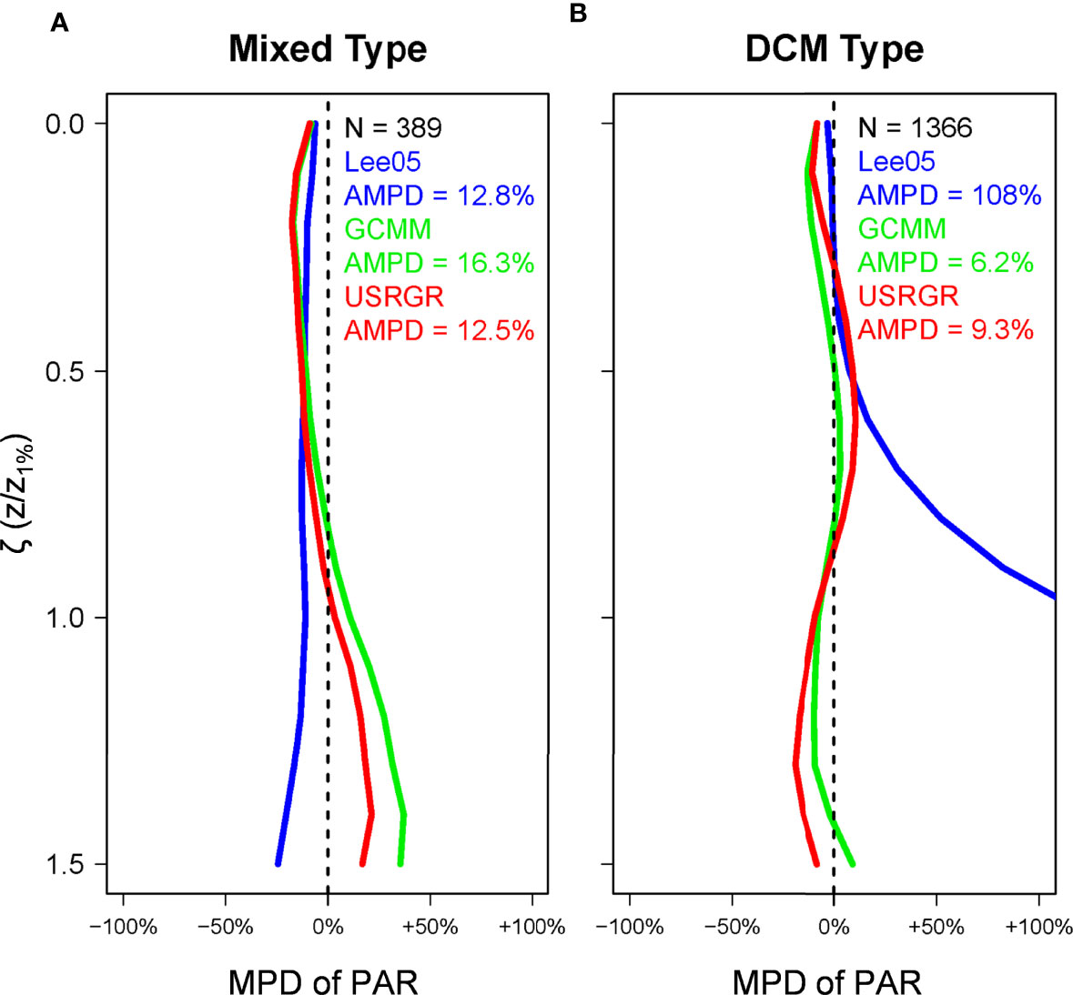
Figure 5 Validation statistics of the estimated PAR profiles based on the global BGC-Argo dataset. The mean percentage difference (MPD) at each depth was normalized by z1% for the estimated PAR by the satellite IOP-based Lee05 (blue), Chl-based USRGR (red), and Chl-based GCMM model (green), for Mixed-Type (maximal Chl locates within the mixed layer) (A) and DCM-Type (maximal Chl locates below the mixed layer) (B) waters, respectively. The numbers in the legend represent the averaged absolute MPD (AMPD) from the surface to the 1.5-fold z1%.
In addition, the USRGR model consumes much shorter computing time than GCMM. A test was conducted to derive the PAR profiles from the global climatological Chl profile data in January; the USRGR model took only 260 s, significantly faster than the GCMM (4195 s) by 93.8%. This is because GCMM decomposes the visible light into 300 wavebands, but USRGR has only two; GCMM frequently calls the GC90 model function, but USRGR only accesses a look-up table of β (Eq. 1).
Estimate of Euphotic Layer Depth From the Chl Profile
It is very common that only Chl observation is available on some in situ observation platforms (e.g., BGC-Argo, glider, as well as the research vehicles) but without radiometry. For example, 53% of the present alive BGC-Argo floats are equipped with Chl fluorometers, but only about 15% with radiometers. The USRGR model, therefore, could be employed to estimate the euphotic layer depth directly from in situ observed Chl profiles; e.g., Xing et al. (2021) estimated z1% based on the GCMM model using BGC-Argo-observed Chl.
Here we adopted the conventional definition of 1% surface PAR (z1%) to represent the euphotic layer depth, although a depth of 0.5% of surface PAR better matches the compensation depth of phytoplankton photosynthesis (Wu et al., 2021). To evaluate the performance of the USRGR model in estimating z1%, the BIOSOPE cruise data were employed (Figure 6). The radiometer-observed z1% showed a wide range from 26 m (in the eutrophic upwelling zone) to 163 m (in the ultra-oligotrophic waters). The USRGR model had a good estimate of z1% with an RMSD of 7.9 m and a little system bias (MPD = -1.5%). In contrast, the surface-Chl-based empirical model of Morel et al. (2007) displayed higher errors (RMSD = 12.9 m), particularly with an obvious underestimation in the ultra-oligotrophic waters (z1% > 140 m), as reported in Xing et al. (2020). In addition, we found that the USRGR model also showed good performance for z0.5%, with RMSD of 7.6 m and MPD of 0% (figure not shown here). It should be noted, similarly, that the USRGR model also admits to estimate euphotic layer depths by other definitions: e.g., z0.1% and z0.9%USR (the depth where USR decreases to 0.9% of sea-surface USR; Wu et al., 2021).
To demonstrate its application, here we applied the USRGR model to the global Chl profile data (Sauzède et al., 2021) to estimate monthly climatological z1%, with the results of January and July shown in Figures 7A and B. Spatially, z1% was deeper in the subtropical gyres and shallower at high latitudes (Southern Ocean and North Atlantic Subpolar region), in the upwelling zones, as well as the summer Oyashio Extension. In the five oligotrophic subtropical gyres, z1% was deeper than 100 m, and the deepest values were found in the Southeast Pacific subtropical gyre (>170 m in summer), consistent with the BIOSOPE data (shown in Figure 6). Moreover, the derived z1% values in other oligotrophic gyres were also in good agreement with previous in situ observations, e.g., with the deepest value of ~140 m in both North and South Atlantic gyres as reported by Poulton et al. (2017) and ~120 m in the Northeast Pacific gyre as recorded by Letelier et al. (2004). On the seasonal scale (comparing Figures 7A, B), for all the five subtropical gyres, z1% was deeper in summer (January in the Southern Hemisphere and July in the Northern Hemisphere) than in winter (July in the Southern Hemisphere and January in the Northern Hemisphere), due to less sea-surface Chl and deeper DCM in summer (Letelier et al., 2004; Mignot et al., 2014). In contrast, z1% at mid-latitudes (30°–60°) was deeper in winter than in summer, due to the characteristics of seasonal stratification, i.e., deep mixing in winter and strong stratification in summer (Xing et al., 2021). The deep mixing in winter eroded DCM and brought some subsurface particles into the mixed layer; such a particle-entrainment process enhanced sea surface Chl, and therefore shoaled z1%; in contrast, the strong stratification in summer obstructed nutrient supply into the mixed layer, and thus the lower Chl at the sea surface and deeper DCM co-determined z1% to be deeper (Xing et al., 2021). Figures 7C, D shows the difference between USRGR-derived z1% and Morel07-derived ones based on MODIS Aqua monthly climatological Chl. Most of the disparity were in subtropical gyres, where USRGR showed deeper z1% than Morel07 in both January and July by 10–40 m (with a maximum relative difference larger than 50%), and their differences were larger in summer, corresponding to less sea-surface Chl and deeper DCM. Besides, USRGR derived shallower z1% than Morel07 in the Southern Ocean and Tropical Eastern Pacific by 20–30 m.
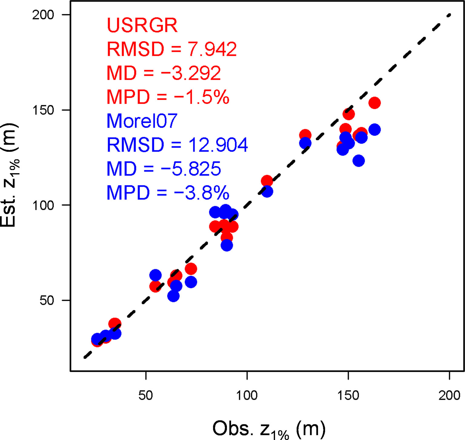
Figure 6 Comparison between the observed and estimated z1% based on the BIOSOPE dataset. Morel07 (blue) represents the surface-Chl-based empirical model proposed by Morel et al. (2007).
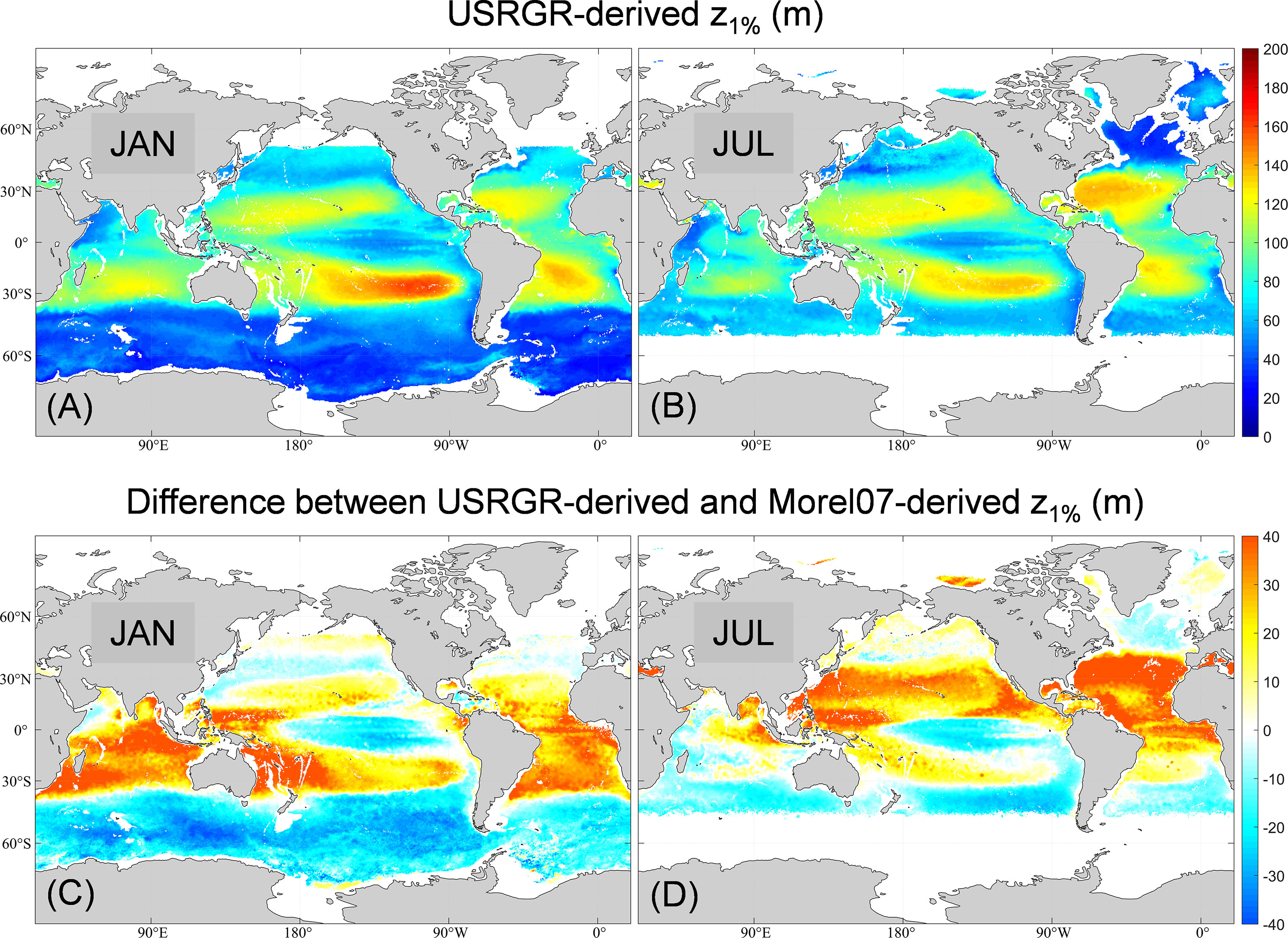
Figure 7 Global monthly climatological z1% in January (A) and July (B), estimated by the USRGR model based on the neural-network-based monthly climatological Chl profile dataset (Sauzède et al., 2021); the difference in z1% between the USRGR model and the Morel07 model (z1% was based on the monthly climatology of MODIS-Aqua Chl) in January (C) and July (D).
Estimate of PAR(0-) for the Underwater PAR Profile
Third, the USRGR model can be employed to estimate the PAR just below the sea surface [i.e., PAR(0-)] from the underwater PAR profile. As mentioned in Section 2.2, the estimation of PAR(0-) generally relies on upward extrapolation from underwater downwelling radiometry. For downwelling irradiance (Ed(λ,z)) at a certain wavelength, the extrapolation based on a linear regression between ln(Ed) and depth is usually adequate with the assumption of vertically uniform IOPs and Kd(λ) within the surface mixed layer. However, this assumption is not valid for downwelling PAR, where Kd(PAR) may vary threefold (much higher Kd(PAR) near the surface for oceanic waters) within the surface 10-m layer (Lee, 2009). Xing et al. (2020) tried to solve the problem by developing a second-degree polynomial function regression between observed ln(PAR) and z, from which PAR(0-) could be estimated through an extrapolation of the regressed equation to z = 0. However, such a regression method is purely empirical. Different from the regression method, here the optimization analysis of the USRGR model (See Applications of the USRGR Model) is based on the bio-optical relationships, despite some empirical equations used. Figure 8 shows the comparison between observed PAR(0-) from the BIOSOPE cruise data and the estimated ones from the USRGR model. All the PAR(0-) were measured around local noon, with a dynamic variation range from 402 μmol photons m-2 s-1 (overcast) to 2,178 μmol photons m-2 s-1 (clear sky). Clearly, the USRGR achieved more accurate estimates than the regression method, with an RMSD of 189 μmol photons m-2 s-1 and a slight bias (MPD = 7.5%).
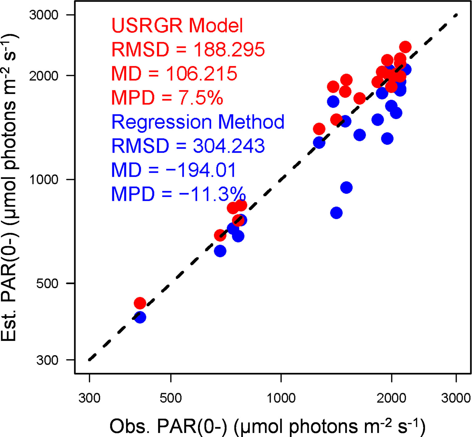
Figure 8 Comparison between the observed and estimated PAR(0-) based on the BIOSOPE dataset. The regression method (blue) represents the regression of second-degree polynomial function (Xing et al., 2020).
Error Source Analysis
The main error sources of the USRGR model stem from three empirical equations (Eqs. 2, 3, and 6), particularly the Chl-Kd(490) bio-optical relationship (Eq. 3). This relationship was established by Morel and Maritorena (2001) based on a global near-surface observation dataset with Chl varying from 0.02 mg m-3 (ultra-oligotrophic) to 40 mg m-3 (eutrophic). However, it is well known that Kd mainly represents the total absorption coefficient (Gordon, 1989; Lee et al., 2005), including the contributions not only from phytoplankton and pure water (both are considered in Eq. 3) but also from chromophoric dissolved organic matter (CDOM) and detritus (also called non-algal particles), which are to some degree correlated with Chl in the open oceans (Bricaud et al., 1998; Morel, 2009). Therefore, the empirical Chl–Kd relationship represents a global near-surface “mean state” of co-varying relationship between phytoplankton and other organic matters. However, the bio-optical anomaly around the mean state exists and some are quite large, particularly for the CDOM–Chl relationship, among different regions (Morel and Gentili, 2009). Besides, as reported by Bricaud et al. (2010), the chlorophyll-specific CDOM generally decreases with depth. That is to say, the near-surface-based Chl–Kd relationship could overestimate deep-water Kd(490) and in turn underestimate USR and PAR to some extent. Therefore, it is not surprising that our BIOSOPE-based analysis results show that the USRGR model slightly underestimated USR and PAR at depth, with the negative maximum of MPD reaching ~-20% (Figures 3 and 4). Since PAR is underestimated to some extent (i.e., PAR is attenuated faster than expected), so is the euphotic layer depth z1% (i.e., shallower than expected) in the ultra-oligotrophic waters, as shown in Figure 6. Nevertheless, the USRGR model still provides a relatively accurate approach to estimate the PAR profile and euphotic layer depth. It is noteworthy that the same error source also exists in the Chl-based GCMM model. At the current stage, there is neither parameterization method nor empirical equation available to correct the CDOM (and/or detritus, suspended particles) anomaly in deep waters; therefore, the USRGR model could be further improved once the contributions from other constituents are better quantified/parameterized in the future.
In addition to the error from the empirical Chl–Kd relationship, the Chl observation/estimation error is also noteworthy. For example, on autonomous mobile platforms (e.g., BGC-Argo, gliders), Chl is estimated by in vivo fluorometers; the Chl-fluorescence variability can introduce additional errors due to the fluorescence efficiency’s uncertainty (Proctor and Roesler, 2010). In some cases, Chl profiling is not available either spatially or temporally; the use of alternative model-estimated Chl profile products (e.g., Uitz et al., 2006; Sauzède et al., 2021; Chen et al., 2022) would also introduce some errors, mainly from the estimated DCM depth, magnitude, and thickness. As analyzed by Xing and Boss (2021), the use of a model-estimated Chl profile (from Uitz et al. (2006)) showed an obvious improvement in estimating the PAR profile in stratified waters, yet with large errors around the euphotic layer depth (MPD of ∼25% at z1%). Although the SOCA-modeled Chl were well evaluated with the global BGC-Argo Chl dataset and a global HPLC Chl database (Sauzède et al., 2021), the averaged absolute percentage error from the Chl profile was reported to be ~40%. We tested the sensitiveness of the USRGR-derived z1% to the Chl uncertainty using the BIOSOPE cruise data, and it is found that the error of +40% and -40% in the Chl profiles would lead to an MPD of 11% and 21% in z1%, respectively (results not shown).
Summary
By decomposing the entire PAR into two wavebands (USR and GR), and then parameterizing their respective attenuation characteristics, here we propose a simplified PAR parameterization model, named USRGR. From a practical point of view, the USRGR model expresses a simple but high-performance approach to model the vertical profiles of PAR for stratified waters. The attenuation of USR maintains the quasi-IOP characteristics, highly related to Kd(490) (Lee et al., 2014; Lin et al., 2016). Taking advantage of the global Chl–Kd empirical relationship (Morel and Maritorena, 2001), the depth-resolved quasi-IOP characteristics can be expressed as a function of the Chl profile. Although some vertical and regional anomalies may affect the accuracy of the Chl–Kd relationship as mentioned in Section 3.4, Chl is still the most common proxy and index of phytoplankton biomass and optical characteristics, in both in situ observations and ecosystem models. Particularly, the fast attenuation of PAR around DCM can be well expressed by the Chl profile, although underestimation may still exist in the estimated PAR profile around z1%. On the other hand, the attenuation of the GR band mainly displays the strong spectral filtering of PAR, with fastest attenuation near the surface and a gradual decrease with depth. Therefore, in this study, the diffuse attenuation coefficient of the GR waveband is parameterized as the function of depth (z) and sea-surface Kd(490).
The new USRGR model is a simplified version of the hyperspectral GCMM model, following the same processing approach: spectral decomposition and vertical IOP variability. Based on the validation results and analyses using the BIOSOPE cruise data and global BGC-Argo dataset, it is well demonstrated that the USRGR model could effectively estimate the PAR profile in both stratified and mixed waters, particularly with a satisfactory performance the same as GCMM in stratified waters. Besides, USRGR is more much efficient, with much less computing time than GCMM (saving more than 90% of time). Third, USRGR is also widely applicable, not only to the in situ observation but also to the marine ecosystem models for estimating the entire PAR profile and euphotic layer depth.
It is also noteworthy that the USRGR-estimated PAR profile is of significance to studies of marine ecosystem dynamics. For example, the median PAR in the mixed layer derived from the PAR profile represents the light condition of mixed-layer phytoplankton growth, which is a key parameter in the photoacclimation models (Behrenfeld et al., 2005; Behrenfeld et al., 2016); z0.415, the isolume depth where the daily PAR value reaches 0.415 mol photons m-2 day-1, is another proxy of compensation depth (Letelier et al., 2004) and can be easily determined from the PAR profile. It has been used in the studies of seasonal algal bloom (e.g., Boss and Behrenfeld, 2010; Cetinić et al., 2015). Recently, some depth-resolved NPP models have been proposed (e.g., Westberry et al., 2008; Fox et al., 2020) for better NPP estimates than the surface-based NPP model (e.g., VGPM); the daily PAR profile, therefore, becomes indispensable in calculating the depth-resolved and vertically-integrated NPP. Especially the neural network model SOCA2021 (Sauzède et al., 2021) provides not only the monthly climatological Chl and backscattering profiles [a proxy for phytoplankton carbon (Graff et al., 2015)] but also the 22-year consecutive weekly Chl and backscattering profiles (1998–2019). The global weekly depth-resolved NPP can be well determined based on the PAR profile estimated from the USRGR model.
Data Availability Statement
The original contributions presented in the study are included in the article/Supplementary Material. Further inquiries can be directed to the corresponding author.
Author Contributions
ZL designed the concept. PX and FC coordinated the overall research project. SC contributed to the remote sensing data analysis. XX was responsible for data processing and drafting the manuscript. All authors revised the manuscript. All authors contributed to the article and approved the submitted version.
Funding
This work is supported by the National Natural Science Foundation of China (41890805, 41876032).
Conflict of Interest
The authors declare that the research was conducted in the absence of any commercial or financial relationships that could be construed as a potential conflict of interest.
Publisher’s Note
All claims expressed in this article are solely those of the authors and do not necessarily represent those of their affiliated organizations, or those of the publisher, the editors and the reviewers. Any product that may be evaluated in this article, or claim that may be made by its manufacturer, is not guaranteed or endorsed by the publisher.
Acknowledgments
The authors are grateful to Prof. Hervé Claustre (Laboratoire d’Océanographie de Villefranche, Sorbonne Université, Villefranche-sur-Mer, France) for providing the BIOSOPE cruise data, the Copernicus Marine Environment Monitoring Service (CMEMS) for distributing the monthly climatological Chl profile data, and all the BGC-Argo data providers and the principal investigators of related BGC-Argo float missions and projects. The BGC-Argo data were collected and made freely available by the International Argo Program (https://doi.org/10.17882/42182), and the BGC-Argo data processing and quality control in this study was conducted in the China Argo Real-time Data Center (http://www.argo.org.cn).
Supplementary Material
The Supplementary Material for this article can be found online at: https://www.frontiersin.org/articles/10.3389/fmars.2022.928807/full#supplementary-material
Footnotes
- ^ https://github.com/BGC-Argo/USRGR/blob/main/Beta1.txt
- ^ https://github.com/BGC-Argo/USRGR/blob/main/USRGREstPARProfile.m
References
Aumont O., Ethé C., Tagliabue A., Bopp L., Gehlen M. (2015). PISCES-V2: An Ocean Biogeochemical Model for Carbon and Ecosystem Studies. Geoscientific Model. Dev. 8 (8), 2465–2513. doi: 10.5194/gmd-8-2465-2015
Behrenfeld M. J. (2010). Abandoning Sverdrup’s Critical Depth Hypothesis on Phytoplankton Blooms. Ecology 91 (4), 977–989. doi: 10.1890/09-1207.1
Behrenfeld M. J., Boss E., Siegel D. A., Shea D. M. (2005). Carbon-Based Ocean Productivity and Phytoplankton Physiology From Space. Global Biogeochemical Cycles 19, GB1006. doi: 10.1029/2004gb002299
Behrenfeld M. J., O’Malley R. T., Boss E. S., Westberry T. K., Graff J. R., Halsey K. H., et al. (2016). Revaluating Ocean Warming Impacts on Global Phytoplankton. Nat. Climate Change 6, 323–330. doi: 10.1038/nclimate2838
Boss E., Behrenfeld M. (2010). In Situ Evaluation of the Initiation of the North Atlantic Phytoplankton Bloom. Geophysical Res. Lett. 37, L18603. doi: 10.1029/2010GL044174
Bricaud A., Babin M., Claustre H., Ras J., Tièche F. (2010). Light Absorption Properties and Absorption Budget of Southeast Pacific Waters. J. Geophysical Research: Oceans 115, C08009. doi: 10.1029/2009JC005517
Bricaud A., Morel A., Babin M., Allali K., Claustre H. (1998). Variations of Light Absorption by Suspended Particles With the Chlorophyll a Concentration in Oceanic (Case 1) Waters: Analysis and Implications for Bio-Optical Models. J. Geophysical Res. 103, 31033–31044. doi: 10.1029/98JC02712
Bryant J. A., Aylward F. O., Eppley J. M., Karl D. M., Church M. J., DeLong E. F. (2016). Wind and Sunlight Shape Microbial Diversity in Surface Waters of the North Pacific Subtropical Gyre. ISME 10, 1308–1322. doi: 10.1038/ismej.2015.221
Buesseler K. O., Boyd P. W., Black E. E., Siegel D. A. (2020). Metrics That Matter for Assessing the Ocean Biological Carbon Pump. Proc. Natl. Acad. Sci. 117 (18), 9679–9687. doi: 10.1073/pnas.1918114117
Byun D.-S., Wang X. H., Hart D. E., Zavatarelli M. (2014). Review of PAR Parameterizations in Ocean Ecosystem Models. Estuarine Coast. Shelf Sci. 151, 318–323. doi: 10.1016/j.ecss.2014.05.006
Carder K. L., Chen R., Hawes S. K. (2003). Instantaneous Photosynthetically Available Radiation and Absorbed Radiation by Phytoplankton, MODIS Ocean Science Team Algorithm Theoretical Basis Document, ATBD MOD-20, Version 7 (Greenbelt, Md: NASA Goddard Space Flight Cent.), 24 pp. Available at: http://modis.gsfc.nasa.gov/data/atbd/atbd_mod20.pdf.
Carlson C., Ducklow H., Michaels A. (1994). Annual Flux of Dissolved Organic Carbon From the Euphotic Zone in the Northwestern Sargasso Sea. Nature 371, 405–408. doi: 10.1038/371405a0
Cetinić I., Perry M. J., D’Asaro E., Briggs N., Poulton N., Sieracki M. E., et al. (2015). A Simple Optical Index Shows Spatial and Temporal Heterogeneity in Phytoplankton Community Composition During the 2008 North Atlantic Bloom Experiment. Biogeosciences 12, 2179–2194. doi: 10.5194/bg-12-2179-2015
Chai F., Dugdale R. C., Peng T. H., Wilkerson F. P., Barber R. T. (2002). One Dimensional Ecosystem Model of the Equatorial Pacific Upwelling System. 1. Model Development and Silicon and Nitrogen Cycle. Deep Sea Res. Part II 49, 2713–2745. doi: 10.1016/S0967-0645(02)00055-3
Chen J., Gong X., Guo X., Xing X., Lu K., Gao H., et al. (2022). Improved Perceptron of Subsurface Chlorophyll Maxima by a Deep Neural Network: A Case Study With BGC-Argo Float Data in the Northwestern Pacific Ocean. Remote Sens. 14, 632. doi: 10.3390/rs14030632
Claustre H., Sciandra A., Vaulot D. (2008). Introduction to the Special Section: Bio-Optical and Biogeochemical Conditions in the South East Pacific in Late 2004—The BIOSOPE Program. Biogeosciences 5, 679–691. doi: 10.5194/bg-5-679-2008
Evans G. T., Parslow J. S. (1985). A Model of Annual Plankton Cycles. Biol. Oceanogr. 24, 483–494. doi: 10.1080/01965581.1985.10749478
Fasham M. J. R., Holligan P. M., Pugh P. R. (1983). The Spatial and Temporal Development of the Spring Phytoplankton Bloom in the Celtic Sea, April 1979. Prog. Oceanogr. 12, 87–145. doi: 10.1016/0079-6611(83)90007-1
Fennel K., Wilkin J., Levin J., Moisan J., O’Reilly J., Haidvogel D. (2006). Nitrogen Cycling in the Middle Atlantic Bight: Results From a Three-Dimensional Model and Implications for the North Atlantic Nitrogen Budget. Global Biogeochemical Cycles 20, GB3007. doi: 10.1029/2005GB002456
Fox J., Behrenfeld M. J., Haëntjens N., Chase A., Kramer S. J., Boss E., et al. (2020). Phytoplankton Growth and Productivity in the Western North Atlantic: Observations of Regional Variability From the NAAMES Field Campaigns. Front. Mar. Sci. 7,24. doi: 10.3389/fmars.2020.00024
Fujii M., Boss E., Chai F. (2007). The Value of Adding Optics to Ecosystem Models: A Case Study. Biogeosciences 4, 817–835. doi: 10.5194/bg-4-817-2007
Gnanadesikan A., Anderson W. G. (2009). Ocean Water Clarity and the Ocean General Circulation in a Coupled Climate Model. J. Phys. Oceanogr. 39, 314–332. doi: 10.1175/2008JPO3935.1
Gordon H. R. (1989). Can the Lambert-Beer Law be Applied to the Diffuse Attenuation Coefficient of Ocean Water? Limnol. Oceanogr. 34, 1389–1409. doi: 10.4319/lo.1989.34.8.1389
Graff J. R., Westberry T. K., Milligan A. J., Brown M. B., Dall’Olmo G., Van Dongen-Vogels V., et al. (2015). Analytical Phytoplankton Carbon Measurements Spanning Diverse Ecosystems. Deep Sea Res. Part I 102, 16–25. doi: 10.1016/j.dsr.2015.04.006
Gregg W. W., Carder K. L. (1990). A Simple Spectral Solar Irradiance Model for Cloudless Maritime Atmospheres. Limnol. Oceanogr. 35 (8), 1657–1675. doi: 10.4319/lo.1990.35.8.1657
Guinehut S., Dhomps A.-L., Larnicol G., Le Traon P.-Y. (2012). High Resolution 3D Temperature and Salinity Fields Derived From in Situ and Satellite Observations. Ocean Sci. 8 (5), 845–857. doi: 10.5194/os-8-845-2012
Lee Z. (2009). KPAR: An Optical Property Associated With Ambiguous Values. J. Lake Sci. 21, 159–164. doi: 10.18307/2009.0202
Lee Z. P., Carder K. L., Marra J., Steward R. G., Perry M. J. (1996). Estimating Primary Production at Depth From Remote Sensing. Appl. Optics 35, 463–474. doi: 10.1364/AO.35.000463
Lee Z., Du K., Arnone R., Liew S., Penta B. (2005). Penetration of Solar Radiation in the Upper Ocean: A Numerical Model for Oceanic and Coastal Waters. J. Geophysical Research: Oceans 110, C09019. doi: 10.1029/2004JC002780
Lee Z., Marra J., Perry M. J., Kahru M. (2015). Estimating Oceanic Primary Productivity From Ocean Color Remote Sensing: A Strategic Assessment. J. Mar. Syst. 149, 50–59. doi: 10.1016/j.jmarsys.2014.11.015
Lee Z., Shang S., Du K., Wei J., Arnone R. (2014). Usable Solar Radiation and its Attenuation in the Upper Water Column. J. Geophysical Research: Oceans 119, 1488–1497. doi: 10.1002/2013JC009507
Letelier R. M., Karl D. M., Abbott M. R., Bidigare R. R. (2004). Light Driven Seasonal Patterns of Chlorophyll and Nitrate in the Lower Euphotic Zone of the North Pacific Subtropical Gyre. Limnol. Oceanogr. 49 (2), 508–519. doi: 10.4319/lo.2004.49.2.0508
Lewis M. R., Carr M. E., Feldman G. C., Esais W., McClain C. (1990). Influence of Penetrating Solar Radiation on the Heat Budget of the Equatorial Pacific Ocean. Nature 347, 543–545. doi: 10.1038/347543a0
Liang X., Wu L. (2013). Effects of Solar Penetration on the Annual Cycle of Sea Surface Temperature in the North Pacific. J. Geophysical Research: Oceans 118, 2793–2801. doi: 10.1002/jgrc.20208
Liang X., Wu L. (2015). Effects of Extratropical Solar Penetration on North Atlantic Ocean Circulation and Climate. Chin. J. Oceanol. Limnol. 33, 243–251. doi: 10.1007/s00343-015-3343-3
Lin J., Lee Z., Ondrusek M., Kahru M. (2016). Attenuation Coefficient of Usable Solar Radiation of the Global Oceans. J. Geophysical Research: Oceans 121, 3228–3236. doi: 10.1002/2015JC011528
Liu Y., He R., Lee Z. (2021). Effects of Ocean Optical Properties and Solar Attenuation on the Northwestern Atlantic Ocean Heat Content and Hurricane Intensity. Geophysical Res. Lett. 48, e2021GL094171. doi: 10.1029/2021GL094171
Liu T., Lee Z., Shang S., Xiu P., Chai F., Jiang M. (2020). Impact of Transmission Scheme of Visible Solar Radiation on Temperature and Mixing in the Upper Water Column With Inputs for Transmission Derived From Ocean Color Remote Sensing. J. Geophysical Research: Oceans 125, e2020JC016080. doi: 10.1029/2020JC016080
Lorenzen C. J. (1972). Extinction of Light in the Ocean by Phytoplankton. ICES J. Mar. Sci. 34 (2), 262–267. doi: 10.1093/icesjms/34.2.262
Manizza M., Le Quéré C., Watson A. J., Buitenhuis E. T. (2005). Bio-Optical Feedbacks Among Phytoplankton, Upper Ocean Physics and Sea-Ice in a Global Model. Geophysical Res. Lett. 32, L05603. doi: 10.1029/2004GL020778
Mignot A., Claustre H., Uitz J., Poteau A., D’Ortenzio F., Xing X. (2014). Understanding the Seasonal Dynamics of Phytoplankton Biomass and the Deep Chlorophyll Maximum in Oligotrophic Environments: A Bio-Argo Float Investigation. Global Biogeochemical Cycles 28, 856–876. doi: 10.1002/2013GB004781
Mignot A., Ferrari R., Claustre H. (2018). Floats With Bio-Optical Sensors Reveal What Processes Trigger the North Atlantic Bloom. Nat. Commun. 9 (1), 190. doi: 10.1038/s41467-017-02143-6
Mobley C. D., Boss E. (2012). Improved Irradiances for Use in Ocean Heating, Primary Production, and Photo-Oxidation Calculations. Appl. Optics 51, 6549–6560. doi: 10.1364/ao.51.006549
Morel A. (1988). Optical Modeling of the Upper Ocean in Relation to its Biogenous Matter Content. J. Geophysical Res. 93, 10749–10768. doi: 10.1029/JC093iC09p10749
Morel A. (2009). Are the Empirical Relationships Describing the Bio-Optical Properties of Case 1 Waters Consistent and Internally Compatible? J. Geophysical Research: Ocean 114, C01016. doi: 10.1029/2008JC004803
Morel A., Gentili B. (2009). The Dissolved Yellow Substance and the Shades of Blue in the Mediterranean Sea. Biogeosciences 6, 2625–2636. doi: 10.5194/bg-6-2625-2009
Morel A., Huot Y., Gentili B., Werdell P. J., Hooker S. B., Franz B. A. (2007). Examining the Consistency of Products Derived From Various Ocean Color Sensors in Open Ocean (Case 1) Waters in the Perspective of a Multi-Sensor Approach. Remote Sens. Environ. 111 (1), 69–88. doi: 10.1016/j.rse.2007.03.012
Morel A., Maritorena S. (2001). Bio-Optical Properties of Oceanic Waters: A Reappraisal. J. Geophysical Research: Oceans 106 (C4), 7163–7180. doi: 10.1029/2000JC000319
Organelli E., Claustre H., Bricaud A., Schmechtig C., Poteau A., Xing X. G., et al. (2016). A Novel Near-Real-Time Quality-Control Procedure for Radiometric Profiles Measured by Bio-Argo Floats: Protocols and Performances. J. Atmospheric Oceanic Technol. 33, 937–951. doi: 10.1175/jtech-d-15-0193.1
Paulson C. A., Simpson J. J. (1977). Irradiance Measurements in the Upper Ocean. J. Phys. Oceanogr. 7, 953–956. doi: 10.1175/1520-0485(1977)007<0952:IMITUO>2.0.CO;2
Pimentel S., Tse W.-H., Xu H., Denaxa D., Jansen E., Korres G., et al. (2019). Modeling the Near-Surface Diurnal Cycle of Sea Surface Temperature in the Mediterranean Sea. J. Geophysical Research: Oceans 124, 171–183. doi: 10.1029/2018JC014289
Poulton A. J., Holligan P. M., Charalampopoulou A., Adey T. R. (2017). Coccolithophore Ecology in the Tropical and Subtropical Atlantic Ocean: New Perspectives From the Atlantic Meridional Transect (AMT) Programme. Prog. Oceanogr. 158, 150–170. doi: 10.1016/j.pocean.2017.01.003
Proctor C. W., Roesler C. S. (2010). New Insights on Obtaining Phytoplankton Concentration and Composition From in Situ Multispectral Chlorophyll Fluorescence. Limnol. Oceanogr.: Methods 8, 695–708. doi: 10.4319/lom.2010.8.695
Rochford P. A., Kara A. B., Wallcraft A. J., Arnone R. A. (2001). Importance of Solar Subsurface Heating in Ocean General Circulation Models. J. Geophysical Res. 106 (C12), 30923–30938. doi: 10.1029/2000JC000355Ryther
Ryther J. H. (1956). Photosynthesis in the Ocean as a Function of Light Intensity. Limnol. Oceanogr. 1, 61–70. doi: 10.4319/lo.1956.1.1.0061
Sauzède R., Claustre H., Uitz J., Jamet C., Dall’Olmo G., D’Ortenzio F., et al. (2016). A Neural Network-Based Method for Merging Ocean Color and Argo Data to Extend Surface Bio-Optical Properties to Depth: Retrieval of the Particulate Backscattering Coefficient. J. Geophysical Research: Oceans 121, 2552–2571. doi: 10.1002/2015JC011408
Sauzède R., Renosh P. R., Claustre H. (2021). QUALITY INFORMATION DOCUMENT of Global Ocean 3d Particulate Organic Carbon and Chlorophyll-A Concentration Product MULTIOBS_GLO_BIO_BGC_3d_REP_015_010. doi: 10.48670/moi-00046
Siegel D. A., Buesseler K. O., Doney S. C., Sailley S. F., Behrenfeld M. J., Boyd P. W. (2014). Global Assessment Of Ocean Carbon Export By Combining Satellite Observations And Food-Web Models. Glob. Biogeochem. Cycles 28, 181–196. doi: 10.1002/2013GB004743
Skákala J., Bruggeman J., Brewin R. J. W., Ford D. A., Ciavatta S. (2020). Improved Representation of Underwater Light Field and its Impact on Ecosystem Dynamics: A Study in the North Sea. J. Geophysical Research: Oceans 125, e2020JC016122. doi: 10.1029/2020JC016122
Uitz J., Claustre H., Morel A., Hooker S. B. (2006). Vertical Distribution of Phytoplankton Communities in Open Ocean: An Assessment Based on Surface Chlorophyll. J. Geophysical Res. 111, C08005. doi: 10.1029/2005jc003207
Westberry T., Behrenfeld M. J., Siegel D. A., Boss E. (2008). Carbon-Based Primary Productivity Modeling With Vertically Resolved Photoacclimation. Global Biogeochemical Cycles 22, GB2024. doi: 10.1029/2007gb003078
Wollschläger J., Tietjen B., Voß D., Zielinski O. (2020). An Empirically Derived Trimodal Parameterization of Underwater Light in Complex Coastal Waters – A Case Study in the North Sea. Front. Mar. Sci. 7,512. doi: 10.3389/fmars.2020.00512
Wu J., Lee Z., Xie Y., Goes J., Shang S., Marra J. F., et al. (2021). Reconciling Between Optical and Biological Determinants of the Euphotic Zone Depth. J. Geophysical Research: Oceans 126, e2020JC016874. doi: 10.1029/2020JC016874
Xing X., Boss E. (2021). Chlorophyll-Based Model to Estimate Underwater Photosynthetically Available Radiation for Modeling, in-Situ, and Remote-Sensing Applications. Geophysical Res. Lett. 48, e2020GL092189. doi: 10.1029/2020GL092189
Xing X., Boss E., Chen S., Chai F. (2021). Seasonal and Daily-Scale Photoacclimation Modulating the Phytoplankton Chlorophyll-Carbon Coupling Relationship in the Mid-Latitude Northwest Pacific. J. Geophysical Research: Oceans 126, e2021JC017717. doi: 10.1029/2021JC017717
Xing X., Boss E., Zhang J., Chai F. (2020). Evaluation of Ocean Color Remote Sensing Algorithms for Diffuse Attenuation Coefficients and Optical Depths With Data Collected on BGC-Argo Floats. Remote Sens. 12, 2367. doi: 10.3390/rs1215236
Zaneveld J. R. V., Spinrad R. W. (1980). An Arc Tangent Model of Irradiance in the Sea. J. Geophysical Res. 85 (C9), 4919–4922. doi: 10.1029/JC085iC09p04919
Keywords: photosynthetically available radiation (PAR), usable solar radiation (USR), attenuation model, chlorophyll, euphotic layer depth
Citation: Xing X, Lee Z, Xiu P, Chen S and Chai F (2022) A Dual-Band Model for the Vertical Distribution of Photosynthetically Available Radiation (PAR) in Stratified Waters. Front. Mar. Sci. 9:928807. doi: 10.3389/fmars.2022.928807
Received: 26 April 2022; Accepted: 09 June 2022;
Published: 28 July 2022.
Edited by:
Oliver Zielinski, University of Oldenburg, GermanyReviewed by:
Jochen Wollschläger, University of Oldenburg, GermanyRene Friedland, Leibniz Institute for Baltic Sea Research (LG), Germany
Copyright © 2022 Xing, Lee, Xiu, Chen and Chai. This is an open-access article distributed under the terms of the Creative Commons Attribution License (CC BY). The use, distribution or reproduction in other forums is permitted, provided the original author(s) and the copyright owner(s) are credited and that the original publication in this journal is cited, in accordance with accepted academic practice. No use, distribution or reproduction is permitted which does not comply with these terms.
*Correspondence: Xiaogang Xing, eGluZ0BzaW8ub3JnLmNu