 Rui Tang
 Yi Yu
Yi Yu Jingyuan Xi
 Wentao Ma
 Yuntao Wang
- 1State Key Laboratory of Satellite Ocean Environment Dynamics, Second Institute of Oceanography, Ministry of Natural Resources, Hangzhou, China
- 2Southern Marine Science and Engineering Guangdong Laboratory (Zhuhai), Zhuhai, China
The Kuroshio Extension (KE) region is one of the most energetic regions in the global ocean where prominent mesoscale dynamics persistently occur. The spatial distribution and temporal evolution of the sea surface temperature (SST) gradient and mesoscale eddies in the KE are investigated. The SST gradient can be applied for identifying the fronts, and the SST gradient within two times the radii of the eddies is composited to quantify the impact of eddies on frontal activities. Depressed SST gradients are identified for eddies with both polarities, but prominent spatial variance in the SST gradient reveals that a large SST gradient is located to the north of anticyclones and along the south periphery for cyclones. The eddies are further separated into two groups depending on their location relative to the main path of the KE, as the background fields to the north and south of the KE are largely different. The spatial pattern, e.g., monopole and dipole features, and temporal variation in the SST gradient are fully studied over the lifespans of eddies. The results show that most eddies can significantly weaken the internal SST gradient and induce the horizontal redistribution of the SST gradient in surrounding regions. Cyclonic eddies north of the KE elevate the fronts along the periphery of eddies. The temporal variability in the SST gradient is prominent and largely varies for each group of eddies. This study offers quantitative analyses of the spatial and temporal relationships between eddies and fronts that are important for understanding the mesoscale dynamics in the world’s oceans.
Introduction
The Kuroshio Current, as the western boundary current of subtropical circulation in the North Pacific Ocean, flows northward along the continental margin and is associated with the substantial transport of heat meridionally (Qiu, 2002). To the north of the Kuroshio Current, there is another western boundary current of subarctic circulation, namely, the Oyashio Current, characterized as cold and nutrient-rich, which flows southward and merges with the Kuroshio Current (Tatebe and Yasuda, 2004). The confluence of the Kuroshio Current and Oyashio Current takes place and then turns eastward into the open ocean, which is referred to as the Kuroshio Extension (KE) (Itoh and Yasuda, 2010). There are abundant mesoscale activities in the KE region, e.g., fronts and eddies, owing to the large instability established as these two distinctive currents converge (Mizuno and White, 1983; Yasuda, 2003; Itoh and Yasuda, 2010; Kida et al., 2015), and two quasi-stationary meanders with ridges are located at 144°E and 151°E, indicating the instabilities of currents (Qiu, 2002). These processes have a significant impact on the energy budget, air-sea interactions, and fisheries (Sugimoto and Tameishi, 1992; Kida et al., 2015; Shan et al., 2020). Therefore, the KE region has drawn much attention due to the complex dynamic processes.
Eddies, as the major category of mesoscale dynamics (Chai et al., 2020), have a spatial scale where the radius ranges from 25-250 km and the lifespan is longer than 10 days (Chelton et al., 2011b). The majority of eddies are characterized by a westward propagating tendency, similar to Rossby waves (Chelton et al., 2007), leading to a gentle sea surface height (SSH) gradient of the leading edge and a steepened SSH gradient of the trailing edge (Early et al., 2011). As a result, the geostrophic current induced by eddies is stronger at the eastern side than at the western side, which makes the anticyclonic (cyclonic) eddies have a slightly equatorward (poleward) propagation tendency (Chelton et al., 2007). Eddies have important influences on water properties, e.g., temperature, salinity and chlorophyll-a, in both the horizontal and vertical directions (Nurser and Zhang, 2000; Itoh and Yasuda, 2010; Early et al., 2011; Frenger et al., 2015) via several dynamical processes, including eddy trapping, eddy pumping, eddy stirring, etc. (Gaube et al., 2014). For example, there are often positive (negative) SST anomalies and elevated (reduced) wind stress aloft inside anticyclonic (cyclonic) eddies, which is due to the downwelling (upwelling) induced by eddy pumping (Ma et al., 2015).
The response caused by the above dynamic mechanisms can be divided into monopoles and dipoles according to the characteristics of the responses (Siegel et al., 2011). Eddy trapping caused by eddy nonlinear characteristics means that the rotational speed of eddies is larger than the velocity of the background field (Chelton et al., 2007). Through this dynamic mechanism, eddies can carry water masses from the background origin over a long period of time and remain sealed (Chelton et al., 2011a). In the process of eddy formation, eddy pumping induced by the convergence/divergence of sea surface water can induce upwelling (downwelling) in cyclonic (anticyclonic) eddies (Benitez-Nelson et al., 2007). These two mechanisms lead to monopole anomalies (Gaube et al., 2014). Based on the rotation of eddies, another dynamic mechanism called eddy advection affects the distribution of water masses in eddies, which stirs the background field and leads to upwelling near the eddy edge (Mizobata et al., 2002; Chelton et al., 2011a) and finally develops a dipole anomaly (Siegel et al., 2011). In general, the anomalies caused by eddies can be considered a combination of these anomalies induced by the above dynamic mechanisms. The importance of each dynamic mechanism varies during the whole lifecycle of eddies; for example, the effect of eddy stirring is larger than that of eddy pumping after eddy generation, but eddy pumping is stronger than eddy stirring before eddies vanish (Gaube et al., 2014).
In the KE region, eddies are mostly generated by horizontal shear instability and KE main path meander instability (Ji et al., 2018). For the first mechanism, the inconsistent horizontal flow rate results in the curl of flow that gradually develops into eddies, which are usually smaller in scale and short-lived. Accordingly, the westward retroflection, derived from the KE, can generate anticyclonic (cyclonic) eddies in the south (north). The second mechanism of eddy generation is caused by the meandering of the main path of the KE, which means that the “meanders” are split away from the KE. The eddies generated by this mechanism can be long-lived and have a relatively stable structure. Thus, the anticyclonic (cyclonic) eddies are mostly on the north side (south side) of the main path of the KE, which is contrary to the other mechanism. Because the eddies produced by these two mechanisms have different features, the eddies are not evenly distributed in the KE region. Long-lived anticyclonic (cyclonic) eddies are mainly distributed on the north side (south side) of the KE path, while short-lived eddies are the opposite (Ji et al., 2018).
The eddy-induced responses in oceanic features in both the horizontal and vertical directions are highly complex due to their underlying dynamic processes (Nurser and Zhang, 2000; Wang et al., 2018; Sun et al., 2020). For instance, in the horizontal direction, eddy stirring is the azimuthal advection around eddy peripheries associated with the transport of water properties, while eddy trapping is caused by the nonlinear characteristics of eddies, for which the rotational velocities of the eddy are faster than the eddy propagation speed, leading to inside fluid trapping (McWilliams and Flierl, 1979; Gaube et al., 2014). In the vertical direction, eddy pumping is the vertical motion of the eddy center caused by eddy-induced isopycnal displacement during the intensification of eddies (Gaube et al., 2015). Eddy-induced Ekman pumping is another vertical motion, which is a nonlinear process formed by the interaction between eddies and sea surface wind (Yang et al., 2021). Eddy-induced Ekman pumping is usually characterized by an opposite impact to that of eddy pumping (Gaube et al., 2014).
In addition, there are significant spatial variabilities in local dynamics and ecosystems in the KE region, especially in the meridional direction. For example, the SSH varies prominently and generally decreases poleward (Qiu and Chen, 2011), and the region with the largest meridional sea surface temperature (SST) gradient is used to represent the main path of the KE (Qiu et al., 2014). The spatial variation also varies over time; for instance, the SST has a larger range in the north than in the south of the KE main path, resulting in a larger meridional SST gradient during winter than during other seasons (Sato et al., 2016). Under these conditions, another mesoscale process, referred to as the front, which is defined as a narrow transition zone between water masses by using SST gradients (Kostianoy and Lutjeharms, 1999; Wang et al., 2015), is established (Xi et al., 2022). The SST fronts induced by the confluence of cold and warm water in the KE region are mainly distributed from 35°N to 45°N, e.g., the Kuroshio Extension Front and the Subarctic Boundary Front (Yasuda, 2003; Itoh and Yasuda, 2010; Kida et al., 2015). The intensity of the front, i.e., the SST gradient, over the Subarctic Boundary Front is stronger than that over the Kuroshio Extension Front (Jing et al., 2019). Temporal variability in frontal intensity also varies, and Sato et al. (2016) observed that the SST gradient is weak in summer, although the SST front on the north side of the KE near the coast of eastern Japan is maintained or strengthened in June and July. These SST fronts have an important impact on primary production and fisheries (Rykaczewski et al., 2015). Wang et al. (2021b) found a positive spatial-temporal correlation between the SST gradient and chlorophyll-a concentrations (Chl-a) in the KE region after investigating the variability in the SST gradient and Chl-a and indicated that the SST gradient can be used to predict the interannual variability in Chl-a.
Most previous studies have mainly focused on the SST anomaly induced by eddy-related dynamical processes (Frenger et al., 2015; Gaube et al., 2015). For example, in the North Pacific, anticyclonic (cyclonic) eddies represent a warm (cold) internal core (Hausmann and Czaja, 2012; Sun et al., 2020). Regarding the SST gradient, which is used as a proxy for fronts (Xi et al., 2022), few studies have investigated the influence of eddies on modulating the SST gradient. For instance, Wang et al. (2020) revealed that eddies in the KE region can carry the front as they move westward and that the front gradually weakens. The eddies can expand the region with a large SST gradient in the preexisting frontal zone (Yuan and Castelao, 2017). However, an understanding of the effects of eddies on SST gradients and of the spatial variability in SST gradients induced by eddies is still lacking. In this study, we used a dataset of mesoscale eddies and long-term satellite observations of SST gradients to analyze the influence of eddies on SST gradients in the KE region. The data and method are described in section 2. The results are summarized in section 3. The discussion and the conclusions are presented in sections 4 and 5, respectively.
Data and method
Satellite observations of SST are used to obtain the SST gradient in the study region (140°E-170°E, 30°N-40°N). The daily SST data are measured by the Moderate Resolution Imaging Spectroradiometer (MODIS), which is onboard the Aqua satellite. The spatial resolution of SST data is 1/24°, which is approximately 4.5 km, and the time spans from July 2002 to the present. SST gradients have been widely used to describe frontal activities in the global oceans. SST gradients are calculated at each pixel for their zonal component (Gx) and meridional component (Gy) as the ratio of the SST difference among the surrounding pixels following Wang et al. (2021b). The total gradient (G) is subsequently calculated as .
The applied SSH data, with a spatial resolution of 1/4° covering the period from July 2002 to December 2015, are obtained from the Copernicus Marine Environment Monitoring Service (CMEMS). The daily KE main path is defined by the SSH contour with a constant value following Qiu et al. (2014). In a former study, the contour of 100 centimeters is applied to depict the main path of KE, but a value of 170 centimeters is used with the SSH data here. The difference in SSH data between CMEMS and the one used in Qiu et al. (2014) is assessed, and the identified KE main paths are mostly identical between both studies.
The mesoscale eddies are identified with satellite altimeter data, which are acquired from Archiving, Validation and Interpretation of Satellite Oceanographic (AVISO) data, which is released by Chelton et al. (2011b) with the location, radius, date, and amplitude information for each eddy’s trajectory. The dataset is also provided by the CMEMS, and the spatial resolution and temporal period are the same as those of the SSH data. Note that the eddy can exist or be distinct without being included in the dataset because its amplitude is too small to be detected in the altimeter data. The life cycle for each eddy is calculated using the entire identified trajectory as the existing period divided by the total length of the lifetime. This dataset has been widely used in the global ocean, and the identified eddy feature is highly representative of the KE region (Meng et al., 2021). The spatial distribution of eddies in the KE region is described with the frequency of eddy occurrence, which is calculated at each pixel as the counted number of days that it was inside an eddy divided by the total number of days, i.e., 4932 days. Although eddies have different shapes, we adopted the feature following Chelton et al. (2011b), where all eddies are defined as circles and their area is equivalent to the identified area of eddies.
To quantitatively investigate the impact of eddies on the distribution of the SST gradient, the composite method is applied. Because of substantial cloud coverage, seven-day averaged SST gradient at daily intervals is applied. The snapshot of the SST gradient within twice of each eddy’s radius is first obtained, and those with more than 50% cloud coverage are eliminated to reduce the cloud impact. Due to the different sizes of eddies, the snapshots are linearly interpolated to be the same size, e.g., a radius of 375 km. In this study, small eddies, which have a radius of less than 65 km, are eliminated since each pixel within small eddies will be interpolated into 6 pixels or more, leading to limited spatial variation for eddy-induced patterns. Finally, all snapshots are composited by calculating their average, and the standard deviation is subsequently obtained. Moreover, the SST gradient anomaly is calculated for each snapshot by removing the spatial average of each corresponding eddy. The eddy-induced SST gradients are separated into monopole and dipole features, where the monopole feature is calculated as the average of the concentric circles over different distances from the eddy center and the dipole feature is the residual of the total SST gradient eddy after removing the monopole feature (He et al., 2019).
Result
Based on daily satellite SST observations, the SST gradient in the KE region shows a large spatial variation (Figure 1A). A strong SST gradient is identified in the KE region, particularly in the northern KE, i.e., the Subarctic Boundary Front, and near the coast of Japan. In comparison, a weaker SST gradient is found to the south of the KE, i.e., the Kuroshio Extension Front (Jing et al., 2019). The meridional difference of the strong and weak SST gradient can be prominently identified along the KE, especially in the region to the west of 155°E. In the region to the east of 155°E, the meridional difference is less prominent and has a weakened SST gradient for the entire region. The region with a strong SST gradient is similar to the formerly identified frontal region, such as the Subarctic Front and the Kuroshio Bifurcation Front (Itoh and Yasuda, 2010), revealing that the SST gradient can be applied as an indicator of fronts.
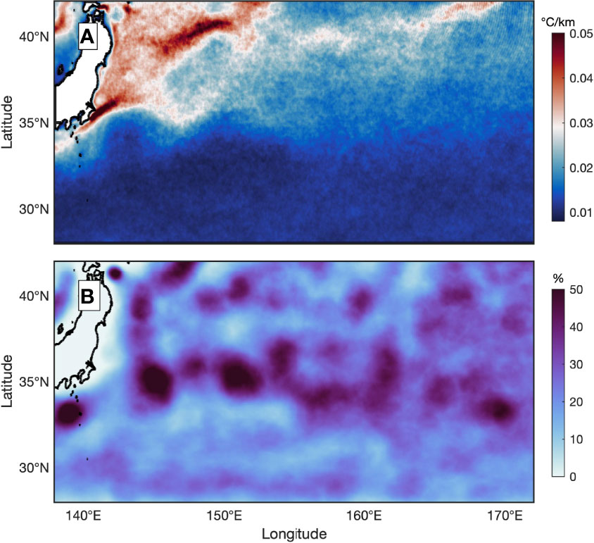
Figure 1 (A) Averaged sea surface temperature (SST) gradient (°C/km) and (B) averaged eddy occurrence (%) in the Kuroshio Extension (KE) region. In (B), the averaged eddy occurrence for each pixel is equal to the number of days the eddy exists divided by the total number of days.
The spatial distribution of eddies (Figure 1B) has a very different pattern than that of the SST gradient. In particular, the difference in eddy occurrence between the north and south sides of the KE is much less obvious than the SST gradient. The region with a high frequency of eddy occurrence is mainly distributed zonally along 35°N, which is consistent with the main path of the KE. The two large meanders of the KE also show a high frequency of eddy occurrence. Thus, the instability of the KE fosters a large number of eddies. Notably, there are almost no eddies between 35° N and 40° N near the coast, but a high eddy occurrence generally occurs in the surrounding areas.
To avoid cloud contamination and bias induced by interpolation, eddies with cloud coverage greater than 50% or those with a radius less than 65 km are eliminated. There are 65,010 snapshots of eddies in total (29,185 anticyclonic eddies and 35,825 cyclonic eddies) for compositing use in the study region. The mean radius and lifetime of anticyclonic eddies are 93.43 km and 136 days, respectively, and those of cyclonic eddies are 87.09 km and 137 days, respectively. The overall SST gradients for anticyclonic and cyclonic eddies are approximately the same, and their values are 18.5×10⁻³°C/km and 18.2×10⁻³°C/km, respectively. For anticyclonic eddies, the SST gradient is largely weakened within the eddy, and the minimum SST gradient reaches 12.3×10⁻³°C/km near the center (Figure 2A). An anticyclonic eddy strengthens the SST gradient on its north side, and the maximum SST gradient appears outside one radius of the eddy, reaching 27.2×10⁻³°C/km. For cyclonic eddies, the SST gradient is generally weak near the center of the eddy and to the north, and a small SST gradient is identified at nearly twice the eddy radius in the south, with a minimum reach of 15.2×10⁻³°C/km (Figure 2B). A band with a strengthened SST gradient appears along the south side of the eddy periphery, where the maximum SST gradient reaches 22.7×10⁻³°C/km. Thus, the anticyclonic eddies are associated with a slightly larger SST gradient, with an inhibited value inside the eddy; cyclonic eddies have an elevated SST gradient in the south periphery, associated with complex spatial variation in the SST gradient.
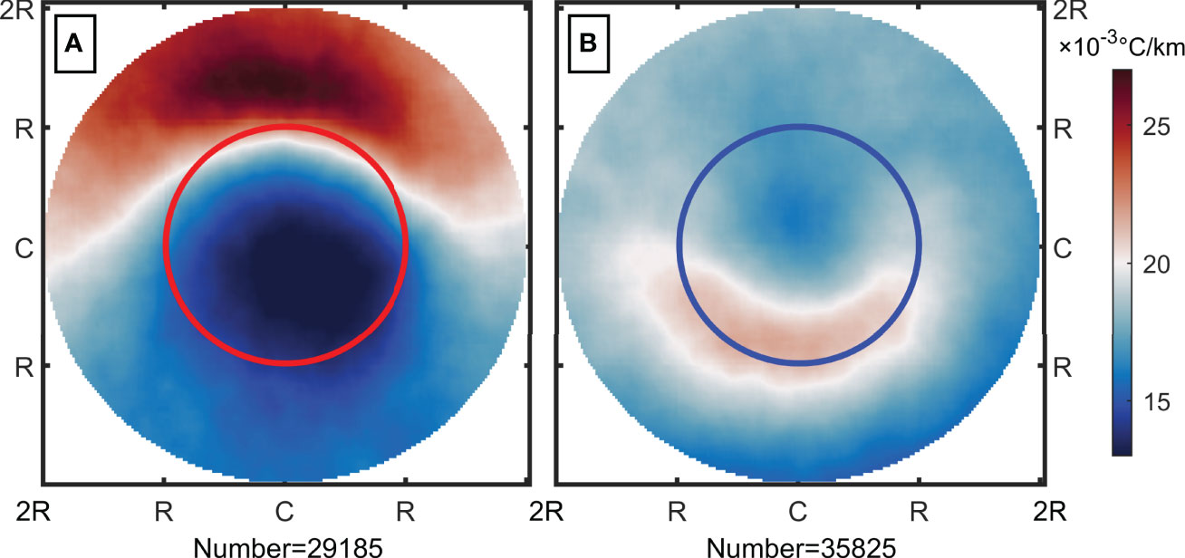
Figure 2 Composite of the SST gradient (×10-3°C/km) for (A) an anticyclone and (B) a cyclone within twice the eddy radius. The red (blue) circle represents the radius of the anticyclonic (cyclone) eddy, and the total number of composite eddies is shown in each panel.
To evaluate the eddy impact to the north and south of the KE main path, the SSH is used to delineate the main path of the KE following Qiu et al. (2014). The daily eddies to the north and south of the KE are subsequently distinguished (Figure 3A), and the overall eddy occurrence percentage is further obtained (Figures 3B, C). Compared with the averaged main path of the KE, obtained as the 170 cm contour of climatologically averaged SSH, the distribution of eddies is well divided. The overall number of eddy occurrences is approximately the same between the north and south, although the number of eddy occurrences does not equally separate in space. For example, two regions with high eddy occurrences along the main path of the KE to the west of 155°E are both present on the south side (Figure 3C). However, the high eddy occurrence east of 155°E is mostly separated into the north side. Note that the eddies located at the boundary of the study region are not included in this study.
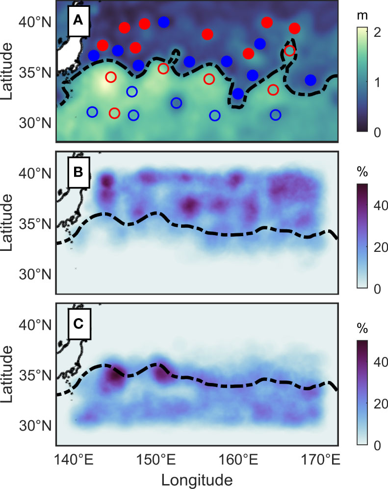
Figure 3 (A) Example of delineating the north and south sides of the KE with daily sea surface height (SSH) on September 26, 2004, and the corresponding eddies on each side. The black dotted line is the 170 cm SSH contour, representing the main path of the KE. Red (blue) circles represent the centers of the anticyclone (cyclone), and solid (hollow) circles represent eddies in the north (south). (B, C) represent the percentages of eddy occurrence to the north and south of the KE main path, overlaid with the averaged main path of KE (dashed line).
Based on the polarities of eddies and their relative locations to the main path of the KE, four groups of eddies are delineated. Their temporal evolution of the averaged SST gradient within two radii of the eddies shows prominent variation over the lifetime of the eddies (Figure 4). For all groups of eddies, the fluctuation in the SST gradient over the lifetime is more than 1×10⁻³°C/km, although the variation over time is different for each group. The SST gradient in the anticyclonic eddies in the north rapidly weakens after generation and rebounds to a larger value than the initial gradient at approximately 0.4 of their lifetimes but weakens quickly and remains at approximately the initial gradient until their termination (Figure 4A). For cyclonic eddies in the north, the SST gradient decreases during the first half of their lifetime and increases during the second half of their lifetime to a value similar to the initial gradient (Figure 4B). The anticyclonic eddy in the south is the only group with an enhanced SST gradient during the first 0.6 of their lifetimes until a sudden weakening and enhancement of approximately 0.65 and 0.84 occur, respectively (Figure 4C). The SST gradient in south cyclonic eddies weakens after eddy generation, with a large strengthening during the middle phase of their lifetime, and returns to normal at the end (Figure 4D). The south eddies have more complex mechanics, where two crests and two troughs are generally identified during their lifetimes, but the SST gradient is larger in the north. Note that eddies are not detected during the time of their generation due to the small sea level anomaly (SLA) (Gaube et al., 2014); thus, the initial SST gradient actually incorporates the impact of eddies after a period of eddy intensification.
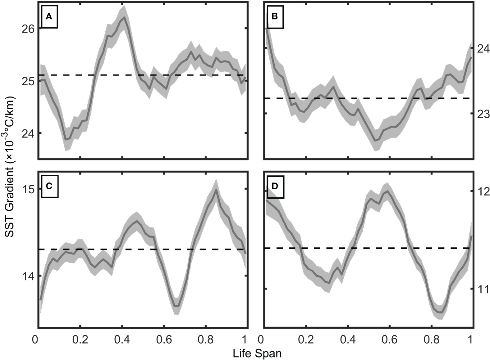
Figure 4 Temporal evolutions of the averaged SST gradient (×10-3°C/km) for (A) an anticyclone and (B) a cyclone in the north and (C) an anticyclone and (D) a cyclone in the south over the lifetimes of the eddies. The dashed horizontal line represents the corresponding overall average. The gray shading represents standard errors.
The SST gradients of eddies in the four groups are further composited to obtain their respective spatial patterns (Figure 5). The background average of the SST gradient for each eddy is removed before composition; thus, the influence of eddies on the SST gradient is revealed in the anomalous field. The eddies with different polarities have a generally consistent pattern with the overall average (Figure 2); the strengthened SST gradient zone is located on the north (south) side of the anticyclonic (cyclonic) eddy, and the value is weakened near the eddy center. The maximum (minimum) SST gradients are 12 (-9)×10-3°C/km, 5.9 (-5) ×10-3°C/km, 6.4 (-4) ×10-3°C/km and 1 (-2) ×10-3°C/km for the anticyclone and cyclone in the north and the anticyclone and cyclone in the south, respectively. Obviously, the eddies on the north side induce larger variations in the SST gradient. A detailed comparison shows that the distribution of the SST gradient in eddies also varies in space. For anticyclonic eddies in the north, a large SST gradient is located slightly outside the north of the periphery, and the range of the SST gradient anomaly is large (Figure 5A). However, for anticyclones in the south, the large SST gradient is located closer to twice the radius in the north, which is associated with a limited range of the SST gradient (Figure 5G). In terms of cyclonic eddies, the SST gradient for eddies in the north is highly consistent with the spatial pattern of the overall average in cyclones (Figures 2B, 5D), but those in the south show large negative values near the center associated with weak positive values outside the periphery (Figure 5J).
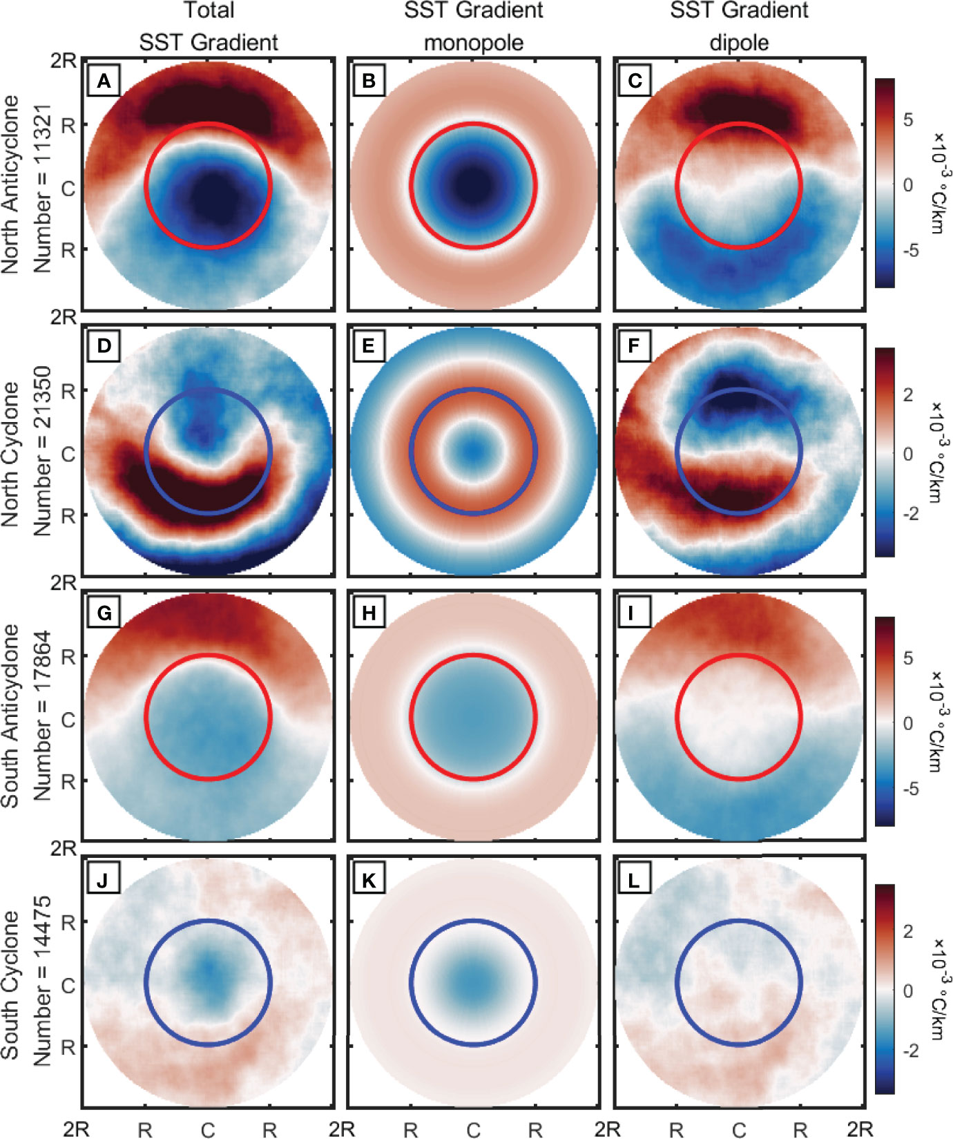
Figure 5 Composite of the SST gradient (×10-3°C/km) for (A–C and G–I) an anticyclone and (D–F and J–L) a cyclone in the (A–F) north and (G–L) south of the KE main path. The value within twice the radius is used for the composite, and the background field is removed in advance. The second (B, E, H, and K) and third (C, F, I, and L) columns correspond to the monopole and dipole features, respectively. The red (blue) circles represent the peripheries of anticyclonic (cyclonic) eddies. The total number of eddies used for the composite is shown for each row.
The total SST gradient anomaly is further separated into monopole (Figures 5B, E, H, K) and dipole (Figures 5C, F, I, L) features. For all eddies in the KE region, the dipole features show a negative SST gradient anomaly in the eddy center, and the SST gradient anomaly changes to positive outside the eddies. The zone with an SST gradient anomaly close to zero is located near the radius, although it is slightly inside (outside) the periphery of the eddy for a cyclone (anticyclone). The only exception is the cyclonic eddies in the north, where a positive circle is identified around the periphery of the eddy, while the remaining regions have negative values. The structure of the monopole is intuitively shown by calculating the averaged SST gradient anomaly over different distances from the center (Figure 6).
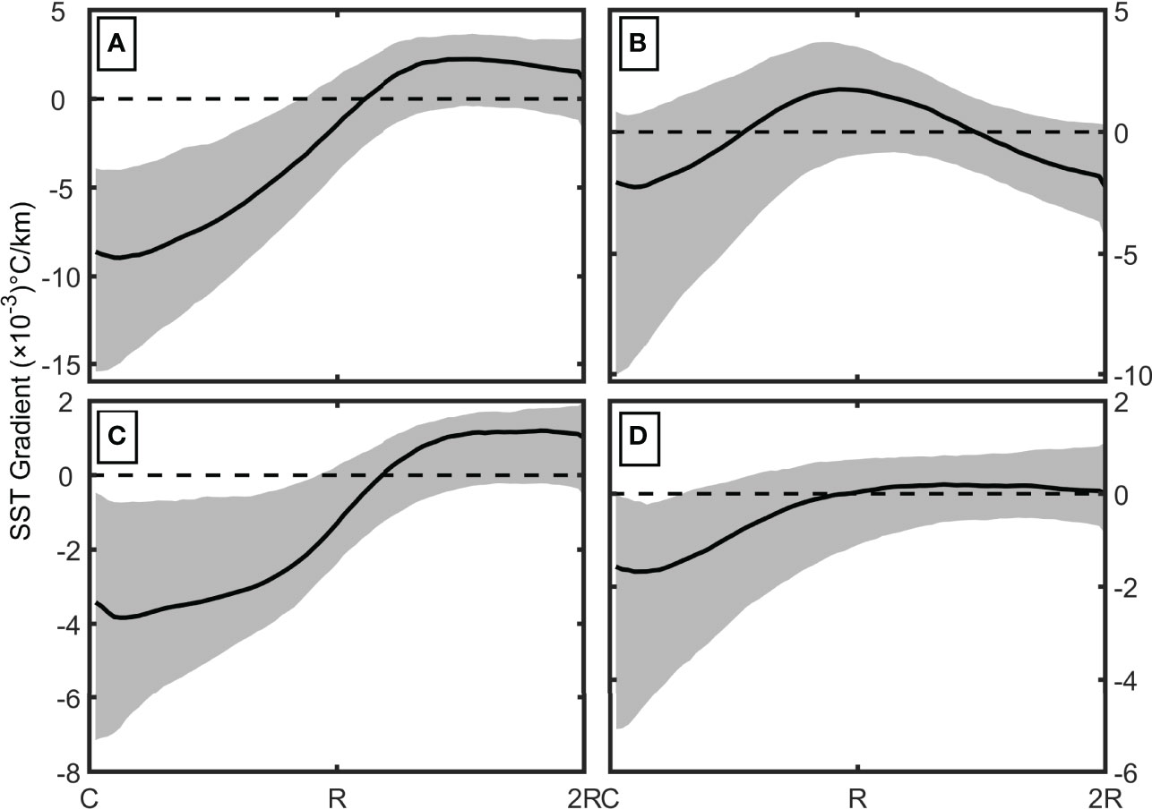
Figure 6 Averaged monopole of the SST gradient (×10-3°C/km) over different distances from the eddy center for (A) an anticyclone and (B) a cyclone in the north and for (C) an anticyclone and (D) a cyclone in the south. The horizontal dotted line represents the value of zero. The distance labeled on the x-axis shows the center C, radius (R) and twice the radii (2R) of the composited eddies. The gray shading represents the range between 30% and 70% of the total distribution.
The monopole feature in the eddies delineates the spatial variation in the SST gradient over different distances from the eddy centers (Figure 6). Consistent with the spatial pattern (Figure 5), the SST gradient anomaly for all eddies is that the KE region shows negative values near the center of the eddy. The SST gradient anomaly is larger in the anticyclonic eddies than in the cyclonic eddies; this pattern is particularly true for eddies in the north (Figure 6A). Outside the radius of the eddy, the SST gradient anomaly mostly becomes positive. The only exception is the cyclonic eddies in the north, where the SST gradient is positive around one radius of the eddy and negative near the eddy center and twice the radius (Figure 6B). Thus, these eddies are characterized by a unique distribution of three bands from the center to the surroundings. Based on this pattern, the cyclonic eddies in the north are divided into three bands for the following analysis.
Dipole features present very different patterns in anticyclonic (Figures 5C, I) and cyclonic (Figures 5F, L) eddies. For anticyclonic eddies, the SST gradient anomaly is positive and negative in the north and south, respectively, and their areas are approximately equal to each other. The cyclonic eddies in the north have prominent dipole features, where the positive (negative) gradient is advected anticlockwise toward the south (north) (Figure 5F). A similar but scattered pattern is identified for the cyclonic eddies in the south (Figure 5L).
In addition to the temporal evolution of the overall averaged SST gradient (Figure 4), the averaged SST gradient over different areas of eddies also varies over time (Figure 7). In particular, the averaged SST gradient is obtained for the area with a negative (positive) anomaly, which is mostly inside (outside) the radii of eddies (Figure 6). An exception is the cyclonic eddies in the north, where the SST gradient is positive for the area near the radius and negative for the remaining area (Figure 6B); thus, the group is divided into three areas, e.g., inside, middle and outside. The anticyclonic eddies in the north have a negative SST gradient inside eddies with a value of approximately -5.7×10⁻³°C/km and a positive SST gradient outside, e.g., 2.7×10⁻³°C/km, where both values are highly stable (Figure 7A). The feature is similar for the anticyclonic eddies in the south, although the values are smaller than those in the north (Figure 7C). The cyclonic eddies in the north are the most unique group, and the positive SST gradient in the middle is strengthened after generation and weakened before vanishing, which is associated with the large variation in the SST gradient inside and outside the eddies (Figure 7B). The cyclonic eddies in the south have a negative SST gradient of approximately -0.8×10⁻³°C/km, and the SST gradient outside is only approximately 0.2×10⁻³°C/km (Figure 7D). The difference in the SST gradient inside and outside anticyclonic eddies is more prominent than that in cyclonic eddies. For example, the mean SST gradient inside the anticyclone in the north (south) is greater than 4 ×10⁻³°C/km (3 ×10⁻³°C/km) but is less than 1 ×10⁻³°C/km for cyclones. However, the fluctuation in the SST gradient is more prominent for cyclones than anticyclones.
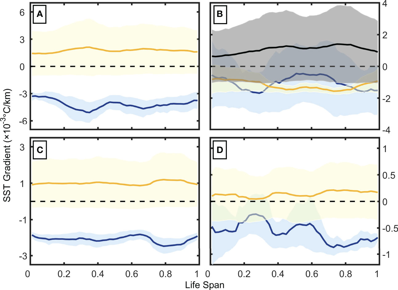
Figure 7 Temporal evolutions of the averaged SST gradient (×10-3°C/km) inside (blue) and outside (yellow) (A) anticyclonic and (B) cyclonic eddies in the north (the black line is the averaged SST gradient over the middle area of cyclonic eddies in the north) and (C) anticyclonic and (D) cyclonic eddies in the south. The gray, blue and yellow shading represents the standard error.
Discussion
The KE region is characterized by abundant mesoscale dynamics, such as eddies and fronts, which are common characteristics of boundary current systems (Yuan and Castelao, 2017). A front is generated when different water masses converge and can be identified via the SST gradient (Castelao and Wang, 2014). The spatial distribution of the SST gradient and eddies was investigated in this study, and the strong SST gradient region is mainly to the north of the KE and nearshore, especially near currents (Figure 1A). Due to the large stratification in the northern region, the corresponding SST and SST gradients are more sensitive to local upwelling, which introduces largely different features than those of surrounding water masses (Sato et al., 2016). Similarly, ocean currents, e.g., the Kuroshio and Oyashio Currents, can transport water with largely different features to their surroundings (Chelton et al., 2011a), leading to enhanced frontogenesis. Indeed, the frontal region with a strong SST gradient (Figure 1A) coincides well with the boundary of major currents, e.g., the Subarctic Front and the Kuroshio Bifurcation Front (Itoh and Yasuda, 2010). Mesoscale eddies are mainly distributed along the main path of the KE; in particular, the region with high eddy occurrence matches the large meanders of the KE main path (Ji et al., 2018). The meridional swing of the KE mainly occurs downstream of the KE, e.g., east of 155°E (Figure 3). As the meander of KE forces negative SSH anomalies southward, the KE rides over the ridges and introduces instability downstream of the KE (Qiu and Chen, 2005). The spatial variation in the SST gradient induced by eddies is fully investigated for the underlying dynamics.
The frontal variability induced by mesoscale eddies is quantitatively assessed in the KE region. Both anticyclonic and cyclonic eddies weakened (strengthened) the SST gradient inside (outside) the eddies (Figure 2), although their areas with elevated SST gradients were different. This result is at least related to the propagation of eddies and the associated dynamic processes. In particular, eddies have a westward propagation in the KE region (Itoh and Yasuda, 2010) such that their velocity on the east side is intensified by the steep SSH gradient, but the gentle SST gradient on the west side induces reduced velocity (Early et al., 2011). Hence, in anticyclonic (cyclonic) eddies, the increased equatorward (poleward) flow in the east transports more water southward (northward), while reduced poleward (equatorward) flow in the west transports less water northward (southward). As a result, the water masses diverge and induce upwelling in the north (south) of anticyclonic (cyclonic) eddies, converge in the south (north) and induce downwelling. As the local upwelling outcrops subsurface water to the surface, the upwelled water further expands and converges with surrounding surface water (Wang et al., 2021a). The resulting horizonal deformation between upwelled cold water and surrounding warm water at the surface subsequently elevates the SST gradient (Hoskins and Bretherton, 1972). Thus, the SST gradient north of anticyclonic (cyclonic) eddies is larger (smaller) than that south. Furthermore, eddy-related dynamic processes can introduce variations in the SST gradient. Because the largest contrast in SST takes place across the main path of the KE (Jing et al., 2019), the eddies in the main path induce prominent changes in SST. For example, the advection of anticyclonic eddies drives warm (cold) SST intrusion northward (southward) on their west side (east side) and elevates the corresponding SST gradient. This feature can be widely identified from the daily satellite observations of SST and location of eddies (not shown). Additionally, anticyclonic (cyclonic) eddies are mainly generated around the KE (Figure 1B) via instability in the meanders, which are mostly distributed to the north side (south side) of the main path (Ji et al., 2018). As the SST gradient generally increases toward the north (Figure 1A), the anticyclonic (cyclonic) eddies preferably maintain a large (small) SST gradient during its generation due to eddy trapping. Thus, the overall SST gradient is slightly larger in anticyclonic eddies than in cyclonic eddies. Additionally, because of the small equatorward propagation tendency of the anticyclonic eddies (Early et al., 2011), the large background SST gradient in the north shifts toward the north during meridional migration, leading to a further intensified SST gradient in the north of anticyclonic eddies (Figure 2A). In comparison, cyclonic eddies are moving northward (Early et al., 2011), and the larger background SST gradient will be gradually included in the northern eddies (Figure 2B). These dynamics introduce the complex spatial distribution of the SST gradient for each polarity of the eddies.
By further delineating eddies with different polarities to the north and south of the KE main path, eddies with different SST gradient backgrounds are individually investigated (Wang et al., 2021b). The temporal evolution of the SST gradient shows that they vary by more than 1×10⁻³°C/km over their lifetimes (Figure 4), and the variation is different for each group (Figure 5) due to the eddy-induced variability in the SST gradient (Yuan and Castelao, 2017). In particular, eddy trapping can separate the water mass from its origins and carry the water over a substantial time (Chelton et al., 2007). The SST gradient around the eddy periphery is becoming largely elevated due to the prominent difference in the SST trapped inside eddies during their generation and the SST outside eddies during their propagation (Figures 5A, D, G, I). In this case, monopole features are important, and the SST gradient gradually weakens due to eddy pumping and interior mixing (Figures 5B, E, H, K). Eddy strings can change the horizontal distribution of the background SST gradient (Chelton et al., 2011a), leading to a crescent shape with an enhanced SST gradient along the periphery (Figures 5C, F, I, L). The eddy-induced SST gradient is related to the background SST gradient, as many processes introduce the redistribution of the background field; thus, the SST gradient to the north of eddies is usually associated with a strengthened SST gradient.
The complex spatial distribution in the eddy-induced SST gradient (Figure 5) is revealed by calculating the monopole average of the eddy center, and the dipole feature induced by eddy advection is cancelled out. Except for northern cyclonic eddies, the eddies have a reduced SST gradient region inside their peripheries and a strengthened SST gradient outside, with the transitional zone mostly occurring near their radius (Figure 6). Thus, eddies mostly reduce the interior SST gradient, which contrasts with former studies where eddy-induced vertical transport results in anomalous changes in the SST and Chl-a within eddies (Gaube et al., 2014). The reduced SST gradient within eddies can also rely on eddy pumping, which introduces mixing and downwelling that result in relatively similar SST values (Siegel et al., 2011). The northern cyclonic eddies intensely strengthen the SST gradient along the southern periphery of eddies and overcome the reduction in the northern section (Figure 5D). Corresponding eddies are mostly generated by horizontal shear instability with a smaller scale and shorter lifetime (Ji et al., 2018). Considering the large background field in the SST (Wang et al., 2021b), these eddies originating from the KE converge with the surrounding water, leading to large differences along the eddy edge (Figure 5).
The averaged SST gradients outside of eddies are relatively stable because the background field is persistent (Figure 7). The values vary more prominently inside the eddy’s lifespan and are associated with several weak strengthening and weakening periods. This result is due in part to eddy-induced dynamics, such as upwelling, which transports subsurface water to the surface and results in a large contrast between internal cold water and warm water in the surroundings (Sun et al., 2020). Note that there is large variance during the lifespans of eddies, indicating that the feature is largely different in each case. The middle area in the northern cyclonic eddies shows a clear trend: increasing during the first half of their lifetime and decreasing afterward (Figure 7B). This trend might be related to the intensities of eddies, which also peak in the middle of the lifetime and can introduce upwelling to elevate the SST gradient between the interior and outside of eddies (Gaube et al., 2014). Thus, the change in the spatial pattern of eddies indicates the intensity of underlying dynamics, although multiple processes may simultaneously generate the same feature.
The KE has prominent interannual variability, classified as stable and unstable modes, and each mode can last for a few years (Qiu and Chen, 2011). The dynamic energy is different for the KE region, which is characterized by more (less) mesoscale dynamics during unstable (stable) modes (Qiu et al., 2014). However, the corresponding information is not included in this study. The investigated relationship between eddies and SST gradients focuses only on the ocean surface due to the limitation of remotely sensed data (Ritchie et al., 2003). The vertical structure of eddies can reach a depth of 160 meters (Sun et al., 2019), and the depth of the front can reach more than 300 m (Wang et al., 2020). Thus, the entire structure of eddies and fronts is not fully incorporated in the current study. With the development of autonomous underwater vehicles, e.g., glider and Argo floats, and high-resolution numerical models, the relationship between the mesoscale dynamics is expected to be resolved in a more comprehensive manner (Chai et al., 2020). The dependence between mesoscale dynamics can provide a complete picture for understanding the ocean.
Conclusion
In this study, the spatial distribution of the SST gradient and mesoscale eddies and their dependence are fully investigated. As the SST gradient is widely applied for gauging frontal activities, the information is new for understanding the relationship between major mesoscale dynamics, e.g., fronts and eddies. Furthermore, the northern regions have much larger SST gradients, and the eddies located to the north and south of the KE are separated to investigate their respective features without interference by the background field (Wang et al., 2021b). The spatial pattern and associated temporal variation are fully presented to assess the eddy-induced dynamics for modulating frontal activities. In comparison, former studies have mostly focused on investigating the impact of eddies on oceanic features, e.g., SST or Chl-a, but the influence on SST gradients or fronts is not yet available (Liu et al., 2020). Thus, the current study offers some new insight into the impact of eddies on modulating the distribution of frontal activities.
Data Availability Statement
The sea surface temperature dataset is obtained from National Aeronautics and Space Administration (NASA) via the Earth Science Data Systems (oceandata.sci.gsfc.nasa.gov/directaccess/MODIS-Aqua/Mapped/Daily/4km/sst4/). The global eddies dataset can be found via the Archiving, Validation and Interpretation of Satellite Oceanographic (AVISO) data (www.aviso.altimetry.fr/en/data/products/value-added-products/global-mesoscale-eddy-trajectory-product/meta2-0-dt.html); The sea surface height dataset is obtained from the Copernicus-Marine Environment Monitoring Service (resources.marine.copernicus.eu/product-detail/SEALEVEL_GLO_PHY_L4_MY_008_047/DATA-ACCESS).
Author Contributions
Data curation, RT and JX; writing, RT and YW; review of the manuscript, YY, JX, and WM; visualization, RT; funding, YW. All authors have read and agreed to the published version of the manuscript.
Funding
The study is funded by the National Natural Science Foundation of China (41730536 and 42176013) and the Scientific Research Fund of the Second Institute of Oceanography, MNR (No. QNYC2202).
Acknowledgments
We are very thankful to the National Aeronautics and Space Administration (NASA) for producing and distributing the sea surface temperature dataset and the Copernicus Marine Environment Monitoring Service (CMEMS) for producing the global eddy dataset and sea surface height dataset.
Conflict of Interest
The authors declare that the research was conducted in the absence of any commercial or financial relationships that could be construed as a potential conflict of interest.
Publisher’s Note
All claims expressed in this article are solely those of the authors and do not necessarily represent those of their affiliated organizations, or those of the publisher, the editors and the reviewers. Any product that may be evaluated in this article, or claim that may be made by its manufacturer, is not guaranteed or endorsed by the publisher.
References
Benitez-Nelson C. R., Bidigare R. R., Dickey T. D., Landry M. R., Leonard C. L., Brown S. L., et al. (2007). Mesoscale eddies drive increased silica export in the subtropical pacific ocean. Science 316, 1017–1021. doi: 10.1126/science.1136221
Castelao R., Wang Y. (2014). Wind-driven variability in sea surface temperature front distribution in the California Current System. Geophys. Res. Oceans 119 (3), 1861–1875. doi: 10.1002/2013JC009531
Chai F., Johnson K. S., Claustre H., Xing X., Wang Y., Boss E., et al. (2020). Monitoring ocean biogeochemistry with autonomous platforms. Nat. Rev. Earth Environ. 1, 315–326. doi: 10.1038/s43017-020-0053-y
Chelton D. B., Gaube P., Schlax M. G., Early J. J., Samelson R. M. (2011a). The influence of nonlinear mesoscale eddies on near-surface oceanic chlorophyll. Science 334, 328–332. doi: 10.1126/science.1208897
Chelton D. B., Schlax M. G., Samelson R. M., de Szoeke R. A. (2007). Global observations of large oceanic eddies. Geophys. Res. Lett. 34, L15606. doi: 10.1029/2007GL030812
Chelton D. B., Schlax M. G., Samelson R. M., de Szoeke R. A. (2011b). Global observations of nonlinear mesoscale eddies. Prog. Oceanogr. 91, 167–216. doi: 10.1016/j.pocean.2011.01.002
Early J. J., Samelson R. M., Chelton D. B. (2011). The evolution and propagation of quasigeostrophic ocean eddies. J. Phys. Oceanogr. 41, 1535–1555. doi: 10.1175/2011JPO4601.1
Frenger I., Münnich M., Gruber N., Knutti R. (2015). Southern ocean eddy phenomenology. J. Geophys. Res. Oceans 120, 7413–7449. doi: 10.1002/2015JC011047
Gaube P., Chelton D. B., Samelson R. M., Schlax M. G., O’Neill L. W. (2015). Satellite observations of mesoscale eddy-induced ekman pumping. J. Phys. Oceanogr. 45, 104–132. doi: 10.1175/JPO-D-14-0032.1
Gaube P., McGillicuddy D. J. Jr., Chelton D. B., Behrenfeld M. J., Strutton P. G. (2014). Regional variations in the influence of mesoscale eddies on near-surface chlorophyll. J. Geophys. Res. Oceans 119, 8195–8220. doi: 10.1002/2014JC010111
Hausmann U., Czaja A. (2012). The observed signature of mesoscale eddies in sea surface temperature and the associated heat transport. Deep Sea Res. Part I Oceanogr. Res. Pap. 70, 60–72. doi: 10.1016/j.dsr.2012.08.005
He Q., Zhan H., Xu J., Cai S., Zhan W., Zhou L., et al. (2019). Eddy-induced chlorophyll anomalies in the western south China Sea. J. Geophys. Res. Oceans 124, 9487–9506. doi: 10.1029/2019JC015371
Hoskins B., Bretherton F. (1972). Atmospheric frontogenesis models: Mathematical formulation and solution. J. Atmos. Sci. 29, 11–37. doi: 10.1175/1520-0469(1972)029<0011:AFMMFA>2.0.CO;2
Itoh S., Yasuda I. (2010). Characteristics of mesoscale eddies in the kuroshio–oyashio extension region detected from the distribution of the Sea surface height anomaly. J. Phys. Oceanogr. 40, 1018–1034. doi: 10.1175/2009JPO4265.1
Ji J., Dong C., Zhang B., Liu Y., Zou B., King G. P., et al. (2018). Oceanic eddy characteristics and generation mechanisms in the kuroshio extension region. J. Geophys. Res. Oceans 123, 8548–8567. doi: 10.1029/2018JC014196
Jing Z., Chang P., Shan X., Wang S.-P., Wu L.-X., Kurian J. (2019). Mesoscale SST dynamics in the Kuroshio-Oyashio extension region. J. Phys. Oceanogr. 49, 1339–1352. doi: 10.1175/JPO-D-18-0159.1
Kida S., Mitsudera H., Aoki S., Guo X., Ito S. I., Kobashi F., et al. (2015). Oceanic fronts and jets around Japan: A review. J. Oceanogr. 71, 469–497. doi: 10.1007/s10872-015-0283-7
Kostianoy A. G., Lutjeharms J. R. E. (1999). Atmospheric effects in the Angola-benguela frontal zone. J. Geophys. Res. 104 (C9), 20963–20970. doi: 10.1029/1999JC900017
Liu J., Wang Y., Yuan Y., Xu D. (2020). The response of surface chlorophyll to mesoscale eddies generated in the eastern south China Sea. J. Oceanogr. 76, 211–226. doi: 10.1007/s10872-020-00540-y
Ma J., Xu H., Dong C., Lin P., Liu Y. (2015). Atmospheric responses to oceanic eddies in the kuroshio extension region. J. Geophys. Res. Atmos. 120, 6313–6330. doi: 10.1002/2014JD022930
McWilliams J. C., Flierl G. R. (1979). On the evolution of isolated, nonlinear vortices. J. Phys. Oceanogr. 9, 1155–1182. doi: 10.1175/1520-0485(1979)009<1155:OTEOIN>2.0.CO;2>
Meng Y., Liu H., Lin P., Ding M., Dong C. (2021). Oceanic mesoscale eddy in the kuroshio extension: Comparison of four datasets. Atmos. Sci. Lett. 14, 100011. doi: 10.1016/j.aosl.2020.100011
Mizobata K., Saitoh S. I., Shiomoto A., Miyamura T., Shiga N., Lmai K., et al. (2002). Bering Sea Cyclonic and anticyclonic eddies observed during summer 2000 and 2001. Prog. Oceanogr. 55, 65–75. doi: 10.1016/S0079-6611(02)00070-8
Mizuno K., White W. B. (1983). Annual and interannual variability in the kuroshio current system. J. Phys. Oceanogr. 13, 1847–1867. doi: 10.1175/1520-0485(1983)013<1847:AAIVIT>2.0.CO;2
Nurser A. J. G., Zhang J. W. (2000). Eddy-induced mixed layer shallowing and mixed layer/thermocline exchange. J. Geophys. Res. 105 (C9), 21851–21868. doi: 10.1029/2000JC900018
Qiu B. (2002). The kuroshio extension system: Its large-scale variability and role in the midlatitude ocean-atmosphere interaction. J. Oceanogr. 58, 57–75. doi: 10.1023/A:1015824717293
Qiu B., Chen S. (2005). Variability of the kuroshio extension jet, recirculation gyre, and mesoscale eddies on decadal time scales. J. Phys. Oceanogr. 35, 2090–2103. doi: 10.1175/JPO2807.1
Qiu B., Chen S. (2011). Effect of decadal kuroshio extension jet and eddy variability on the modification of north pacific intermediate water. J. Phys. Oceanogr. 41, 503–515. doi: 10.1175/2010JPO4575.1
Qiu B., Chen S., Schneider N., Taguchi B. (2014). A coupled decadal prediction of the dynamic state of the kuroshio extension system. J. Clim. 27, 1751–1764. doi: 10.1175/JCLI-D-13-00318.1
Ritchie J., Zimba P., Everitt J. H. (2003). Remote sensing techniques to assess water quality. Photogramm Eng. Remote Sens. 69, 695–704. doi: 10.14358/PERS.69.6.695
Rykaczewski R. R., Dunne J. P., Sydeman W. J., García-Reyes M., Black B. A., Bograd S. J. (2015). Poleward displacement of coastal upwelling-favorable winds in the ocean's eastern boundary currents through the 21st century. Geophys. Res. Lett. 42, 6424–6431. doi: 10.1002/2015GL064694
Sato N., Nonaka M., Sasai Y., Sasaki H., Tanimoto Y., Shirooka R. (2016). Contribution of sea-surface wind curl to the maintenance of the SST gradient along the upstream kuroshio extension in early summer. J. Oceanogr. 72, 697–705. doi: 10.1007/s10872-016-0363-3
Shan X., Jing Z., Gan B., Wu L., Chang P., Ma X., et al. (2020). Surface heat flux induced by mesoscale eddies cools the kuroshio-oyashio extension region. Geophys. Res. Lett. 47, e2019GL086050. doi: 10.1029/2019GL086050
Siegel D. A., Peterson P., McGillicuddy D. J., Maritorena S., Nelson N. B. (2011). Bio-optical footprints created by mesoscale eddies in the Sargasso Sea. Geophys. Res. Lett. 38, L13608. doi: 10.1029/2011GL047660
Sugimoto T., Tameishi H. (1992). Warm-core rings, streamers and their role on the fishing ground formation around Japan. Deep Sea Res. Part A. Oceanographic Res. Papers 39, S183–S201. doi: 10.1016/S0198-0149(11)80011-7
Sun B., Liu C., Wang F. (2020). Eddy induced SST variation and heat transport in the western north pacific ocean. J. Ocean. Limnol. 38, 1–15. doi: 10.1007/s00343-019-8255-1
Sun W., Dong C., Tan W., He Y. (2019). Statistical characteristics of cyclonic warm-core eddies and anticyclonic cold-core eddies in the north pacific based on remote sensing data. Remote Sens. 11, 208. doi: 10.3390/rs11020208
Tatebe H., Yasuda I. (2004). Oyashio southward intrusion and cross-gyre transport related to diapycnal upwelling in the Okhotsk Sea. J. Phys. Oceanogr. 34, 2327–2341. doi: 10.1175/1520-0485(2004)034<2327:OSIACT>2.0.CO;2
Wang J., Mao K., Chen X., Zhu K. (2020). Evolution and structure of thekuroshio extension front in spring 2019. J. Mar. Sci. Eng. 8, 502. doi: 10.3390/jmse8070502
Wang Y., Castelao R. M., Yuan Y. (2015). Seasonal variability of alongshore winds and sea surface temperature fronts in Eastern boundary current systems. J. Geophys. Res. Oceans 120, 2385–2400. doi: 10.1002/2014JC010379
Wang Y., Liu J., Liu H., Lin P., Yuan Y., Chai F. (2021a). Seasonal and interannual variability in the sea surface temperature front in the eastern pacific ocean. J. Geophys. Res. Oceans 126, e2020JC016356. doi: 10.1029/2020JC016356
Wang Y., Tang R., Yu Y., Ji F. (2021b). Variability in the Sea surface temperature gradient and its impacts on chlorophyll-a concentration in the kuroshio extension. Remote Sens. 13, 888. doi: 10.3390/rs13050888
Wang Y., Zhang H. R., Chai F., Yuan Y. (2018). Impact of mesoscale eddies on chlorophyll variability off the coast of Chile. PLoS One 13, e0203598. doi: 10.1371/journal.pone.0203598
Xi J., Wang Y., Feng Z., Liu Y., Guo X. (2022). Variability and intensity of the sea surface temperature front associated with the kuroshio extension. Front. Mar. Sci. 9. doi: 10.3389/fmars.2022.836469
Yang P., Jing Z., Sun B., Wu L., Qiu B., Chang P., et al. (2021). On the upper-ocean vertical eddy heat transport in the kuroshio extension. part II: Effects of air-Sea interactions. J. Phys. Oceanogr. 51, 3297–3312. doi: 10.1175/JPO-D-20-0068.s1
Yasuda I. (2003). Hydrographic structure and variability in the kuroshio-oyashio transition area. J. Oceanogr. 59 (4), 389–402. doi: 10.1023/A:1025580313836
Keywords: mesoscale eddies, sea surface temperature gradient, Kuroshio Extension, monopole and dipole features, main path of Kuroshio Extension
Citation: Tang R, Yu Y, Xi J, Ma W and Wang Y (2022) Mesoscale eddies induce variability in the sea surface temperature gradient in the Kuroshio Extension. Front. Mar. Sci. 9:926954. doi: 10.3389/fmars.2022.926954
Received: 23 April 2022; Accepted: 30 June 2022;
Published: 27 July 2022.
Edited by:
Guangchao Zhuang, Ocean University of China, ChinaReviewed by:
Zhao Jing, Ocean University of China, ChinaHatsumi Nishikawa, The University of Tokyo, Japan
Copyright © 2022 Tang, Yu, Xi, Ma and Wang. This is an open-access article distributed under the terms of the Creative Commons Attribution License (CC BY). The use, distribution or reproduction in other forums is permitted, provided the original author(s) and the copyright owner(s) are credited and that the original publication in this journal is cited, in accordance with accepted academic practice. No use, distribution or reproduction is permitted which does not comply with these terms.
*Correspondence: Yuntao Wang, eXVudGFvLndhbmdAc2lvLm9yZy5jbg==