 Weiqi Li
 Xiangqian Zhou
 Jianzhong Ge
 Pingxing Ding1
94% of researchers rate our articles as excellent or good
Learn more about the work of our research integrity team to safeguard the quality of each article we publish.
Find out more
ORIGINAL RESEARCH article
Front. Mar. Sci. , 20 July 2022
Sec. Coastal Ocean Processes
Volume 9 - 2022 | https://doi.org/10.3389/fmars.2022.926738
Estuarine plume frontal zones typically form a vertical two-layer structure with low-salinity and a high-temperature plume during the summertime. However, two field surveys in the Changjiang River Estuary and its adjacent shelf waters identified a significant surface cold-water zone (CWZ) formation in the summers of 2014 and 2015. The sea surface temperature of the CWZ was 4°C lower than the multi-year summer average. Satellite images showed that the CWZ mainly appeared in the Yangtze Shoal during the periods of July 1–17, 2014, and July 3–19, 2015. A three-dimensional physical-biogeochemical coupled model was used to explore the formation mechanism of the CWZ. Our investigation revealed that an uncharacteristic northerly wind during the southerly monsoon resulted in a significant onshore retreat of the plume front. Vertical tidal mixing is stronger than the decreased stratification in the former plume-covered region, which resulted in the formation of the CWZ. This process was accompanied by relatively lower net heat flux, which also promoted CWZ formation. The formation of CWZ had a strong ecological impact; enhanced vertical mixing transported nutrients from the lower layer to the surface column, relaxing the CWZ’s phosphate limitation. CWZ formation also increased the depth of the mixed layer and turbidity level in the water column, forming a temporary light limitation in the center. At the margin of the CWZ, it formed a patch with a high concentration of chlorophyll a. The underwater light was sufficient once the plume was restored and the CWZ was stratified again, and the phytoplankton grew rapidly in the center of the CWZ.
In the larger rivers of the world, such as the Changjiang, Mississippi, and Amazon Rivers, low-salinity water usually floats on the upper layer in the form of low-salinity plumes during the wet summer season, and their expansion ranges can reach tens or hundreds of kilometers (Smith and Demaster, 1996; Lohrenz et al., 1999; Ge et al., 2013). In addition, due to the surface warming effect caused by strong shortwave radiation during the summer, stratified water in the upper water layer usually has a high sea surface temperature (SST) relative to that in well-mixed regions (Simpson and Hunter, 1974). The higher SST also increases the intensity of stratification. Therefore, it is generally believed that, influenced by the freshwater discharge extension and solar radiation during the summer, estuarine offshore regions are usually stratified due to lower salinity and higher SST, particularly in estuaries with abundant runoff (Simpson et al., 1991; Zhu et al., 2016).
The stratification of water due to differences in vertical salinity and temperature has an important influence on the vertical exchange of matter and energy, as well as ecological and biogeochemical processes (Simpson et al., 1981; Chen et al., 1999; Wei et al., 2016; Zhabin et al., 2019). Stratification can inhibit the resuspension of sediment, thus reducing the attenuation of the underwater light penetration, and promoting the growth of phytoplankton (Geyer, 1993; Cloern et al., 2017; Ge et al., 2020a). Stratification also restricts the transport of the water with a high concentration of nutrients from the bottom to the surface (Prasanna Kumar et al., 2002; Zhu et al., 2016), usually resulting in a significant depletion of one or two nutrients in the upper column due to phytoplankton growth (Gao et al., 2015; Ge et al., 2020a). Consequently, the significant nutrient limitation can occur, which is an important factor in restraining phytoplankton bloom during the summer season in the shelf water zone (Tseng et al., 2014; Li et al., 2021).
Although the low-salinity plume is the dominant physical and ecological feature in estuaries, the occurrence of cold-water zones (CWZs) in coastal and inner shelf regions is possible (Simpson and Hunter, 1974; Lü et al., 2010; Guo et al., 2014; Ren et al., 2014). The tidal mixing front (TMF) and upwelling are the two most common mechanisms of the summer surface CWZ in estuaries and shelf water zones (Sousa et al., 2008; Lü et al., 2010; Sapozhnikov et al., 2011; Ren et al., 2014). The TMF separates shelf water into well-mixed and stratified water (Simpson and Hunter, 1974; Bowers and Lwiza, 1994). The different conditions of water on both sides of the TMF can produce spatial discontinuity of SST (Simpson and Hunter, 1974; Huang et al., 2018). Low SST generally occurs at the proper depth of the mixed region around the TMF (Lü et al., 2010). During summer, tidal mixing induced by the friction between the tidal current and seabed is the most important driving force to break or decrease stratification and enhance vertical mixing (Simpson et al., 1991; Scully and Geyer, 2012). In shelf regions, where the diluted water does not have a strong effect, the location of the thermal TMF is relatively stable (Simpson and Hunter, 1974; Simpson et al., 1978).
For estuaries and adjacent shelf waters affected by large rivers, the interaction between the plume-induced stratification and tidal mixing is more complicated (Simpson et al., 1991). The low-salinity plume has the lateral boundary as the plume front (Li et al., 2021). However, the thermal heat flux from solar radiation is relatively spatially uniform, even when clouds are present (Simpson et al., 1991). Additionally, the plumes have considerable spatial and temporal variations due to fluctuations in river discharge and atmospheric wind fields (Chang and Isobe, 2003; Liu and Feng, 2012). These spatio-temporal variations of plumes might lead to a rapid change from vertical mixing to stratification, subsequently impacting environmental factors, such as salinity, temperature, and nutrients.
During the flood seasons of large rivers, stratified plumes usually have great spatial coverage with relatively higher SST (de Boer et al., 2009; Zhang et al., 2020). With abundant freshwater discharge and strong surface warming effects, the occurrences of surface CWZs are quite low around the plume-covered regions during summertime as long as there is no strong upwelling system. In this study, we identified extraordinary surface CWZs from field survey data and examined the formations and breakdown processes of strong CWZs off the Changjiang Estuary under large runoff during the summertime. The effect of this type of CWZ on the phytoplankton was also investigated.
The study region included the Changjiang River Estuary (CRE) and its adjacent shelf waters (121°E–124.5°E, 28.5°N–33°N, shown as a red box in Figure 1A). The Changjiang River is Asia’s largest river, depositing ample nutrient-rich and turbid freshwater into the CRE and its adjacent shelf water during the summer (June–August), with an average runoff rate of approximately 45,000 m3·s−1 between 1951 and 2018 (river discharge was measured at Datong station: www.cjh.com.cn). Affected by the southerly summer monsoon, the Changjiang plume mainly extends northeastward (Beardsley et al., 1985) and covers the Yangtze Shoal (YS) (in Figure 1A, the isohaline is redrawn from the Marine Atlas of Bohai Sea, Yellow Sea, East China Sea). As the outer boundary of the plume, the plume front can describe the region that is most influenced by the low-salinity plume (Chen et al., 1999; Li et al., 2021). There are usually strong pycnoclines on the landside of the plume front, which are caused by the surface low-salinity plume and bottom saline water (Chen et al., 1999; Ge et al., 2020a). The plume front in the CRE and its adjacent waters is characterized by a relatively high salinity gradient (> 0.1 km−1) with a sea surface salinity (SSS) range from 25 to 31 (Hu et al., 1995; Chen et al., 1999; Li et al., 2021). The water depth of the CRE and its coastal area is shallow (<20 m) and increases dramatically to ~50 m at approximately 122°E–122.5°E (Figure 1B). The YS (122.5°E–124.5°E, 31.5°N–33°N) is located in the northeastern region off the CRE, which is relatively shallow, with a water depth of 30–50 m. The submerged river valley (SRV) and East China Sea Shelf are located in the southeastern area off the CRE, where the water depth is greater (50–80 m).
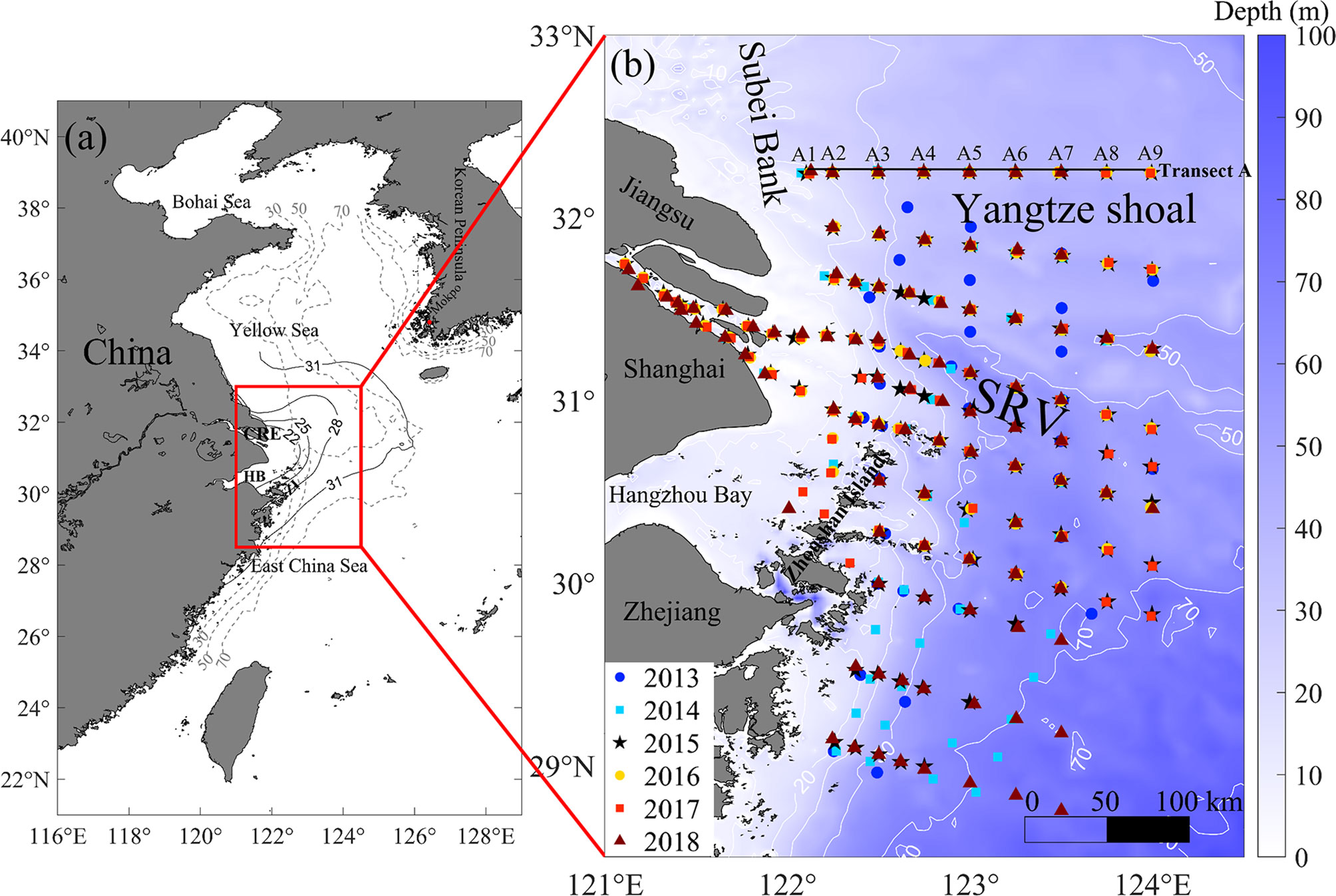
Figure 1 The location of the Changjiang River Estuary (CRE), East China Sea, and adjacent regions (A), and enlarged view of the CRE and adjacent shelf water zone including summer survey sites from 2013–2018 (B). The black solid isolines are climatological summer sea surface salinity digitalized from Marine Atlas of Bohai Sea, Yellow Sea East China Sea (1992). The grey dashed lines represent water depths of 30 m, 50 m, and 70 m, respectively. SRV, Submerged River Valley; HB, Hangzhou Bay. The transect A1 was investigated from Jiangsu coastal region (site A1) to Yangtze Shoal (site A9).
Previous studies have reported that summer surface CWZs or relatively lower SSTs mainly occur in coastal areas (Zhu, 2003; Lü et al., 2010; Ren et al., 2014). For example, the upwelling region around the Zhoushan Island (122.2°E-123°E, 29°N-31°N) could have an SST that is 3°C lower than the temperature of the surrounding water (Lü et al., 2006); in addition, a banded surface CWZ related to the TMF was found in the Jiangsu coastal region (121.5°E–122.5°E, 32°N–34°N) (Lü et al., 2006; Ren et al., 2014). The shelf water region between 123°E–124.5°E (including YS, SRV, and the East China Sea Shelf) usually has strong stratification due to low-salinity and high-SST coverage during the summer, and no CWZ was observed in previous studies (Lü et al., 2010; Guo et al., 2014; Ren et al., 2014). Thus, the CRE and its adjacent shelf water were suitable for studying the possible formation mechanism of summer surface CWZs in the shelf water zone.
Six survey cruises were conducted during summers (July) for the period 2013–2018 in the CRE and its adjacent shelf (Figure 1B). The surveys mostly followed the same 99 sites. These sites were distributed from the CRE to the inner shelf. Salinity, temperature, and density were measured using a CTD-SBE 25 profiler (Sea-Bird Scientific, Bellevue, WA, USA). Niskin bottles were used to collect the surface (0–2 m), middle (0.5 × water depth), and bottom (2 m above the seabed) seawater samples from each site. In order to obtain the concentration of total suspended matter (TSM), a Whatman filter (0.7 μm) was used to filter 1-L seawater samples. Then, the filter membrane was dried at 60°C for approximately 48 h and weighed using an electronic balance to calculate the TSM concentration. Whatman cellulose acetate membranes (0.45 μm) were used to filter 500 ml seawater samples; the filter membranes were then stored in a refrigerator at −20°C for the analysis of chlorophyll a (Chl-a) concentration. The Chl-a was extracted using 15 ml of 90% acetone in the dark at 4°C for approximately 24 h. Then, the Chl-a concentration was measured using a Trilogy Laboratory fluorometer (Turner Design, San Jose, CA, USA ). The concentrations of nutrients, including dissolved inorganic nitrogen (DIN), dissolved silicate (DSi), and dissolved inorganic phosphate (DIP), were measured using a San++ continuous flow analyzer (SKALAR, Netherlands).
The Group for High-Resolution SST (GHRSST) data with a spatial resolution of 0.011°, was used to analyze the spatial and temporal variation of the daily SST during summers for 2005–2018. Additionally, surface wind at 10 m above sea surface and net heat flux provided by the European Centre for Medium-Range Weather Forecasts (ECMWF) Reanalysis v5 (ERA5) were used to determine the atmospheric condition. These data had a spatial resolution of 0.125° and temporal intervals of 3 h. The daily average wind field and net heat flux were calculated based on the ECMWF data. The climatological daily average SST, wind, and net heat flux for June 15 to July 31 for the years 2005–2018 were calculated using ECMWF and GHRSST data. Furthermore, the summertime anomalies of these variables were also determined.
The three-dimensional physical-biogeochemical coupled model established by Ge et al. (2020a, 2020b) was used in this study to simulate the physical and ecological dynamic processes in the CRE and its adjacent shelf waters. The Finite Volume Community Ocean Model (FVCOM) provided the calculations for the hydrodynamics, while biogeochemical simulations were performed by the European Regional Seas Ecosystem Model (ERSEM; Butenschön et al., 2016). FVCOM and ERSEM were coupled through the Framework for Aquatic Biogeochemical Models (FABM; Bruggeman and Bolding, 2014). The triangular network of model systems covered the Changjiang Estuary and inner shelf of the East China Sea with a spatial resolution from ~10 km along the lateral boundary to 500–1000 m in the river mouth. The water column was discretized into 10 uniformly distributed terrain-following layers. This model was simulated from January 1, 1999, to December 31, 2018 (Ge et al., 2020b), and the model system was driven by ECMWF atmospheric forcing and assimilated with daily SST from GHRSST (Chen et al., 2003). Eight astronomical tide components (M2, S2, K2, N2, O1, K1, Q1, and P1) were specified by TPXO 7.2 Global Tidal Solution at the open boundary (Egbert and Erofeeva, 2002). Daily HYCOM/NCODA data with a spatial resolution of 1/12° were interpolated into the boundary grid. The daily Changjiang river discharge and sediment measured at Datong Hydrological Station were specified at the river boundary. The environmental factors (including salinity, temperature, TSM, and nutrient concentrations) and Chl-a concentration simulated by the FVCOM-ERSEM coupling model were verified by the observed data. For more details on this model, see Ge et al. (2020a); Ge et al. (2020b).
The vertical average irradiance in the mixing layer (Im) was used to quantify the threshold of light-limitation, which is calculated according to the following formula:
where I0 is the surface intensity of photosynthetically available radiation (PAR) obtained from the ECMWF; the mixed layer depth (MLD) was determined by the vertical density profile of CTD from the surveys of 2013–2018 according to Chu and Fan (2011); k denotes the attenuation coefficient of light underwater, which changed with the variation of TSM and Chl-a concentration, and is calculated as follows (Cloern, 1987):
The three terms on the right side represent the light attenuation by the water, phytoplankton, and TSM, respectively. Using Zhao and Guo’s study (2011) as a reference, the light attenuation coefficients of water (kw) and phytoplankton (kChl-a) were 0.04 m−1 and 0.0138 m2·mg−1 Chl-a, respectively. The light attenuation coefficient of TSM was calculated using the average value (0.0608 m2·g−1) in the CRE and the adjacent shelf (Zhang et al., 2003; Zhang et al., 2004; Zhu et al., 2010; He et al., 2011; Zhao and Guo, 2011). When Im<80 µmol photons m−2 s−1, the light limitation occurred (Riley, 1957; Hitchcock and Smayda, 1977; Thompson, 1999; Lin et al., 2019).
As the outer boundary of the Changjiang plume, the plume front is characterized by a relatively high SSS gradient and medium SSS. According to Li et al. (2021), the definition of plume front is the area with an SSS gradient of greater than0.1 km−1 and an SSS from 25 to 31. In order to determine the location of the plume front, the SSS was interpolated to a fixed regular grid with a resolution of 0.05°, and the spatial gradient of SSS was calculated as follows:
The buoyancy frequency () and potential energy anomaly (Ø) were used to estimate the stratification of the water body. The buoyancy frequency is calculated as follows:
where g represents the local gravitational acceleration, and ρ0 is the water density.
The potential energy anomaly Ø is calculated as follows:
where h is the total water depth, represents the vertical average density, z is the water depth, and ρ is the density value at different water depths. The smaller the value of Ø, the more fully the water is mixed. When Ø<10 J·m3, the water is considered to be fully mixed. The vertical average turbulent kinetic energy (VATKE) is calculated according to flowing equation:
where q2 is the turbulent kinetic energy. The q2was calculated using FVCOM and linearly interpolated to a water layer with a vertical interval of 1 m.
The environmental factors of SSS, SST, DIN, DSi, DIP, MLD, Im, as well as Chl-a concentrations for the summers of 2013–2018, were interpolated to a regular grid with a spatial resolution of 0.05°× 0.05°. The multi-year summer average spatial patterns of environmental factors and Chl-a concentrations were calculated at this regular grid. The multi-year average SSS showed that the Changjiang plume primarily extended northeast off the CRE, and only a small part of the plume flowed to the southeast, distributed along the coast (Figure 2A). The plume front in the northeast area (north of 31.5°N) off the CRE, located in the offshore region between 123.5°E–124°E and 31°N–32.5°N. However, in the summer of 2014, the Changjiang plume mainly flowed southeastward, and the plume front substantially receded towards the shore (Figure 2B). The plume front in 2015 was also much closer to the land and was located between 122.2°E and 123.3°E (Figure 2C).
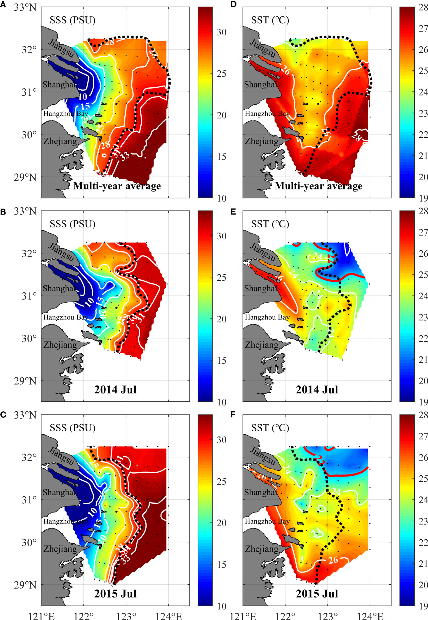
Figure 2 Spatial distributions of the summer sea surface salinity (SSS, A–C) and sea surface temperature (SST, D-F) around CRE and its adjacent waters of multi-year average (2013–2018, first row), 2014 (middle row), and 2015 (bottom row). Black dashed lines represent the boundaries of the plume front, and the red solid lines are the isothermal contour of 22°C which represents the boundary of the cold-water zone (CWZ).
The relatively lower SST (24°C–26°C) of the multi-year average appeared in the coastal area between 122°E–123°E and 29.5°N–32.5°N, and the SST was relatively higher (26°C–28°C) in the CRE and shelf water (Figure 2D). However, the spatial patterns of SST in the summer of 2014 were quite different from the multi-year average distribution (Figure 2E). The lowest SST level reached less than22°C, occurring in the region northeast off the CRE with a range of 122.5°E–124°E, 31.5°N–32.5°N. The spatial distribution of SST in 2015 was similar to that in 2014, with the lowest SST also occurring in the YS off the plume front (Figure 2F). Therefore, the CWZ was identified by the bounded area with an SST of<22°C. The western boundary of the CWZ (isothermal line of 22°C) was spatially matched with the summer plume fronts of 2014 and 2015 (Figures 2E, F).
Using the measured data at observation sites in the CWZ in 2014 and 2015, the mean surface and bottom salinity and temperature, and the surface and bottom difference were calculated (Table 1). The average SST of the CWZ was 20.2±0.3°C in 2014 and 21.4±0.9°C in 2015, which was ~4°C lower than multi-year average SST, and ~6°C lower than the average SST in 2013 and 2016–2018. The interannual variation of SST in other regions, such as the CRE and the shelf water southeast off the CRE, were relatively small (less than 1°C) (Figures 2D–F).
Transect A (black line as in (Figure 1B) was selected to explore the hydrodynamic characteristics of the CWZ, including the vertical distribution of salinity, temperature, and buoyancy frequency (N2) (Figure 3 and Figure S1 in Supplementary Material). In the CWZ (123.2°E–124°E, A6–A9), the vertical distributions of salinity and temperature were uniform in 2015 (Figures 3A, B). The maximum N2 in the CWZ was ~0.004 s−2 (Figure 3C). There was a similar vertical distribution of salinity, temperature, and buoyancy frequency in 2014 (Figures S1A–C) and 2015 (Figures 3A–C). These results indicated that the vertical mixing was dominant in whole water column and there was almost no stratification in the CWZ. However, in the summer of other years, such as 2016, stratification was evident, with strong halocline and thermocline near the depth of 5–10 m, with N2>0.015 s−2 ( Figures 3D–F). The stratification was also stronger in the summer of 2017 with maximum N2 of 0.03 s−2 (Figures S1D–F). In the summer of 2013 and 2016–2018, the average ΔS (5.9±2.9) and ΔT (6.6±1.5°C) were significantly higher than those in the summer of 2014 (ΔS=0±0; ΔT=0.2±0.1°C) and 2015 (ΔS=0.4±0.3; ΔT=0.9±0.7°C; Table 1). Furthermore, the relatively high ΔS and ΔT in the multi-year summer average indicate that strong stratification is a common feature in the YS.
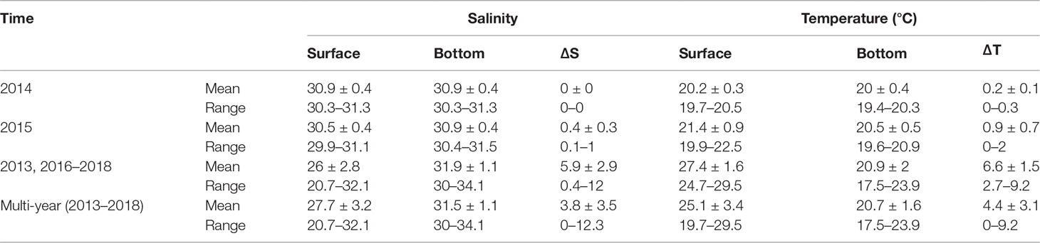
Table 1 Mean, standard deviations, and ranges of salinity and temperature at surface, bottom, and the absolute difference between surface and bottom measured at sites in the CWZ (122.5°E–124°E, 31.5°N–32.5°N).
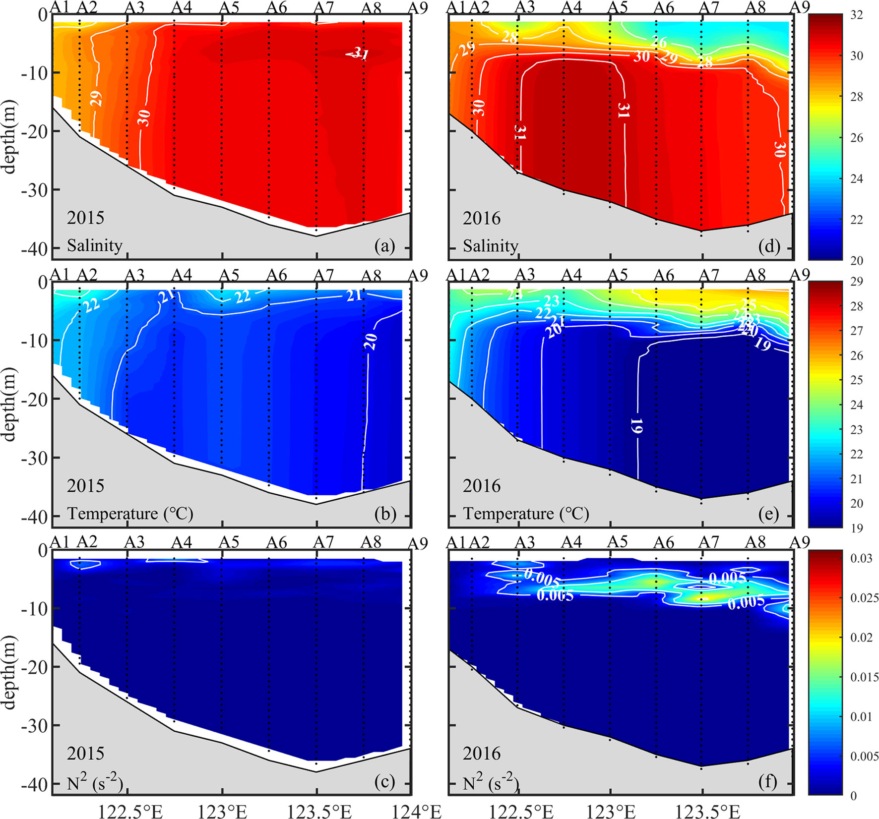
Figure 3 Vertical distributions of salinity (A, D), temperature (B, E), and squared buoyancy frequency (C, F) along Transect A (32.25°N) in summer of 2015 (A–C) and 2016 (D–F).
To reveal the full spatial extent of the CWZ in the YS, the SST distributions in the East China and Yellow Seas were presented using 10-day average satellite data. The satellite SST data showed that there was broad coverage of CWZ in the YS and adjacent regions from July 1–10, 2014 (Figure 4A). By the July 11-21, the CWZ only existed in the YS ( Figure 4B), and the CWZ area was significantly reduced after July 15 (Figure S2 in Supplementary Material). From July 21-31, 2014, the SST in the YS was much higher (>26°C) and the CWZ completely disappeared (Figure 4C)
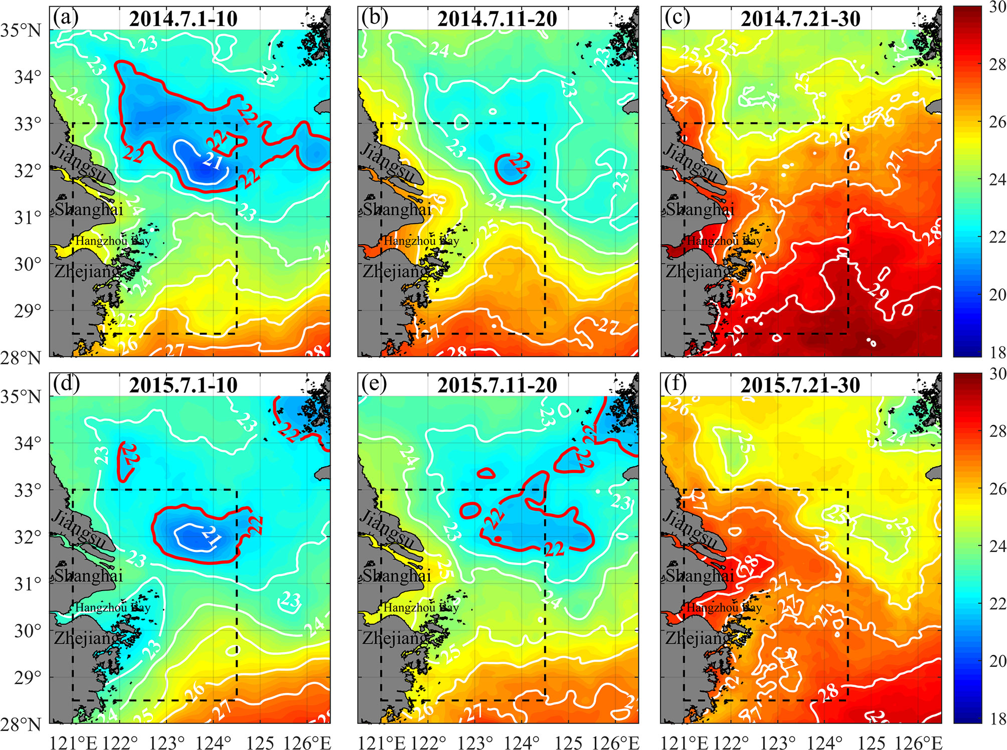
Figure 4 Spatial distributions of the 10-day averaged satellite SST from July 1-10, July 11-20, and July 21-30 of 2014 (A–C) and 2015 (D–F) (red line represents the boundary of CWZs, black dashed box indicates the survey area shown in Figure 1B).
From July 1-10, 2015, there were three CWZs in the YS (122.8°E–125°E, 31.5°N–32.8°N), Jiangsu coastal region (122°E–122.4°E, 33°N–34°N), and the southwest region of the Korean Peninsula (125.2°E–126.5°E, 34°N–35°N) ( Figure 4D). The CWZ still existed in the YS from July 11-20 ( Figure 4E), but completely disappeared in the following period (Figure 4F). The CWZs in the Jiangsu coastal region and southwest region of the Korean Peninsula have been examined in previous studies that were related to TMF and tide-induced upwelling (Lü et al., 2010; Ren et al., 2014; Wei et al., 2016). However, the CWZ in the YS during summer has not been documented and its mechanisms remain unknown.
Through limited observations, we identify two occurrences of CWZ from 2013 to 2018. To further reveal the occurrence frequency and duration of CWZs in the YS, the temporal variation of daily SST of June 15–July 31 from 2005 to 2018 at the center of CWZ (123.5°E, 32°N), as well as its anomalies, are shown in Figure 5A. The SST typically increased gradually from June 15 to July 31 in most years. However, for the duration of June 17 to July 17 in 2014 and June 16 to July 19 in 2015, SST maintained in a low level of 19°C–22.3°C without significant increase. The SST anomalies were between −2°C and −5°C between June 1–17 of 2014, and July 3–19, 2015, demonstrating that the SST during these periods was much lower than the multi-year average SST. Thus, the period with lower SST (<22°C) and SST anomalies (<−2°C) indicated the formation phase of CWZs (shaded regions). With these criteria, there were three major occurrences of CWZ in the YS in the summer from 2005 to 2018, including the longer presence (17 days) of CWZ only appeared in 2014 and 2015, meanwhile, there was also a shorter (8 days) formation of CWZ on June 15–22, 2011. During July 18–31 of 2014, and July 20–31 of 2015, the SST increased rapidly and the corresponding SST anomaly changed from negative to positive, demonstrating the breakdown phase of the CWZ.
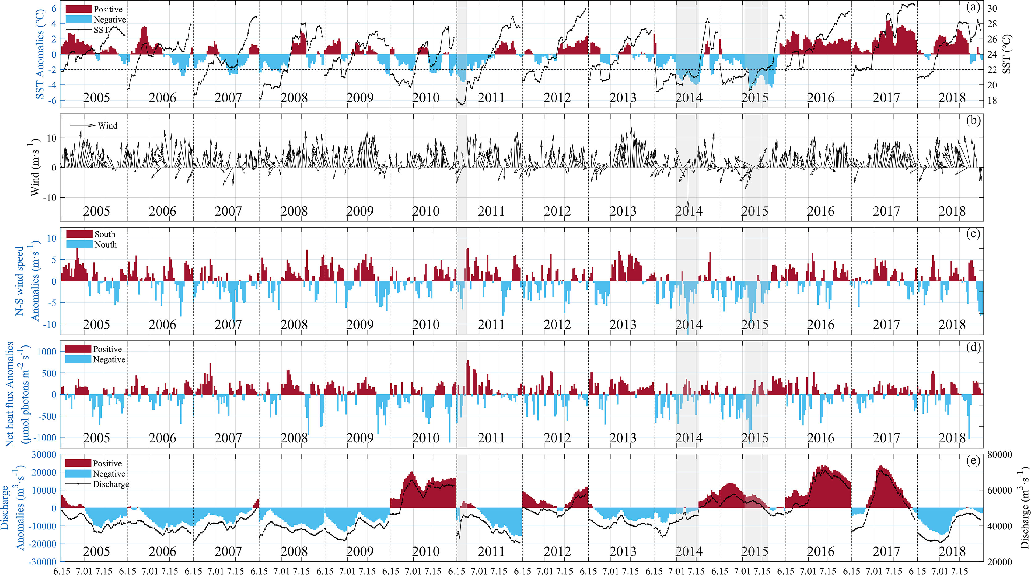
Figure 5 Temporal variations of daily SST and SST anomalies (A), wind (B), North-South (N-S) speed anomalies (C), and net heat flux anomalies (D) at central of the CWZ (123.5°E, 32°N); and discharge and discharge anomalies at Datong station (E). The gray shaded regions indicate the formation period of the CWZ.
To determine the possible driving mechanism of the formation and breakdown of CWZ in the YS, simultaneous surface wind, net heat flux, and riverine freshwater discharge data were included for further analysis (Figures 5B–E). The ECMWF wind data revealed that the southerly wind is dominant in summer (Figure 5B). However, during the occurrences of CWZs, the northerly wind was dominant; the SST decline occurred when the northerly wind appeared (Figures 5 A, B). Additionally, the negative SST anomalies usually showed temporal consistency with the negative anomalies of N-S wind speed (Figures 5A–C). When the southerly wind was dominant, the SST rose rapidly. For example, the wind turned southerly during the breakdown phases in 2014 and 2015, and the corresponding SST increased rapidly. These results all suggested that the extraordinary northerly wind might be an important reason for the formation of CWZs.
Meanwhile, negative net heat flux anomalies were also observed during the formation period of CWZs (Figure 5D). The mean net heat flux was 573±277 μmol photons m−2s−1 and 524±413 μmol photons m−2s−1 in the formation periods of 2014 and 2015, respectively, which was lower than the multi-year average of 655±62 μmol photons m−2s−1 (Table 2). During the breakdown period of CWZs, the net heat flux anomalies were generally positive, and the mean net heat flux increased to 741±161 μmol photons m−2s−1 and 871±105 μmol photons m−2s−1 in 2014 and 2015, respectively.
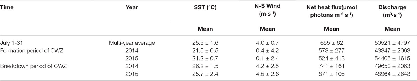
Table 2 Mean and standard deviations of SST, north-south wind speed (the positive value represented southerly wind speed), net heat flux at the center of CWZ (123.5°E, 32°N) in the YS, and the discharge at Datong station during July 1–31 of multi-year average and period of CWZ formation (July 1–17, 2014 and July 3–19, 2015) and breakdown periods (July 18–31, 2014 and July 20–31, 2015).
The variation characteristics of Changjiang river discharge anomalies during the formation periods of 2014 and 2015 were different (Figure 5E). The river discharge in the formation period of 2014 was slightly lower than the multi-year average discharge. However, it was higher in the formation period of 2015 (Table 2). From these simultaneous comparisons, SST anomalies, wind anomalies, and net heat flux anomalies showed temporal consistency, suggesting that surface wind and net heat flux during the summer of 2014 and 2015 could be two important physical factors for the formation of CWZs in the YS.
The three-dimensional physical-biogeochemical model (FVCOM-ERSEM) was used to investigate the formation mechanism of CWZ in the YS. Since observational data were more comprehensive for July of 2015 than that for 2014, the data of July 2015 was selected as a primary dataset for model verification. The model simulated physical and biogeochemical factors, including salinity, temperature, and concentration of DIN, DSi, DIP, TSM, and Chl-a, were quantitatively evaluated using Taylor diagrams (Figure 6). All simulated and observed data at 99 survey sites were normalized. The correlation coefficients of the simulated and observed salinity and temperature were >0.95 and ~0.8, respectively. The correlation coefficients of simulated and observed DIN and DSi were also ~0.95, and that of DIP was ~0.8. The correlation coefficient of simulated and observed Chl-a and TSM were both >0.5. The ratio of the standard deviation for simulated and observed salinity, temperature, nutrients, and Chl-a concentration was between 0.8 and 1.2; only the TSM was greater than1.5. Moreover, the root mean square difference (RMSD) of TSM was also greater than other parameters. Although the performances of Chl-a and TSM were slightly worse than the other factors, this model provided reasonable simulation for the physical and biogeochemical processes in the CRE and its adjacent waters during the summer of 2015.
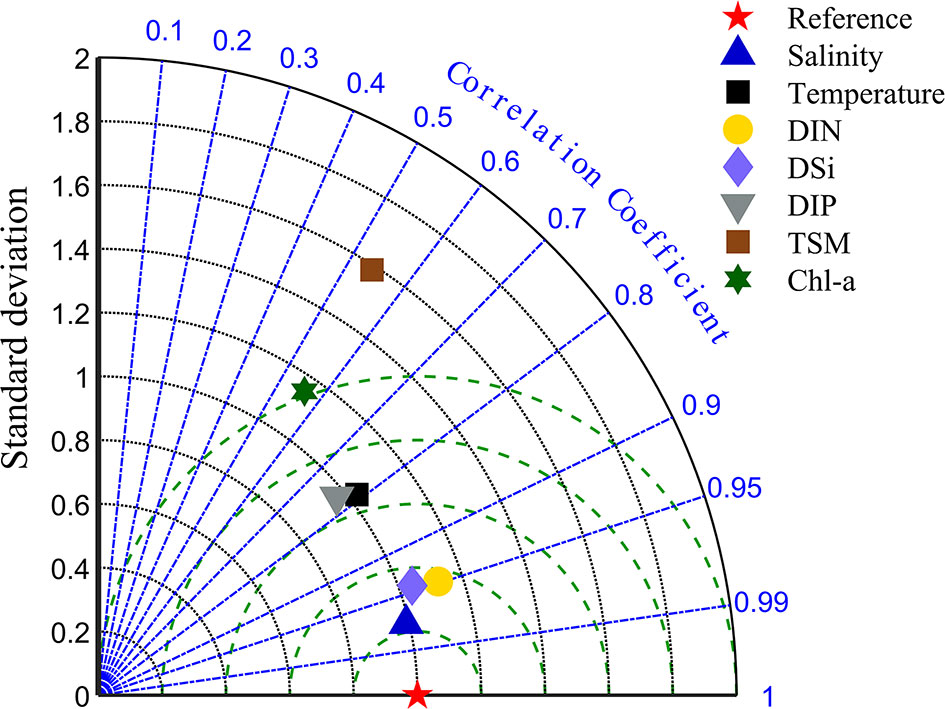
Figure 6 Taylor diagram of simulated and observed data for salinity, temperature, and concentration of DIN, DSi, DIP, TSM, and Chl-a in summer 2015. The radius distance represents the ratio of the standard deviation of the normalized modeling data to the standard deviation of the normalized observed data. Arc is the correlation coefficient between modeling data and observed data. Green dashed line is the ratio of root mean square difference (RMSD) between modeling data and observed data.
The spatial patterns of the model-simulated average SSS and SST in the formation period from July 3–19 (Figures 7A, B) were the same as the observed distributions (Figures 2C–F). We successfully captured the CWZ structure in the YS (Figure 7B). The plume front in the northeast region retreated west of 122.8°E and CWZ appeared off the plume front (Figures 7A, B). The VATKE in the CWZ was relatively high, with a range of 1−2×10⁻³m2·s−2 (Figure 7C). However, it was lower in the other deeper shelf water zone with a magnitude of<0.5×10⁻³m2·s−2. The potential energy anomaly (Ø) in the center of CWZ was extremely low (< 10 J·m3), suggesting that the CWZ was in a full vertical mixing state (Figure 7D). During the breakdown period, the plume front was significantly expended with a northeastward direction (Figure 7E). SST in the previous CWZ increased significantly, ranging from 24°C to 27°C, and the spatial SST gradient significantly decreased (Figure 7F). The VATKE decreased to approximately0.5×10−3m2·s−2 and the Ø increased to 20 J·m3–150 J·m3 in the previous CWZ, indicating the restoration of strong stratification (Figures 7G, H).
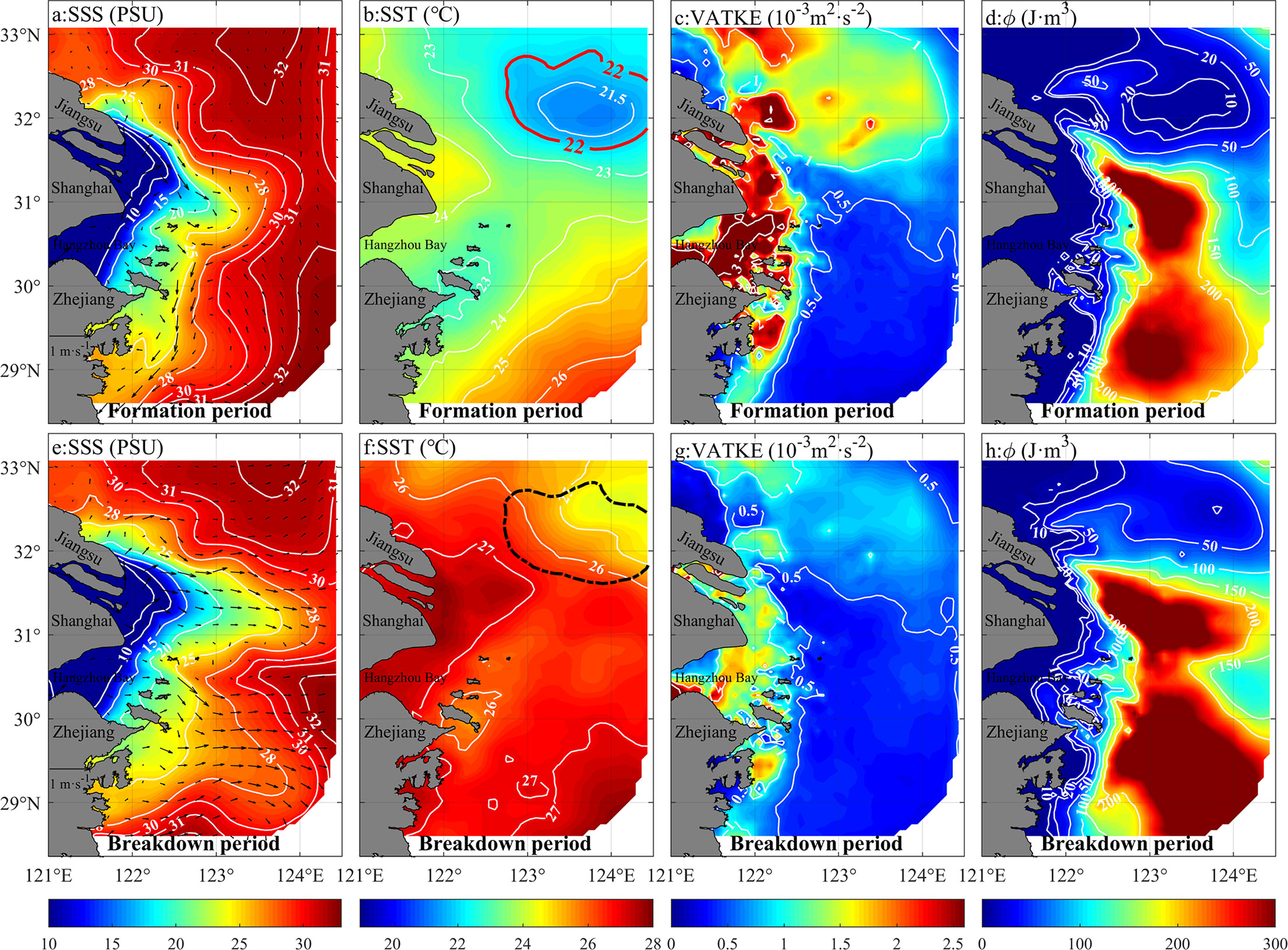
Figure 7 Spatial patterns of model-simulated average SSS (A, E) , SST (B, F), vertical-averaged turbulent kinetic energy (VATKE; C, G), and potential energy anomaly (Ø; D-H) during the formation period of July 3–19, 2015 (A-D) and breakdown period of July 20–31, 2015 (E-H). Black arrow in panels (A, E)represents surface flow, black dash line in panel (F) indicates the original CWZ.
A numerical model was used to further explore the influence of sea surface wind, net heating flux, and tidal mixing on the formation of the CWZ in the YS. Several model experiments were conducted to determine the individual effects of these physical factors. The control experiment (Case 1) considered the real surface wind, net heat flux, and tidal mixing in the summer of 2015. The wind forcing in Case 2 was changed to the climatological wind of June 30 to July 31 for years 2005–2018 to examine the wind effect. Similarly, the net heat flux in Case 3 was changed to the climatological condition, and Case 4 turned off the tidal forcing (more details about model configurations of numerical experiments, please see Table S1 in the Supplementary Material). All cases have the same other physical and biogeochemical forcing, such as initial field and riverine freshwater discharge.
The spatial distributions of the temporally averaged difference of SSS, SST, Ø, and VATKE during the formation period of July 3–19, 2015 among these experiments are shown in Figure 8. The difference in SSS between Case 1 and Case 2 in the CWZ was between −6 and −1, indicating that under the climatological wind forcing, the extension of the plume front toward offshore had increased significantly (Figure 8A). SST also increased by approximately 1°C–2°C; Ø increased by 10 J·m3–40 J·m3, whereas VATKE decreased in the CWZ (Figures 8B–D). These results indicated that the northerly wind in 2015 restrained the offshore extension of the plume front. However, the climatological southerly wind could favor an offshore extension into the YS and inhibit the formation of CWZs (Figures 8A–D).
Under the climatological net heat flux (Case 3), the SSS difference was very small, but SST increased by approximately 1.5°C in the whole study area, showing that the effect of net heat flux over this duration was spatially uniform (Figures 8E, F). Meanwhile, Ø only increased by 2 J·m3–8 J·m3, and VATKE slightly decreased in the CWZ in Case 3 (Figures 8G, H). The magnitudes of these differences are both much lower than those between Case 2 and Case 1. It suggests that the extraordinary northerly wind was the major dynamic factor attributed to the formation of CWZ in the YS, and the lower net heat flux was the secondary factor.
When removing the tide at the open boundary (Case 4), the circulation system was completely modified, showing a low-salinity plume extension around the Jiangsu coastal region (Figure 8I). Without tidal mixing, the SST rose by 3°C–4°C not only in the YS, but also in the whole inner shelf region; Ø increased by approximately 100 J·m3, and the VATKE reduced by 1.5×10⁻³m2·s−2 in the YS (Figures 8J–L). These differences indicated that offshore regions gained strong stratification in Case 4. It also suggests that wind-induced vertical mixing is much less than tidal mixing in this area. Tidal mixing is the most effective contributor to vertical mixing in the inner shelf (Figures 8I–L). After removing the tides, there was no CWZ occurrence, suggesting that strong tidal mixing is also a necessary physical factor for the formation of the CWZ.
Through these numerical experiments, we found that the formation and breakdown of CWZ was essentially determined due to status shifting between plume-induced stratification and tidal mixing (Figures 7, 8). This shift was primarily controlled by an extraordinary northerly wind, which was nearly the opposite of the prevailing summer monsoon. The low-salinity plume had a significant onshore retreat under this northerly wind, allowing the stratification status in CWZ to be relaxed and the tidal mixing to become dominant. The strong vertical mixing results in the SST declined, consequently forming the CWZ in the YS (Figure 3 ). The relatively lower net heat flux also encouraged this process. The breakdown of CWZ follows an opposite process. When the prevailing southerly monsoon was restored, the low-salinity plume has the northeastern extension and recovers the CWZ in the YS. The stratification intensity rapidly increased and inhibited the VATKE, resulting in the rapid dissipation of the CWZ.
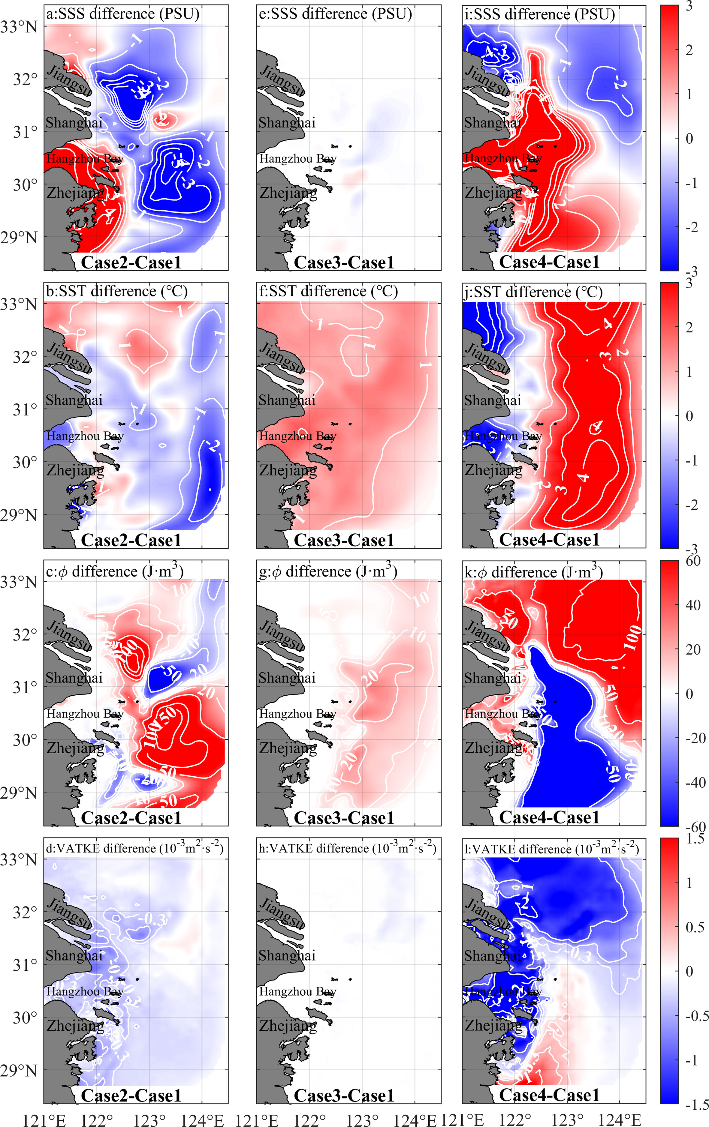
Figure 8 Spatial patterns of temporally averaged difference of SSS, SST, Ø, and VATKE between Case2 and Case1 (A–D), Case3 and Case1 (E–H), and Case4 and Case1(I–L) during the formation period of July 3–19, 2015.
In order to explore the effect of CWZ on the phytoplankton in the YS, the spatial distributions of mixed-layer depth (MLD) and Im are shown in Figure 9, demonstrating that the multi-year average MLD was 10–15 m off the plume front, and 5–10 m within the plume front (Figure 9A). However, during the summer of 2015, the MLD in the CWZ had a magnitude of 36.3±3.7 m (Figure 9B), which was deeper than the multi-year average (16.8±14.3 m). This was caused by strong vertical mixing in the CWZ. The multi-year average Im was >100 µmol photons m−2 s−1 in the YS (Figure 9C). But, the mean value of Im in the CWZ was only 29.7±8.5 µmol photons m−2 s−1 in the summer of 2015 (Figure 9 D and Table 3). But, the Imin the other shelf water zone was substantially high, reaching >150 µmol photons m−2 s−1. In the summer of 2015, the Im in the CWZ was not only less than the multi-year average value but also much less than that of surrounding waters.
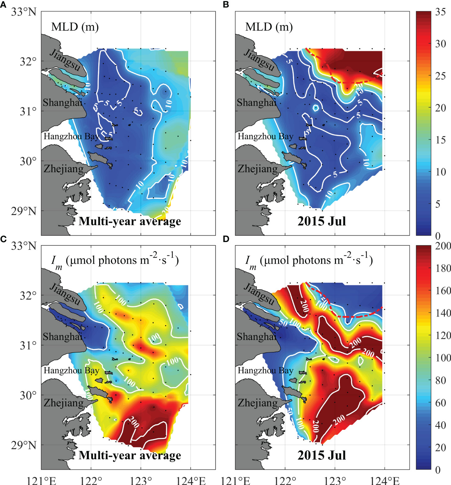
Figure 9 Spatial distributions of the mixed layer depth (MLD, A, B) and vertically averaged irradiance in the mixing layer (Im , C, D) of multi-year average (2013–2018) and 2015. The black line represents the plume front. The red line is the boundary of the CWZ.
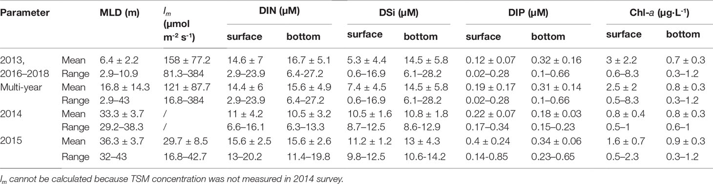
Table 3 Mean, standard deviations, and max-min ranges of the ecological variables in the CWZ during the summer of multi-year average, 2014 and 2015, based on surveys data.
The spatial distributions of DSi and DIP were similar; they gradually decreased with the extension of the low-salinity plume to offshore (Figures 10A–D and Figures S3A, B in the Supplementary Material). The nutrient concentration was lower in the shelf water off the plume front, with DSi and DIP concentrations less than 5 µM and 0.1 µM, respectively (Figures 10A, C). However, there was a relatively higher DIP concentration in the CWZ, with 0.4±0.24 µM in 2015, which were much higher than the average value of 0.12±0.07 µM of 2013 and 2016–2018 (Table 3). Meanwhile, the mean DIP concentration at the bottom of 2013 and 2016–2018 was approximately three times the surface DIP concentration. However, in the summer of 2014 and 2015, the nutrient concentrations of DSi, DIP and DIN in the surface and bottom layer of CWZ were very close due to strong vertical mixing in the CWZ.
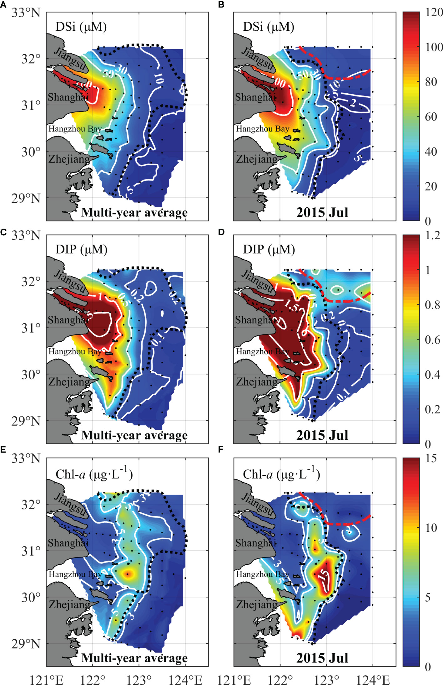
Figure 10 Spatial distributions of the dissolved silicate (DSi; A, B), dissolved inorganic phosphate (DIP; C, D), and Chl-a concentration (E, F) during the summer of multi-year average (2013–2018, A, C, E), and 2015 (B, D, F). The black line represents the plume front. The red line indicates the boundary of the CWZ.
A high Chl-a (defined as concentration of >5 µg·L−1) of the multi-year summer average mainly distributed in the landside of the plume front, and lower Chl-a concentration (<3 µg·L−1) were observed in the CRE and shelf water off the plume front (Figure 10 E). However, there was an isolated high Chl-a patch (>5 µg·L−1) off plume front, which appeared at the edge of CWZ in July, 2015 (Figure 10 F). The Chl-a concentration in the interior region of the CWZ was lower (Table 3). Therefore, the environmental factors and Chl-a during the formation of the CWZ had very different structures from that in multi-year non-CWZ conditions; this was caused by the status shift between plume-induced stratification and tide-induced vertical mixing.
Considering the CWZ event in 2015, for example, the FVCOM-ERESM model system was used to explore the temporal effect of the CWZ on Chl-a concentration. Figure 11 shows the temporal variation of environmental variables in the center of the CWZ in the YS. The simulated SSS was larger than 30 and remained stable during the formation period of the CWZ during July 3–19, 2015, and the Ø was less than 30 J·m3, suggesting that the local vertical mixing was intense (Figure 11A). During the period of July 3–12, the Ø was less than 10 J·m3, indicating that the water column was fully mixed. In the breakdown period of CWZ during July 20–31, when the low-salinity plume gradually restored its coverage over the original CWZ, the SSS decreased rapidly and Ø increased dramatically from 30 to 100 J·m3, suggesting that stratification restored its dominance.
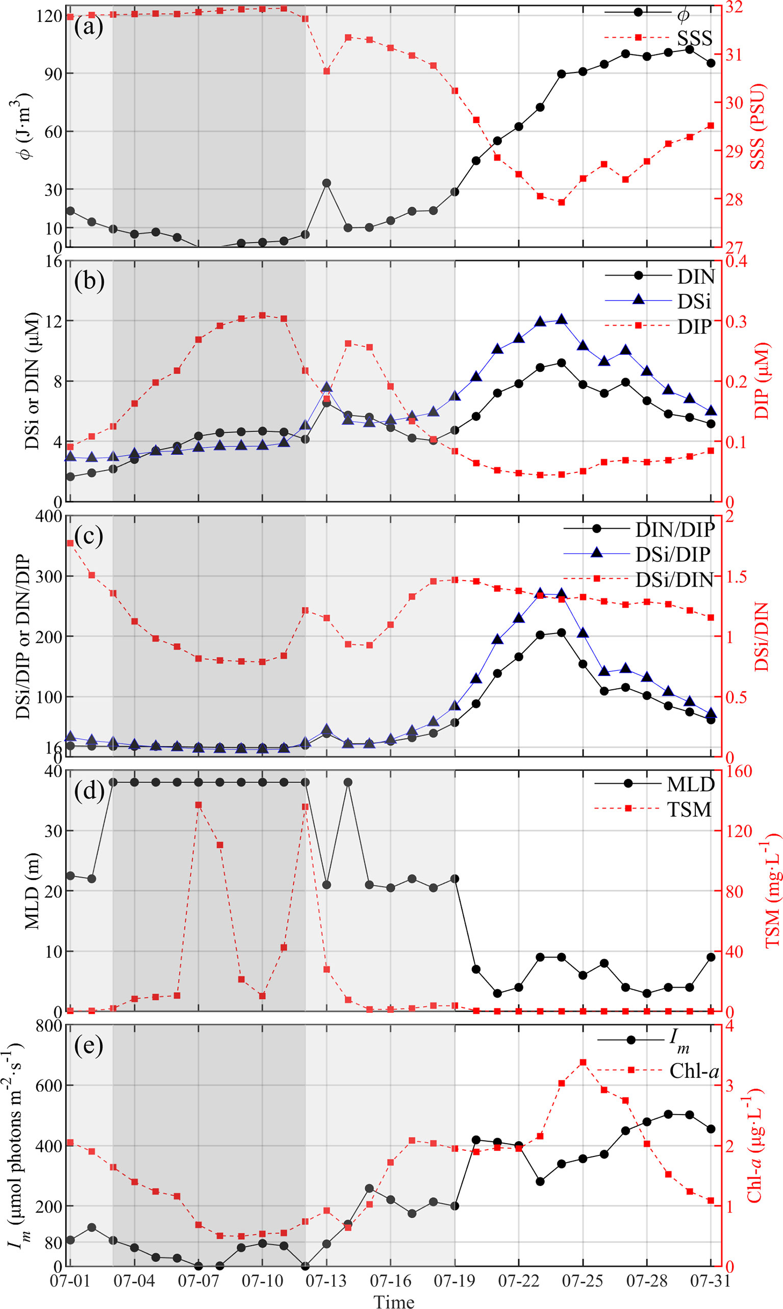
Figure 11 Temporal variation of simulated physical and ecological variables at the center of CWZ during July 1–31, 2015. (A) Ø and SSS; (B) surface nutrient concentrations; (C) Surface nutrient ratio; (D) MLD and surface total suspended matter (TSM); (E)Im and surface Chl-a concentration. The state of water mixing and stratification is indicated by dark gray, light gray, and white, deep grey shaded period represents that the water column is fully mixed.
Under strong vertical mixing during July 1–12, the surface nutrient concentration also demonstrated a continuous increase; in particular, DIP concentration increased significantly from 0.1 µM to 0.3 µM (Figure 11B). Meanwhile, the nutrient ratio was close to the Redfield ratio (Si:N:P=16:16:1; Redfield, 1958) (Figure 11C). However, during the breakdown period of July 20–31, the DSi/DIP and DIN/DIP were both larger than 60. This indicated there was heavy relative DIP limitation, of which the threshold was DSi/DIP >22 and DIN/DIP >22 (Justić et al., 1995). Because the surface shelf water was usually oligotrophic with severe P-limitation under the existence of stratification, the bottom layer contained rich nutrients (Li et al., 2021; Tian et al., 1993; Tseng et al., 2014). The intense mixing in the CWZ transported nutrient-rich water from the bottom to surface column, and significantly relaxed the P-limitation (Figures 11B, C). Under the re-coverage of the low-salinity plume during the breakdown period of July 20–31, 2015, the concentration of DIN and DSi increased rapidly, followed by a noticeable decrease after reaching the peak on July 24. However, the DIP concentration was maintained at the lower level of 0.05–0.1 µM. This indicates that the relative P-limitation was significant in the low-salinity plume and stratification restrained the nutrients transport from the bottom to the surface layer. Thus, when the surface DIP was consumed, the P-limitation feature would reappear.
Under the full vertical mixing condition from July 3–12, the MLD increased in depth (reaching 38 m consistent with the water depth here) and remained stable, and the TSM concentration also increased from<2 mg·L−1 to a maximum of 140 mg·L−1 (Figure 11D). Mixing-induced sediment resuspension in the CWZ resulted in high TSM concentrations in the water column. As stratification gradually developed after the CWZ breakdown, it could inhibit the resuspension of sediment. The MLD and TSM both decreased; MLD was<10 m and TSM was restored to its low level of<1 mg·L−1 from July 20-31.
The intensity Im decreased to<80 µmol photons m−2 s−1, influenced by the high TSM and MLD during the period of July 3–13 (Figure 11E). With the decrease of MLD and TSM, the intensity Im gradually increased and maintained a high level of >300 µmol photons m−2s−1 during the July 20–31 period. The Chl-a concentration showed a similar variation as Im during the formation period of the CWZ (Figure 11E). It was first reduced to approximately 0.5 µg·L−1 during the period of July 3–12, and then gradually increased to a maximum of 3.5 µg·L−1 on July 25, and then decreased rapidly to 1 µg·L−1 due to the P-limitation.
Under the strong mixing condition in the CWZ formation period, the nutrient concentrations were all higher than the thresholds of absolute nutrient limitation, which were DIP >0.1 µM, DIN >1 µM, DSi >2 µM according to previous studies (Rhee, 1973; Harrison et al., 1977; Goldman and Glibert, 1983; Nelson and Brzezinski, 1990; Justić et al., 1995). However, during the fully-mixed period, the Im was lower than the light-limitation threshold (Im<80 µmol photons m−2s−1) in the shelf water zone (Hitchcock and Smayda, 1977; Kirk, 1994; Thompson, 1999; Lin et al., 2019). Therefore, it could be inferred that weak light limited the growth of phytoplankton and caused the lowest Chl-a concentration between July 3–12. In the early stage of the plume extension on July 20–25, light is sufficient. With adequate nutrient levels in the upper layer during the formation period, phytoplankton could grow rapidly, and Chl-a concentration reached its maximum (Figure 11E). However, when the surface nutrients, particularly DIP, were consumed, the P-limitation was reinstated and led to the reduction of Chl-a during July 25–31.
The formation and breakdown mechanism of CWZ in the YS is summarized in the schematic diagram (Figure 12). Because the density of the Changjiang plume with low salinity and high SST is much lower than that of the shelf water, strong stratification dominates within the plume front. In the CRE and its adjacent water, the northerly wind produces onshore Ekman transport, causing the plume front to retreat to the nearshore region and the stratification weakened in the YS (Figure 12A). When tide-induced mixing becomes the dominant physical factor and transports the low-temperature water from the bottom to the surface, the CWZ forms in the YS. Thus, the plume front is consistent with the western boundary of the CWZ. In addition, under the relatively low heat flux, the surface heating effect is difficult to form thermal stratification in the YS under strong tidal mixing. With the increase of water depth in the offshore direction, the intensity of tidal mixing gradually decreases. The VATKE in the area deeper the 50 m is relatively lower (Figures 7C, G). The thermal stratification could appear in deeper regions due to the surface heating (Figure 12A).
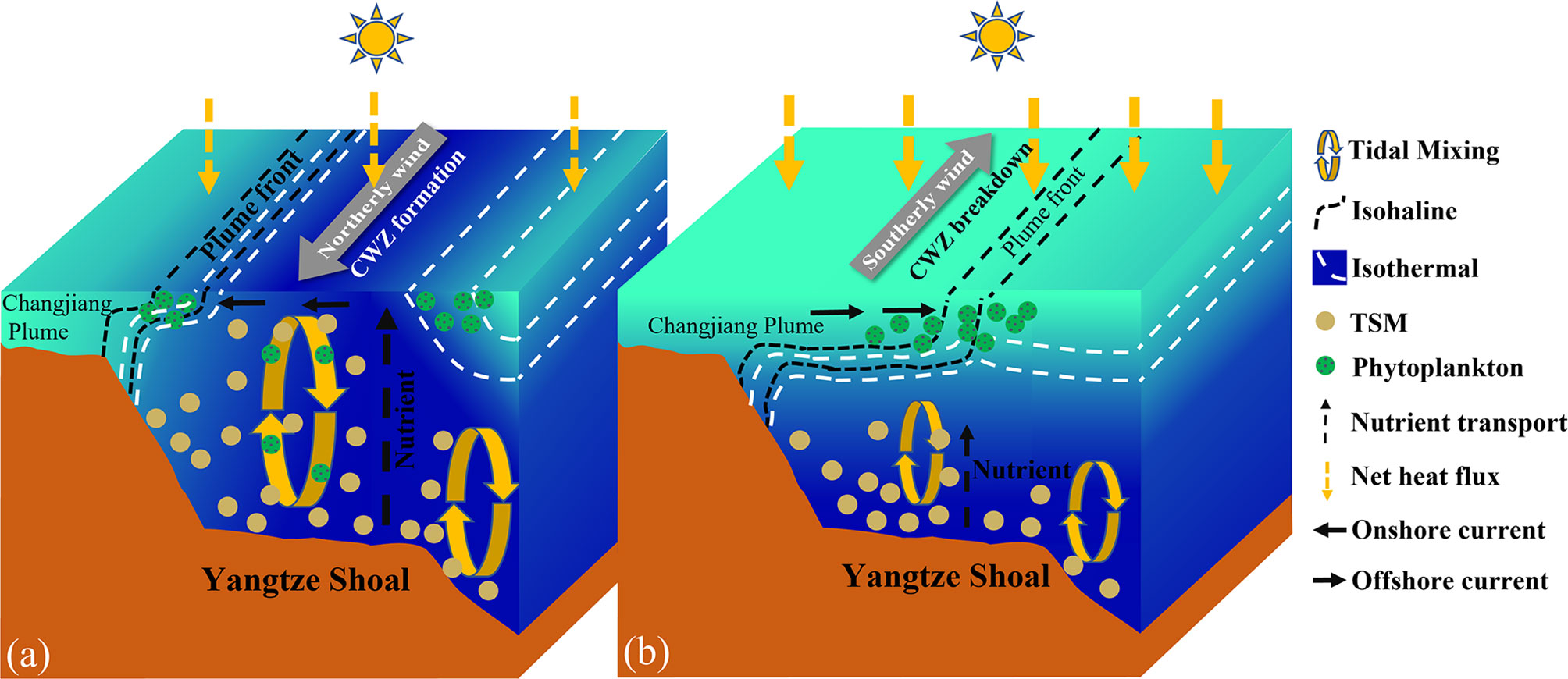
Figure 12 Schematic diagram of the formation (A) and breakdown (B) mechanism of the CWZ in the YS and its effect on the phytoplankton growth.
The breakdown of the CWZ is caused by the restoration of southerly wind, driving the plume offshore extension and then recovering the YS (Figure 12B). Therefore, the dominant factors in YS rapidly shift from tidal mixing to stratification, resulting in the increase of SST. The prevailing southerly summer monsoon leads to the low frequency of the CWZ formation in the YS (Figure 5 ). Thus, the climatological monthly SST image cannot capture the CWZ in the YS (Lü et al., 2010; Ren et al., 2014).
Various summer CWZs were found around the Jiangsu and Korean coastal regions and east of Zhoushan Island in previous studies (Zhu, 2003; Lü et al., 2010; Ren et al., 2014). However, these CWZs were generated by a different physical mechanism. For example, the CWZ around Zhoushan Island was produced by persistent upwelling (Figures 2D, 4). The CWZs in Jiangsu coastal region and the Korean coastal region were related to the thermal TMF and tide-induced upwelling (Lü et al., 2010; Ren et al., 2014). The position of TMF can be determined by the parameterization h/u3 (Simpson and Hunter, 1974; Simpson et al., 1978). Thus, CWZs related to the TMF mainly appeared in the nearshore area with huge water depth variations (Ren et al., 2014; Huang et al., 2018). This type of CWZ also appeared in the summer on the coast of the Shandong Peninsula (Huang et al., 2018), western Kamchatka shelf (Zhabin et al., 2019), and western Iris sea (Simpson and Hunter, 1974).
This work explored a different formation/breakdown mechanism of CWZs in the YS under the interaction of extraordinary wind, astronomical tide and the Changjiang River plume. Many large estuaries have extensive plume affected areas, which are greatly influenced by wind fields (e.g., the Amazon, Mississippi, Changjiang, Pearl, and Rio de la Plata river plumes, etc. (Beardsley et al., 1985; Lentz and Limeburner, 1995; Pimenta et al., 2005; Schiller et al., 2011; Pan et al., 2014). The other estuaries also have a similar formation process to the CWZ in the YS. For example, in the Rio de la Plata estuary and its adjacent shelf, the weak but longer upwelling-favorable wind could drive the Rio de la Plata River plume to offshore regions, weakening the nearshore stratification and increasing upwelling at the surface to form a CWZ (Pimenta et al., 2008). However, the offshore transport of the Rio de la Plata River plume is driven by more intense but short-lasting upwelling-favorable wind could be interrupted by the subsequent downwelling favorable wind. Thus, the upwelling was confined and could not form a stable surface CWZ (Pimenta et al., 2008).
The shift between stratification and mixing in CWZs could alter the light and nutrient conditions influencing the Chl-a concentration variations (Cloern, 1999; Sun and Cho, 2010; Wei et al., 2016). First, tidal mixing could transport the bottom-rich nutrients to the upper water column (Figure 12A), which was beneficial to the growth of phytoplankton at the sea surface (Sun and Cho, 2010; Wei et al., 2016). However, phytoplankton were moved vertically along with the mixing water. If the euphotic layer was constant, the MLD was deeper, and phytoplankton stayed in the dark area below the euphotic layer for a longer period, which reduced the underwater light usage of phytoplankton (Cloern, 1996; Lin et al., 2019). Vertical mixing also promotes the sediment resuspension, which increases the attenuation coefficient of the underwater beam and the euphotic layer shallows. Thus, there were many estuaries and coastal areas with high nutrient concentrations, but light limitation resulted in lower Chl-a concentration, as is the case of the CRE (Wang et al., 2019; Li et al., 2021), Pearl River Estuary (Harrison et al., 2008), springtime TMF in the Jiangsu coastal region (Wei et al., 2016), Benguela upwelling region (Burger et al., 2020) and the center CWZ in the YS (Figures 11, 12A).
When stratification gradually increased after the strong vertical mixing or active upwelling, the Chl-a concentrations tended to rise at first due to improved lighting conditions and sufficient nutrients, such as the spring algal blooms in the Yellow Sea (Wei et al., 2016), the Benguela upwelling relaxation period (Burger et al., 2020) and the early period of CWZ breakdown (July 20–25, Figure 11). Stratification also led to the congregation of phytoplankton in the upper layers, causing the surface Chl-a concentration to increase (Figure 12). Since the CWZ stratified firstly near the edge, then the central region (Figure 4), the high Chl-a patch firstly appeared at the edge of the CWZ in 2014 and 2015 (Figure 10F and Figure S3C), where its concentrations were usually lower in previous surveys (Guo et al., 2014; Tseng et al., 2014; Wang et al., 2019). However, stratification caused by both surface heating and low-salinity plumes would inhibit the vertical transport of nutrients from the bottom to the surface and might have resulted in a nutrient limitation in the surface layer, especially after the nutrient consumption by phytoplankton growth.
In this study, we identified a synoptic CWZ formation in the YS off the CRE through comprehensive field surveys during the summers of 2014 and 2015. The mean SST in the CWZ was approximately 4°C lower than the multi-year average. The physical-biogeochemical coupling model system was applied to examine the driving mechanism and its effects on environmental factors and Chl-a concentration during the formation and breakdown periods of the CWZ. Through observational and modeling results, the formation and breakdown of the CWZ were primarily determined by the change in the prevailing wind direction, followed by the secondary effect from the weaker net heat flux. The extraordinary northerly wind during July 1–17, 2014, and July 3–19, 2015, which flowed in the opposite direction of the prevailing monsoon, produced the onshore retreat of the low-salinity plume. Tidal mixing became the dominant physical factor off the plume front, resulting in higher VATKE and TSM concentrations, as well as greater MLD in the CWZ. The strong mixing in the CWZ increased the surface DIP concentration and relaxed the P-limitation. However, it also caused light limitation due to higher TSM and deeper MLD; Chl-a concentration was lower in the center of CWZ. After the wind direction was restored, the low-salinity plume re-covered the CWZ, and phytoplankton experienced a fast growth until surface nutrients were depleted and the nutrient limitation appeared. Patches of high Chl-a concentration occurred at the edge of the CWZ. This article has important implications for exploring the formation mechanisms of CWZs under the physical interaction of atmospheric wind and the low-salinity plume and its impact on phytoplankton dynamics.
The datasets presented in this study can be found in online repositories. The names of the repository/repositories and accession number(s) can be found below: https://doi.org/10.5281/zenodo.6469302.
WL, JG, PD, and DL conceived the study; WL, XZ, and JG provided the observational data and modeling data; WL analyzed the dataset and performed relevant calculations; WL wrote the manuscript under the guidance of JG, PD, and DL; WL and JG revised the manuscript. All authors contributed to and approved the manuscript.
This research is supported by the National Natural Science Foundation of China (Grant No. 41776104, 41606025, 41876127 and 42030402) and the Research Project of China Three Gorges Corporation (Grant No. 202103552).
The authors declare that the research was conducted in the absence of any commercial or financial relationships that could be construed as a potential conflict of interest.
All claims expressed in this article are solely those of the authors and do not necessarily represent those of their affiliated organizations, or those of the publisher, the editors and the reviewers. Any product that may be evaluated in this article, or claim that may be made by its manufacturer, is not guaranteed or endorsed by the publisher.
Thanks to all the researchers and crews who participated in the Changjiang River Estuary Shared Surveys Project (Grant No. 41649903, 41549903, 41449903, and 41349903).
The Supplementary Material for this article can be found online at: https://www.frontiersin.org/articles/10.3389/fmars.2022.926738/full#supplementary-material
Beardsley R. C., Limeburner R., Yu H., Cannon G. A. (1985). Discharge of the Changjiang (Yangtze River) Into the East China Sea. Continental. Shelf. Res. 4, 57–76. doi: 10.1016/0278-4343(85)90022-6
Bowers D. G., Lwiza K. (1994). The Temperature Minimum at Tidal Fronts. Annales. Geophysicae. 12, 683–687. doi: 10.1007/s00585-994-0683-2
Bruggeman J., Bolding K. (2014). A General Framework for Aquatic Biogeochemical Models. Environ. Model. Software. 61, 249–265. doi: 10.1016/j.envsoft.2014.04.002
Burger J. M., Moloney C. L., Walker D. R., Parrott R. G., Fawcett S. E. (2020). Drivers of Short-Term Variability in Phytoplankton Production in an Embayment of the Southern Benguela Upwelling System. J. Mar. Syst. 208, 103341. doi: 10.1016/j.jmarsys.2020.103341
Butenschön M., Clark J., Aldridge J. N., Allen J. I., Artioli Y., Blackford J., et al. (2016). ERSEM 15.06: A Generic Model for Marine Biogeochemistry and the Ecosystem Dynamics of the Lower Trophic Levels. Geoscientific. Model. Dev. 9, 1293–1339. doi: 10.5194/gmd-9-1293-2016
Chang P., Isobe A. (2003). A Numerical Study on the Changjiang Diluted Water in the Yellow and East China Seas. J. Geophysical. Research.: Oceans. 108:C93299. doi:10.1029/2002JC001749
Chen J., Li D., Chen B., Hu F., Zhu H., Liu C. (1999). The Processes of Dynamic Sedimentation in the Changjiang Estuary. J. Sea. Res. 41, 129–140. doi: 10.1016/S1385-1101(98)00047-1
Chen C., Liu H., Beardsley R. C. (2003). An Unstructured Grid, Finite-Volume, Three-Dimensional, Primitive Equations Ocean Model: Application to Coastal Ocean and Estuaries. J. Atmospheric. Oceanic. Technol. 20, 159–186. doi: 10.1175/1520-0426(2003)020<0159:AUGFVT>2.0.CO;2
Chu P. C., Fan C. (2011). Maximum Angle Method for Determining Mixed Layer Depth From Seaglider Data. J. Oceanography. 67, 219–230. doi: 10.1007/s10872-011-0019-2
Cloern J. E. (1987). Turbidity as a Control on Phytoplankton Biomass and Productivity in Estuaries. Continental. Shelf. Res. 7, 1367–1381. doi: 10.1016/0278-4343(87)90042-2
Cloern J. E. (1996). Phytoplankton Bloom Dynamics in Coastal Ecosystems: A Review With Some General Lessons From Sustained Investigation of San Francisco Bay, California. Rev. Geophysics. 34, 127–168. doi: 10.1029/96RG00986
Cloern J. E. (1999). The Relative Importance of Light and Nutrient Limitation of Phytoplankton Growth: A Simple Index of Coastal Ecosystem Sensitivity to Nutrient Enrichment. Aquat. Ecol. 33, 3–15. doi: 10.1023/A:1009952125558
Cloern J. E., Jassby A. D., Schraga T. S., Nejad E., Martin C. (2017). Ecosystem Variability Along the Estuarine Salinity Gradient: Examples From Long-Term Study of San Francisco Bay. Limnology. Oceanography. 62, S272–S291. doi: 10.1002/lno.10537
de Boer G. J., Pietrzak J. D., Winterwerp J. C. (2009). SST Observations of Upwelling Induced by Tidal Straining in the Rhine ROFI. Continental. Shelf. Res. 29, 263–277. doi: 10.1016/j.csr.2007.06.011
Egbert G. D., Erofeeva S. Y. (2002). Efficient Inverse Modeling of Barotropic Ocean Tides. J. Atmospheric. Oceanic. Technol. 19, 183–204. doi: 10.1175/1520-0426(2002)019<0183:EIMOBO>2.0.CO;2
Gao L., Li D., Ishizaka J., Zhang Y., Zong H., Guo L. (2015). Nutrient Dynamics Across the River-Sea Interface in the Changjiang (Yangtze River) Estuary–East China Sea Region. Limnology. Oceanography. 60, 2207–2221. doi: 10.1002/lno.10196
Ge J., Ding P., Chen C., Hu S., Fu G., Wu L. (2013). An Integrated East China Sea–Changjiang Estuary Model System With Aim at Resolving Multi-Scale Regional–Shelf–Estuarine Dynamics. Ocean. Dynamics. 63, 881–900. doi: 10.1007/s10236-013-0631-3
Ge J., Torres R., Chen C., Liu J., Xu Y., Bellerby R., et al. (2020a). Influence of Suspended Sediment Front on Nutrients and Phytoplankton Dynamics Off the Changjiang Estuary: A FVCOM-ERSEM Coupled Model Experiment. J. Mar. Syst. 204, 103292. doi: 10.1016/j.jmarsys.2019.103292
Ge J., Shi S., Liu J., Xu Y., Chen C., Bellerby R., et al. (2020b). Interannual Variabilities of Nutrients and Phytoplankton Off the Changjiang Estuary in Response to Changing River Inputs. J. Geophysical. Research.: Oceans. 125 :e2019JC015595. doi: 10.1029/2019JC015595
Geyer W. R. (1993). The Importance of Suppression of Turbulence by Stratification on the Estuarine Turbidity Maximum. Estuaries 16, 113–125. doi: 10.2307/1352769
Goldman J., Glibert P. (1983). “Kinetics of Inorganic Nitrogen Uptake by Phytoplankton”, in Nitrogen in the Marine Environment. Eds. Caroebter E. J., Capone D. C. (New York: Academic Press), 233–274.
Guo S., Feng Y., Wang L., Dai M., Liu Z., Bai Y., et al. (2014). Seasonal Variation in the Phytoplankton Community of a Continental-Shelf Sea: The East China Sea. Mar. Ecol. Prog. Ser. 516, 103–126. doi: 10.3354/meps10952
Harrison P. J., Conway H. L., Holmes R. W., Davis C. O. (1977). Marine Diatoms Grown in Chemostats Under Silicate or Ammonium Limitation. III. Cellular Chemical Composition and Morphology of Chaetoceros Debilis, Skeletonema Costatum, and Thalassiosira Gravida. Mar. Biol. 43, 19–31. doi: 10.1007/BF00392568
Harrison P. J., Yin K., Lee J. H. W., Gan J., Liu H. (2008). Physical–biological Coupling in the Pearl River Estuary. Continental. Shelf. Res. 28, 1405–1415. doi: 10.1016/j.csr.2007.02.011
He Y., Deng R., Chen Q., Chen L., Qin Y. (2011). Diffuse Attenuation Coefficient of Suspended Sediment Based on ASD Spectrometer. Acta Scientiarum. Naturalium. Universitatis. Sunyatseni. (in Chinese) 50, 134–140. 0529-6579(2011) 03-0134-07
Hitchcock G. L., Smayda T. J. (1977). The Importance of Light in the Initiation of the 1972-1973 Winter-Spring Diatom Bloom in Narragansett Bay1. Limnology. Oceanography. 22, 126–131. doi: 10.4319/lo.1977.22.1.0126
Huang M., Liang X. S., Wu H., Wang Y. (2018). Different Generating Mechanisms for the Summer Surface Cold Patches in the Yellow Sea. Atmosphere-Ocean 56, 199–211. doi: 10.1080/07055900.2017.1371580
Hu F., Hu H., Gu G., Su C., Gu X. (1995). Salinity Front in the Changjiang River Estuary. Oceanologia. Et Limnologia. Sin. (in Chinese) 26, 23–31. doi:10.3321/j.issn:0029-814X.1995.z1.004
Justić D., Rabalais N. N., Turner R. E., Dortch Q. (1995). Changes in Nutrient Structure of River-Dominated Coastal Waters: Stoichiometric Nutrient Balance and its Consequences. Estuarine. Coast. Shelf. Sci. 40, 339–356. doi: 10.1016/S0272-7714(05)80014-9
Kirk J. T. O. (1994). Light and Photosynthesis in Aquatic Ecosystems. 2rd ed (New York: Cambridge University Press).
Lentz S. J., Limeburner R. (1995). The Amazon River Plume During AMASSEDS: Spatial Characteristics and Salinity Variability. J. Geophysical. Research.: Oceans. 100, 2355–2375. doi: 10.1029/94JC01411
Li W., Ge J., Ding P., Ma J., Glibert P. M., Liu D. (2021). Effects of Dual Fronts on the Spatial Pattern of Chlorophyll-A Concentrations in and Off the Changjiang River Estuary. Estuaries. Coasts. 44, 1408–1418. doi: 10.1007/s12237-020-00893-z
Lin L., Wang Y., Liu D. (2019). Vertical Average Irradiance Shapes the Spatial Pattern of Winter Chlorophyll-a in the Yellow Sea. Estuarine. Coast. Shelf. Sci. 224, 11–19. doi: 10.1016/j.ecss.2019.04.042
Liu B.C, Feng L.C., and . (2012). An Observational Analysis of the Relationship Between Wind and the Expansion of the Changjiang River Diluted Water during Summer. Atmospheric and Oceanic Science Letters 5: 384-388. doi:10.1080/16742834.2012.11447027
Lohrenz S. E., Fahnenstiel G. L., Redalje D. G., Lang G. A., Dagg M. J., Whitledge T. E., et al. (1999). Nutrients, Irradiance, and Mixing as Factors Regulating Primary Production in Coastal Waters Impacted by the Mississippi River Plume. Continental. Shelf. Res. 19, 1113–1141. doi: 10.1016/S0278-4343(99)00012-6
Lü X., Qiao F., Xia C., Wang G., Yuan Y. (2010). Upwelling and Surface Cold Patches in the Yellow Sea in Summer: Effects of Tidal Mixing on the Vertical Circulation. Continental. Shelf. Res. 30, 620–632. doi: 10.1016/j.csr.2009.09.002
Lü X., Qiao F., Xia C., Zhu J., Yuan Y. (2006). Upwelling Off Yangtze River Estuary in Summer. J. Geophysical. Res. 111. C11S08. doi: 10.1029/2005JC003250
Nelson D. M., Brzezinski M. A. (1990). Kinetics of Silicic Acid Uptake by Natural Diatom Assemblages in Two Gulf Stream Warm-Core Rings. Mar. Ecology-Progress. Ser. 62, 283–292. doi: 10.3354/meps062283
Pan J., Gu Y., Wang D. (2014). Observations and Numerical Modeling of the Pearl River Plume in Summer Season. J. Geophysical. Research.: Oceans. 119, 2480–2500. doi: 10.1002/2013JC009042
Pimenta F. M., Campos E. J. D., Miller J. L., Piola A. R. (2005). A Numerical Study of the Plata River Plume Along the Southeastern South American Continental Shelf. Braz. J. Oceanography. 53, 129–146. doi: 10.1590/S1679-87592005000200004
Pimenta F. M., Garvine R. W., Münchow A. (2008). Observations of Coastal Upwelling Off Uruguay Downshelf of the Plata Estuary, South America. J. Mar. Res. 66, 835–872. doi: 10.1357/002224008788064577
Prasanna Kumar S., Muraleedharan P. M., Prasad T. G., Gauns M., Ramaiah N., De Souza S. N., et al. (2002). Why Is the Bay of Bengal Less Productive During Summer Monsoon Compared to the Arabian Sea? Geophysical. Res. Lett. 29, 81–88. doi: 10.1029/2002GL016013
Redfield A. C. (1958). The Biological Control of Chemical Factors in the Environment. Am. Scientist. 46, 221A–230A. https://www.jstor.org/stable/27827150
Ren S., Xie J., Zhu J. (2014). The Roles of Different Mechanisms Related to the Tide-Induced Fronts in the Yellow Sea in Summer. Adv. Atmospheric. Sci. 31, 1079–1089. doi: 10.1007/s00376-014-3236-y
Rhee G. Y. (1973). A Continuous Culture Study of Phosphate Uptake, Growth Rate and Polyphosphate in Scenedesmus Sp. J. Phycology. 9, 495–506. doi: 10.1111/j.1529-8817.1973.tb04126.x
Riley G. A. (1957). Phytoplankton of the North Central Sargasso Sea 1950-52. Limnology. Oceanography. 2, 252–270. doi: 10.1002/lno.1957.2.3.0252
Sapozhnikov V. V., Ivanova O. S., Mordasova N. V. (2011). Identification of Local Upwelling Zones in the Bering Sea Using Hydrochemical Parameters. Oceanology 51, 247. doi: 10.1134/S0001437011020135
Schiller R. V., Kourafalou V. H., Hogan P., Walker N. D. (2011). The Dynamics of the Mississippi River Plume: Impact of Topography, Wind and Offshore Forcing on the Fate of Plume Waters. J. Geophysical. Research.: Oceans. 116, C06029. doi: 10.1029/2010JC006883
Scully M. E., Geyer W. R. (2012). The Role of Advection, Straining, and Mixing on the Tidal Variability of Estuarine Stratification. J. Phys. Oceanography. 42, 855–868. doi: 10.1175/JPO-D-10-05010.1
Simpson J., Allen C., Morris N. (1978). Fronts on the Continental Shelf. J. Geophysical. Res. 83, 4607–4614. doi: 10.1029/JC083iC09p04607
Simpson J. H., Crisp D. J., Hearn C. (1981). The Shelf-Sea Fronts: Implications of Their Existence and Behaviour. Philos. Trans. R. Soc.: Mathematical. Phys. Eng. Sci. 302, 531–546. http://www.jstor.org/stable/37036
Simpson J. H., Sharples J., Rippeth T. P. (1991). A Prescriptive Model of Stratification Induced by Freshwater Runoff. Estuar. Coast. Shelf. Sci. 33, 23–35. doi: 10.1016/0272-7714(91)90068-M
Smith W. O., Demaster D. J. (1996). Phytoplankton Biomass and Productivity in the Amazon River Plume: Correlation With Seasonal River Discharge. Continental. Shelf. Res. 16, 291–319. doi: 10.1016/0278-4343(95)00007-N
Sousa F. M., Nascimento S., Casimiro H., Boutov D. (2008). Identification of Upwelling Areas on Sea Surface Temperature Images Using Fuzzy Clustering. Remote Sens. Environ. 112, 2817–2823. doi: 10.1016/j.rse.2008.01.014
Sun Y. J., Cho Y. K. (2010). Tidal Front and its Relation to the Biological Process in Coastal Water. Ocean. Sci. J. 45, 243–251. doi: 10.1007/s12601-010-0022-3
Thompson P. (1999). The Response of Growth and Biochemical Composition to Variations in Daylength, Temperature and Irradiance in the Marine Diatom Thalassiosira Pseudonana (Bacillariophyceae). J. Phycology. 35, 1215–1223. doi: 10.1046/j.1529-8817.1999.3561215.x
Tseng Y. F., Lin J., Dai M., Kao S. J. (2014). Joint Effect of Freshwater Plume and Coastal Upwelling on Phytoplankton Growth Off the Changjiang River. Biogeosciences 11, 409–423. doi: 10.5194/bg-11-409-2014
Wang Y., Wu H., Gao L., Shen F., Liang X. S. (2019). Spatial Distribution and Physical Controls of the Spring Algal Blooming Off the Changjiang River Estuary. Estuaries. Coasts. 42, 1066–1083. doi: 10.1007/s12237-019-00545-x
Wei Q., Li X., Wang B., Fu M., Ge R., Yu Z. (2016). Seasonally Chemical Hydrology and Ecological Responses in Frontal Zone of the Central Southern Yellow Sea. J. Sea. Res. 112, 1–12. doi: 10.1016/j.seares.2016.02.004
Zhabin I. A., Vanin N. S., Dmitrieva E. V. (2019). Summer Wind-Driven Upwelling and Tidal Mixing on the Western Kamchatka Shelf in the Sea of Okhotsk. Russian Meteorology. Hydrology. 44, 130–135. doi: 10.3103/S1068373919020067
Zhang Y., Qin B., Chen W., Gao G., Chen Y. (2004). Experimental Study on Underwater Light Intensity and Primary Productivity Caused by Variation of Total Suspended Matter. Adv. Water Sci. (in Chinese), 15. 615–620. doi: 10. 13984 /j. cnki.cn37-1141. 2003. 02. 005
Zhang Y., Qin B., Chen W., Yang D., Ji J. (2003). Analysis on Distribution and Variation of Beam Attenuation Coefficient of Taihu Lake’ s Water. Adv. Water Sci. (in Chinese), 14. 347–353. doi: 10. 13984 /j. cnki.cn37-1141. 2003. 02. 005
Zhang Z., Zhou M., Zhong Y., Zhang G., Jiang S., Gao Y., et al. (2020). Spatial Variations of Phytoplankton Biomass Controlled by River Plume Dynamics Over the Lower Changjiang Estuary and Adjacent Shelf Based on High-Resolution Observations. Front. Mar. Sci. 7. doi: 10.3389/fmars.2020.587539
Zhao L., Guo X. (2011). Influence of Cross-Shelf Water Transport on Nutrients and Phytoplankton in the East China Sea: A Model Study. Ocean. Sci. 7, 27–43. doi: 10.5194/os-7-27-2011
Zhu J. (2003). Dynamic Mechanism of the Upwelling on the West Side of the Submerged River Valley Off the Changjiang Mouth in Summertime. Chin. Sci. Bull. 48, 2754–2758. doi: 10.1007/BF02901770
Zhu W., Jiang Y., Zhao L., Tian T. (2010). Field Survey and Analysis of Influence of Suspended Sediment on Algae Growth. Adv. Water Sci. (in Chinese) 21, 241–247. doi: 10.14042/j.cnki.32.1309.2010.02.015
Keywords: cold-water zone, estuarine plume, tidal mixing, physical-biogeochemical coupling model, light-limitation, nutrient, phytoplankton
Citation: Li W, Zhou X, Ge J, Ding P and Liu D (2022) Formation and Breakdown of an Offshore Summer Cold-Water Zone and Its Effect on Phytoplankton. Front. Mar. Sci. 9:926738. doi: 10.3389/fmars.2022.926738
Received: 23 April 2022; Accepted: 31 May 2022;
Published: 20 July 2022.
Edited by:
Pengfei Xue, Michigan Technological University, United StatesReviewed by:
Andrew M. Fischer, University of Tasmania, AustraliaCopyright © 2022 Li, Zhou, Ge, Ding and Liu. This is an open-access article distributed under the terms of the Creative Commons Attribution License (CC BY). The use, distribution or reproduction in other forums is permitted, provided the original author(s) and the copyright owner(s) are credited and that the original publication in this journal is cited, in accordance with accepted academic practice. No use, distribution or reproduction is permitted which does not comply with these terms.
*Correspondence: Jianzhong Ge, anpnZUBza2xlYy5lY251LmVkdS5jbg==
Disclaimer: All claims expressed in this article are solely those of the authors and do not necessarily represent those of their affiliated organizations, or those of the publisher, the editors and the reviewers. Any product that may be evaluated in this article or claim that may be made by its manufacturer is not guaranteed or endorsed by the publisher.
Research integrity at Frontiers
Learn more about the work of our research integrity team to safeguard the quality of each article we publish.