Intraseasonal Air–Sea Interaction Over the Southeastern Indian Ocean and its Impact on Indian Summer Monsoon

Meng, Ze; Zhou, Lei; Qin, Jianhuang; Li, Baosheng

doi:10.3389/fmars.2022.921585

ORIGINAL RESEARCH article

Front. Mar. Sci., 12 July 2022

Sec. Physical Oceanography

Volume 9 - 2022 | https://doi.org/10.3389/fmars.2022.921585

This article is part of the Research Topic Air-Sea Interaction and Oceanic Extremes View all 29 articles

Intraseasonal Air–Sea Interaction Over the Southeastern Indian Ocean and its Impact on Indian Summer Monsoon

Ze Meng¹

Lei Zhou^1,2*

Jianhuang Qin³

Baosheng Li⁴

¹School of Oceanography, Shanghai Jiao Tong University, Shanghai, China
²Southern Marine Science and Engineering Guangdong Laboratory (Zhuhai), Zhuhai, China
³College of Oceanography, Hohai University, Nanjing, China
⁴State Key Laboratory of Satellite Ocean Environment Dynamics, Second Institute of Oceanography, Ministry of Natural Resources, Hangzhou, China

The weak monsoon rainfall simulation in the CMIP6 models calls for further process understanding about the Indian summer monsoon (ISM), especially the intraseasonal variabilities. Here, the remote forcing from the Southern Hemisphere on the Indian summer monsoon is examined. Over the southeastern Indian Ocean (SEIO), intraseasonal warm SST anomalies can induce low-level southeasterly wind anomalies and accelerate the background southeasterly wind. According to the mechanism of Wind-Evaporation-SST (WES) feedback, the wind acceleration gives rise to the positive anomalies of surface latent heat flux (LHF). The intraseasonal wind anomalies propagate equatorward along with the background southeasterlies; the positive LHF increases the moist static energy over the equator. As a result, deep convections are reinforced over tropics, which strengthen the northward-propagating monsoon intraseasonal oscillations. During boreal summer, the northward intraseasonal oscillation prompts enhanced rainfall events over the monsoon region. Current results indicate the inter-hemispheric impacts as an inevitable contributor to the heavy precipitation during ISM in the Northern Hemisphere. In CMIP6, the models with better SST simulations over SEIO can have stronger equatorial rainfall and more realistic northward propagation. The unsatisfactory simulations of CMIP6 are associated with the defective ocean–atmosphere interaction over SEIO, and one clue is the feeble variances of intraseasonal oceanic signals over SEIO, which is far from the observation. This research offers a new perspective on the chronic dry monsoon bias in the Northern Hemisphere; the cross-equatorial process and the bias of intraseasonal oceanic variation over SEIO deserve further attention in the coupled models.

1 Introduction

Indian summer monsoon (ISM) is an active system in the Northern Hemisphere. The socioeconomic impacts of ISM, such as extreme droughts and floods, can hugely affect the lifeline for nearly one-third of the global population over South Asia (Fu, 2003; Li et al., 2020a; Shi et al., 2021). Although ISM and the associated rainfall events are hot research topics for a long time, the simulation of monsoonal rainfall still remains a scientific challenge (Wang et al., 2014). Generally, the intraseasonal variability accounts for at least 60% of total rainfall variance, and the associated deficit in simulations is considered as one of the important reasons for the rainfall bias in climate models. For example, in the 3rd and the 5th Coupled Model Inter-comparison Project (CMIP3 and CMIP5; Meehl et al., 2007; Taylor et al., 2012), many evaluations reported the underestimation of monsoon rainfall, especially the insufficient intraseasonal rainfall over the northern Bay of Bengal and the Indian subcontinent (Lin et al., 2008; Hu et al., 2017). Therefore, model simulations of intraseasonal variability appeals for advancing process understanding of the simulated chronic dry bias (Wang et al., 2005).

During ISM, intraseasonal oscillation with a period of 20–100 days [also called Monsoon intraseasonal oscillation (MISO); Goswami et al., 2003], shows a clear northward propagation and brings moisture and momentum from the equator to the monsoon region at higher latitudes. Comprehensive understandings for the northward propagation of MISO are discussed in several previous studies (Jiang et al., 2004; Kang et al., 2010; Li et al., 2021). As a prominent atmospheric oscillation, the dynamics of MISO is one essential concern for ISM variabilities. The development of convection ahead of MISO is associated with barotropic vorticity anomalies driven by the vertical shear of easterly winds (Jiang et al., 2004; Drbohlav and Wang, 2005). Kang et al. (2010) and Liu et al. (2015) concluded that the vertical wind shear also prompted a secondary meridional circulation via convective momentum transports and led to convergence in the lower troposphere. The atmospheric meridional advection also plays a role. The moisture in the boundary layer (Jiang et al., 2004; Boos and Kuang, 2010) and the barotropic vorticity (Bellon and Sobel, 2008) are transported northward by either the background or the anomalous winds, which are confirmed by DeMott et al. (2013) in a coupled climate model.

Given that the northward propagation occurs over the tropical Indian Ocean, the air–sea interaction also receives huge attention (Fu et al., 2003; Xi et al., 2015; Gao et al., 2018; Meng et al., 2021). Variations in oceanic signals are discovered along the track of northward-propagating MISO (Hendon and Glick, 1997; Kemball-Cook and Wang, 2001). By causing convergence and destabilizing the boundary layer, SST anomalies (including SST gradients) and the associated surface heat flux can usually reinforce the intensity of convection and modulate the phase speed of the northward propagation (Webster, 1983; Kemball-Cook et al., 2001; Fu et al., 2003). It was demonstrated by Fu et al. (2008) and Hu et al. (2015) that the ocean–atmosphere coupling largely increased the prediction skills of MISO (Li et al., 2020b). Gao et al. (2018) quantified the contributions from SST anomalies to the moist static energy; the value was as high as 20% over the active monsoon regions. In short, although northward propagation is closely linked with the atmospheric dynamics, a better rendition of the oceanic impacts on MISO is favorable for a better simulation of MISO and ISM (Fu and Wang, 2004; Rajendran and Kitoh, 2006; Roxy and Tanimoto, 2007; Weng and Yu, 2010).Besides the Northern Hemisphere, the remote impacts from the Southern Hemisphere on the ISM have been already examined by some studies (Rodwell, 1997; Gebregiorgis et al., 2018). For example, the inter-annual Indian Ocean Dipole (IOD, Saji et al., 1999), which includes the abnormal SST anomalies over southeastern Indian Ocean (SEIO) and western Indian Ocean, is one of the most pronounced climate modes over the Indian Ocean and is reported to play a role (Saji and Yamagata, 2003; Ashok et al., 2004). Ratna et al. (2021) unveiled that the positive IOD in 2019 promoted an unusual seasonal evolution of ISM. Ashok et al. (2001) and Guan et al. (2003) demonstrated the association between IOD and the convergence/divergence over the Bay of Bengal, which further affects the interannual ISM. Ajayamohan and Rao (2008) connect the frequent IOD with the increasing extreme rainfall during ISM under the ongoing warming trend of Indian Ocean in the last few decades. Nevertheless, these studies mainly focused on the seasonal and even longer timescales. The possible cross-hemisphere teleconnection at intraseasonal timescales is still missing.In this study, we show the mechanisms of the intraseasonal ocean–atmosphere interaction over the southeastern Indian Ocean (SEIO), its association with the monsoon rainfall in the Northern Hemisphere, and the bias of model simulations. The rest of this paper is organized as follows. Data and methods are introduced in Section 2. The biases of intraseasonal variabilities in the latest 6th Coupled Model Inter-comparison Project (CMIP6, Eyring et al., 2016), the associated mechanism of ocean–atmosphere interaction over SEIO, and its contribution to monsoon rainfall are presented in Section 3. Conclusions and discussion are presented in Section 4.

2 Data and Methods

2.1 Data

SST and sea surface heat fluxes (including latent and sensible heat fluxes and net shortwave and longwave radiation) are obtained from objectively analyzed ocean–atmosphere fluxes (OAFlux), version 3 (Yu et al., 2008). The horizontal resolution is 0.25° latitude × 0.25° longitude. Precipitation is obtained from Tropical Rainfall Measuring Mission (TRMM, Huffman et al., 2007) and the horizontal resolution is 1° latitude × 1° longitude. Atmospheric variables such as specific humidity, air temperature, geopotential height, atmospheric winds, and outgoing longwave radiation (OLR) are obtained from ECMWF Reanalysis 5th Generation (ERA5; Hersbach et al., 2020). The horizontal resolution is 1° latitude × 1° longitude. Besides, 20 CMIP6 models that provide daily surface heat fluxes, OLR, precipitation, and SST are used. For each CMIP6 model, the first realization (r1i1p1f1) of the historical simulations is chosen. Specific information of each CMIP6 model is listed in Table 1 (also see https://esgf-node.llnl.gov/projects/cmip6/). Considering the different horizontal resolutions between model outputs and (re-) analysis datasets, all of them are interpolated into a common rectangular grid of 2.5° latitude × 2.5° longitude. In order to resolve the intraseasonal variabilities, all above analysis dataset, re-analysis datasets, and model outputs are daily scale. The ISVs are defined as the signals with their period of 20–100 days, and the main focus is boreal summer (from June to September). To be compatible with CMIP6, all the datasets are obtained from 1985 to 2014.

TABLE 1

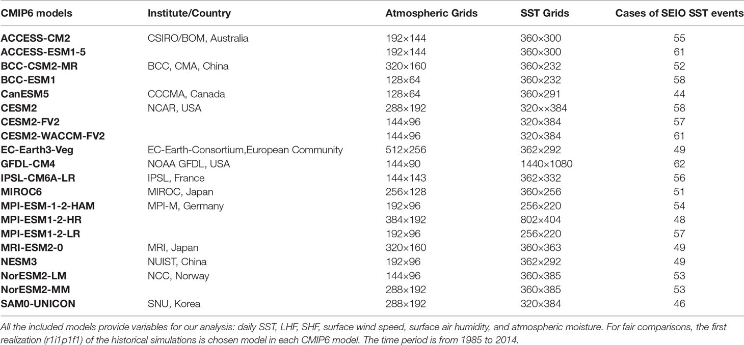
Table 1 List of CMIP6 models included in this study.

2.2 Method

Warm SST anomalies are favorable for energetic ocean–atmosphere interactions. However, warm SST anomalies alone do not guarantee such an impact, since the surface heat flux needs to be enhanced so that the atmosphere can feel the oceanic variation (Sobel et al., 2008). The LHF is estimated as (Cayan, 1992; DeMott et al., 2016)

L H F = ρ_{0} C_{d} L_{v} V (q_{s s t} - q_{a}) \dots (1),

where ρ₀ = 1.3kg/m³ is the air density; C_d = 1.35 × 10^-3 is the exchange coefficient for latent heat; L_v = 2.5 × 10⁶J/kg is the latent heat of vaporization; V is the wind speed near the surface; q_sst is the saturated specific humidity at the temperature of SST; and q_a is the near-surface specific humidity. q_sst is estimated with $\frac{ϵ}{p} A e^{- \frac{B}{T}}$ (Hendon and Glick, 1997), where p is the surface pressure, T represents SST, ε = 0.622, A = 2.53 × 10⁸ kPa, and B = 2.5 × 10⁶ K. Most variables can be decomposed into two scales. One is the low-frequency or the background component, which has a period longer than 100 days. The other one is the perturbation or the intraseasonal component with a period between 20 and 100 days. The high-frequency components with a period shorter than 20 days can also be included in the decomposition (Zhou and Murtugudde, 2014). However, none of the components containing the high-frequency variabilities are found to be large enough, so that they can be ignored. The background component is denoted with an overbar, and the intraseasonal component is denoted with a prime. For example, $T = \bar{T} + T^{'}$ . Therefore, the intraseasonal LHF can be written as

\begin{matrix} L H F^{'} = ρ_{0} C_{d} L_{v} [\bar{V} (\frac{ϵ}{p} A e^{- \frac{B}{\bar{T}}} \cdot \frac{B T^{'}}{{\bar{T}}^{2}} - q_{a}^{'}) (I) \\ + V^{'} (\frac{ϵ}{p} A e^{- \frac{B}{\bar{T}}} - {\bar{q}}_{a}) (II) & \dots (2) . \\ + V^{'} (\frac{ϵ}{p} A e^{- \frac{B}{\bar{T}}} \cdot \frac{B T^{'}}{{\bar{T}}^{2}} - q_{a}^{'})] (III) \\ + R_{L H F} (IV) \end{matrix}

Term I stands for the combined effects from SST anomalies and air humidity. Term II is for the impacts of intraseasonal surface wind anomalies. Term III denotes the impacts on LHF due to nonlinear interactions between intraseasonal SST and intraseasonal wind anomalies. R_LHF (Term IV) denotes the residual term.

To capture the development of equatorial convections, the moist static energy (MSE) and the MSE budget are also utilized. MSE is usually used as a proxy for atmosphere convections (Kiranmayi and Maloney, 2011). It is defined as m = C_p T_a + gz + L_vq where m is for MSE, C_p is the specific heat at constant pressure, T_a is the air temperature, g is the gravitational constant, z is the height above the surface, and q is the specific humidity. The intraseasonal MSE budget is written as (Maloney, 2009; Kiranmayi and Maloney, 2011)

\frac{\partial {〈 m 〉}^{'}}{\partial t} = H_{a d v}^{'} + V_{a d v}^{'} + L W^{'} + S W^{'} + L H F^{'} + S H F^{'} + R_{M S E} \dots (3),

where m denotes MSE; $〈 〉 = \int_{1000}^{100} dp$ denotes the vertical integral from 1,000 hPa to 100 hPa; $H_{a d v} = - 〈 {\vec{V}}_{H} \cdot \nabla m 〉$ is the horizontal advection, and ${\vec{V}}_{H}$ is the horizontal wind velocity; $V_{a d v} = - 〈 ω \frac{\partial m}{\partial p} 〉$ is the vertical advection, and ω is the vertical velocity; the vertically integrated longwave radiation (LW) and shortwave radiation (SW) are calculated as the differences of net fluxes between the top of the atmosphere and the sea surface; and R_MSE is the residual term.

The components of the involved variables are obtained by the Butterworth filter. The intraseasonal signals are applied with a 20–100-day band-pass filter, the background components are obtained by a 100-day low-pass filter. In order to show the key phenomena of the ocean–atmosphere interaction, the composite analysis is used, and all the intraseasonal signals are averaged with respect to the selected intraseasonal events. Pattern correlation is employed to diagnose the linear relation between two spatial patterns (Clodman, 1987; Lee and Kim, 2012; Zou and Zhou, 2016). The model fidelity of northward propagation is quantified by the pattern correlation coefficient (PCC) between CMIP6 simulation and observation (Li et al., 2021). The statistical significances of both PCC and the composite analysis are tested with the Student’s t-test. The effective number of degrees of freedom is determined following the modified Chelton method (Pyper and Peterman, 1998).

3 Results

3.1 Biases of CMIP6 Model Simulations

The biases for precipitation are still obvious in the 6th Coupled Model Inter-comparison Project (CMIP6; Eyring et al., 2016). The simulated intraseasonal variance of monsoon precipitation is smaller than the observation in most models. The standard deviation (STD) of intraseasonal rainfall anomalies in 14 out of total 20 CMIP6 models is lower than 12 mm/day (Figures 1C, F–L, P–U), while the observed rainfall STD reach up to 21 mm/day (Figure 1A). Thus, for 70% of the CMIP6 models, the intraseasonal rainfall anomalies are around half of the observation.

FIGURE 1

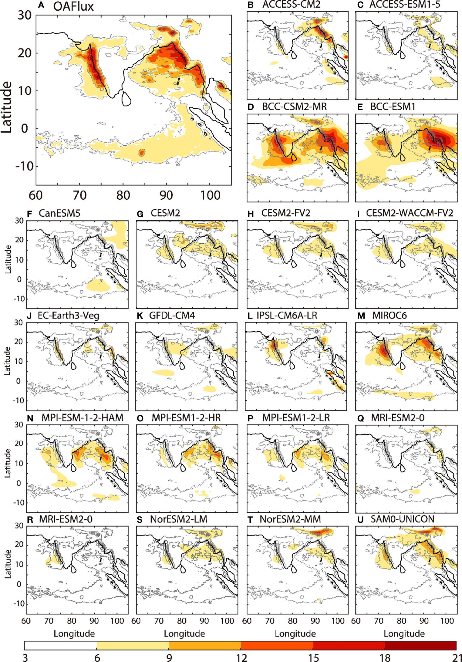
Figure 1 Intraseasonal standard deviation (STD) of precipitation (unit: mm/day) during JJAS: (A) TRMM, (B–U) CMIP6 outputs. The gray contours are TRMM STD from 6 to 18 mm/day with an interval of 3 mm/day.

Correspondingly, the model biases are also clear in the ocean–atmosphere interaction, for example, over the SEIO. Statistically, the oceanic impacts on the atmosphere can be simply quantified with the correlation between the SST anomalies and the sum of latent heat flux (LHF) and sensible heat flux (SHF; Cayan, 1992; Xi et al., 2015). For example, according to Xi et al. (2015) and Vialard et al. (2008), when there is a positive correlation between SST anomalies and the sum of LHF and SHF anomalies, the ocean drives the atmosphere. In the CMIP6 models in which the daily variables (SST, LHF, SHF, and precipitation) are available, such correlations during ISM (from June to September) at intraseasonal timescales are shown in Figure 2. Compared with observations (Figure 2A), pronounced differences occur over the southeastern Indian Ocean (SEIO) within 75°E–95°E and 15°S–5°S. In nature, the significant correlation coefficients larger than 0.6 indicate that the ocean plays an active role during ISM. In contrast, the correlation coefficients between intraseasonal SST anomalies and the intraseasonal SHF + LHF in CMIP6 models are generally smaller than 0.2 and are not statistically significant (Figures 2B–U).The bias of model simulations calls for further exploration on the ocean–atmosphere interaction over the southeastern Indian Ocean (SEIO) and the associated connection with the monsoon rainfall.

FIGURE 2

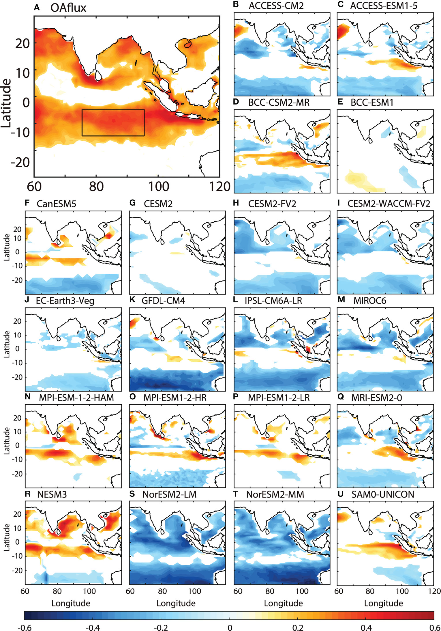
Figure 2 Ocean–atmosphere interactions at intraseasonal time scales during JJAS. Colors are the intraseasonal correlations between SST and LHF+SHF in (A) OAFlux and (B–U) CMIP6 outputs. All signals are statistically significant at a 95% confidence level. The black box in Figure 1A denotes the region with pronounced air–se interaction in the southeastern Indian Ocean (SEIO, 75°E–95°E, 15°S–5°S).

3.2 Local Intraseasonal SST Impacts Over SEIO

The standard deviations (STDs) of intraseasonal SST anomalies are shown in Figure 3. They are pronounced over the SEIO during boreal summer (June–September, JJAS; Li et al., 2008; Vinayachandran and Saji, 2008; Liang et al., 2018). The region (75°E–95°E and 15°S–5°S, black box in Figures 2A, 3) with an active oceanic impact and a large variance of intraseasonal SST anomalies is selected. The regional mean intraseasonal SST anomalies over 75°E–95°E and 15°S–5°S are shown in Figure 4. They are used as a reference for the following composite analysis. The days, when the regional mean SST anomalies over the black box (Figure 2A) reach the local maximum and are larger than the STD of the reference, are regarded as the day 0 of the warm SST events. There are a total of 62 events from 1985 to 2014 (red circles in Figure 4).

FIGURE 3

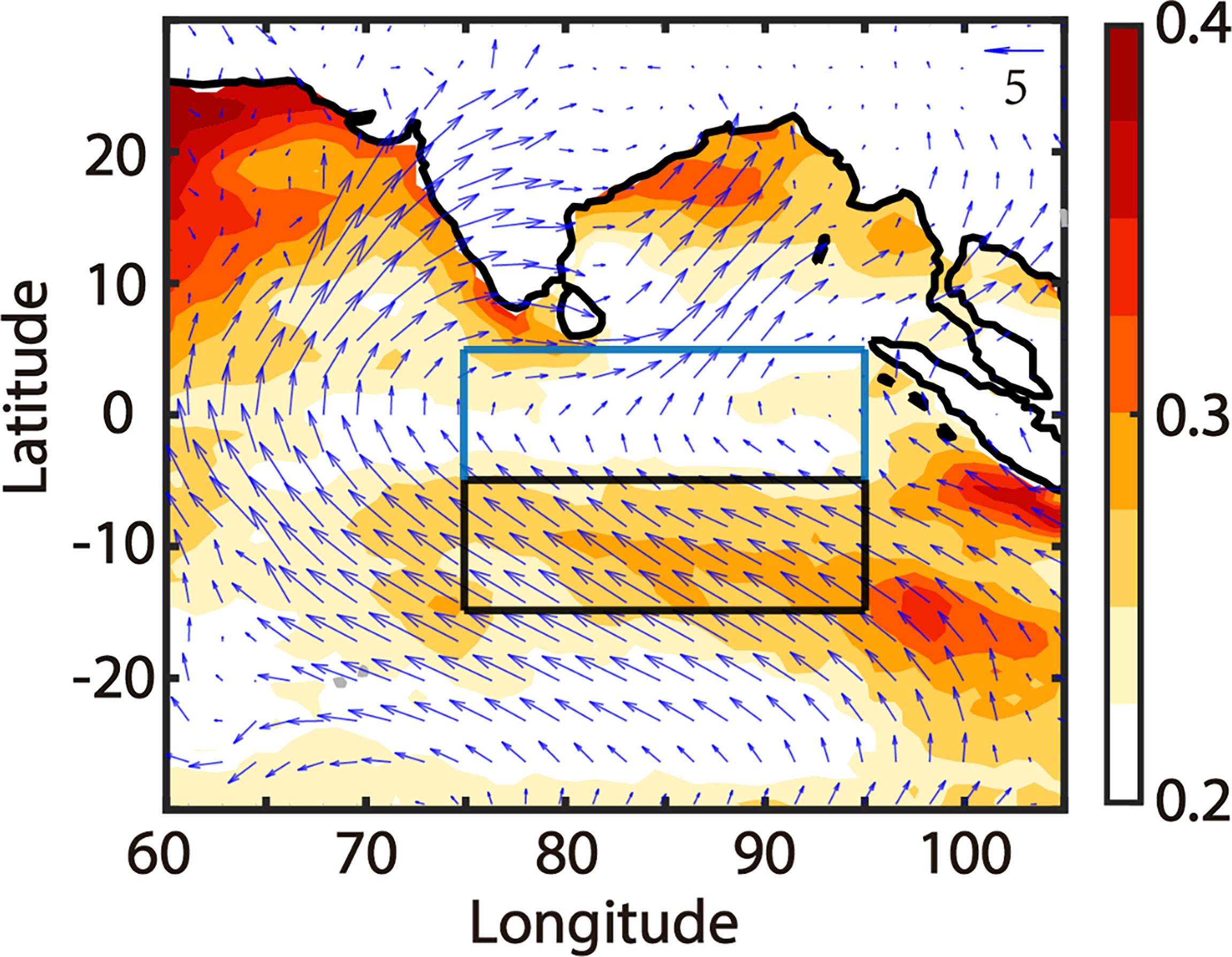
Figure 3 The STD of intraseasonal SST anomalies (colors, unit: °C) and climatological surface wind vectors during boreal summer (arrows, unit: m/s). The black box is the same as the black box in Figure 1A (75°E–95°E, 15°S–5°S), over which one can also see the pronounced variation of intraseasonal SST anomalies. The blue one is the region in the equatorial Indian Ocean (EIO, 75°E–95°E, 5°S–5°N).

FIGURE 4

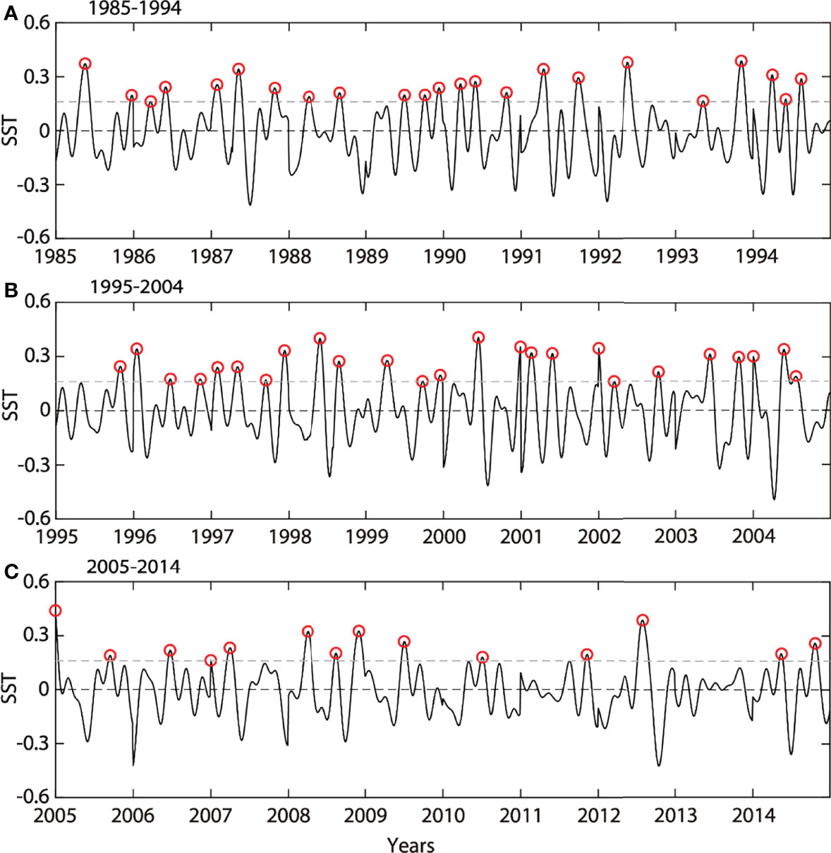
Figure 4 Intraseasonal SST (black curves, unit: °C) anomalies averaged within 75°E–95°E and 15°S–5°S during ISM (June–September) from OAFlux within 1985-1994 (A), 1995-2004 (B) and 1995-2014 (C).

The composite intraseasonal SST, LHF, and surface wind anomalies averaged on day 0 are shown in Figure 5A. On day 0, warm SST anomalies reach 0.3°C over SEIO, and the LHF is reinforced due to warm SST anomalies, as shown with the black contours in Figure 5A. The composite regional mean LHF over SEIO (15°S–5°S and 75–95°E, black box in Figure 3) and the decomposition following Eq. (2) are shown in Figure 6A. Starting from day −8, warm SST anomalies occur over SEIO (yellow curve in Figure 6C), and LHF increases accordingly (Term I and yellow line in Figure 6A). Around day 0, the enhancement of LHF due to Term I reaches the maximum since the SST anomalies reach the maximum (yellow curve in Figure 6C). Generally, Term I consists of two parts [refer to Eq. (3)], the SST effects on LHF $(T e r m_{S S T} = ρ_{0} C_{d} L_{v} \bar{V} \cdot \frac{ϵ}{p} A e^{- \frac{B}{\bar{T}}} \cdot \frac{B T^{'}}{{\bar{T}}^{2}})$ and the near-surface air humidity on LHF $(T e r m_{a} = ρ_{0} C_{d} L_{v} \bar{V} q_{a}^{'})$ . The variation of both two terms are shown in Figure 6C. However, it is clear that SST effects play a dominant role (dark blue curve in Figure 6C) over SEIO, and Term_SST can reach up to 10 W/m², while the associated Term_a is confined within ±2 W/m². After day 0, the warm SST anomalies reduce, and the oceanic contribution to the LHF also diminishes.

FIGURE 5

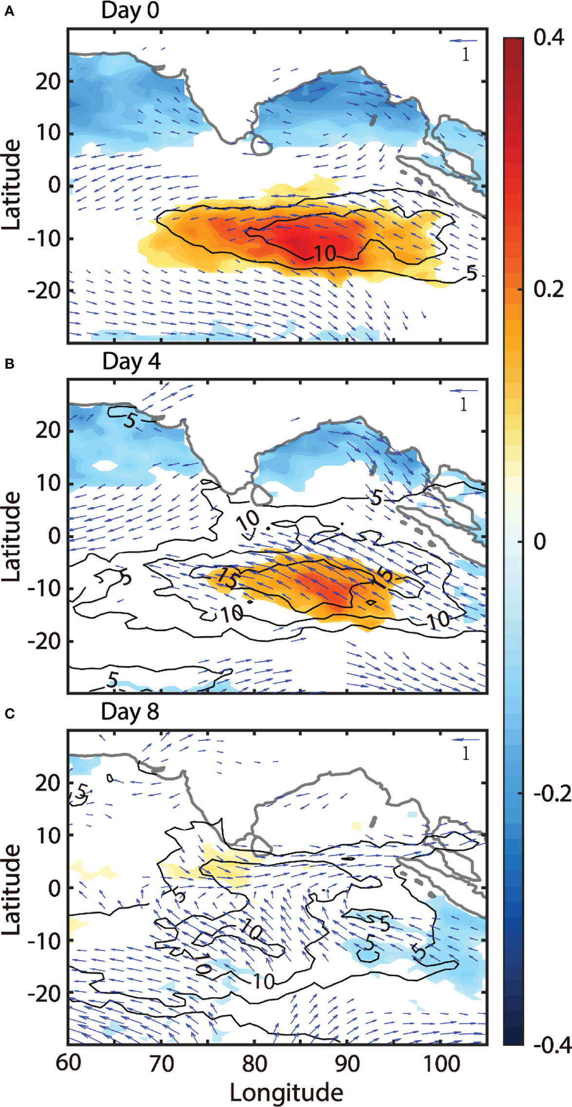
Figure 5 The composite of intraseasonal SST (colors, unit: °C), LHF (black contours, unit: W/m2) and surface wind (blue arrows, unit: m/s) anomalies on Days 0 (A), 4 (B), and 8 (C).

FIGURE 6

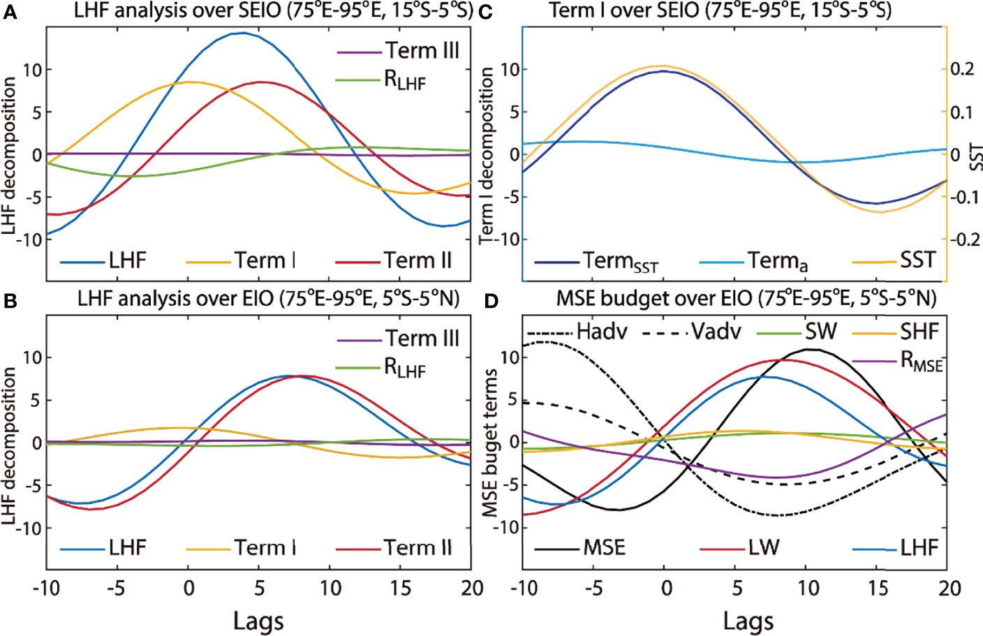
Figure 6 (A) Decomposition of intraseasonal LHF (unit: W/m²) averaged over SEIO. LHF is denoted with the blue curve. Term I (yellow curve) and Term II (red curve) denote the latent heat anomalies induced by SST anomalies and wind anomalies, respectively. Term III (purple curve) denotes the perturbations coming from both wind and SST anomalies. R_LHF (green curve) is the residual term. (B) is the same as (A), but over Equatorial Indian Ocean (EIO, the blue box in Figure 3). (C) is the same as (A), but for the decomposition of Term I (blue curves, unit: W/m²) and intraseasonal SST anomalies (yellow curve, unit: °C) over SEIO. In Eq. (3), Term I can be decomposed as the difference of $T e r m_{S S T} = ρ_{0} C_{d} L_{v} \bar{V} \cdot \frac{ϵ}{p} A e^{- \frac{B}{\bar{T}}} \cdot \frac{B T^{'}}{{\bar{T}}^{2}}$ (dark blue curve) and $T e r m_{a} = ρ_{0} C_{d} L_{v} \bar{V} q_{a}^{'}$ (light blue curve). (D) Integrated MSE budget averaged within EIO. Black curve represents MSE (unit: 10⁶ J/m²). Black dot-dashed curve represents the horizontal MSE advection; black dashed one represents the vertical MSE advection (unit: W/m²). Red, green, blue, and yellow curves are longwave radiation, shortwave radiation, LHF, and SHF (unit: W/m²), respectively. Purple curve is the residual term.

However, the increase in LHF does not terminate. Instead, it is boosted by the increase in surface winds. Around day 0, southeasterly wind anomalies begin to grow over the warm SST anomalies (arrows in Figure 5A). The southeasterly wind anomalies enhance the total winds, since the background winds are also southeasterly over SEIO (arrows in Figure 3A). The influences of warm SST anomalies on accelerating the low-level winds are common during ocean–atmosphere interactions. According to Chelton et al. (2001); Xie (2004), and Small et al. (2008), the SST modifications are responsible for increasing instability and enhancing vertical mixing in the atmospheric boundary layer, which transport momentum from the upper boundary layer to the sea surface, and finally, the surface wind speed increases (Hayes et al., 1989; Maloney and Chelton, 2006; Chelton et al., 2007 and so on). The increment of surface wind speed gives rise to the positive anomalies of latent heat flux around day 0 over SEIO (Term II, red line in Figure 6A), which agrees with the positive wind-evaporation-SST (WES) feedback (Neelin et al., 1987; Xie and Philander, 1994). Consistently, the total latent flux keeps growing on day 4 over SEIO (blue line in Figure 6A), although the area with warm SST anomalies shrinks (yellow line in Figure 6B). In the decomposition of LHF, the influences from other terms are not strong. For instance, in Figure 6A, the interaction between the intraseasonal SST and intraseasonal winds is small [Term III in Eq. (2) and purple line in Figure 6A]. The residual term in Eq. (2) is also small [R_LHF in Eq. (2) and green line in Figure 6A).The warm intraseasonal SST anomalies are constrained over the SEIO. However, the consequent southeasterly wind anomalies extend from the SEIO to the deep tropics. As shown in Figure 5B, southeasterly wind anomalies prevail over SEIO. On day 4, the LHF propagates equatorward along with the surface winds, although the warm SST anomalies reduce over SEIO and have no evidence of propagating northward. The equatorward propagations of surface wind anomalies and LHF reach the equator around day 4, as the southerly component of surface wind anomalies and LHF at the values of 10 W/m² begin to occur over the equator on day 4 (contours and vectors in Figure 5B). The signals of wind anomalies and LHF persist until day 8, as the southerly component of wind anomalies and larger LHF prevail within 0° to 5°N on day 8 (contours and vectors in Figure 5C). The decomposition of LHF in Eq. (2) over the equatorial Indian Ocean (EIO, within 75°E–95°E and 5°S–5°N; blue box in Figure 3) is shown in Figure 6B. The total LHF anomalies over EIO appear 3 days after that over SEIO and reach the local maximum around day 7 (blue line in Figure 6B). A key difference in the decomposition of the LHF between SEIO (Figure 6A) and EIO (Figure 6B) resides in the influence of SST anomalies. Warm SST anomalies over EIO are not significant (Figure 5B). Thus, their impact on the LHF is small [Term I in Eq. (2) and yellow line in Figure 6B]. In contrast, the southeasterly winds extend to the equatorial region, which plays a dominant role in the variation of LHF [Term II in Eq. (2) and red line in Figure 6B]. This is consistent with previous studies by Araligidad and Maloney (2008); Grodsky et al. (2009), and Gao et al. (2018) that, within the equatorial region, the variation in intraseasonal LHF is mainly attributable to atmospheric wind anomalies rather than to the oceanic thermal effects.

3.3 The Enhanced Equatorial Atmospheric Convection

Over EIO (75°E–95°E, 5°S–5°N), the atmosphere becomes unstable due to the enhanced LHF. The moist static energy (MSE) is usually a good proxy for the development of atmospheric convection (Kiranmayi and Maloney, 2011). The budget of intraseasonal MSE is helpful for detecting the influential factors [see Eq. (3); Maloney, 2009; Kiranmayi and Maloney, 2011]. Figure 6D shows the regional mean of each term in Eq. (3) over 75°E–95°E and 5°S–5°N. The column-integrated MSE (black solid curve) over the deep tropics reaches the maximum around day 10, which denotes the mature phase of the equatorial convection. During the growth of MSE from day 0 to day 10, the effects from longwave radiation (LW, red curve in Figure 6D) and LHF (blue curve in Figure 6D) are obvious, and they play dominant roles. LW plays a primary role and denotes the contribution of longwave heating during the atmospheric cumulus convective development (Kiranmayi & Maloney, 2011). LHF also plays an important role, which is associated with the contribution of intraseasonal wind anomalies from the sea surface. The other components, such as the horizontal (black dot dashed curve in Figure 6D) and vertical (black dashed curve in Figure 6D) advection are moderate from day 0 to day 10. The shortwave radiation (SW, green curve in Figure 6D) and SHF (yellow curve in Figure 6D) are tiny. The dominant roles of LW and LHF over tropical Indian Ocean are also consistent with other MSE budget analyses during the period of MJO during boreal winter (DeMott et al., 2016) and MISO/BSISO in the boreal summer (Gao et al., 2018). Moreover, in this study, the enhancement of LHF is attributable to the warm SST anomalies over SEIO. The intraseasonal oceanic effects on the atmosphere are not confined locally in SEIO. Instead, they are transported by the wind anomalies and support the atmospheric convection in the deep tropics.

3.4 Cross-Equatorial Influence on the ISM Rainfall

The equatorial convection triggered by the enhanced LHF propagates northward as MISO during boreal summer, which is an important trigger of intraseasonal variabilities over the Indian subcontinent (Karmakar and Krishnamurti, 2018; Qin et al., 2020; Qin et al., 2021; Li et al., 2022a). In Figure 7A, the Hovmöller diagrams of observed LHF (contours) and satellite-based rainfall (colors) anomalies during active convection are shown with respect to day 0. To match up with the time domain of TRMM dataset, the day 0s are obtained within 1998–2014 (red circles in Figure 4). Noteworthy, these involved day 0s (or cases) are not those events selected by the pronounced intraseasonal variabilities in the monsoon region (e.g., the intraseasonal rainfall anomalies over Bay of Bengal, Li et al., 2022b; Zhou et al., 2017a), which were commonly used in many previous studies (Suhas et al., 2012; Girishkumar et al., 2017). One can see that the northward propagations of LHF and precipitation from the equator to the monsoon region are closely related to the intraseasonal warm SST anomalies over SEIO (Figure 7A). As mentioned before, positive LHF anomalies (contours) occur around the peak of warm SST anomalies over SEIO (day 0) and then spread northwestward to the equator. The equatorward intraseasonal wind anomalies along with LHF reach the equator and support the development of equatorial convection (colors) around day 10. Under the support of easterly vertical wind shear (Jiang et al., 2004) and atmospheric meridional advection (Bellon and Sobel, 2008), the enhanced tropical convection spreads northward as MISO and positive rainfall anomalies are induced over the monsoon region.

FIGURE 7

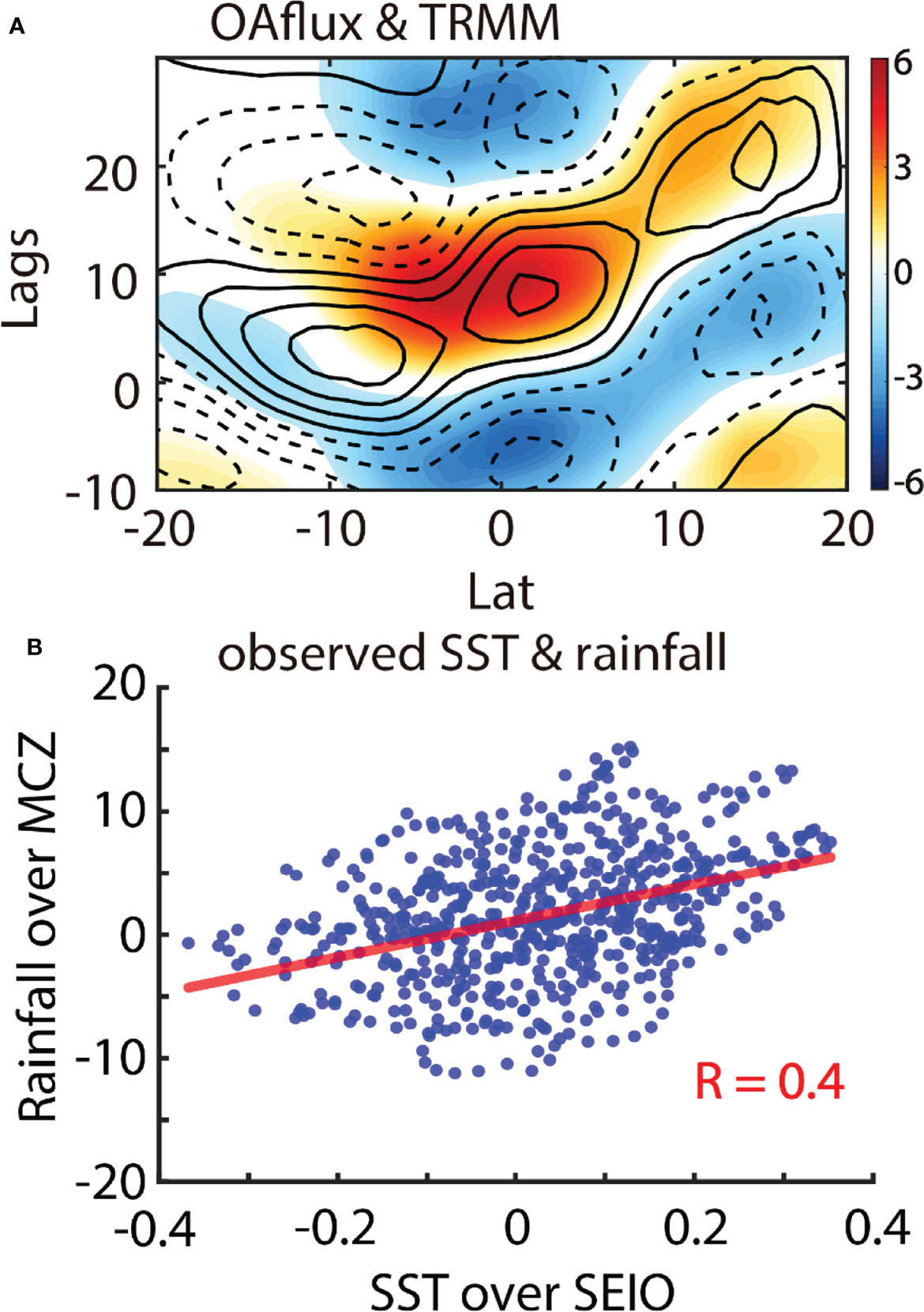
Figure 7 (A) Composite Hovmöller diagrams of intraseasonal rainfall (colors, unit: mm/day) and LHF (contours, unit: W/m²) anomalies averaged within 75°E–95°E. LHF from OAFlux and rainfall from TRMM. The dashed contours for LHF are from −12 to −4 W/m², and the solid contours are from 4 to 16 W/m². The interval is 4 W/m². (B) The relationship between the intraseasonal SST anomalies over SEIO and the intraseasonal rainfall over MCZ (75°E–95°E, 10°N–20°N). The blue dots are obtained from the observed cases during 1998–2014 (red circles in Figure 4). For each case, the intraseasonal SST anomalies from Day −10 to Day 10 are shown along the x-axis. The y-value of each blue dots is the corresponding intraseasonal rainfall in MCZ after 20 days (Days 10–30). The red line is estimated by the least square fit, and the correlation coefficient is statistically significant at a confidence level of 95%.

Statistically, the variation of the intraseasonal rainfall anomalies over the monsoon core zone (MCZ, 75°E–95°E, 10°N–20°N) in the Northern Hemisphere also has a positive correlation with that of the warm SST anomalies over SEIO in the Southern Hemisphere. In Figure 7B, the blue dots are obtained from the intraseasonal events during 1998–2014, which are the same as those in the composite of Figure 7A. For each case, the variation of the intraseasonal SST anomalies from day −10 to day 10 are shown as the x-values of the blue dots. The y-values are the corresponding intraseasonal rainfall in MCZ after 20 days (days 10–30). In total, there are 31 cases and 651 blue dots in Figure 7B. The red line is estimated by the least square fit, and the correlation coefficient is 0.4, which is statistically significant at a confidence level of 95%.

The correlation coefficient of 0.4 indicates that the above cross-equatorial process is not a predominant contributor but is inevitable to the monsoon rainfall events. The above correlation coefficient is not as high as the ones obtained from the traditional monsoon modes (Lee et al., 2012; Suhas et al., 2012; Zhou et al., 2017a). For example, a recent Central Indian Ocean (CIO) mode is apt at capturing the northward propagation and has a high correlation with the monsoon rainfall over the Bay of Bengal (Zhou et al., 2017a; Zhou et al., 2017b; Qin et al., 2021). The value of 0.4 for the cross-hemisphere implies that the relation between SEIO and MCZ is not the one-to-one correspondence as the above tradition ones. In other words, the cross-hemispheric impact from SEIO on MCZ is not the most dominant mechanism for the monsoon rainfall events. Instead, it is a good complement to the recent widely accepted mechanisms for MISO like vertical shear of easterly wind (Jiang et al., 2004) and atmospheric meridional advection (Bellon and Sobel, 2008) and can help to ameliorate the urgent need of the recent climate models that shows a clear bias of monsoon rainfall (Figure 1).

3.5 The Bias of CMIP6 and Probable Reason

The performance of CMIP6 can be checked in Figure 8, which is a similar Hovmöller diagram as in Figure 7A. The warm SST events over SEIO are obtained separately in each CMIP6 output following the routes described in Figure 4. The case numbers of each CMIP6 model within 1985–2014 are shown in Table 1. The numbers of the simulated cases are close to the observed one.

FIGURE 8

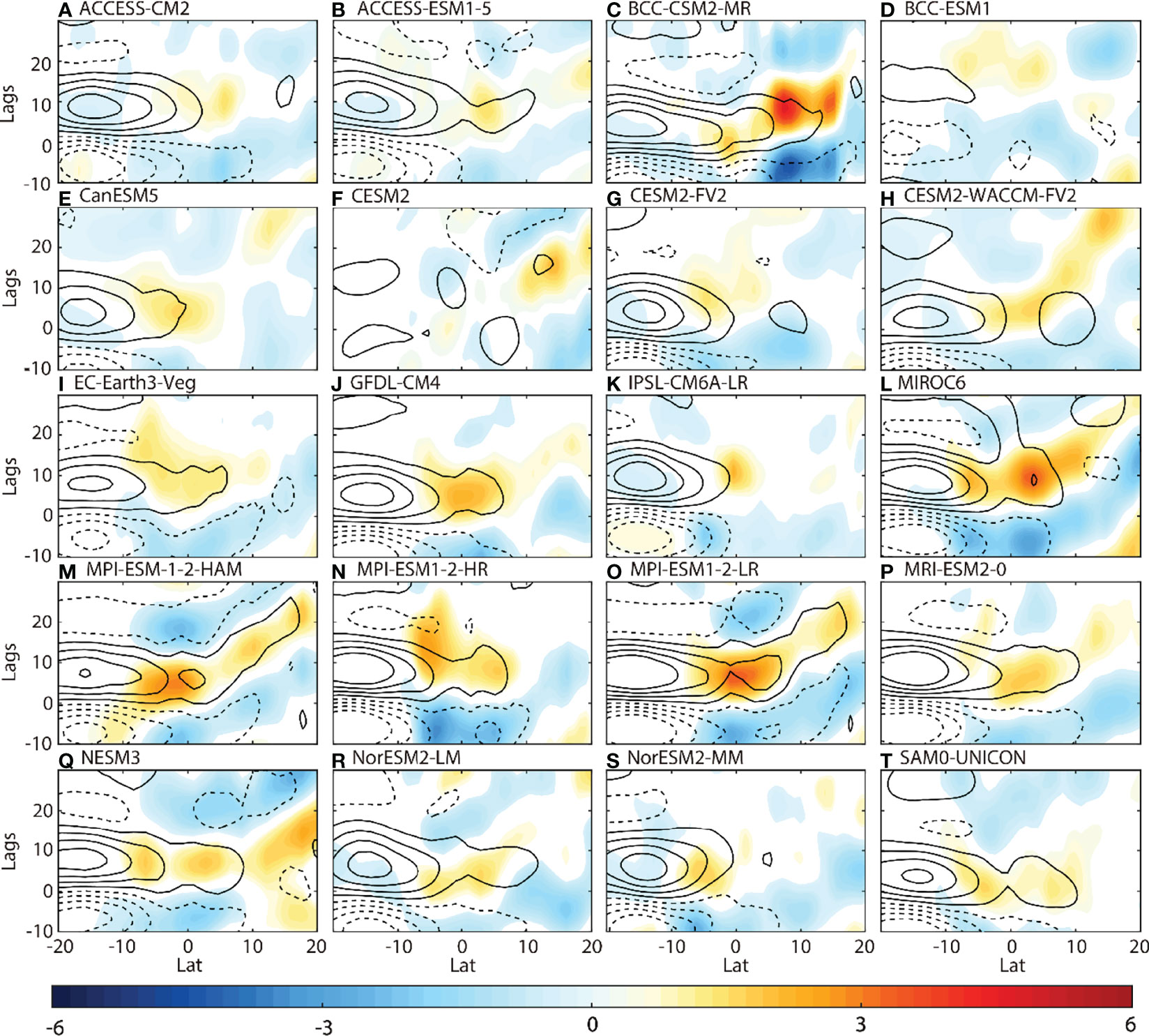
Figure 8 The same figures as Figure 7A, but for CMIP6 outputs. The contours for LHF are from −28 to −4 W/m² (dashed contours) and from 4 to 28 W/m² (solid contours) with an interval of 8 W/m². All signals shown are statistically significant at a 95% confidence level.

Obviously, in CMIP6, the northward propagations from the equator to the monsoon region are not well simulated, especially the intensity (colors in Figure 8). Compared to the observation, the intensities of northward propagations in nearly all the CMIP6 are much weaker or even insignificant. The observed northward propagation starts from the equator around day 10 (reddish in Figure 7A). At the initial stage of MISO, the observed equatorial rainfall anomalies are ~5 mm/day. In contrast, all the CMIP6 simulations are only 1–3 mm/day (reddish in Figure 8), which is only half of the observations. That the simulated tropical rainfall in CMIP6 is weaker than the observations is partially attributable to the bias in the above air–sea interactions over SEIO. In reality, strong equatorial convections are nourished by the equatorward LHF anomalies originating from SEIO. However, in CMIP6 (Figure 8), LHF anomalies are trapped over the southern Indian Ocean (20°S–0°) from day 0 to day 15, and they do not propagate equatorward (contours in Figure 8). As a result, the deep tropics lack energy for convection in simulations, which also explains why the CMIP6 models yield small STD of intraseasonal rainfall anomalies around the equator (Figures 1B–U).Despite the systematic deficient simulations over SEIO in CMIP6, results still show the importance of ocean–atmosphere interaction over SEIO on the equatorial rainfall anomalies and the northward propagation. The relationship between simulated SST anomalies over SEIO and simulated rainfall anomalies over EIO is shown in Figure 9A. Each blue dot in Figure 9A represents one of the CMIP6 model outputs. The x-value of a blue dot is the warm SST anomaly averaged over SEIO and on day 0 of all the selected events in each CMIP6 model (Table 1). The y-value is the rainfall anomaly averaged over EIO and on day 10, correspondingly. The linear regression is shown with a red line, and the correlation coefficient is 0.72, which is statistically significant at a confidence level of 95%. It denotes that stronger ocean–atmosphere interactions over SEIO are favorable for larger equatorial rainfall anomalies in CMIP6 models. On the other hand, when the equatorial rainfall anomalies are well simulated, the simulated northward propagation will become more realistic. The relationship between SST anomalies over SEIO and northward propagation is shown in Figure 9B. Here, the northward propagation is quantified as the pattern correlation coefficient (PCC) between the northward propagation of each CMIP6 model and the observation (Clodman, 1987). Specifically, the calculation of PCC is based on the northward propagation of rainfall anomalies within 0°–20°N in each panel of Figure 8 and the associated observation in Figure 7A. It is clear that there is a positive correlation between SST anomalies over SEIO and PCC, and the significant correlation coefficient is 0.67.

FIGURE 9

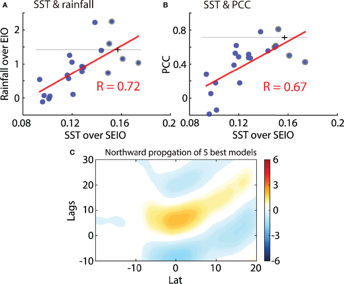
Figure 9 The scatter plots for intraseasonal SST anomalies averaged on Day 0 over SEIO against (A) the intraseasonal rainfall anomalies averaged on Day 10 over EIO and (B) the pattern correlation coefficient (PCC) of northward propagation for each CMIP6 model. PCC is calculated by the simulated northward propagation of rainfall anomalies within 0°–20°N in each panel of Figure 8 and the associated observation in Figure 7A. The red lines are estimated by the least square fit. The correlation coefficients are (A) 0.72 and (B) 0.67, which are statistically significant at 95% confidence level. The blue dots marked with gray edges in (A, B) are the five CMIP6 models (MIROC6, MPI-ESM-1-2-HAM, MPI-ESM1-2-LR, GFDL-CM4, and MRI-ESM2-0) with the warmest SST anomalies over SEIO. The black plus in (A) denotes the rainfall anomalies of the five CMIP6 models on Day 10 over EIO, and the gray line in (A) denotes the value of 1.47 mm/day. The black plus in (B) denotes the PCC with respect to the averaged northward propagation of the five CMIP6 models (C) and Figure 7A. The gray line in (B) denotes the PCC value of 0.73. (C) The same figure of northward propagation as Figure 8, but for the above five CMIP6 models. The signals in (C) are statistically significant at a 95% confidence level.

In this way, if the model simulations can provide a better simulation of SST anomalies over SEIO, the associated ocean–atmosphere interaction will prompt stronger equatorial convection and larger precipitation in 10 days, which will lead to more realistic northward propagation of ISVs and heavier summer rainfall over monsoon region. For example, the top 5 models with the warmest SST anomalies over SEIO can reproduce more realistic northward propagating MISOs, which exceeds at least 85% of the CMIP6 models. The five CMIP6 models are MIROC6, MPI-ESM-1-2-HAM, MPI-ESM1-2-LR, GFDL-CM4, and MRI-ESM2-0 (the circles with gray edges in Figures 9A, B). The composite Hovmöller diagram of intraseasonal rainfall anomalies is shown in Figure 9C. Over EIO, the mean rainfall anomaly on day 10 is 1.47 mm/day (also see black plus in Figure 9A). It is also denoted as the gray line in Figure 9A. There are only 3 of 20 CMIP6 outputs exceeding the gray line. In other words, the averaged equatorial rainfall of the top 5 models is stronger than 85% of the total 20 CMIP6 results. With stronger equatorial convections, the northward propagation is closer to nature, too (Figure 9C). The PCC between Figure 9C and the observed northward propagation in Figure 7A is 0.73 (black plus and gray line in Figure 9B). In total, 18 of 20 blue dots are under the gray line. That is, the northward propagation of the best five models is more realistic than 90% of the total 20 CMIP6 models. Therefore, as for CMIP6 models, further attention on the ocean–atmosphere interaction over SEIO is of great importance for better simulations of monsoon rainfall.

4 Conclusions and Discussion

In contemporary climate models, the weak Indian summer monsoon rainfall is a common bias. Consistently, the simulated northward-propagating MISO and the tropical convection are also weaker in boreal summer (Ahn et al., 2017, also see Figure 1). It is shown in this study that the cross-equatorial influences originating from the warm SST anomalies over the SEIO are prone to strengthen the tropical convection and consequently the precipitation in the Indian monsoon region. Warm intraseasonal SST anomalies over SEIO support local enhancement of the intraseasonal southeasterly wind anomalies and the latent heat flux. The southeasterly wind anomalies propagate equatorward from the Southern Hemisphere, although the warm SST anomalies are constrained to SEIO. The total winds get reinforced, since the intraseasonal wind anomalies share the same direction as the background winds. Due to the WES feedback, the LHF increases from SEIO to the deep tropics, along with the equatorward propagation of wind anomalies. As a result, the MSE increases around the equator, and the tropical convection becomes stronger. During boreal summer, the enhanced tropical convections propagate northward and cause extreme rainfall events over monsoon regions. Current results indicate that the inter-hemispheric impacts are an inevitable contributor to the heavy rainfall during ISM in the subtropics in the Northern Hemisphere. However, such process understanding is not well captured in CMIP6 models, which is one reason for the less simulated ISM rainfall than observations.

The unsatisfactory simulations of CMIP6 are associated with the defective ocean–atmosphere interaction over SEIO (Figure 2). One clue is that the variances of intraseasonal SST anomalies are feeble and far from the observations (Figure 10). The STD of simulated intraseasonal SST anomalies in most CMIP6 models is hardly larger than 0.15°C, which is about half of the observations. The weak SST anomalies are not powerful enough to drive the response in the low-level troposphere. As a result, the oceanic impact on the atmosphere cannot be captured in most CMIP6 models. However, most CMIP6 models do not provide oceanic variables, such as the 3-D temperature and currents. Thus, it is hard to apply a full heat budget analysis in the upper mixed layer and to detect the reasons dynamically. Moreover, there are many other reasons for the intraseasonal biases over SEIO, such as the geography of the southeastern Indian Ocean and the confluence of the Indian Ocean Dipole Mode (Saji et al., 1999; Murtugudde et al., 2000), South Equatorial Current and Indonesian Throughflow (Gordon et al., 1997; Murtugudde et al., 1998), the South Java Current (Quadfasel and Cresswell, 1992), and the feedbacks with Indonesian rainfall (Hendon, 2003). The complicated ocean environment increases the difficulty of a satisfactory simulation. The biases in climatological wind and SST over SEIO are other important concerns (Lee et al., 2013; Li et al., 2015), which are also possible reasons for weaker high-frequency signals like intraseasonal oscillations.

FIGURE 10

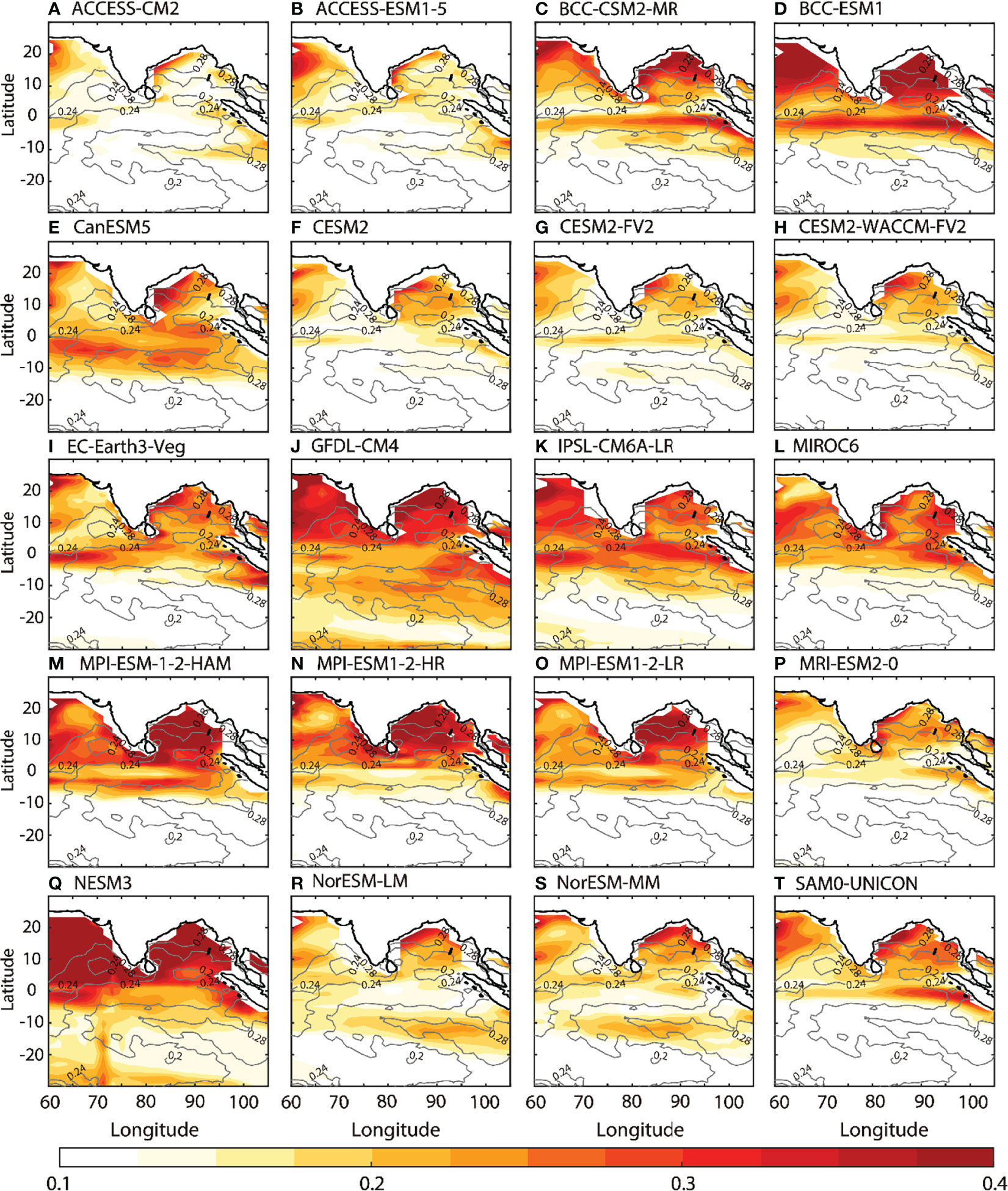
Figure 10 Intraseasonal STD of SST (unit: °C, colors) anomalies within Indian Ocean during boreal summer for CMIP6 outputs. The gray contours are the observed STD of intraseasonal SST anomalies from OAFlux.

Data Availability Statement

The original contributions presented in the study are included in the article/supplementary material. Further inquiries can be directed to the corresponding author.

Author Contributions

ZM, LZ, JQ, and BL contributed to the conception and design of the study. All authors contributed to the article and approved the submitted version.

FUNDING

This work is supported by grants from National Natural Science Foundation of China (42076001 and 42106003).

Conflict of Interest

The authors declare that the research was conducted in the absence of any commercial or financial relationships that could be construed as a potential conflict of interest.

Publisher’s Note

All claims expressed in this article are solely those of the authors and do not necessarily represent those of their affiliated organizations, or those of the publisher, the editors and the reviewers. Any product that may be evaluated in this article, or claim that may be made by its manufacturer, is not guaranteed or endorsed by the publisher.

Acknowledgments

Constructive and valuable comments from the reviewers are greatly appreciated.

References

Ahn M.-S., Kim D., Sperber K. R., Kang I.-S., Maloney E. D., Waliser D. E., et al. (2017). MJO Simulation in CMIP5 Climate Models: MJO Skill Metrics and Process-Oriented Diagnosis. Clim. Dyn. 49, 4023–4045. doi: 10.1007/s00382-017-3558-4