Vertical structural variability of diurnal internal tides inside a mesoscale anticyclonic eddy based on single virtual-moored Slocum glider observations

The vertical structural variability of the diurnal internal tide (DIT) with a mode-1 wavelength of ~420 km inside a mesoscale baroclinic anticyclonic eddy was examined based on observations by a single virtual-moored (VM) Slocum glider. During the glider observational period from 10 to 19 September 2018, the eddy traveled northward at approximately 50 km, allowing the glider to scan a cross section of 50 km wide and 800 m deep inside the eddy. VM observations showed that DIT experienced a noticeable vertical structural variability near the eddy center. In a range of 30 km horizontally from the eddy center (inner center), DIT’s vertical displacements were significantly intensified in the 400–800-m depth below the eddy. In the range of 30–50 km from the eddy center (outer center), DIT was almost uniformly distributed from the surface to 800-m depth. Owing to the spatiotemporally restricted dataset by the glider, the significance of DIT’s modulation observed inside the eddy can be questionable. As a result of comparing DIT’s vertical structural variability in two domains in terms of available potential energy (APE) and horizontal kinetic energy (HKE) using CTDs inside the eddy and ADCPs outside the eddy, DIT’s vertical structure inside the eddy was significantly distinguished from that outside the eddy. The relative vorticity inside the eddy was estimated based on the satellite dataset; it was negatively great in the inner center (approximately 0.35 – 0.25f) and small in the outer center (approximately 0.2 – 0.1f). These observational behaviors indicate a close relationship between them; the vorticity-dependent modulation of the DIT seems to be observationally confirmed inside the eddy. Further, in order to examine the energy transferring behavior in low vertical modes, a wavenumber spectral analysis was performed on the DIT displacements and the lowest four wavenumbers, K_z (1) through K_z (4), showed a similar behavior to those observed in DIT’s vertical structural variability inside of the eddy; the relative power of the sum of K_z (2) ~ K_z (4) with respect to K_z (1) was strong in the inner center and weakened in the outer center. These results seem to support that the wave–eddy interaction is non-uniform inside the eddy and partially depends on the relative vorticity.

Introduction

Internal waves oscillating in a stratified fluid interior are prevalent in the ocean and play various roles in modulating the ocean environment. Internal waves with tidal frequency are called internal tides (ITs), mostly generated via barotropic tide–bathymetry interactions, that contribute to diapycnal mixing in the deep ocean (Munk and Wunsch, 1998; Egbert and Ray, 2000; Wunsch and Ferrari, 2004) and nutrient supply (Villamana et al., 2017) and are believed to transport considerable amounts of energy over hundreds to thousands of kilometers from the generation site (Alford, 2003; Tian et al., 2003). This long-range propagation creates multiple encounters with mesoscale eddies and currents, through which their propagation speeds and directions are modified (Alford et al., 2012; Nash et al., 2012; Kerry et al., 2014). Owing to these modulations and remote generation, a considerable fraction of internal tides is unpredictable in many locations (Alford et al., 2012; Nash et al., 2012; Kelly and Lermusiaux, 2016).

A multitude of studies have been conducted on the interactions between internal waves and mesoscale eddies, which are known to play critical roles in modulating ITs. According to Bühler and Mclntyre (2005), internal waves can lead to deformation and eventual breaking via a wave-capture mechanism, wherein internal wave packets permanently extract energy from a geostrophic eddy field. Chavanne et al. (2010) used the ray tracing method to investigate the propagation of internal waves passing through a mesoscale current: a cyclone of 55-km diameter and ~100-m vertical decay scale. Their investigations showed that an idealized mesoscale cyclone intensified internal wave energy at the surface by a factor of 15 and decreased the vertical wavelength by a factor of 6, showing a qualitative consistency with observations of semidiurnal surface currents in the Kauai Channel. Whalen et al. (2012) examined Argo profiles and suggested that internal waves interacting with the eddy field might be responsible for the intensified mixing observed in regions of high mesoscale eddy kinetic energy. Kerry et al. (2014) demonstrated that the location of eddies influenced the spatial pattern of IT propagation near the Luzon Strait. Löb et al. (2020) observed a decrease in the energy flux of internal tides by approximately one-third when eddies interacted with internal tides; a decrease in the coherent part of the energy flux in the first two modes supported the hypothesis that wave–eddy interactions increased the incoherent part of the energy flux and transferred energy from low modes into higher modes, consequently leading to increased local dissipation. Huang et al. (2018) showed a variety of mode-1 SIT modulations by an anticyclonic eddy and cyclonic eddy pair in the northern South China Sea, such as variations in the propagation speed of mode-1 SIT, leading to wave crest rotations and energy refraction, and an intensified mode-2 SIT was said to be transferred from mode-1 SIT through eddy–wave interactions. Dunphy and Lamb (2014) numerically showed that the energy flux of ITs was produced in beam-like patterns after a mode-1 IT passed through a barotropic eddy, and passing a mode-1 IT through a mode-1 baroclinic eddy resulted in the scattering of energy from the incident mode-1 to mode-2 and higher. It should be noted that, in their experiment setup, the length scales of eddies were set to be comparable with those of low-mode internal tides, such that interactions between eddies and internal tides were easily formed. Using a mathematical model, Lelong and Riley (1991) demonstrated that wave–wave–vortex triad interactions could be found between two equal-frequency waves and one vortex, wherein the vortex acted as a catalyst to facilitate energy transfer between two wave modes.

Most observational studies on the interaction between ITs and mesoscale eddies are based on measurements collected from physical mooring platforms that operate stably over a long observational duration, although they lack mobility and have time-cost inefficiencies. In contrast to these physical mooring platforms, gliders have high mobility and are able to actively navigate to a target or travel along a programmed route under a well-controlled monitoring system. These high mobility and active navigation improve time-cost inefficiencies. In addition, there have been firmly established operational approaches in glider implementations, such as virtual mooring (VM), along-shore transects, across-shore transects, and zig-zag flights across wavefronts. In Rainville et al. (2013), several missions based on zig-zag flight operations of multiple gliders (seagliders and spray gliders) were conducted in the vicinity of the Luzon Strait as an energetic IT generation site and successfully described the spatial distribution of the mode-1 internal wave fields in the upper 1,000 m of the water column; the phase progression and amplitude of the mode-1 semidiurnal and diurnal internal wave fields were mapped, providing the baroclinic energy flux over a nearby region of approximately 600 km × 800 km.

In this study, we made the first attempt to examine the vertical structural variation of DIT within a mesoscale eddy, more precisely in a semicircular area less than 50 km in radius around the eddy’s center, using CTD profiles collected from a single glider mission. To this end, an appropriate mesoscale eddy was first selected as the target eddy during research onboard the ISABU cruise. As shown in Figure 1A, the black dots indicate the R/V route, and the selected eddy is denoted by a white cross located at 21.03°N and 131.25°E. Secondly, a Slocum glider actively moved to the selected eddy’s center after being deployed from the R/V ISABU and operated under the virtual mooring mode; the general flight mode of a glider is not appropriate for capturing IT variabilities occurring in a small-scale area like inside a mesoscale eddy center because gliders typically move at about 0.3 m/s or roughly 25 km/day and easily escape the eddy’s center area within a day or so. The Slocum glider used in this mission provided dependable VM performance by being controlled to the surface within 720-m RMS around the single waypoint (Figure 1C).

FIGURE 1

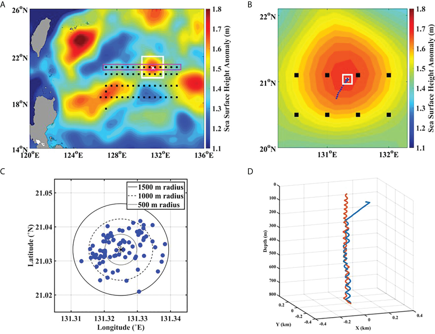
Figure 1 (A) Map of sea surface height (SSH) over the northwestern Pacific, including target spot (white cross in the white box), surrounded by warm and cold eddies of variable scale. The black dots indicate the path of R/V ISABU along which the conductivity–temperature–depth (CTD) profiles are obtained. Note that the eddy is approximately 1,000 km from the energetic region, Luzon Strait. (B) The white box of (A) is enlarged, where the SSH was obtained on September 11. A glider has moved to the eddy center along the path indicated by the blue dots. (C) The white box of (B) is enlarged. A glider was well controlled to surface within 720 m RMS around the waypoint, resulting in a dependable virtual mooring mode. (D) The underwater trajectory during a single dive of the Slocum glider attempting to hold the station at the target spot; dive (blue line) and climb (red line). Spiraling motion with a small radius is well maintained, except for the subsurface dive due to drift by the surface current.

Being restricted to a singular dataset obtained from a single Slocum glider inside a mesoscale eddy, any findings on the vertical structural variations of the DIT inside the eddy may be questionable. Thus, to see whether the vertical structure of ITs inside the eddy was significantly distinct from that outside the eddy, we performed a validation using the acoustic Doppler current profiler (ADCP) measurements obtained from R/V ISABU cruising outside the eddy for most of the cruise time (Figure 1A). Detailed descriptions of the dataset, measurements, and methods are provided in the following sections.

Methods

Glider

Gliders are slow-moving autonomous underwater vehicles that profile vertically by controlling buoyancy and moving horizontally on their wings (Rudnick et al., 2004). The mobility, high endurance, and relatively slow ascent/descent rate of gliders are appropriate for observing a variety of oceanic features with broad spatial extents but small vertical scales.

The glider used in this mission is a Slocum glider equipped with a Glider Payload CTD sensor and a Doppler Velocity Log (DVL) sensor. However, only CTD measurements were analyzed in this study, because the DVL sensor had been malfunctioned during the mission. The Slocum glider has a length of 2 m and hull diameter of 22 cm and typically weighs between 55 and 70 kg depending on its configuration; our glider weighed 65 kg. It is designed to run preprogrammed routes at depths ranging between 30 and 1,000 m. The glider on the surface regularly transmits real-time data via a satellite communication system to a ground station, through which the R/V ISABU (in this mission) receives the data and inversely transmits new instructions to the glider repeatedly. It steers through the water by controlling its pitch and heading via its rudder and can navigate between predetermined waypoints in a variety of oceanographic conditions, including swirling environments such as mesoscale eddies. Commanded remotely, gliders can acquire GPS position fixes and report their measurements via the Iridium satellite telephone while being at the sea surface level (at the end of each dive cycle).

Mesoscale anticyclonic eddy

A target eddy was selected as having a relatively circular shape, using the level 4 sea surface height (SSH) satellite data from the Copernicus Marine Environmental Monitoring Service (CMEMS: https://marine.copernicus.eu/access-data), which covered the R/V ISABU cruise route (see Figure 1A). The target eddy (white cross in Figure 1A and white box in Figure 1B) was located at 21.03°N and 131.25°E, approximately 1,000 km eastward from the Luzon Strait. According to the satellite-based observational work of Zhao (2014), DITs of K₁ and O₁ propagate over a long distance of approximately 2,500 km, indicating that DITs observed in this mesoscale eddy can be considered as coming from the Luzon Strait.

In order to compare the horizontal length scale of the target eddy with that of the first baroclinic diurnal internal tides in this area, we consider the parameter L_E as the length scale of the eddy following Dunphy and Lamb (2014). The L_E is computed via the horizontal structure function of the eddy $\text{ψ}\left(\text{r}\right)\sim \frac{5^{\frac{5}{2}}}{64}{U}_E{L}_{E}sec{h}^4\left(\frac{r}{L_E}\right),$ where r is a radial distance and U_E is a peak azimuthal velocity at $r=r_{max}=L_{E}tan{h}^{-1}\left(\sqrt{5}/5\right)\approx 0.48L_E$. In this study, the L_E of the target eddy is estimated to be about 192 km by fitting the horizontal structure function to the stream function from the SSH data (see Supplementary Figure S2B), and the r_max ~ 92km corresponds to the canonical eddy radius directly computed from the eddy velocity fields (not shown). Note that the eddy is not perfectly circular as shown in Figure 2; thus, the estimated diameter can be slightly different from the real one.

FIGURE 2

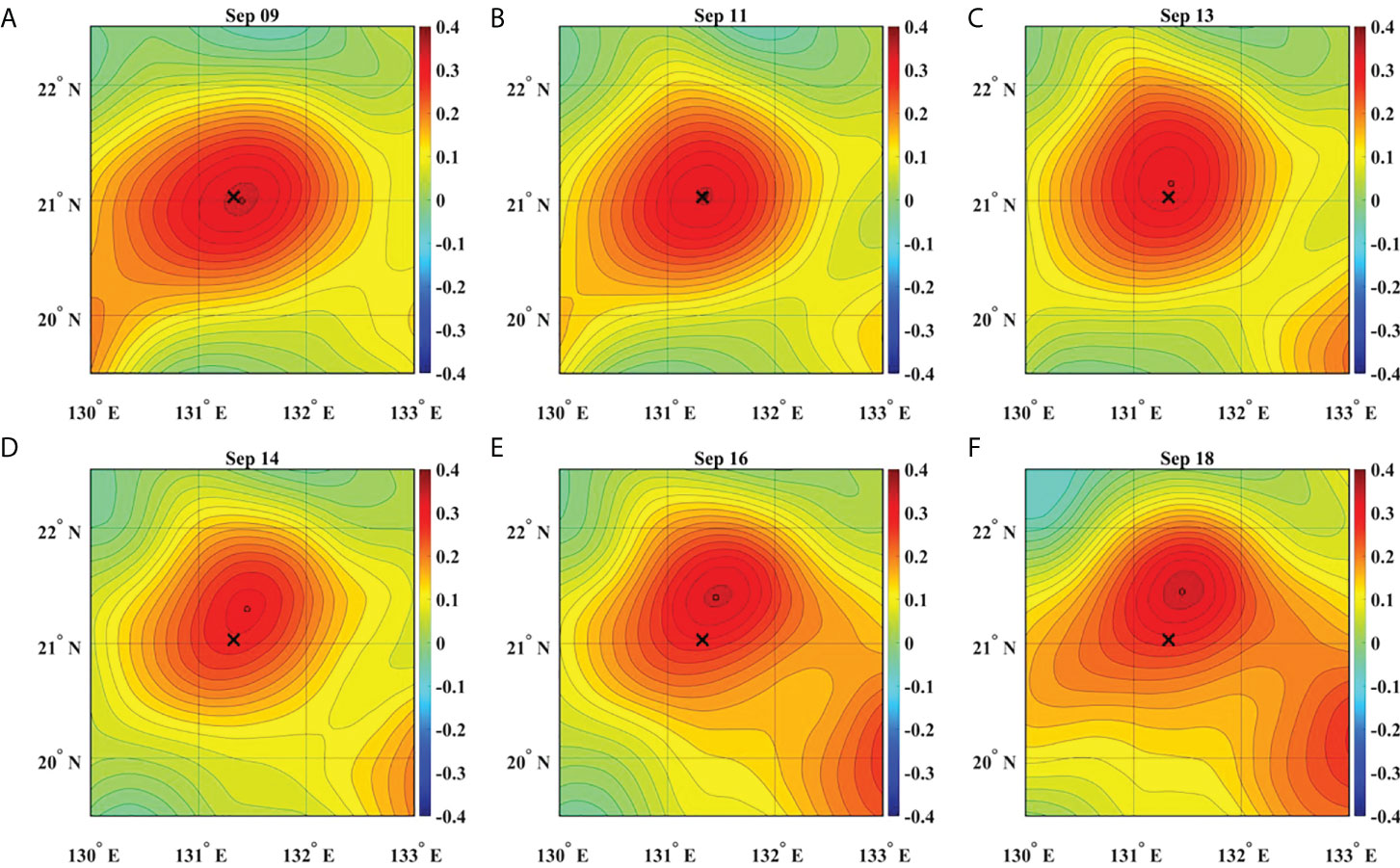
Figure 2 Contour map of SSHA satellite data (m), showing a moving mesoscale warm eddy during the VM glider measurement; the glider (black cross) scans near the inner center from September 9 to 13 (top panels, A through C), and near the outer center from September 14 to 18 (bottom panels, D through F).

During the glider’s VM profiling, the target eddy slowly traveled northward, as shown in Figure 2, where near-real-time satellite altimeter SSH and absolute geostrophic current data were displayed. Based on these satellite datasets, we calculated the relative vorticity from surface velocities computed based on geostrophic balance equations and the horizontal distance from the eddy center, as shown in Figure 3B. For comparison, we computed surface velocities based on a cyclo-geostrophic balance under the assumption of axis symmetry, but the differences between geostrophic and cyclo-geostrophic balances were small; the geostrophic velocities were underestimated by less than 10% (not shown). The relative vorticity shows a decreasing behavior in magnitude during the observation period, that is, depending on the distance from the eddy center, with a small hump between September 14 and 15. The relative vorticity shows a greater negative value in the region less than 30 km from the eddy center and a smaller negative value in the region greater than 30 km from the eddy center. For convenience, we call the area within the radius of 30 km from the eddy center as the inner center and the area of the circular ring with a radius of 30 to 50 km from the eddy center is called the outer center.

FIGURE 3

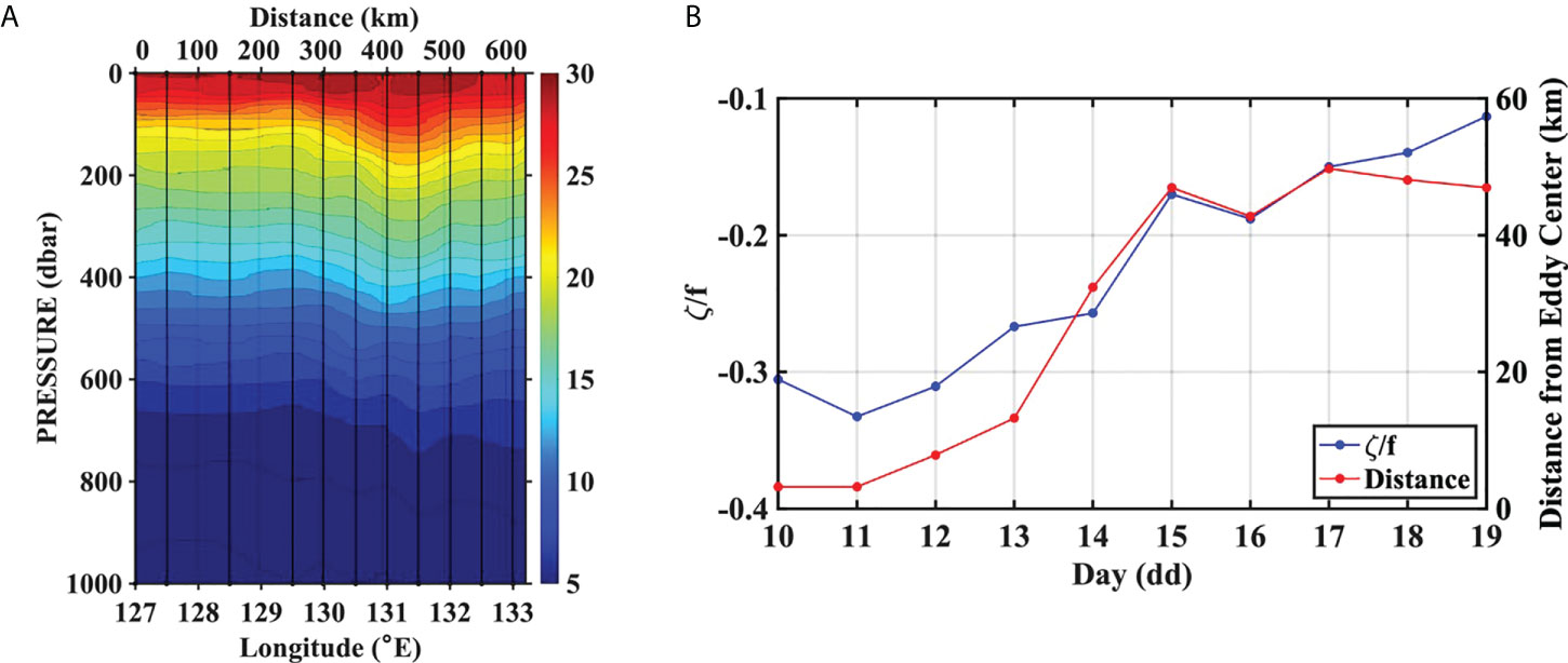
Figure 3 (A) The horizontal–vertical map of temperature variations along with isothermal curves obtained from CTD observations of the R/V ISABU represents the spatial structure of the eddy in the longitudinal range over approximately 130.5°E to 132.5°E; the bottom of the eddy reaches a depth of 400 m. (B) The vorticity at the glider position, calculated using satellite SSH data, is depicted along with distance from eddy center; a gradual increasing behavior of the vorticity with respect to the distance from the eddy center is noticeable, a slow increase in the former period (less than 30 km) vs. a fast increase in the latter period (more than 30 km).

As shown in Figure 3A, the isotherms show a convex pattern from the near surface to the depth of about 400 m, yet unclear eddy-like convex structures in the deeper layer, indicating that the mesoscale eddy has a baroclinic feature. This observation reveals that flow fields of the eddy may strongly affect the upper layer (shallower than 400 m), while weakly or negligibly affecting the lower layer (deeper than 400 m). Therefore, in the section of Available potential energy and horizontal kinetic energy, to compare the DIT energy levels between the upper and lower layers, we divide the whole observed water column (from the surface to 800-m depth) into the two layer, examining the DIT behaviors inside and outside of the eddy.

Glider measurement

A single Slocum glider was launched from the R/V ISABU at 20.71°N and 131.11°E on 8 September 2018 and actively traveled 42 km northward from the deployment site to the eddy center located at 21.03°N and 131.25°E through a predetermined route (blue dots in Figure 1B), while collecting CTD profiles by diving and climbing from the surface to 800-m depth in a sawtooth pattern. At the eddy center (the white box in Figure 1B), the glider was operated in virtual mooring mode from 10 to 19 September 2018, and it collected CTD profiles with a sampling frequency of 4 Hz, resulting in a vertical resolution of (average) 0.5 m. Only the CTD dataset obtained during this period was used in our study to examine the vertical structural variability of DIT inside the eddy. These CTD profiles have a high resolution in the vertical direction but a different temporal resolution at each depth, for example, from 1.4 h at the midpoint to 2.8 h at the top and bottom of the water column covered by the glider, because it takes an average of 2.8 h to complete one cycle (dive/climb). As shown in Figure 1D, the glider made a spiral motion with a small radius for a single dive/climb cycle, where the trajectory was estimated from the glider’s vertical velocity and heading information. When climbing, the glider usually drifts owing to background horizontal currents, resulting in the up-casts showing a better performance for the holding position than the down-casts (see Figure 1D). However, because there is no significant difference between gridded depth-time vertical displacements induced from the CTD dataset obtained by up-/down-casts and up-casts only (see Supplementary Figure S3), the CTD dataset by all casts (up/down) was used in this study.

The Slocum glider shows an enhanced station-keeping performance in VM mode, mainly because of its rudder-based steering, which makes a radius smaller than 20 m when changing the glider’s direction by 180°. This good performance yields a 720-m RMS of the glider’s surfacing spots from the waypoint (see Figure 1C and Supplementary Figure S4), where this dispersion is considered to be mainly due to the error in dead-reckoning navigation in the presence of internal tides near the study region and has almost no impact on vertical water properties with scales larger than several meters.

The migrating target eddy during VM profiling enables the glider to naturally scan the cross sections in the vicinity of the eddy center. Because it is important to trace the target eddy exactly for the goal of our study, we validated the locations of the eddy based on the satellite SSH anomaly contour map by comparing the satellite SSH anomaly and the dynamic height anomaly computed from the ISABU CTD dataset measured at the same location and during the period from September 4 to 7. As shown in Supplementary Figure S1, both data show good agreement, reaching a high Pearson cross-correlation value of R = 0.927. Also, the dynamic heights and SSH anomalies along the ship track are comparable to each other. (Supplementary Figure S2A).

Since September 4 before deployment of the glider, the anticyclonic eddy center shown in satellite SSH had been tracked and its location was predicted based on a simple linear extrapolation with the eddy translation velocity. The predicted location was determined as the glider VM position (21.03°N and 131.25°E). That was how the glider VM measurements could capture the variability in the vicinity of the eddy center (see Figure 3B).

Before analyzing the CTD samples measured by the glider, they were preprocessed via a smoothing procedure to eliminate a variety of measurement noises. They were gridded vertically at 1 m and temporally at 1-h resolution by linear interpolation; their size was 225 in time and 800 in depth. Then, a boxcar filter of 10 m vertically smoothed the gridded space–time series sufficiently to capture internal wave variations at diurnal and semidiurnal frequencies.

Shipboard measurements

The R/V ISABU traveled across the target eddy from 4 to 7 September 2018 (purple box in Figure 1A). During this period, CTD profiles were collected using a Sea-Bird Electronics (SBE) 911plus system. All instruments were calibrated before deployment, and the data were processed according to the manufacturer’s specifications. Measurements were obtained during up- and down-casts, but only the down-cast data were used to depict transects of temperature variability (Figure 3A) because Rosette bottle samples were made during the up-cast.

Since the glider observations are restricted on the eddy’s interior area, it is necessary to check out the DIT’s vertical structure outside the eddy. In order to compare the DIT’s variability inside and outside of the eddy (see the following section), we utilized the ADCP measurements collected from the R/V ISABU cruising outside the eddy from September 1 to 19, during which the route is indicated by black dots in Figure 1A. These horizontal current velocities were measured by a downward-looking 38-kHz ADCP over a water column of 50–800-m depths during the entire cruising period. The spatiotemporal variability of the internal tides can be aliased in the ADCP observations due to the irregular ship displacements over the sampling period; the zonal and meridional velocities by the shipboard ADCP are depicted in Figures 4A, B.

FIGURE 4

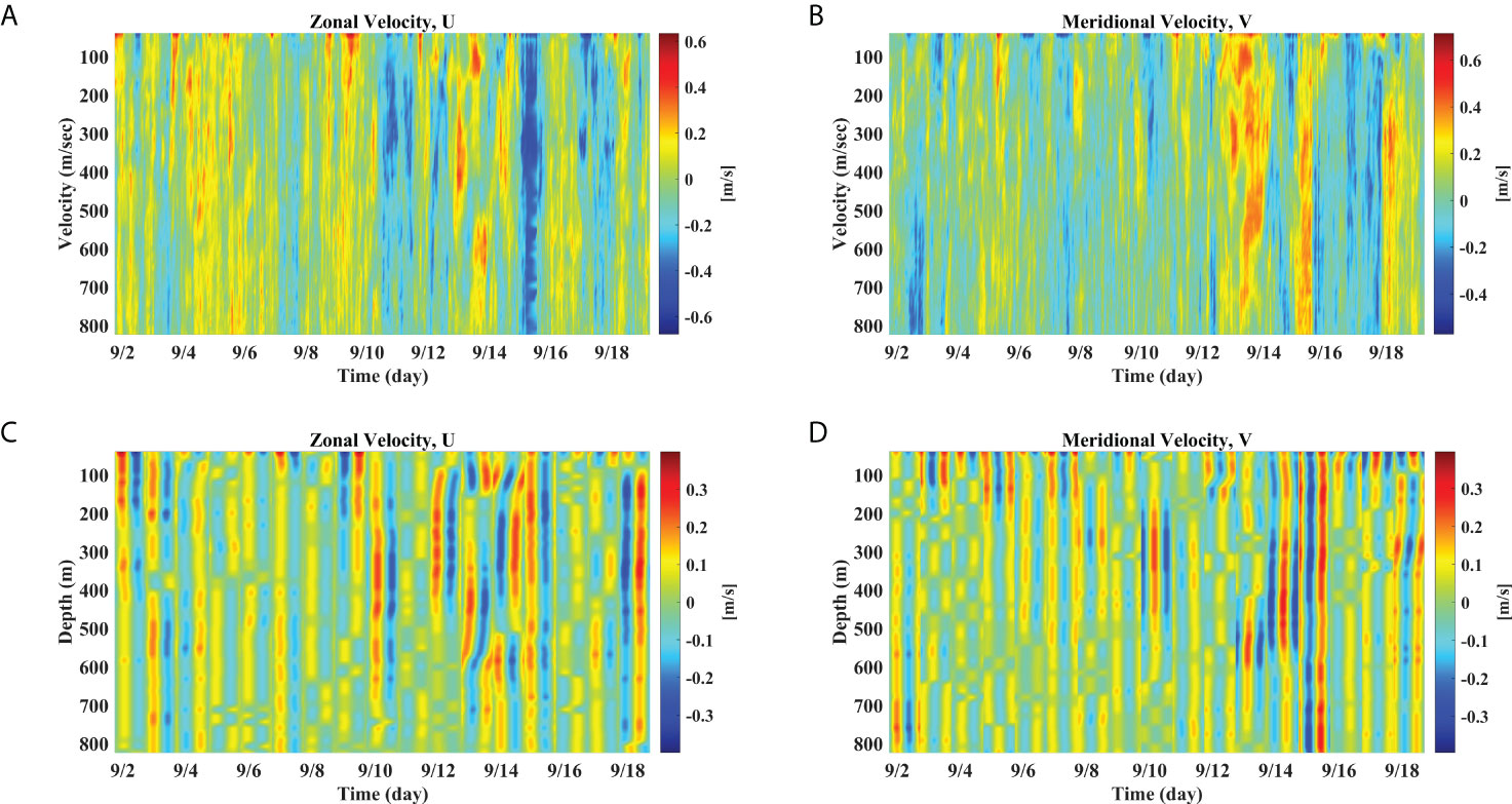
Figure 4 The depth–current profiles are presented, obtained from the cruising R/V ISABU during the period from September 1 to 19, including the interval of glider mission. The top panels (A) and (B) indicate the measured current velocities for zonal and meridional directions, respectively, while the bottom panels (C) and (D) are the mode-1 DIT fitted current profiles.

Estimating the mode-1 DIT current velocity

The ADCP data, obtained from the irregularly cruising R/V ISABU with on-average 3 m/s speed, are inappropriate for a direct isolation of ITs (DIT and SIT) via a standard bandpass filtering because they vary in space and time. Thus, we isolate the diurnal and semidiurnal ITs by applying a traveling sinusoidal model wave to ADCP measurements at each depth. According to the spectral analysis of vertical displacements estimated from the glider’s CTD measurements (see Figure 5B), DITs are observed to be dominant in isothermal vertical displacements. Thus, we estimated only the mode-1 DIT amplitude and phase via a least-square fit on a 1-day window after expressing the ADCP horizontal velocities of U and V as the following sinusoidal waves:

$\begin{array}{ll}\text{U}\left(\text{t},\text{z}\right)=U_{DIT}\left(z,t\right) sin\left(-{\omega }_{DIT}t+\overrightarrow{{\kappa }_h}·\overrightarrow{r}+{\phi }_U\left(\overrightarrow{r},z,t\right)\right)+\epsilon \left(t,z\right)& (1)\end{array}$

FIGURE 5

Figure 5 (A) The depth–time map of WKB-scaled isothermal displacements is depicted with isotherms corresponding to 29°C, 25°C, 20°C, 15°C, 10°C, and 6°C, where two white lines indicate 20°C and 10°C. (B) The power spectrums of vertical displacements of two isotherms correspond to 20°C (the upper layer) and 10°C (the lower layer), respectively. DIT dominates in the lower layer, whereas SIT is more pronounced in the upper layer rather than in the lower layer. (C) Diurnally band-passed isothermal displacements are depicted, showing a phase discrepancy between the upper and lower layers at the eddy center and gradually becoming in-phase away from the center. (D) Semi-diurnally band-passed vertical displacements show a complex pattern in magnitudes and phases.

and

$\begin{array}{ll}\text{V}\left(\text{t},\text{z}\right)=V_{DIT}\left(z,t\right) sin\left(-{\omega }_{DIT}t+\overrightarrow{{\kappa }_h}·\overrightarrow{r}+{\phi }_V\left(\overrightarrow{r},z,t\right)\right)+{\epsilon }^{\prime }\left(t,z\right),& (2)\end{array}$

where {U_DIT, V_DIT} and {ϕ_U,ϕ_V} are the amplitudes and phases of the sinusoidal DIT wave with K₁ (1/23.9345h^-1) frequency and mode-1 wavelength λ₁ (∼420km), which was computed via the phase speed C_p, under the influence of the Earth’s rotation, defined as

$\begin{array}{ll}{C}_p=\frac{\omega }{\sqrt{{\omega }^2-f^2}}C& (3)\end{array}$

where C is the eigenvalue speed obtained from the following eigenvalue equation (Gill, 1982)

$\begin{array}{ll}\frac{d^2\text{Φ}\left(z\right)}{d{z}^2}+\frac{N^2\left(z\right)}{C_n}\text{Φ}\left(z\right)=0& (4)\end{array}$

where the Brunt–Vaisala frequency profiles, N(z), are from climatological annual mean ocean stratification in the World Ocean Atlas 2018 (Locarnini et al., 2019; Zweng et al., 2019), and the mode number n = 1; hereafter, λ₁ = 420km is used.

In this estimation, we assumed that DITs travel only in the zonal direction and R/V ISABU travels at a constant day-averaged velocity (U_R/V,V_R/V) and thus $\overrightarrow{{\kappa }_h}=\left({\kappa }_x,{\kappa }_y\right)=\left(2\pi /{\lambda }_1\left(420km\right),0\right)$ and $\overrightarrow{r}=\left(x, y\right)=\left(U_{R/V }t,V_{R/V}t\right)$ were used in the above equations. The estimated mode-1 DIT current velocities are shown in Figures 4C, D.

To validate the above estimation method and evaluate the influence of propagation direction of ITs, we used a synthetic linear mode-1 DIT horizontal velocity with three propagation directions (0°, 30°,45°) with respect to the positive eastward direction, as a linear internal-wave solution under a constant stratification. The synthetic mode-1 DIT horizontal velocity based on a plane wave was generated using the following equations (Gill, 1982):

$\begin{array}{ll}u=-\frac{\pi }{{\kappa }_{1}H} cos\left(\frac{\pi z}{H}\right)sin\left({\kappa }_{1}x-{\omega }_{1}t\right)+ \eta \left(x,t\right),& (5)\end{array}$

$\begin{array}{ll}v=\frac{f}{{\omega }_1}\frac{\pi }{{\kappa }_{1}H} cos\left(\frac{\pi z}{H}\right)cos\left({\kappa }_{1}x-{\omega }_{1}t\right)+ \eta \left(x,t\right),& (6)\end{array}$

where f is the inertia frequency at latitude 21.03°N and (κ₁ω₁) denotes the wave number and frequency of a mode-1 DIT, with H = 5000m and with η (x,t) being a Brownian noise as a red noise. Using the R/V day-averaged cruising velocity records, we sampled the values from the synthetic (u,v) series. Supplementary Figures S5 A, B show synthetic mode-1 DIT current profiles, u and v, with red noise, and Supplementary Figures S5 C, D are the current velocities sampled by the cruising R/V ISABU; herein, a frequency-smearing due to Doppler effect induced by a traveling R/V is clearly observed. By applying Equations (1) and (2) to the sampled synthetic (u,v) series, mode-1 DIT estimates were obtained and depicted in Supplementary Figure S6, where a frequency-smearing is also clearly detected.

To examine the vertical structural variability of the DIT inside the eddy, we compared the vertical structural characteristics of the synthetic and estimated series in terms of the horizontal kinetic energy ratio (HKEr) defined in Equation (10). As shown in Supplementary Figure S7, there is no difference between them, where the estimated series has a nearly uniform value almost equal to the theoretical value of 0.5, indicating that the estimated mode-1 DIT velocity series accurately captures the vertical structural characteristics of the original series. In addition, the propagation directions of DIT have almost no impact on the vertical structure of the estimated velocity series (see Supplementary Figure S7B), although they yielded a slight variation in depth-integrated variance (see Supplementary Figure S6), implying that our estimation method (Equations 1 and 2) was robust to the IT propagation directions. However, it should be noted that the level of a red noise makes a significant impact on the vertical structure of the estimated velocity series (see Supplementary Figure S7B and Supplementary Figure S8B; the noise levels were set to be 10% and 100% of the velocity amplitude, respectively). The vertical structure seems to fluctuate more as the noise level increases. This point will be discussed in more detail in the section of Summary and discussion. Based on these simulation results, we characterized the vertical structure of the DIT outside the eddy using the mode-1 DIT velocity estimates from the ADCP measurements by the R/V ISABU.

Vertical displacement estimation

To investigate the behavior of the internal tides (DIT and SIT) inside the target eddy, we used the vertical displacements computed from the VM CTD measurements in the following analyses; we used the temperature only, and the raw temperature measurement by the glider is presented in Supplementary Figure S9, along with the temperature anomaly and the gridded temperature anomaly. The vertical displacement was calculated using $\text{η}\left(\text{z},\text{t}\right)=\left[T\left(z,t\right)-\overline{T}\left(z,t\right)\right]/\overline{T_z}\left(z,t\right)$, based on VM measurements. Here, T (z,t) denotes the gridded temperature measurements, and $\overline{T}\left(z,t\right)$ is the background temperature calculated by averaging T (z,t) over the entire observation period. The ${\overline{T}}_z\left(z,t\right)$ is the temperature gradient of $\overline{T}\left(z,t\right)$, that is, ${\overline{T}}_z\left(z,t\right)\equiv \partial \overline{T}\left(z,t\right)/\partial z$. From these gridded vertical displacements, we extracted internal tidal displacements (DIT and SIT) via fourth-order phase-preserving Butterworth bandpass filtering, with a central frequency of 1 cpd and half cpd with a bandwidth of 1/3 cpd, respectively.

Available potential energy and horizontal kinetic energy

In this study, DIT and SIT energies were computed following the procedure of previous studies (Zhao et al., 2010; Huang et al., 2018) and used to examine the vertical structure of ITs inside the eddy. Because only the VM glider CTD profiles are available for describing the characteristics of the ITs inside the eddy, the depth-integrated available potential energy (APE) is used to characterize the vertical structural variability of the DIT inside the eddy and is calculated as follows:

$\begin{array}{ll}APE\left(t\right)={\displaystyle {\int }_{-H}^{0}ape\left(z,t\right)dz=\frac{1}{2}}{\displaystyle {\int }_{-H}^0\langle \rho \left(z,t\right)N^2\left(z,t\right){\eta }^2\left(z,t\right)\rangle dz},& (7)\end{array}$

where ρ (z,t) denotes the water density calculated using TEOS 2010 (McDougall and Barker, 2011) from the CTD data, H denotes the water depth (here, the glider observation depth is used), the angle bracket denotes the average over one diurnal tidal cycle, and ape (z,t) is the spot APE. N² (z,t) is the squared buoyancy frequency calculated from the potential density smoothed by a 2-day sliding window. For the DIT and SIT, the corresponding displacements η (z,t) were isolated via bandpass filtering. To describe the vertical structural variability of ITs inside the eddy, we examined the vertical distributional pattern of APEs using the ratio of APE in the upper layer with respect to that in the whole water column (upper layer + lower layer), defined as follows:

$\begin{array}{ll}APEr\left(t\right)={\displaystyle {\int }_{-h}^0\langle \rho \left(z,t\right)N^2\left(z,t\right){\eta }^2\left(z,t\right)\rangle dz/{\displaystyle {\int }_{-H}^0\langle \rho \left(z,t\right)N^2\left(z,t\right){\eta }^2\left(z,t\right)\rangle dz}},& (8)\end{array}$

where h denotes the bottom depth of the upper layer, which was approximately 400 m. APEr is used to describe how the vertical structure of the DITs changes depending on the horizontal position inside the eddy.

As mentioned previously, any findings on the vertical structural variability of the DITs inside the eddy should be tested via comparison with those outside the eddy. To this end, we used the ADCP measurements from the R/V ISABU to describe the vertical structure of DITs outside the eddy in terms of the horizontal kinetic energy (HKE). The depth-integrated HKE is calculated as follows:

$\begin{array}{ll}\text{HKE}\left(\text{t}\right)={\displaystyle {\int }_{-H}^{0}hke\left(z,t\right)dz=\frac{1}{2}}{\displaystyle {\int }_{-H}^0\langle {\rho }_0{\left|{\overrightarrow{u}}^{\prime }\left(z,t\right)\right|}^2\rangle dz}& (9)\end{array}$

As in the case of APE inside the eddy, we define the ratio of HKE over depth to describe the vertical structural variability of IT outside the eddy, as follows:

$\begin{array}{ll}HKEr\left(t\right)={\displaystyle {\int }_{-h}^0\langle {\rho }_0{\left|{\overrightarrow{u}}^{\prime }\left(z,t\right)\right|}^2\rangle dz/}{\displaystyle {\int }_{-H}^0\langle {\rho }_0{\left|{\overrightarrow{u}}^{\prime }\left(z,t\right)\right|}^2\rangle dz}& (10)\end{array}$

where ${\overrightarrow{u}}^{\prime }$ is the baroclinic current computed by subtracting the depth-averaged current at each time from the measured current, and h is set to 400 m as done in APEr.

To equivalently compare the vertical structural characteristics of ITs inside and outside the eddy with different terms of APE and HKE, we have to convert HKE to APE. Although there is a well-known theoretical relation in which a progressive internal wave has a fixed HKE-to-APE ratio r_E=HKE/APE=(ω²+f²)/(ω²−f²) with ω being the tidal frequency and f being the inertial frequency, the ratio can be accurately obtained only during the full-depth integrations for HKE and APE, respectively, due to the wave reflections from the boundaries (bottom or surface) as discussed in Huang et al. (2018). However, it is not our goal to accurately estimate the ratio itself, but to compare the statistical tendency of the ratio in and out of the eddy. The vertical distributions of HKE and APE show a similar pattern (see FIG. B1 therein). Based on this behavior, APEr and HKEr are treated as a qualitative indicator showing the vertical structure of DIT energy distribution.

Wentzel–Kramers–Brillouin scaling

Typically, depth-varying stratification intensifies the horizontal velocity, energy density, and energy density flux near the surface, where stratification is strong, whereas isothermal displacements are amplified in deep water, where stratification is weak. Thus, to obtain a description of the vertical structural variability of ITs inside and outside the eddy without the complicated influence of variable stratification, all data were Wentzel–Kramers–Brillouin (WKB) normalized (Althaus et al., 2003). The appropriate scaling for the horizontal velocity is given as follows:

$\begin{array}{ll}\left(\widehat{\text{u}},\widehat{\text{v}}\right)=\left(\text{u},\text{v}\right)\sqrt{\frac{{\text{N}}_0}{{\overline{\text{N}}}_{\text{z}}}}& (11)\end{array}$

where the caret denotes the WKB-scaled value, $\overline{\text{N}}\left(\text{z}\right)$ is the time-mean measured buoyancy frequency, and N₀ = 7.40 × 10^-3s^-1 is a constant reference buoyancy frequency based on the depth-average buoyancy frequency, which is based on the VM CTD observations over the water column from the surface to a depth of 800 m.

The scaled vertical displacement is calculated as follows:

$\begin{array}{ll}\widehat{\text{η}}\left(\text{z},\text{t}\right)=\text{η}\left(\text{z},\text{t}\right)\sqrt{\frac{\overline{\text{N}}\left(\text{z}\right)}{{\text{N}}_0}}& (12)\end{array}$

The energy density scales are calculated as follows:

$\begin{array}{ll}\widehat{\text{E}}\left(\text{z},\text{t}\right)=\text{E}\left(\text{z},\text{t}\right)\frac{{\text{N}}_0}{{\overline{\text{N}}}_{\text{z}}}& (13)\end{array}$

where

$\begin{array}{ll}\text{E}\cong \text{HKE}+\text{APE}=\frac{\langle u^2+v^2\rangle }{2}+\frac{\langle N^2\left(z,t\right){\eta }^2\left(z,t\right)\rangle }{2}& (14)\end{array}$

and the angle brackets 〈 · 〉 denote an average over one diurnal tidal cycle.

The stretched-depth coordinate is calculated as follows:

$\begin{array}{ll}\widehat{\text{z}}={\displaystyle {\int }_z^0\frac{\overline{N}\left(z^{\prime }\right)}{N_0}d{z}^{\prime }}& (15)\end{array}$

In this stretched coordinate system, the bottom is shallower than that in reality. This scaling is equivalent to converting the ocean into a constant stratification, in which there is no spatial variability due to changes in stratification, and the vertical standing modes become sinusoids. In this study, the vertical column domain covered by the VM measurements corresponded to ~26% of the stretched water column, H_WKB = 3,100 m of the whole water column depth, and H = 5,000 m in the area near the target eddy. Therefore, although the glider observations were collected only at the top 800 m, they effectively sampled up to a quarter of the density range, enough to cover the eddy structure.

Results

Vertical displacements

The WKB-scaled isothermal vertical displacements are shown in Figure 5A, where six additional isotherms are plotted. The vertical displacement is distinctly intensified in the lower layer (deeper than 400 m) compared to that in the upper layer (shallower than 400 m) before September 14. Based on the SSH anomaly map (Figure 2) and the relative vorticity (Figure 3B), the glider can be regarded as residing in the inner center from September 10 to 14.

To compare the characteristics of vertical displacements in the upper and lower layers, we estimated the power spectral density (PSD) of 20°C and 10°C isothermal vertical displacements corresponding to WKB-scaled depths of 230 m (in the upper layer) and 550 m (in the lower layer), respectively, using PWELCH estimation of 50% overlapping segments with a size of 128. The power of DIT is certainly stronger in the lower layer than in the upper layer, and the relative power of DIT with respect to SIT is stronger in the lower layer (see Figure 5B). To examine the vertical structural variability of ITs inside the eddy, vertical displacements associated with DIT and SIT were isolated via fourth-order phase-preserving Butterworth bandpass filtering, with a central frequency at both 1 cpd and half cpd with a bandwidth of 1/3 cpd, respectively.

Viewed in band-passed DIT and SIT (see Figures 5C, D), the variational pattern of DIT inside the eddy is relatively clearer than that of SIT; DIT is stronger than SIT in intensity. The vertical structure of the DIT shows a noticeable variability in the inner center, that is, the intensity of vertical displacements seems to be focused on the lower layer (Figure 5C), as already confirmed in the spectral analysis, whereas SIT shows no distinct variability inside the eddy. This small-scale focusing behavior of DIT observed in the inner center could be partly due to wave–wave or wave–vortex interactions between the DIT and a mesoscale eddy. The significance of this behavior is addressed in terms of APE in the following section.

Lower-layer intensification of DIT vertical displacements inside the eddy

As confirmed by the vertical pattern of the DIT isothermal vertical displacements (see Figure 5C), small-scale focusing behavior was clearly observed only in the inner center. In this section, we describe the vertical structural variability of the DIT in terms of APE and APEr. The depth-integrated APEs for the three types of vertical displacements (total internal waves, DIT, and SIT) are first presented in Figure 6A, where a smooth up–down variation of APE in DIT might be partly due to a fortnight rhythm, although it is not entirely reliable because of the short duration of observation. The dominance of DIT over SIT inside the eddy was reconfirmed in terms of APE. Second, APEr reconfirms the small-scale focusing behavior of DIT in the inner center as shown in Figure 5C. Although limited to the inside of the eddy, the vertical structure of the DIT appears to differ between the inner and outer centers (see Figure 6B). However, for the SIT, there seems to be a distinct behavior inside the eddy but its behavior is not as dramatic as compared to DIT. Thus, we performed an analysis only on DIT in the following sections; concerning not analyzing SIT, we give some plausible reasons in the section of Summary and discussion.

FIGURE 6

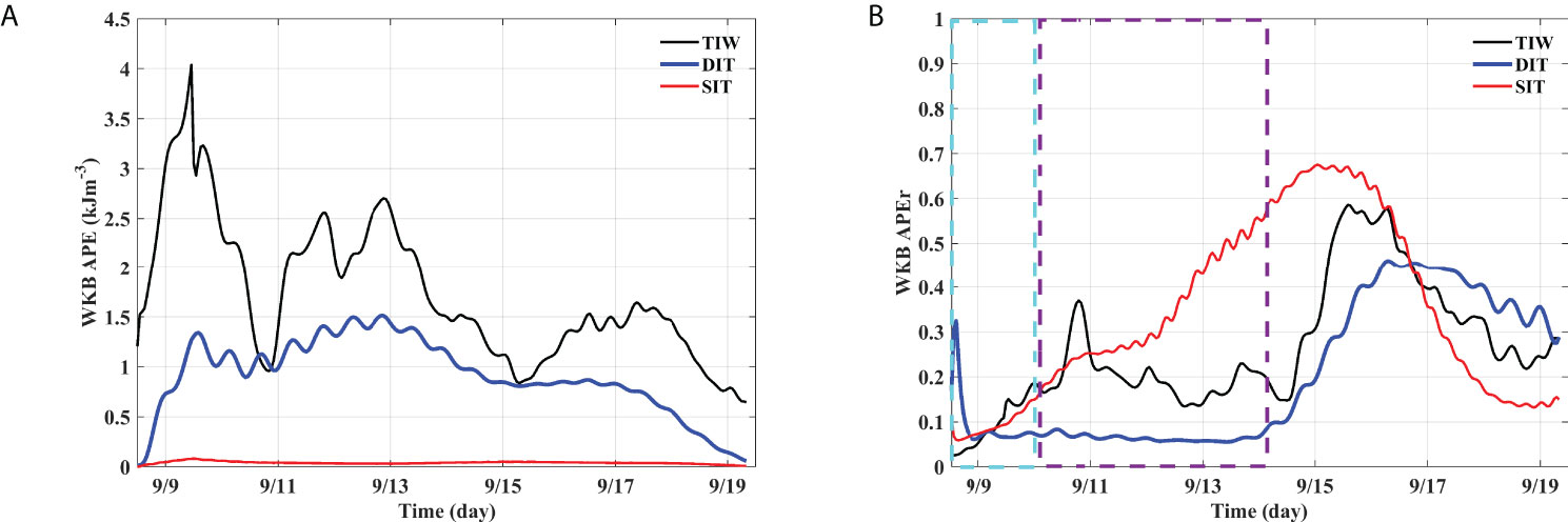
Figure 6 The available depth-integrated APEs are shown. (A) APEs of total internal waves (TIW), DIT, and SIT are shown for the entire glider observation period. (B) APE ratios (APEr) of the upper layer to the entire water column are plotted during the same period. A cyan broken-line box denotes the pre-VM interval during which the glider moves in a zig-zag manner to a target station, and the purple box denotes the eddy center (target) under VM measurements.

The small-scale focusing behavior of DIT may be an intermittent ocean feature in ocean environments outside the eddy. Thus, we must validate that this behavior is significantly different from the usual oceanic features observed in ocean environments without mesoscale eddies. To this end, we estimated the mode-1 DIT current velocity from the R/V-mounted ADCP measurements obtained outside the target eddy via Equations (1) and (2) and examined the vertical structural variability of the mode-1 DIT in terms of HKEr using these estimates. Figures 4A, B show the horizontal velocity obtained from the traveling R/V-mounted ADCP, where we can see the phase modulation, as already confirmed in the case of synthetic DIT signals. Figures 4C, D show the estimated mode-1 DIT current velocity, from which HKE and HKEr are computed. Figure 7A shows the varying HKE over depth and time, and HKEr is presented in Figure 7B. Based on the argument in the section of Available potential energy and horizontal kinetic energy, we qualitatively interpret the behavior of HKEr similar to that of APEr. First, a slight convex curve in the red broken-line box is observed; the time span corresponds to the period during which the R/V ISABU traveled across near the eddy center. This slight convexity appears to be associated with the dramatic focusing behavior of DIT shown in Figure 6B; however, there is another possibility related to the background noise. Likewise, the more fluctuating behavior observed in the time span of September 10–14 may be related to two factors, interaction and background noise (see Figure 7B). These observational behaviors are discussed in more detail in the section of Summary and discussion. Second, the overall range of values of HKEr is limited to [0.5, 0.7] when neglecting the time span of September 10–14. Based on these results, it seems natural that the small-scale focusing behavior observed in the inner center is a distinct feature that is only observed inside of the inner center. Thus, it can be said that this focusing behavior is linked to some type of interaction between DITs and a mesoscale eddy.

FIGURE 7

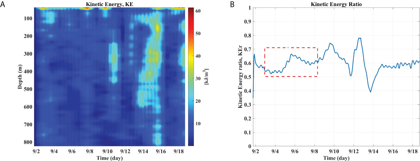
Figure 7 The horizontal kinetic energy (HKE), computed from the mode-1 fitted current estimates, is presented in (A), and the ratio of HKE of the upper 400 m with respect to the whole column down to 800 m is plotted in (B). The red broken-line box in (B) indicates the time span during which the ISABU traveled across the target eddy’s center. Also, compared to the ratio of APE within the eddy, the behavior of HKEr is clearly distinguished. Note that HKE and APE are linearly dependent via a linear internal wave theory.

Low-mode energy transferring behavior of DIT inside the eddy

Energy transfer between the vertical modes of internal waves via their interaction with mean fields and mesoscale eddies, such as resonant triad interactions (McComas and Bretherton, 1977), is a critical energy-cascading mechanism that dissipates large-scale energy into smaller scales, leading to various vertical mixings.

A direct investigation of energy cascades among vertical modes is possible in numerical simulation experiments, as done in the work of Dunphy and Lamb (2014), where a single coherent SIT was incident on the synthetic eddy of length scales comparable to those of an incoming SIT; the comparability in scales of ITs and mesoscale eddies is important to enhance the conversion efficiency from mode-1 to mode-2 or higher. Most in situ measurements obtained from physical mooring platforms provide reliable results on low-to-high modal conversion via a modal decomposition, since there are small gaps in the top and bottom of the water column. However, it is usually impossible to obtain reliable results on the energy cascading behavior from glider-based measurements because they have large bottom gaps; in this study, the water column covered by the glider was 800 m with respect to the full depth of 5,000 m and a modal decomposition is not possible to the limited vertical extent of the observations (Nash et al., 2005). Owing to this limitation, we take an indirect qualitative approach to obtain any clues about the energy transferring behavior among low vertical modes occurring inside the eddy, which has already been confirmed as a small-scale focusing behavior. For diurnally band-passed 1-h gridded vertical displacements (DIT) during the entire observation, the vertical wavenumber spectral estimates were computed every hour (1 h), from which the lowest four vertical wavenumbers (K_z (1) ~ K_z (4)) were selected every hour (1 h), and their power spectral densities (PSDs) were averaged over 24 h in a non-overlapping manner. The 24-h summed spectral powers of K_z (1) and K_z (2) are presented in Figure 8A, where the K_z (1) spectral power behaves like a fortnight IT rhythm and the ratio of K_z (2) with respect to K_z (1) shows a meaningful behavior. This behavior of K_z (2)/ K_z (1) ratio seems to indicate that the modal conversion from K_z (1) to K_z (2) is more active in the inner center than in the outer center. When extended to the four lowest wavenumbers, the K_z (2 ~ 4)/ K_z (1) ratio showed a consistent behavior (see Figure 8B). This characteristic behavior can be a qualitative clue to the energy transfer from low-to-high mode occurring among low vertical modes, being strong in the inner center and weak in the outer center.

FIGURE 8

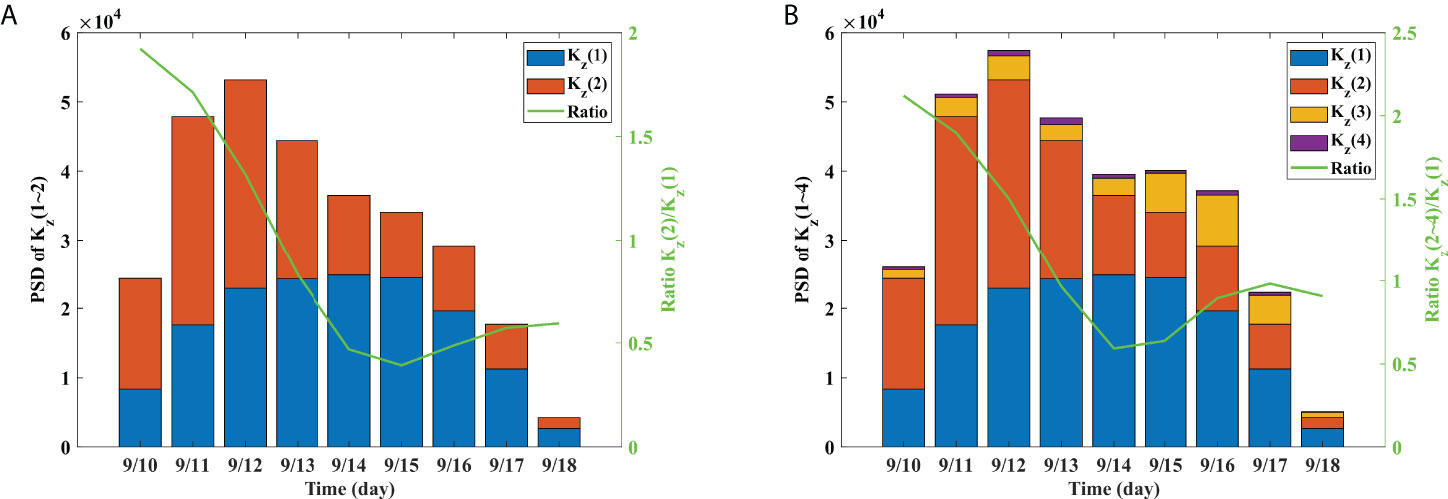
Figure 8 The 24-h averaged PSDs of vertical DIT wavenumbers are shown. (A) PSDs of the lowest two vertical wavenumbers are plotted over the virtual mooring duration, along with the ratio (right y-axis). (B) PSDs of the lowest four vertical wavenumbers are plotted, along with the ratio.

Summary and discussion

In this study, the vertical structural variability of the DIT inside a mesoscale anticyclonic eddy was examined based on VM CTD measurements obtained from a single Slocum glider. The Slocum glider actively traveled 42 km northeastward from the R/V ISABU along the predetermined route to the center of a target mesoscale (blue dots in Figure 1B), where VM observation was performed for approximately 10 days (~225 h) from 10 to 19 September 2018. During the VM observation, the eddy slowly migrated northward about 50 km (see Figure 2 and the red line in Figure 3B), which enabled the glider to scan the cross sections inside the eddy.

Because gliders typically travel a distance of 20 to 30 km per day, the flight mode observation by a glider is inadequate to capture the oceanic processes inside the eddy core, such as vertical structural variability of internal tides (DIT and SIT) in a small-scale region of less than 50 km, as in this study. Therefore, a well-controlled VM approach was adopted. In this study, the Slocum glider showed excellent performance for maintaining its station while collecting CTD profiles inside the target eddy, resulting in surfacing within 720-m RMS from the waypoint, as shown in Figure 1C. This point is more evident in comparison with the position-keeping performance of the ocean station PAPA (see Supplementary Figure S4). The Slocum glider’s good station-keeping performance is mainly due to two factors: a high-frequency spiraling motion with a small radius and a motion with a smaller radius (less than 20 m) motion made by rudder-based steering when changing its direction by 180°. In addition, to reduce any possible Doppler effect induced by the glider’s motion, we applied bandpass filtering with wider widths around tidal frequencies to the gridded dataset with a temporal resolution of 1 h and vertical resolution of 1 m.

The VM observations based on this performance successfully captured the variability of ITs (DIT and SIT) inside the eddy and detected the small-scale focusing behavior of DIT appearing in the inner center (less than 30 km in the horizontal), which is well described in terms of isothermal vertical displacements (see Figure 5C). An ideal measurement to capture the DIT structure inside the eddy center might be to make several gliders follow the eddy; however, it is difficult to keep those gliders at certain locations relative to the translating eddy center because their horizontal speeds are difficult to precisely control in the presence of varying background currents.

The intensified vertical displacement of DIT in the lower layer is also captured in the frequency spectral analysis (Figure 5B) of the vertical displacements of the two isotherms at 20°C (the upper layer) and 10°C (the lower layer); the spectral power of the DIT is stronger in the lower layer than in the upper layer. In addition, a peak in the PSD was clearly observed at the diurnal frequency for both layers, indicating that DITs dominantly contributed to vertical displacements inside the eddy. This observation seems to be in contrast with the glider-based observational study (Rainville et al., 2013), where DIT and SIT energy fluxes with similar intensities were observed to propagate into the Western Pacific near the Luzon Strait. However, this noticeable weakness of SIT against DIT inside the eddy seems to be partly consistent with satellite altimeter observations (Zhao, 2014), where M2 appears to be more refracted equatorward than K1 near the location of our target eddy, although there is still no plausible explanation. Also, DIT is more coherent than SIT near the eddy as shown in the phase of internal tide elevations based on MIOST-IT products (see Supplementary Figures S10 C, D and Supplementary S11 C, D). This point coincides with observations in Zhao (2014) where K1 and O1 internal tides have one source (Luzon Strait) but M2 internal tides originate from the Luzon Strait and the Ryukyu Ridge, whose amplitudes are significantly small compared to K1 internal tides.

The focusing behavior of DIT as an indicator of DIT’s vertical structural variability was qualitatively reconfirmed in terms of APEr (see Figure 6B), indicating that DIT experienced a stronger vertical structural change in the inner center than in the outer center. This location-dependent behavior is not due to the stratification of the water column because there is no clear difference in stratification between the inner and the outer centers (see Supplementary Figure S12); the stratification is another indicator for the refraction of internal tides (Zaron and Egbert, 2014). However, there remains a critical pitfall in arguing that this finding is distinctly an eddy-specific feature because the VM observation is restricted to the region with a small horizontal scale of approximately 50 km inside the eddy. Thus, to test whether the focusing behavior detected inside the eddy was significantly different from the usual modulations of DITs due to background mean fields without mesoscale eddies, we examined the vertical structural variability of mode-1 DIT using mode-1 DIT velocity estimates computed via our estimation method (Equations 1 and 2) from ADCP measurements by R/V ISABU, which traveled over a wide area including our study region (black dots in Figure 1A denote the R/V route during the mission) from September 1 to 19.

The estimation method was firstly tested on a synthetic linear mode-1 velocity series contaminated with a Brownian noise with a 10th level of amplitude of mode-1 velocity. The aliasing and smearing in frequency and amplitude due to the measurements by a traveling vehicle are clearly visible especially in two time spans September 4–6 and September 10–14 (Supplementary Figure S5 and Supplementary Figure S6). The vertical structure of horizontal kinetic energy looks stable over the whole observation duration irrespective of propagation directions of DITs and the traveling behavior of R/V ISABU under the low level of background noise (Supplementary Figure S7B); however, fluctuations in the vertical structure are observed in two time spans September 4–6 and September 10–13 when the noise level increases to that of mode-1 velocity (Supplementary Figure S8B). It should be noted that these fluctuations seem to be not due to the interaction between internal tides and background mean fields but due to the dependency of estimation method on background noise levels. These results imply that the fluctuations observed in Figure 7B during September 10–13 could be due to the presence of background noise and are therefore better to be excluded for estimating the background structure of DIT. Also, the red broken-line box in Figure 7B should be more cautiously interpreted. A slight convex curve is observed in the red broken-line box, possibly indicating that a vertical structural variability of DIT occurs. The slightness of a convex curve in the red broken-line box can be explained from two perspectives. One is the fluctuating behavior by the presence of background noise (red noise) when estimating the mode-1 DIT velocity signals. This behavior seems to be mainly due to the traveling pattern of R/V ISABU such as an abrupt change of velocity (see Supplementary Figure S13, therein the results are based on 20 synthetic DIT signals). The large deviation of HKEr values in the time span of September 10–13 implies strongly that the corresponding time span should be excluded when estimating the vertical structure of DIT outside the eddy. The other is that the R/V ISABU passed through the eddy region ~30 km from the eddy’s center point during September 5–7 (see Supplementary Figure S14), implying that the DIT’s focusing behavior in the inner center might not be clearly captured by the ISABU.

When excluding the two durations of September 4–6 and September 10–13, the HKE in the oceanic environment outside the eddy seems to be mainly concentrated in the upper layer, giving an on-average HKEr value of 0.6, which is definitely different from the APEr value of less than 0.1 in the inner center. Based on the assumption of similarity in behaviors of APE and HKE in the water column, the observed small-scale focusing behavior in the inner center (less than 30 km on a horizontal scale) can be said to be an eddy-specific feature.

Based on this focusing behavior observed in the inner center, we considered the energy transfer occurring between the vertical modes of the internal waves. Several mechanisms have been theoretically investigated and well established (Polzin and Lvov, 2011) for energy cascading processes in the wavenumber–frequency domains. In particular, the cascading process in vertical wavenumbers between two internal equal-frequency waves is well explained for wave–wave–vortex triad interactions (Lelong and Riley, 1991). According to the numerical work of Dunphy and Lamb (2014), the incoming SIT exhibits a cascading process from low to high modes in vertical dynamic modes and frequencies (harmonics) after passing through a mode-1 baroclinic mesoscale eddy.

To examine energy-cascading processes, a traditional dynamic vertical-mode approach is typically utilized. However, because our VM glider observations are restricted to the upper 800-m depth from the surface, this dynamic-mode approach is inapplicable. Instead, as an indirect approach, we examined the temporal variations of the vertical wavenumber spectra of the diurnally band-passed vertical displacements, which were computed at every gridded time and averaged over 24 h in a non-overlapping manner. From the day-based wavenumber power spectra of DIT, the lowest four wavenumbers K_z (1)~ K_z (4) were selected as proxies for the low vertical modes. As shown in Figures 8A, B, the ratios of spectral power of K_z (2) and K_z (2) ~ K_z (4) with respect to that of K_z (1) show a dramatic variation over time, that is, depending on the horizontal positions inside the eddy. These characteristic behaviors imply that the energy transfer occurring among low vertical modes is strong at the inner center and weak at the outer center. It should be noted that the four lowest vertical wavenumbers are not corresponding in a one-to-one manner to vertical mode-1 through mode-4 of DIT passing through the eddy. The varying power spectral density of K_z (1) ~ K_z (4) represents the variation of energy density in low modes of DITs.

There is a noticeable coincidence in the patterns observed in the relative vorticity (Figure 3B), small-scale focusing behavior of DIT (Figures 5C, 6B), and transfer behavior of the lowest four wavenumbers of DIT (Figures 8A, B). These observational findings seem to have implications for the interaction between DIT and a mesoscale eddy, including resonant triad interactions among wave–wave–vortices. According to the work of Lelong and Riley (1991), the wave–vortex triad predicts the resonant or near-resonant interaction of a mode-1 wave of tidal frequency with a periodic mode-1 baroclinic vortex field of zero frequency, which is expected to generate a mode-two wave of tidal frequency. Rainville and Pinkel (2006) observed the increasing incoherence of the energy flux during the eddy periods via a shift of the propagation path of the individual modes, which increases with mode numbers. Dunphy and Lamb (2014) found that the energy conversion efficiency of SIT from mode-1 to modes 2 and higher reaches a maximum of 13% for eddies with a diameter of 60 km (2L_E) when interacting with the mode-1 SIT of 76.1-km horizontal wavelength at latitude of 20N in terms of absolute power loss, the loss curve was peaked for eddies with a diameter of near 70 km (2L_E). This numerical finding strongly supports the importance of having comparable length scales in both eddies and low-mode internal tides. In our study, the horizontal scale of mode-1 DIT was approximately 420 km, and the diameter of the target eddy was about 400 km. This fact indicates that the scattering of the mode-1 DIT rather than SITs within the eddy is very probable, which is in good agreement with our observational findings, whereas SIT’s vertical structural variability is less dramatic compared to that of DIT (Figure 6B). Also, the incoherence in SIT (see Supplementary Figures S11 C, D) reduces the performance of mode-1 SIT velocity estimation from the R/V ISABU ADCP measurements via a plane wave fitting (Equations 1 and 2), so we cannot test whether the variability of SIT in Figure 6B is temporal variation usually observed outside the eddy.

In addition, our observations seem to be related to the findings of Chavanne et al. (2010), in which two numerical results based on 3D ray tracing were presented and qualitatively consistent with observations on the impact of energetic surface-intensified mesoscale currents, a cyclone of 55-km diameter and ~100-km vertical decay scale, as well as vorticity waves of ~100-km wavelength and 100–200-m vertical decay scale, on the propagation of M₂ internal tides with a horizontal wavelength of 50 km and vertical wavelength of 0(1,000 m); the semidiurnal surface currents were obtained by high-frequency radars and moored ADCPs. In their numerical results, a mesoscale cyclone caused the energy of internal tide rays propagating through its core to increase near the surface, and vorticity waves enhanced or reduced the energy near the surface depending on their phases. Compared to their descriptions of the variability of M₂ internal tides (current profiles) within a cyclonic eddy, we present a similar behavior of DIT (vertical displacements) inside an anticyclonic eddy, along with a local vorticity dependency of the variability of the DIT’s vertical structure.

Consequently, our observational findings imply that two factors seem to play a critical role in the intensity of interactions between internal tides and mesoscale eddies: one is the comparability of horizontal scales of eddies and internal tides, confirmed in the numerical study of Dunphy and Lamb (2014), and the other is the relative vorticity inside the eddy, similarly revealed in the work of Chavanne et al. (2010). However, our claim should be considered with caution because these results were based on a spatiotemporally restricted dataset. Thus, two tasks are urgent to give more concrete observational basis and to reveal the underlying mechanism. The first thing is that multiple-glider VM observations with longer durations and wider scopes are required to make a concrete claim on the relationship between the vertical structural variability of the DIT and the relative vorticity. The second thing is to make an appropriate numerical study, since the interaction between internal wave and baroclinic eddy is known as a non-trivial and non-linear process.

Data availability statement

The altimeter products were produced by SSALTO/DUACS and distributed by Aviso+ with support from Cnes (https://www.aviso.altimetry.fr). The MIOST-IT products were designed, implemented and validated by CLS, OCEAN-NEXT and LEGOS and distributed by Aviso+ (https://www.aviso.altimetry.fr) with support from Cnes.

Author contributions

JJP conceptualized the study and collected samples; JJP and GL contributed equally to data analysis; GL contributed to writing the draft; JJP revised the final manuscript. All authors contributed to the article and approved the submitted version.

Funding

This research was a part of the project titled “Development of the core technology and establishment of the operation center for underwater gliders,” funded by the Ministry of Oceans and Fisheries, Korea (1525012198). This research was also supported by Kyungpook National University Development Project Research Fund, 2021.

Acknowledgments

The authors acknowledge the help of BongJoon Kim, YunChang Kwak, and the KAOS (Center for Korea Autonomous Ocean observing System) team in the Glider operation. We also sincerely acknowledge Dr. Sok-Kuh Kang and the crews of R/V ISABU for their warm cooperation during the hydrographic measurements of cruises.

Conflict of interest

The authors declare that the research was conducted in the absence of any commercial or financial relationships that could be construed as potential conflict of interest.

Publisher’s note

All claims expressed in this article are solely those of the authors and do not necessarily represent those of their affiliated organizations, or those of the publisher, the editors and the reviewers. Any product that may be evaluated in this article, or claim that may be made by its manufacturer, is not guaranteed or endorsed by the publisher.

Supplementary material

The Supplementary Material for this article can be found online at: https://www.frontiersin.org/articles/10.3389/fmars.2022.920049/full#supplementary-material

References

Alford M. H. (2003). Redistribution of energy available for ocean mixing by long-range propagation of internal waves. Nature 423, 159–162. doi: 10.1038/nature01628

CrossRef Full Text | Google Scholar

Alford M. H., Mickett J. B., Zhang S., MacCready P., Zhao Z., Newton J. (2012). Internal waves on the Washington continental shelf. Oceanography 25, 66–79. doi: 10.5670/oceanog.2012.43

CrossRef Full Text | Google Scholar

Althaus A. M., Kunze E., Sanford T. B. (2003). Internal tide radiation from mendocino escarpment. J. Phys. Oceanogr. 41, 2211–2222. doi: 10.1175/1520-0485(2003)033<1510:ITRFME>2.0.CO;2

CrossRef Full Text | Google Scholar

Bühler O., Mclntyre M. E. (2005). Wave capture and wave-vortex duality. J. Fluid. Mech. 534, 67–95. doi: 10.1017/S0022112005004374

CrossRef Full Text | Google Scholar

Chavanne C., Flament P., Luther D., Gurgel K.-W. (2010). The surface expression of semidiurnal internal tides near a strong source at Hawaii: Part II: Interactions with mesoscale currents. J. Phys. Oceanogr. 40, 1180–1200. doi: 10.1175/2010JPO4223.1

CrossRef Full Text | Google Scholar

Dunphy M., Lamb K. G. (2014). Focusing and vertical mode scattering of the first mode internal tide by mesoscale eddy interaction. J. Geophys. Res. Ocean. 119, 523–536. doi: 10.1002/2013JC009293

CrossRef Full Text | Google Scholar

Egbert G. D., Ray R. D. (2000). Significant dissipation of tidal energy in the deep ocean inferred from satellite altimeter data. Nature 405, 775–778. doi: 10.1038/35015531

CrossRef Full Text | Google Scholar

Gill A. (1982) Atmosphere-ocean dynamics (Elsevier Science). Available at: https://www.perlego.com/book/1828147/atmosphereocean-dynamics-pdf (Accessed 25 September 2021).

Google Scholar

Huang X., Wang Z., Zhang Z., Yang Y., Zhou C., Yang Q., et al. (2018). Role of mesoscale eddies in modulating the semidiurnal internal tide: Observation results in the northern south China Sea. J. Phys. Oceanogr. 48, 1749–1770. doi: 10.1175/JPO-D-17-0209.1

CrossRef Full Text | Google Scholar

Kelly S. M., Lermusiaux P. E. J. (2016). Internal-tide interactions with the gulf stream and middle Atlantic bight shelfbreak front. J. Geophys. Res. 121, 6271–6294. doi: 10.1002/2016jc011639

CrossRef Full Text | Google Scholar

Kerry C. G., Powell B. S., Carter G. S. (2014). The impact of subtidal circulation on internal tide generation and propagation in the Philippine Sea. J. Phys. Oceanogr. 44, 1386–1405. doi: 10.1175/JPO-D-13-0142.1

CrossRef Full Text | Google Scholar

Lelong M. P., Riley J. J. (1991). Internal wave-vortical mode interactions in strongly stratified flows. J. Fluid. Mech. 232, 1–19. doi: 10.1017/S0022112091003609

CrossRef Full Text | Google Scholar

Löb J., Köhler J., Mertens C., Walter M., Li Z., von Storch J.-S., et al. (2020). Observations of the low-mode internal tide and its interaction with mesoscale flow south of the Azores. J. Geophys. Res. 125, e2019JC015879. doi: 10.1029/2019JC015879

CrossRef Full Text | Google Scholar

Locarnini R. A., Mishonov A. V., Baranova O. K., Boyer T. P., Zweng M. M., Garcia H. E., et al. (2019). World ocean atlas 2018, volume 1: Temperature. Mishonov A., Technical Editor. NOAA Atlas NESDIS, 52pp.

Google Scholar

McComas C. H., Bretherton F. P. (1977). Resonant interaction of oceanic internal waves. J. Geophys. Res. 82, 1397–1412. doi: 10.1029/JC082i009p01397

CrossRef Full Text | Google Scholar

McDougall T. J., Barker P. M. (2011). Getting started with TEOS-10 and the Gibbs seawater (GSW) oceanographic toolbox, 28pp., SCOR/IAPSO WG127, ISBN 978-0-646-55621-5.

Google Scholar

Munk W., Wunsch C. (1998). Abyssal recipes II: Energetics of tidal and wind mixing. Deep. Sea. Res. I. 45, 1977–2010. doi: 10.1016/S0967-0637(98)00070-3

CrossRef Full Text | Google Scholar

Nash J. D., Alford M. H., Kunze E. (2005). Estimating internal wave energy fluxes in the ocean. J. Atmos. Ocean. Technol. 22, 1551–1570. doi: 10.1175/JTECH1784.1

CrossRef Full Text | Google Scholar

Nash J. D., Kelly S. M., Shroyer E. L., Moum J. N., Duda T. F. (2012). The unpredictable nature of internal tides on continental shelves. J. Phys. Oceanogr. 42, 1981–2000. doi: 10.1175/JPO-D-12-028.1

CrossRef Full Text | Google Scholar

Polzin K. L., Lvov Y. V. (2011). Toward regional characterizations of the oceanic internal wavefield. Rev. Geophys. 49, RG4003. doi: 10.1029/2010RG000329

CrossRef Full Text | Google Scholar

Rainville L., Lee C. M., Rudnick D. L., Yang K. C. (2013). Propagation of internal tides generated near Luzon strait: Observations from autonomous gliders. J. Geophys. Res. 118, 4125–4138. doi: 10.1002/jgrc.20293

CrossRef Full Text | Google Scholar

Rainville L., Pinkel R. (2006). Propagation of low-mode internal waves through the ocean. J. Phys. Oceanogr. 36 (6), 1220–1236. doi: 10.1175/jpo2889.1

CrossRef Full Text | Google Scholar

Rudnick D. L., Davis R. E., Eriksen C. C., Fratantoni D. M., Perry M. J. (2004). Underwater gliders for ocean research. Mar. Technol. Soc J. 38 (2), 73–84. doi: 10.4031/002533204787522703

CrossRef Full Text | Google Scholar

Tian J., Zhou L., Zhang X., Liang X., Zheng Q., Zhao W. (2003). Estimates of M2 internal tide energy fluxes along the margin of northwestern pacific using TOPEX/POSEIDON altimeter data. Geophys. Res. Lett. 30, 1889. doi: 10.1029/2003GL018008

CrossRef Full Text | Google Scholar

Villamana M., Carballido B. M., Maranon E., Cermeno P., Choucino P., da Silva, et al. (2017). Role of internal waves on mixing, nutrient supply and phytoplankton community structure during spring and neap tides in the upwelling ecosystem of ria de vigo (NW Iberian peninsula). Limnol. Oceanogr. 62, 1014–1030. doi: 10.1002/lno.10482

CrossRef Full Text | Google Scholar

Whalen C. B., Talley L. D., MacKinnon J. A. (2012). Spatial and temporal variability of global ocean mixing inferred from argo profiles. Geophys. Res. Lett. 39, L18612. doi: 10.1029/2012GL053196

CrossRef Full Text | Google Scholar

Wunsch C., Ferrari R. (2004). Vertical mixing, energy, and the general circulation of the oceans. Ann. Rev. Fluid. Mech. 36, 281–314. doi: 10.1146/annurev.fluid.36.050802.122121

CrossRef Full Text | Google Scholar

Zaron E. D., Egbert G. D. (2014). Time-variable refraction of the internal tide at the Hawaiian ridge. J. Phys. Oceanogr. 44 (2), 538–557. doi: 10.1175/jpo-d-12-0238.1

CrossRef Full Text | Google Scholar

Zhao Z. (2014). Internal tide radiation from the Luzon strait. J. Geophys. Res. 119, 5434–5448. doi: 10.1002/2014JC010014

CrossRef Full Text | Google Scholar

Zhao Z., Alford M. H., MacKinnon J. A., Pinkel R. (2010). Long-range propagation of the semidiurnal internal tide from the Hawaiian ridge. J. Phys. Oceanogr. 40, 713–736. doi: 10.1175/2009JPO4207.1

CrossRef Full Text | Google Scholar

Zweng M. M., Reagan J. R., Seidov D., Boyer T. P., Locarnini R. A., Garcia H. E., et al. (2019). World ocean atlas 2018, volume 2: Salinity. A. Mishonov, Technical Editor, NOAA Atlas NESDIS 82, 50pp.

Google Scholar