Mixing in the upper western equatorial Pacific driven by westerly wind event

Diapycnal mixing in the upper western equatorial Pacific (WEP) plays an important role in the tropical air–sea interactions and in the formation of the global climate system. Yet, the WEP is uniquely rich in water masses originating from the two hemispheres and in multiscale processes of different dynamical nature, thus creating a complex regime of mixing remains to be fully characterized by elaborate observations. Here, on the basis of microstructure measurements in the WEP, we report the observations on a strong deep cycle turbulence extending well into the upper thermocline by westerly wind event, with the turbulent kinetic energy dissipation rate ε~O(10⁻⁸–10⁻⁷) W kg⁻¹ and diapycnal diffusivity K_ρ∼O(10⁻⁴) m² s⁻¹. Below the deep cycle turbulence layer, turbulence and mixing are generally weak with ε~O(10⁻¹⁰–10⁻⁹) W kg⁻¹ and K_ρ∼O(10⁻⁷–10⁻⁶) m² s⁻¹, a prototype of the weak mixing nature of the low-latitude western Pacific. The observed turbulence below the deep cycle turbulence layer can be satisfactorily scaled by either the MacKinnon–Gregg model or the Richardson number–based model with tuned model parameters.

1 Introduction

The variability of the upper ocean heat content and ocean circulation in the western equatorial Pacific (WEP) is closely connected to zonal displacements of the western Pacific warm pool and the associated air–sea interactions and, therefore, the global climate system, including particularly the El Niño and Southern Oscillation (ENSO). Diapycnal mixing is assumed to play a critical role in these processes through redistributing heat, salt, and momentum across the isopycnals (Philander and Pacanowski, 1980). A thorough understanding of the spatiotemporal variation of diapycnal mixing and its driving mechanisms in the WEP is therefore an important objective of the current oceanographic and climatic research.

The wind forcing and surface buoyancy fluxes at the air–sea interface are the main factors controlling mixing processes in the upper mixed layer. In contrast, mixing processes occurring in the ocean interior away from the boundaries remain poorly understood. Conventionally, diapycnal mixing in the ocean interior is thought to be generated by the breaking of internal waves and/or shear instability of currents. The microstructure measurements along three meridional transects over 5°S–5°N of the WEP suggest that thermocline mixing over 50–250 m is mostly associated with small-vertical-scale velocity shear structures, with the turbulent kinetic energy (TKE) dissipation rate (ε) of 10⁻¹⁰–10⁻⁸ W kg⁻¹ and the diapycnal diffusivity (K_ρ) of 10⁻⁶–10⁻⁴ m² s⁻¹ (Richards et al., 2012; Richards et al., 2015). Furthermore, such thermocline mixing has interannual variability due to the changes in stratification during the ENSO events. Microstructure measurements along two orthogonal transects across the Mindanao eddy (Liu et al., 2017) revealed that thermocline mixing is generally weak with ε of O(10⁻¹⁰) W kg⁻¹ and K_ρ of O(10⁻⁶) m² s⁻¹ due to reduced internal wave breaking at low latitudes (Henyey et al., 1986; Gregg et al., 2003), but is enhanced with K_ρ one order of magnitude larger at the eddy flanks due to geostrophic shear. On the basis of the two 3-day intensive microstructure measurements in the WEP, Liu et al. (2022) reported strong turbulence and diapycnal mixing in the halocline-induced barrier layer with ε of O(10⁻⁸–10⁻⁶) W kg⁻¹ and K_ρ of O(10⁻⁵–10⁻³) m² s⁻¹. Microstructure measurements over 0–10°N of the WEP suggested that enhanced mixing with K_ρ of O(10⁻⁴) m² s⁻¹ occurs below the thermocline over 250–750 m due to weakened stratification induced by the South Pacific Tropical Water (SPTW) intrusion (Liang et al., 2019). Earlier microstructure observations suggest weak diapycnal diffusivity of O(10⁻⁵) m² s⁻¹ at deeper depths of 1,000–1,600 m over 0–20°N of the WEP (Hibiya et al., 2007). In addition to these microstructure measurements, there are also indirect estimates of diapycnal mixing in the WEP. On the basis of long-term finescale velocity measurements, Zhang et al. (2018; 2019) proposed that enhanced mixing is present over 0–2°N due to intensified vertical shear of zonal currents and can also occur in anticyclonic subthermocline eddies due to strong sub-inertial velocity shear and weakened stratification associated with the eddies.

These previous studies have greatly advanced our understanding of diapycnal mixing in the WEP, but it is based on very limited measurements with contrasting implications. Furthermore, the WEP runs at the crossroads of different water masses where they converge and exchange their properties (Tsuchiya et al., 1989; Fine et al., 1994; Kaneko et al., 1998). The WEP is also influenced by various atmospheric forcing, such as easterly trade winds and westerly wind events (WWEs), and entails rich dynamical processes, such as vertically and horizontally alternating westward and eastward zonal currents, swift and narrow western boundary currents, as well as surface and subsurface mesoscale eddies. These processes dynamically modulate the stratification, shear, and mixing, and therefore, more measurements are needed to better define mixing characteristics and variabilities in the WEP. To this end, we conducted microstructure measurements in the WEP.

2 Data and methods

Field observations were conducted at 16 stations roughly along 1–3°N from 138°E to 152°E during 17–28 December 2018 (Figure 1). Microstructure data were obtained with a free-falling tethered Vertical Microstructure Profiler (VMP500, Rockland Scientific International Inc.), which was equipped with two fast shear probes, two FP07 thermistors, and one SBE7 micro-conductivity probe. The sampling frequency was 512 Hz. The VMP500 was released at the windward side of the boat. The typical descending speed rates were ~0.5 m s⁻¹. The maximum depth of the casts varied from 372 to 750 m due to different weather and oceanographic conditions. At each station, only one cast of the VMP500 was made due to limited ship time.

FIGURE 1

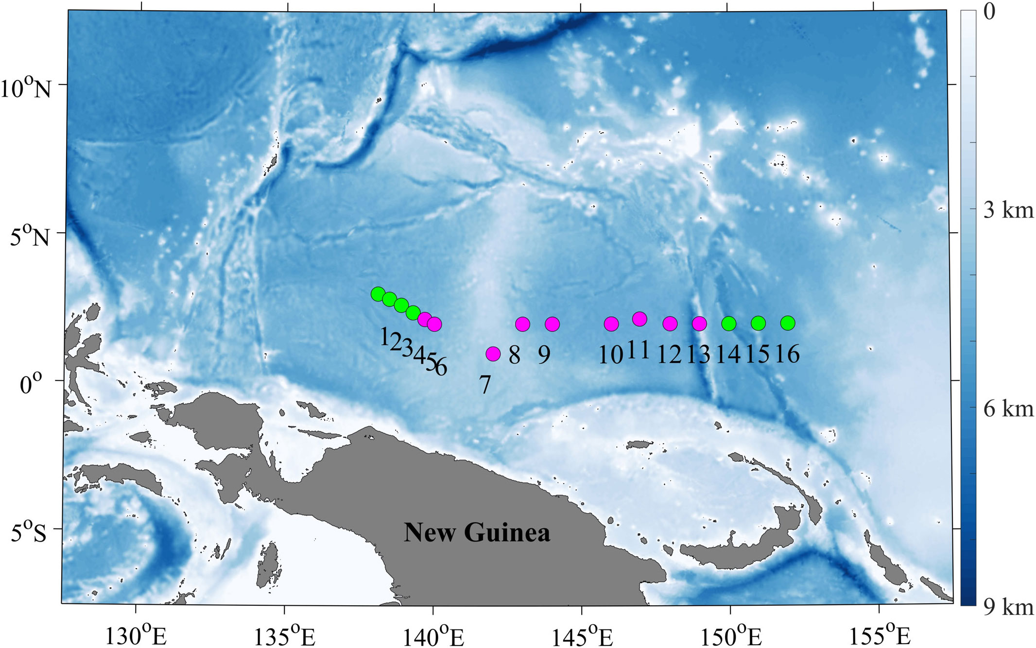
Figure 1 The locations of measurement stations with color shading denoting the topography (ETOPO1) in the western Pacific Ocean. Magenta and green denote the stations with and without the presence of deep cycle turbulence (DCT), respectively.

The microstructure data processing followed the procedures described in the technical note (Lueck, 2016). The raw shear data were first de-spiked to remove anomalous data spikes. The profile of microscale shear was divided into consecutive half‐overlapping 8-s segments, roughly corresponding to a vertical bin size of ~4 m. In each segment, the value of ε was calculated by fitting the theoretical Nasmyth spectrum to the measured shear spectra. Shear spectra Φ(k) computed from the shear signals are shown by the red and blue curves in Figures 2A–D along with the corresponding scaled Nasmyth universal spectra (black curves; Nasmyth, 1970). The shape of the measured spectra agrees well with the universal spectrum except in the high wavenumber regions affected by vibration noise (Wolk et al., 2002). To further quantify their agreement, we calculated the mean absolute deviation (MAD) between the observed (S_obs) and theoretical (S_th) spectra: $\text{MAD = }\frac{1}{n}\sum _0^{k_u}\mid \frac{S_{obs}}{S_{\mathit{th}}}-<\frac{S_{obs}}{S_{\mathit{\text{th}}}}>\mid$, where k_u is the upper wavenumber limit and n is the number of wavenumber values. Following the criterion of Ruddick et al. (2000), the data segment with MAD larger than 2(2/d)^1/2 was rejected, where d = 26 is the freedom. Figure 2E shows the example of MAD profilers at Station 16. For all stations, only 1% of data segments were rejected. The 96% of the ratios between two estimates of ε from the two shear probes were within a factor of 5. Under such a condition, two estimates of ε were averaged. Otherwise, we used the estimate of ε with a smaller value (Vladoiu et al., 2019). The estimated ε values over 0–5 m were excluded due to the contamination of the ship’s wake.

FIGURE 2

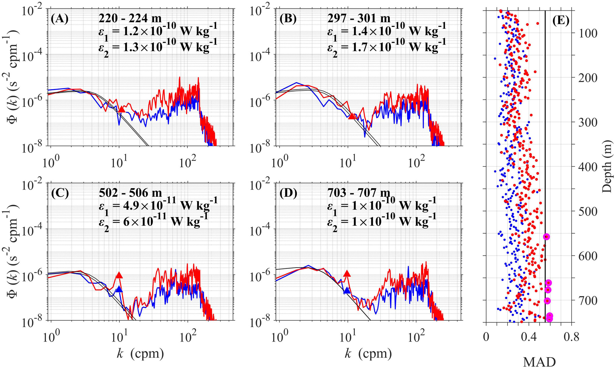
Figure 2 (A–D) Observed and theoretical Nasmyth (black) shear spectra over different depth ranges, and (E) vertical profiles of mean absolute deviation (MAD) of the spectral values between observed and Nasmyth spectra over the integration wavenumber range at Station 16 as an example. In panels (A–D), the triangles indicate the upper wavenumber limits of integration. In panel (E), the black line denotes the rejection limit of MAD (see text), and magenta circles indicate the data segments with MAD larger than the rejection limit. Data from two shear probes are denoted in blue and red, respectively.

Vertical profiles of salinity, temperature, and pressure were measured with a shipboard Sea-Bird 911 plus conductivity-temperature-depth (CTD). The CTD data were post-processed to account for time lags between the temperature and conductivity sensors, for the thermal mass of the conductivity sensor, and to remove pressure inversions due to ship rolling. Then, the temperature and salinity data were averaged into 1-m bins. The squared buoyancy frequency (N²) was computed from density according to N² = −(g/ρ) ∂ρ/∂z based on the observed temperature and salinity.

Velocity profiles were measured with a set of (one upward-looking and one downward-looking) TRDI (Teledyne RD Instruments) lowered acoustic Doppler current profilers (LADCPs) attached to the water sample rosette. Both the upward- and downward-looking LADCPs were operated at 300 kHz with a 10-m bin size. The LADCP profiles were processed using an inversion method based on the LDEO software (Visbeck, 2002). Velocity profiles were collected using 1 ping per ensemble with ensemble sampled at 1 Hz during downcast and upcast, and were then jointly constrained by bottom-tracking velocity, ship drift data from GPS, and upper-ocean velocities measured by a 38 kHz shipboard ADCP. The shear variance, S² = (∂u/∂z)² + (∂v/∂z)², was calculated by first-differentiating zonal and meridional velocities (u and v) over a 10-m interval.

To reduce the bias introduced by the different vertical resolutions of N² and S², N² was smoothed by 10-m running mean vertically. Values of N², S², and ε were then interpolated into 1 m to calculate the Richardson number and the diapycnal diffusivity. The Richardson number was obtained by Ri = N²/S². The value of diapycnal diffusivity was estimated on the basis of the Osborn relationship, i.e., K_ρ = 0.2 ε/N², in which a canonical value of 0.2 of the mixing efficiency was adopted (Osborn, 1980).

3 Results

3.1 Mixing associated with westerly wind event

The microstructure measurements experienced substantially different wind forcing. On the basis of the data from the shipboard Vaisala automatic weather station, the wind speed at 10-m height above the sea surface (U₁₀) increased from ~5–7 m s⁻¹ at Stations 1–4 to ~12 m s⁻¹ at Station 11, and then decreased to ~2 m s⁻¹ at Station 16 (red line in Figure 3A). ASCAT (Advanced Scatterometer) wind speed (black line in Figure 3A) and direction (figure not shown) show similar values and variations. We further examine the longitude-time evolution of ASCAT zonal wind stress anomalies over 2018–2019. From 16 to 30 December 2018, a WWE occurred over 120–160°E (Figure 3C). The WWE is defined as the equatorial regions in the 5°S–5°N band with zonal wind stress anomalies greater than 0.05 N m⁻² over 10° longitude and lasting more than 5 days (Menkes et al., 2014). Thus, the observed intensified wind belongs to this WWE. Next, we discuss the responses of turbulence in the surface mixed layer and in the stratified water well below the surface mixed layer to WWE. The base of the surface mixed layer is defined as the depth where the potential density (σ_θ) change is 0.01 kg m⁻³ from the measured lowest density (MacKinnon and Gregg, 2005).

FIGURE 3

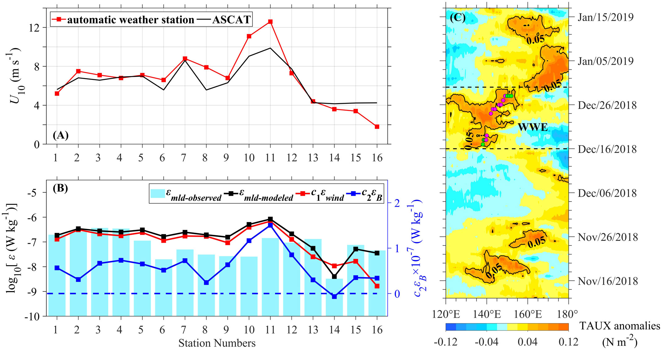
Figure 3 Station series of (A) wind speed at 10-m height above the sea surface (U₁₀) from shipboard Vaisala automatic weather station (red) and ASCAT (black), and (B) mean TKE dissipation rates over the mixed layer from observation (ε_mld-observed, bar charts), model (ε_mld-modeled, black), and its two components induced by wind (ε_wind, red) and convection (ε_B, blue). (C) Longitude-time variation of ASCAT zonal wind stress (TAUX) anomalies averaged over 5°S–5°N with measurement stations indicated. The westerly wind event (WWE) is denoted by two horizontal dashed black lines.

The surface mixed layer was gradually deepened from 20 to 60 m from Stations 1 to 16 (thick solid line in Figure 4). The value of N² in the mixed layer was at least one order of magnitude smaller than shear variance (Figures 4C, D). This led to the value of Ri falling below 0.25, corresponding to the occurrence of strong turbulence and diapycnal mixing with ε > 10⁻⁸ W kg⁻¹ and K_ρ> 10⁻⁴ m² s⁻¹, respectively (Figures 4E–G). The TKE dissipation rates induced by wind stress (ε_wind) and buoyancy flux-related convection (ε_B) are mainly two sources of mixed layer turbulence. The observed TKE dissipation rate (ε_mld-observed) can be scaled by ε_mld-modeled = c₁ε_wind + c₂ε_B, where c₁ = 1.76 and c₂ = 0.58 are proportionality constants (Lombardo and Gregg, 1989). The value of ε_wind is calculated by ε_wind = 1/κz(τ_w/ρ₀)^3/2, where κ = 0.4 is von Karman’s constant, z is depth, ρ₀ = 1021 kg m⁻³ is the mean water potential density in the mixed layer, and τ_w is wind stress computed from the observed U₁₀. The TKE dissipation rate induced by convection is obtained by ε_B = J_B, where J_B is surface buoyancy flux. The value of J_B was calculated following the procedure from Shay and Gregg (1986), using the observed U₁₀, air temperature and pressure, sea-level pressure, and relative humidity from shipboard Vaisala automatic weather station, observed surface potential temperature (θ) from CTD, and net shortwave radiation, albedo, and cloud cover from ECMWF (European Centre for Medium-Range Weather Forecasts) ERA-interim. The positive sign of J_B indicates a net buoyancy loss of the upper ocean, which facilitates mixing due to convection. In general, the mean value of ε_mld-modeled over the mixed layer reasonably depicts that of ε_mld-observed in variation with a correlation of 0.6 at the 95% confidence level and in size within the same order of magnitude (Figure 3B). This suggests that this scaling can be applicable to the WEP. When the wind speed rates were very weak at Stations 13 and 15–16, the value of c₂ε_B accounts for 73% of ε_mld-modeled on average, suggesting that the buoyancy flux made a great contribution to the mixed layer turbulence. Note that c₂ε_B at Station 14 was negative, corresponding to the restratification process. When the value of U₁₀ was larger than 5 m s⁻¹ at Stations 1–12, the value of c₁ε_wind accounts for 74% of ε_mld-modeled on average, suggesting that the wind frictional stress is a major contributor to turbulence in the mixed layer (Figures 3A, B).

FIGURE 4

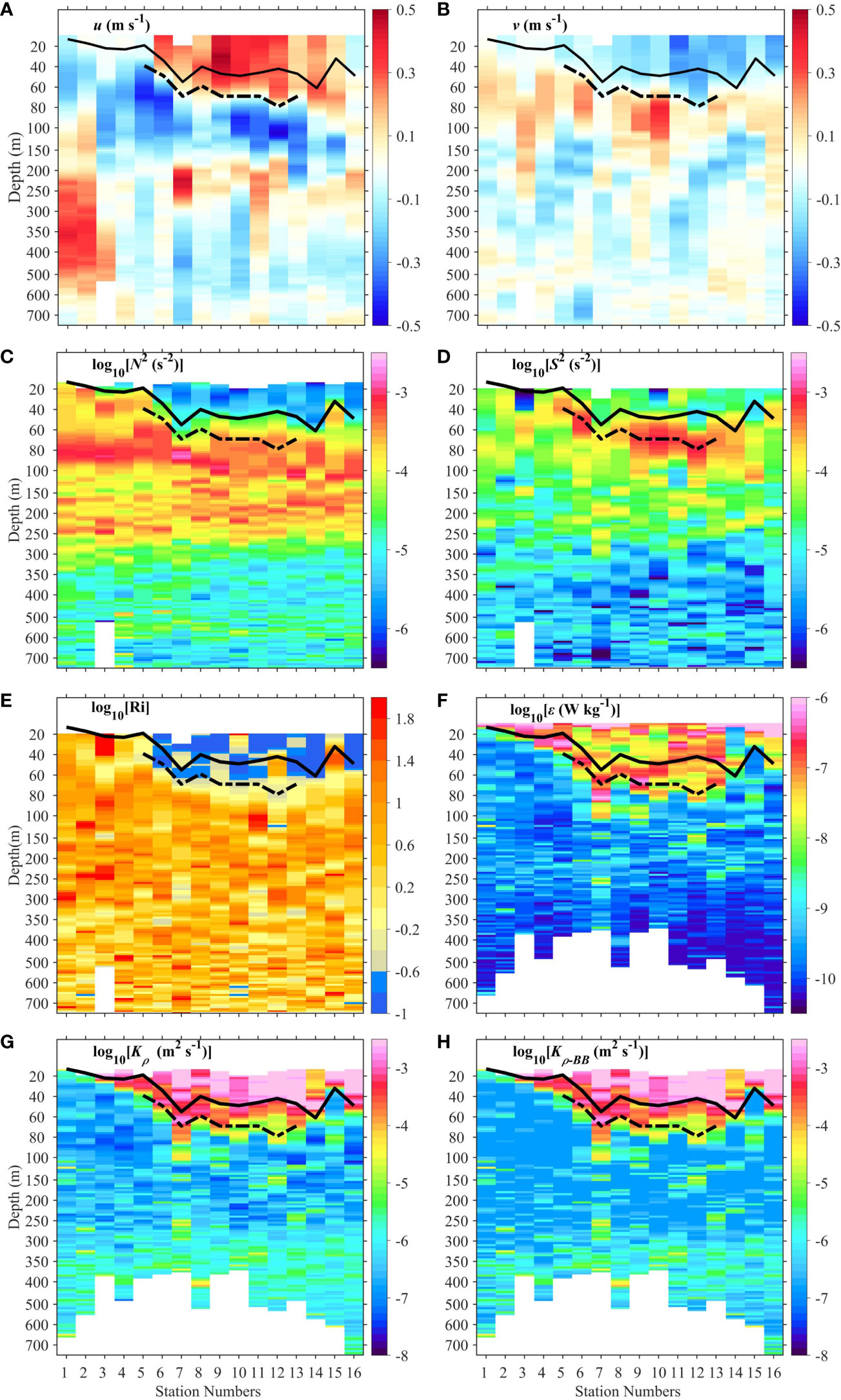
Figure 4 Depth-station variations of observed (A) zonal velocities (u), (B) meridional velocities (v), (C) squared buoyancy frequency (N²), (D) shear variance (S²), (E) Richardson number (Ri), (F) TKE dissipation rate (ε), and (G) diapycnal diffusivity calculated from Osborn relationship (K_ρ) and (H) from Bouffard and Boegman (2013; K_ρ-BB). The thick solid and dash-dotted lines indicate the bases of the mixed layer and the deep cycle turbulence layer, respectively. Note that the y-axis is not uniform.

In addition to the surface mixed layer, the WWE can further exert an influence on the stratified water well below the mixed layer. At Stations 1–4, the westerly wind speed was relatively weak, and the South Equatorial Current (SEC) occupied the upper 100-m depth. With WWE intensifying at Stations 5–13, the westerly wind caused gradually increasing eastward velocity in the mixed layer, and this eastward current depressed the westward flowing SEC to 20–30 m below the base of the mixed layer (Figure 4A). This led to strong shear and small Ri near the interface depth of two zonal currents, resulting in larger ε (Figures 4D–F). This strong turbulence extended well into the stably stratified waters from the base of the mixed layer to the depth of the maximum S² (between the thick solid and dash-dotted lines in Figure 4). Note that the zonal velocity primarily caused the strong shear here, and the meridional velocity had little contribution (Figures 4A, B). When the westerly wind calmed down again at Station 14–16, the surface current gradually reversed into the westward direction, and the strong turbulence below the mixed layer vanished. The measurement stations can be divided into two ensembles, including the strong turbulence occurring ensemble (Stations 5–13) and the background ensemble without the presence of the strong turbulence (Stations 1–4/14–16).

Figure 5 shows the vertical profiles of ensemble-mean S², Ri, ε, K_ρ, and turbulent heat flux (J_q) around the surface mixed layer and their 95% bootstrapped confidence intervals. The strong turbulence at Stations 5–13 is similar to the “deep cycle turbulence” (DCT), initially and widely observed in the eastern equatorial Pacific Ocean (Gregg et al., 1985; Moum and Caldwell, 1985). Their similarities include that both are presented at the depth well below the mixed layer and that both correspond to a marginal instability with Ri fluctuating around 0.25 (Figure 5B and Table 1; Thorpe and Liu, 2009; Smyth and Moum, 2013) and therefore strong turbulence with ε~O(10⁻⁸–10⁻⁷) W kg⁻¹ and K_ρ~O(10⁻⁴) m² s⁻¹, at least one to two orders of magnitude larger than the background ensemble values (Figures 5C, D and Table 1). For convenience, we hereafter still use DCT to refer to such strong turbulence below the mixed layer, although the diurnal cycle of DCT was not captured due to the lack of continuous measurement. The DCT occurred in a scenario with relatively high diffusivity and thermal gradient. This resulted in strong turbulent heat flux from the base of the mixed layer into the ocean interior, with important implications for the climate (e.g., Moum et al., 2013; Pujiana et al., 2018; Warner and Moum, 2019). The turbulent heat flux was calculated as J_q = −ρ₀C_ρK_ρθ_z, where C_p is the heat capacity, ρ₀ is the water potential density, K_ρ is diapycnal diffusivity, and θ_z is the vertical potential temperature gradient. The value of J_q in the DCT occurring ensemble was two orders of magnitude larger than that in the background ensemble (Figure 5E and Table 1). The effect of DCT can penetrate ~40 m below the base of the mixed layer where the two ensemble-mean values of S², Ri, ε, K_ρ, and J_q are close to each other.

FIGURE 5

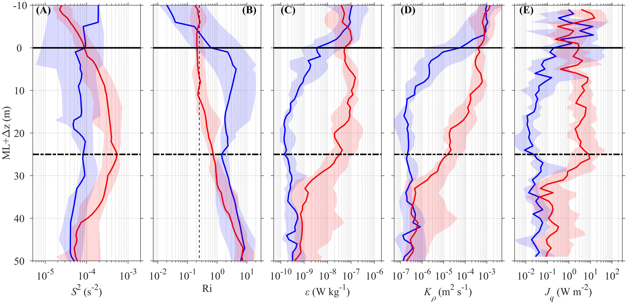
Figure 5 Vertical profiles of observed (A) shear variance (S²), (B) Richardson number (Ri; Ri = 0.25 is marked by the vertical dashed black line), (C) TKE dissipation rate (ε), (D) diapycnal diffusivity (K_ρ), and (E) turbulent heat flux (J_q) in the stations with (Stations 5–13, red) and without (Stations 1–4/14–16, blue) the presence of deep cycle turbulence. The solid curves are the ensemble median, and the shading area shows the 95% bootstrapped confidence interval. The vertical coordinate is of reference moving with the base of the mixed layer (ML). The thick solid and dash-dotted lines indicate the bases of the mixed layer and the deep cycle turbulence layer, respectively.

TABLE 1

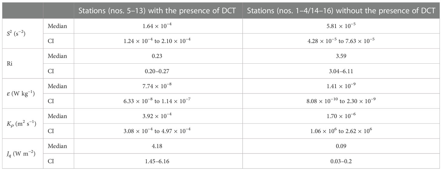
Table 1 Median values and 95% bootstrapped confidence intervals (CI) of shear variance (S²), Richardson number (Ri), TKE dissipation rate (ε), diapycnal diffusivity (K_ρ), and turbulent heat flux (J_q) over 0–10 m below the base of the mixed layer for the stations with and without the presence of deep cycle turbulence (DCT).

The discrepancies between our measurement and those in the eastern Pacific arise from different contributors to wind-related shear. In the eastern equatorial Pacific, the shear comes from the combined sources of zonal velocity differences within the Equatorial Undercurrent (EUC) and between the SEC and the EUC. Both sources are related to the easterly trade wind, which directly triggers the surface SEC and indirectly generates the eastward-shoaled EUC by establishing the zonal pressure gradient along the equatorial Pacific. In the WEP, our observed shear comes from the vertical difference of zonal velocity between the SEC and the WWE-induced eastward flow above. The EUC core in the western part is located at a depth of ~200 m, deeper than that in the eastern part. Thus, the shear within the EUC and at the interface layer between EUC and SEC contributes little to the DCT. When the WWE is absent, the shear in the deep cycle turbulence layer is not strong enough to produce a value of Ri close to 0.25, and the DCT vanishes. This explains why the DCT is not ubiquitous in the WEP.

The WWE-related DCT was also recently observed in the equatorial Indian Ocean (Pujiana et al., 2018). Their DCT occurred in the low Ri region also from the base of the mixed layer to the depth of the maximum S² with ε~O(10⁻⁷) W kg⁻¹. Their shear came from zonal velocity difference within the accelerating eastward Yoshida-Wyrtki jet, triggered by the WWE.

As is known to the authors, this is the first time that an episode of DCT has been observed in the WEP. The DCT may play an important role in the evolution of El Niño with the appearance of WWE and deserves future studies.

3.2 Interior mixing

The station-depth variations of N², S², Ri, ε, and K_ρ are shown in Figures 4C–G. In the interior ocean away from the mixed layer and deep cycle turbulence layer, the stratification and shear variance were strong over upper ~250 m with N²~O(10⁻⁴) s⁻² and S²~O(10⁻⁵) s⁻², and became weakened with depth in the layer of 250–750 m with N²~O(10⁻⁵) s⁻² and S²~O(10⁻⁶) s⁻² (Figures 4C, D). The values of S² are positively correlated with N², consistent with the nature of internal waves (MacKinnon and Gregg, 2003). The synchronous changes of N² and S² were combined to produce the equivalent Ri and ε from ~100 to 750 m (Figures 4C–F). The diapycnal mixing below 250 m was slightly evaluated due to the weakened stratification compared with that above 250 m (Figure 4G). Overall, the interior TKE dissipation rate and diapycnal diffusivity were very weak at the background levels with ε~O(10⁻¹⁰–10⁻⁹) W kg⁻¹ and K_ρ~O(10⁻⁷–10⁻⁶) m² s⁻¹, respectively. This is consistent with the fact that interior mixing induced by internal wave breaking is significantly reduced at low latitudes (Henyey et al., 1986; Gregg et al., 2003).

We next evaluate the performance of two parameterizations for turbulent dissipation in the ocean interior away from the mixed layer and the deep cycle turbulence layer in the WEP, namely, the MacKinnon–Gregg (MG) model and the Richardson number–based (Ri-based) model. To quantify the efficacy of different models, we define a measure of decade difference between the modeled (ε_model) and observed (ε_observation) values according to

$\begin{array}{ll}\sigma \text{ = [}\frac{1}{n}\sum _1^n{{\text{(log}}_{10}{\epsilon }_{model}{\text{-log}}_{10}{\epsilon }_{observation})}^2{]}^{\mathrm{1/2}},& (1)\end{array}$

where n is the number of data values (Wang et al., 2014).

On the basis of the idea that the turbulent dissipation rate associated with the spectral transfer of energy to smaller scales replies on simple ray-tracing equations, a succession of parameterizations, such as the MG and Gregg–Henyey–Polzin (GHP) models, is proposed (Henyey et al., 1986; Gregg, 1989; Polzin et al., 1995; MacKinnon and Gregg, 2003; MacKinnon and Gregg, 2005). Recently, the MG model has been demonstrated to have a better prediction skill than GHP model in the western Pacific (Liang et al., 2018; Liang et al., 2021). The MG model takes the form of ε_MG = ε₀(N/N₀)(S/S₀), where the reference values of N₀ and S₀ are both 3 cph. Figures 6A–C show the distributions of dissipation rates from observations and models as functions of bin-averaged stratification and shear variance. Scatter diagrams of observed versus modeled ε with straight lines depicting 1:10, 1:1, and 10:1 ratios are displayed in Figures 6D, E. First, we fit the MG model to observed ε through the least-square method and obtain ε₀ = 1.2 × 10⁻¹⁰ W kg⁻¹. The corresponding σ = 0.49 means an average difference of 0.49 decades between ε_MG and ε_observation(Figure 6D). The value of σ less than 1 suggests that the MG model can well reproduce observed ε within the same order of magnitude. This adds evidence to the fact that the interior turbulent dissipation is related to internal waves.

FIGURE 6

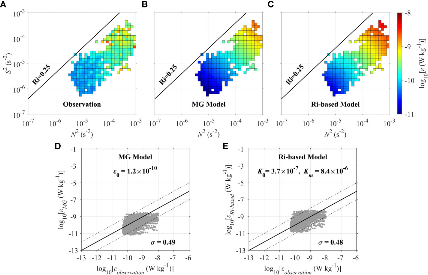
Figure 6 The distributions of (A) observed, (B) MG–modeled, and (C) Ri-based–modeled TKE dissipation rate with the mixed layer and deep cycle turbulence layer removed (ε, color shading) as functions of bin-averaged squared buoyancy frequency (N², x axis) and shear variance (S², y axis). Scatter diagrams of observed (ε_observation) versus (D) MG-modeled and (E) Ri-based–modeled TKE dissipation rates. The straight lines indicate the 1:1 (solid line), 1:10, and 10:1 (dashed lines) ratios.

The other parameterization examined here is the Ri-based model devised by Liu et al. (2017): K_ρ = K₀+K_m(1+Ri/0.25)⁻¹, where K₀ is a background minimum diffusivity corresponding to infinite Ri, and K_m is the maximum diffusivity corresponding to vanishing Ri. If we use K₀ = 2.1 × 10⁻⁶ m² s⁻¹ and K_m = 1.9 × 10⁻⁴ m² s⁻¹ obtained from Liu et al. (2017), then the value of ε is evidently overestimated by this parameterization with σ = 1.37 (figure not shown). On the basis of our observations, we can obtain K₀ = 3.7 × 10⁻⁷ m² s⁻¹ and K_m = 8.4 × 10⁻⁶ m² s⁻¹ through the non-linear least-squares regression. The modeled ε using the above new parameters well reproduces the observed ε within the same order of magnitude with σ = 0.48 (Figure 6E).

The above analysis suggests that the MG and Ri-based models both do a reasonably good job in scaling interior mixing in the WEP. However, the tuning parameters in both models vary in different regions, limiting the general applicability of the models. The underlying mechanisms for determining the tuning parameters need more observations to explore.

4 Summary and discussions

In this study, we report on microstructure measurements in the WEP and discuss the characteristics and influencing factors of equatorial diapycnal mixing. In the mixed layer, diapycnal mixing is mainly related to the wind forcing. With increasing westerly wind speed, the squared buoyancy frequency weakened and the shear instability with Ri < 0.25 occurred, resulting in the strong turbulence and diapycnal mixing with ε > O(10⁻⁸) W kg⁻¹ and K_ρ> O(10⁻⁴) m² s⁻¹, respectively, and the deepening mixed layer thickness from 20 m to 60 m. Most importantly, the WWE caused the eastward current in the surface and depressed the westward flowing SEC, resulting in strong shear and turbulence with ε~O(10⁻⁸–10⁻⁷) W kg⁻¹ at depths of 20–30 m below the base of the mixed layer. This strong turbulence resembles the DCT in the eastern equatorial Pacific in their occurring depth and their corresponding values of Ri and ε. Their difference is embodied in the different contributors to wind-related shear.

In the ocean interior away from the mixed layer and deep cycle turbulence layer, the diapycnal mixing is generally weak with the TKE dissipation rate ε∼O(10⁻¹⁰–10⁻⁹) W kg⁻¹ and diapycnal diffusivity K_ρ∼O(10⁻⁷–10⁻⁶) m² s⁻¹. This is consistent with the fact that interior mixing induced by internal wave breaking is significantly reduced at low latitudes. In terms of parameterization of the interior turbulence, the MG and Ri-based models both can do a good job with local fitting parameters.

The interior diapycnal diffusivity was very weak with K_ρ~O(10⁻⁷) m² s⁻¹, very close to the molecular diffusivity level. Under such conditions, the Osborn relationship with a constant mixing efficiency of 0.2 (Osborn, 1980) may fail to establish because isotropy is not satisfied (Shih et al., 2005). Bouffard and Boegman (2013, hereafter BB) proposed a modified model to calculate K_ρ depending on different buoyancy Reynolds (Re_b = ε/υN²) and Prandtl numbers (Pr = υ/κ_T, where υ is the kinematic viscosity and κ_T is the molecular thermal diffusivity). To compare the K_ρ obtained from the Osborn relationship and BB, we next applied the BB model as follows. The diapycnal diffusivity is calculated as K_ρ = 0.1υPr^−1/4Re_b^3/2 in the strongly stratified regime with 10^2/3Pr^−1/2 < Re_b< (3lnPr^1/2)², is set to the molecular level of ~1 × 10⁻⁷ m² s⁻¹ in the molecular regime with Re_b≤ 10^2/3Pr^−1/2, and is computed using the Osborn relationship in the residual regime with Re_b≥ (3lnPr^1/2)², respectively. Correspondingly, 56.3%, 31.4%, and 12.3% of our observed data fall into the above three regimes. Figures 4G, H show the time-depth variations of K_ρ obtained from the Osborn and BB model. Their orders of magnitudes are the same with a mean decadal difference of 0.24. Our study suggests that it is still feasible to use the Osborn relationship with a canonical mixing efficiency of 0.2 to calculate the interior diapycnal diffusivity, consistent with the results from Gregg et al. (2018).

Data availability statement

The datasets presented in this study can be found in online repositories. The names of the repository/repositories and accession number(s) can be found below: The VMP500 data, CTD data, LADCP data, and automatic weather station datasets access are available in Zenodo Research Shared data server (https://doi.org/10.5281/zenodo.7006854).

Author contributions

JW and FW initiated the idea and designed the observations. DS and JW analyzed the data and wrote the first draft of the paper. ZL and FW contributed to the interpretation of the results and the improvement of the manuscript.

Funding

The authors thank the reviewers for their comments. JW thanks the support from the National Natural Science Foundation of China (NFSC; grants 91958204 and 42222602), the Science and Technology Innovation Project of Laoshan Laboratory (LSKJ202203100), the Strategic Priority Research Program of the Chinese Academy of Sciences (grant XDA22000000), and TS Scholar Program. FW thanks the support from the NFSC (grants 41730534 and 42090040). ZL thanks the support from the NFSC (grant 91858201).

Conflict of interest

The authors declare that the research was conducted in the absence of any commercial or financial relationships that could be construed as a potential conflict of interest.

The reviewer CL declared a shared parent affiliation with the authors DS, JW and FW to the handling editor at the time of review.

Publisher’s note

All claims expressed in this article are solely those of the authors and do not necessarily represent those of their affiliated organizations, or those of the publisher, the editors and the reviewers. Any product that may be evaluated in this article, or claim that may be made by its manufacturer, is not guaranteed or endorsed by the publisher.

References

Bouffard D., Boegman L. (2013). A diapycnal diffusivity model for stratified environmental flows. Dynam. Atmos. Oceans 61–62, 14–34. doi: 10.1016/j.dynatmoce.2013.02.002

CrossRef Full Text | Google Scholar

Fine R. A., Lukas R., Bingham F. M., Warner M. J., Gammon R. H. (1994). The western equatorial pacific: A water mass crossroads. J. Geophys. Res. Oceans 99 (C12), 25063–25080. doi: 10.1029/94JC02277

CrossRef Full Text | Google Scholar

Gregg M. C. (1989). Scaling turbulent dissipation in the thermocline. J. Geophys. Res. Oceans 94 (C7), 9686–9698. doi: 10.1029/JC094iC07p09686

CrossRef Full Text | Google Scholar

Gregg M. C., D’Asaro E. A., Riley J. J., Kunze E. (2018). Mixing efficiency in the ocean. Annu. Rev. Mar. Sci. 10 (1), 443–473. doi: 10.1146/annurev-marine-121916-063643

CrossRef Full Text | Google Scholar

Gregg M. C., Peters H., Wesson J. C., Oakey N. S., Shay T. J. (1985). Intensive measurements of turbulence and shear in the equatorial undercurrent. Nature 318 (6042), 140–144. doi: 10.1038/318140a0

CrossRef Full Text | Google Scholar

Gregg M. C., Sanford T. B., Winkel D. P. (2003). Reduced mixing from the breaking of internal waves in equatorial waters. Nature 422, 513–515. doi: 10.1038/nature01507

PubMed Abstract | CrossRef Full Text | Google Scholar

Henyey F. S., Wright J., Flatté S. M. (1986). Energy and action flow through the internal wave field: An eikonal approach. J. Geophys. Res. Oceans 91 (C7), 8487–8495. doi: 10.1029/JC091iC07p08487

CrossRef Full Text | Google Scholar

Hibiya T., Nagasawa M., Niwa Y. (2007). Latitudinal dependence of diapycnal diffusivity in the thermocline observed using a micro- structure profiler. Geophys. Res. Lett. 34, L24602. doi: 10.1029/2007GL032323

CrossRef Full Text | Google Scholar

Kaneko I., Takatsuki Y., Kamiya H., Kawae S. (1998). Water property and current distributions along the WHP-P9 section (137°–142°) in the western north pacific. J. Geophys. Res. Oceans 103 (C6), 12959–12984. doi: 10.1029/97JC03761

CrossRef Full Text | Google Scholar

Liang C., Shang X., Qi Y., Chen G., Yu L. (2018). Assessment of fine-scale parameterizations at low latitudes of the north pacific. Sci. Rep. 8, 10281. doi: 10.1038/s41598-018-28554-z

PubMed Abstract | CrossRef Full Text | Google Scholar

Liang C., Shang X., Qi Y., Chen G., Yu L. (2019). Enhanced diapycnal mixing between water masses in the western equatorial pacific. J. Geophys. Res. Oceans 124 (11), 8102–8115. doi: 10.1029/2019JC015463

CrossRef Full Text | Google Scholar

Liang C., Shang X., Qi Y., Chen G., Yu L. (2021). A modified finescale parameterization for turbulent mixing in the western equatorial pacific. J. Phys. Oceanogr 51 (4), 1133–1143. doi: 10.1175/JPO-D-20-0205.1

CrossRef Full Text | Google Scholar

Liu C., Huo D., Liu Z., Wang X., Guan C., Qi J., et al. (2022). Turbulent mixing in the barrier layer of the equatorial pacific ocean. Geophys. Res. Lett. 49, e2021GL097690. doi: 10.1029/2021GL097690

CrossRef Full Text | Google Scholar

Liu Z., Lian Q., Zhang F., Wang L., Li M., Bai X., et al. (2017). Weak thermocline mixing in the north pacific low-latitude western boundary current system. Geophys. Res. Lett. 44 (20), 10530–10539. doi: 10.1002/2017GL075210

CrossRef Full Text | Google Scholar

Lombardo C. P., Gregg M. C. (1989). Similarity scaling of viscous and thermal dissipation in a convecting surface boundary layer. J. Geophys. Res. Oceans 94 (C5), 6273–6284. doi: 10.1029/JC094iC05p06273

CrossRef Full Text | Google Scholar

Lueck R. G. (2016) RSI Technical note 028 calculating the rate of dissipation of turbulent kinetic energy. Available at: http://rocklandscientific.com/support/knowledge-base/technical-notes/ (Accessed March 27, 2022).

Google Scholar

MacKinnon J. A., Gregg M. C. (2003). Mixing on the late-summer new England shelf–solibores, shear, and stratification. J. Phys. Oceanogr 33 (7), 1476–1492. doi: 10.1175/1520-0485(2003)033<1476:MOTLNE>2.0.CO;2

CrossRef Full Text | Google Scholar

MacKinnon J. A., Gregg M. C. (2005). Spring mixing: Turbulence and internal waves during restratification on the new England shelf. J. Phys. Oceanogr 35 (12), 2425–2443. doi: 10.1175/JPO2821.1

CrossRef Full Text | Google Scholar

Menkes C. E., Lengaigne M., Vialard J., Puy M., Marchesiello P., Cravatte S., et al. (2014). About the role of Westerly wind events in the possible development of an El niño in 2014. Geophys. Res. Lett. 41 (18), 6476–6483. doi: 10.1002/2014GL061186

CrossRef Full Text | Google Scholar

Moum J. N., Caldwell D. R. (1985). Local influences on shear-flow turbulence in the equatorial ocean. Science 230 (4723), 315–316. doi: 10.1126/science.230.4723.315

PubMed Abstract | CrossRef Full Text | Google Scholar

Moum J. N., Perlin A., Nash J. D., McPhaden M. J. (2013). Seasonal sea surface cooling in the equatorial pacific cold tongue controlled by ocean mixing. Nature 500 (7460), 64–67. doi: 10.1038/nature12363

PubMed Abstract | CrossRef Full Text | Google Scholar

Nasmyth P. W. (1970). Oceanic turbulence (Vancouver: University of British Columbia).

Google Scholar

Osborn T. R. (1980). Estimates of the local rate of vertical diffusion from dissipation measurements. J. Phys. Oceanogr 10 (1), 83–89. doi: 10.1175/1520-0485(1980)010<0083:eotlro>2.0.co;2

CrossRef Full Text | Google Scholar

Philander S. G. H., Pacanowski R. C. (1980). The generation of equatorial currents. J. Geophys. Res. Oceans 85 (NC2), 1123–1136. doi: 10.1029/JC085iC02p01123

CrossRef Full Text | Google Scholar

Polzin K. L., Toole J. M., Schmitt R. W. (1995). Finescale parameterizations of turbulent dissipation. J. Phys. Oceanogr 25 (3), 306–328. doi: 10.1175/1520-0485(1995)025<0306:FPOTD>2.0.CO;2

CrossRef Full Text | Google Scholar

Pujiana K., Moum J. N., Smyth W. D. (2018). The role of turbulence in redistributing upper-ocean heat, freshwater, and momentum in response to the MJO in the equatorial Indian ocean. J. Phys. Oceanogr 48 (1), 197–220. doi: 10.1175/JPO-D-17-0146.1

CrossRef Full Text | Google Scholar

Richards K. J., Kashino Y., Natarov A., Firing E. (2012). Mixing in the western equatorial pacific and its modulation by ENSO. Geophys. Res. Lett. 39, L02604. doi: 10.1029/2011GL050439

CrossRef Full Text | Google Scholar

Richards K. J., Natarov A., Firing E., Kashino Y., Soares S. M., Ishizu M., et al. (2015). Shear-generated turbulence in the equatorial pacific produced by small vertical scale flow features. J. Geophys. Res. Oceans 120 (5), 3777–3791. doi: 10.1002/2014JC010673

CrossRef Full Text | Google Scholar

Ruddick B., Anis A., Thompson K. (2000). Maximum likelihood spectral fitting: The batchelor spectrum. J. Atmos. Ocean. Technol. 17 (11), 1541–1555. doi: 10.1175/1520-0426(2000)017<1541:MLSFTB>2.0.CO;2

CrossRef Full Text | Google Scholar

Shay T. J., Gregg M. C. (1986). Convectively driven turbulent mixing in the upper ocean. J. Phys. Oceanogr 16 (11), 1777–1798. doi: 10.1175/1520-0485(1986)016<1777:CDTMIT>2.0.CO;2

CrossRef Full Text | Google Scholar

Shih L., Koseff J., Ivey G., Ferziger J. (2005). Parameterization of turbulent fluxes and scales using homogeneous sheared stably stratified turbulence simulations. J. Fluid Mech. 525, 193–214. doi: 10.1017/S0022112004002587

CrossRef Full Text | Google Scholar

Smyth W. D., Moum J. N. (2013). Marginal instability and deep cycle turbulence in the eastern equatorial pacific ocean. Geophys. Res. Lett. 40 (23), 6181–6185. doi: 10.1002/2013GL058403

CrossRef Full Text | Google Scholar

Thorpe S. A., Liu Z. (2009). Marginal instability? J. Phys. Oceanogr 39 (9), 2373–2381. doi: 10.1175/2009JPO4153.1

CrossRef Full Text | Google Scholar

Tsuchiya M., Lukas R., Fine R. A., Firing E., Lindstrom E. (1989). Source waters of the pacific equatorial undercurrent. Prog. Oceanogr 23 (2), 101–147. doi: 10.1016/0079-6611(89)90012-8

CrossRef Full Text | Google Scholar

Visbeck M. (2002). Deep velocity profiling using lowered acoustic Doppler current profilers: Bottom track and inverse solutions. J. Atmos. Ocean. Technol. 19 (5), 794–807. doi: 10.1175/1520-0426(2002)019<0794:DVPULA>2.0.CO;2

CrossRef Full Text | Google Scholar

Vladoiu A., Bouruet-Aubertot P., Cuypers Y., Ferron B., Schroeder K., Borghini M., et al. (2019). Mixing efficiency from microstructure measurements in the Sicily channel. Ocean Dyn 69, 787–807. doi: 10.1007/s10236-019-01274-2

CrossRef Full Text | Google Scholar

Wang J., Greenan B. J. W., Lu Y., Oakey N. S., Shaw W. J. (2014). Layered mixing on the new England shelf in summer. J. Geophys. Res. Oceans. 119, 5776–5796. doi: 10.1002/2014JC009947

CrossRef Full Text | Google Scholar

Warner S. J., Moum J. N. (2019). Feedback of mixing to ENSO phase change. Geophys. Res. Lett. 46 (23), 13920–13927. doi: 10.1029/2019GL085415

CrossRef Full Text | Google Scholar

Wolk F., Yamazaki H., Seuront L., Lueck R. G. (2002). A new free-fall profiler for measuring biophysical microstructure. J. Atmos. Ocean. Technol. 19 (5), 780–793. doi: 10.1175/1520-0426(2002)019<0780:ANFFPF>2.0.CO;2

CrossRef Full Text | Google Scholar

Zhang Z., Liu Z., Richards K., Shang G., Zhao W., Tian J., et al. (2019). Elevated diapycnal mixing by a subthermocline eddy in the western equatorial pacific. Geophys. Res. Lett. 46 (5), 2628–2636. doi: 10.1029/2018GL081512

CrossRef Full Text | Google Scholar

Zhang Z., Qiu B., Tian J., Zhao W., Huang X. (2018). Latitude-dependent finescale turbulent shear generations in the pacific tropical-extratropical upper ocean. Nat. Commun. 9, 4086. doi: 10.1038/s41467-018-06260-8

PubMed Abstract | CrossRef Full Text | Google Scholar