A Study on the Influence of Sand Median Grain Size on the Short-Term Recovery Process of Shorelines

Recently, the impacts of short-term erosion caused by storm waves on coastal damages are increasingly recognized as social issues, compared to those of long-term erosion from climate change or coastal development. The erosion caused by the storm wave has an episodic characteristic that the shoreline recovers gradually after retreating for a short-term. Furthermore, if shoreline changes caused by longshore sediment transport are not taken into consideration, the shoreline position is determined by following two physical parameters based on the bulk response model. The beach response factor determines converging ultimate erosion on the assumption that incident waves constantly affects a beach, which can be estimated according to the concept of Dean’s profile. On the contrary, the beach recovery factor affects the velocity of the shoreline retreat and recovery. Therefore, the parameter plays an important role to predict the peak erosion due to the storms. However, there are still insufficient researches to utilize it as an engineering design for erosion reduction. In this study, the two methodologies (i.e., approximation formula and statistical analysis) that estimates peak erosion width caused by the storms are compared to extract the beach recovery factor. During the process, it is confirmed that peak wave height has little impact on the beach recovery factor. Instead, it is mainly determined by the median grain size. Also, the beach recovery factor is estimated as a function of median grain size based on the shoreline and sand survey data conducted over ten years. Among the 41 surveyed sites along the east coast, 11 sites of straight-type shorelines that directly react to the incident waves were applied to consider only the short-term recovery process. To prove validity, the estimated applied into the real sea and then the results were compared to the shoreline data extracted from CCTV images. Using these results, the peak erosion width for a target wave event can be predicted with only median grain size. These study results are expected to be used as a concrete and practical means to manage the coast, in preparation for the current and future shoreline erosion threats.

1 Introduction

A beach is formed by accumulating sediments such as sand or gravel in an environment where waves are continuously incoming, and erosion and deposition are constantly repeated due to natural phenomena (typhoon, swell, sea-level rise, etc.) caused by disturbance of seawater. Among the numerous factors that induce beach erosion, the behavior of sediments due to wave dissipation is the most direct factor. Therefore, for the phenomenon of receding and advancing shorelines due to the incidence of storm waves, changes in the beach profile due to cross-shore sediment movement should be identified first.

The equilibrium beach profile is formed by balancing the shoreward and seaward movements of cross-shore sediment transport, and Bruun (1954) empirically suggested a correlation with the median particle size of sand. After that, Dean (1977) applied constant wave energy dissipation in a unit volume, and theoretically derived the relational expression presented by Bruun (1954). In various fields such as beach nourishment (Dean, 1991), beach management (Park et al., 2019), and sea-level rise (Bruun, 1962; Dubois, 1990), it has become a means to obtain various engineering solutions to predict and solve catastrophic problems caused by coastal erosion. Recently, Kim et al. (2021) expressed the vulnerability of ultimate erosion in terms of sand grain size by applying the equilibrium beach profile equation of Dean (1977). In addition, the empirical formula derived in this way was compared with the correlation between wave energy and shoreline obtained by Yates et al. (2009) for 5 years of field observation, and the validity of its application was verified.

For optimal design of coastal engineering works for erosion reduction, it is desirable to physically analyze changes in the beach profile such as prediction of peak erosion width from sand particle size data, which is the most representative sediment movement factor. Partheniades (1965) firstly introduced an erodibility coefficient closely related to the grain size of sand to estimate the load of suspended sand according to shear stress. And the value was applied as the main physical coefficient of numerical modeling for the topographic change of the seabed, such as the settling velocity of sand. (Hanson, 1990; Hanson and Cook, 1997; Pritchard and Hogg, 2003; van Ledden et al., 2004; Stanev et al., 2007; Mathew and Winterwerp, 2017). Hydrodynamic processes (i.e., waves), erosion processes (i.e., critical shear stress and erodibility coefficient and so on), and deposition processes (i.e., settling velocity, concentration and beach recovery factor) are significant factors in interpreting changes in the beach profile (Krone, 1962; Partheniades, 1965). At the center of this series of physical processes, the seabed sand plays an important role in the physical process (Aberle et al., 2004; Ha and Maa, 2009; Jacobs et al., 2011; Forsberg et al., 2018). Nevertheless, these studies are limited to changes in the seabed. Therefore, as the utilization of shoreline position change has not yet materialized enough, clear and detailed research results are needed.

Beach recovery after storm wave incidence takes over months to years (Morton et al., 1994; Houser and Hamilton, 2009). Interpretation of the process of beach recovery is a research theme that is as essential as the process of erosion. Numerous bulk response models have been developed to investigate a shoreline retreat and recovery (Wright et al., 1985; Miller and Dean, 2004; Yates et al., 2009; Kim et al., 2021). Bulk response models introduce functions or coefficients that affect shoreline retreat and recovery. Among them, the coefficient included in the empirically derived model by Miller and Dean (2004) directly affects the shoreline response. And to derive a shoreline response model, Lim et al. (2022) introduced the beach recovery factor, which plays a role similar to that of the Miller and Dean (2004)’s model. Ultimate erosion is determined by the coastal environments and the beach recovery factor affect how shoreline position responds to the convergence of peak erosion caused by storm impact. Therefore, estimating the beach recovery factor plays an important role in predicting the magnitude of the episodic erosion in coastal engineering.

To predict shoreline evolution, bulk response models introduced a coefficient or a function to work as the beach recovery factor in the past, rather than directly introducing the beach recovery factor. Wright et al. (1985) proposed the beach recovery factor as the relative size of the incoming wave due to wave imbalance. Although Miller and Dean (2004) analyzed how they are affected by the wave characteristics (i.e., wave height, period) and sand properties (i.e., sedimentation rate) in order to understand the physical feasibility of the beach recovery factor, there was a limitation in realizing it by applying it to the real field. Lesht (1989) reported that the beach recovery factor was proportional to the settling velocity, median grain size, and transport coefficient, and was inversely proportional to the closure depth by applying the cross-shore sediment transport equation proposed by Hanson and Larson (2000). Kim et al. (2021) verified the beach recovery factor correlates with the elapsed time from peak wave height to peak erosion by applying storm wave scenario to ODE (ordinary differential equation) model results. Recently, Lim et al. (2022) presented research results that clarified the specific physical meaning of the beach recovery factor by introducing the concept of the horizontal behavior of suspended sediment. However, despite numerous researches, there are yet difficulties in extracting the beach recovery factor that is a physical parameter to predict shoreline changes, and applying them into the real sea.

Recently, Kim et al. (2021) expressed the peak erosion width due to storm waves as a function of beach response and recovery factors by applying shoreline survey data and ODE model results. In addition, Kim et al. (2021) and Lim et al. (2021) verified that the shoreline survey data collected for many years follows a Gaussian distribution. Moreover, a method for statistically estimating the peak erosion width due to storm waves is proposed. In this study, a methodology to extract the beach recovery factor will be proposed by comparing two ways in which. Also, this paper studies how the beach recovery factor changes according to the wave and sand characteristics. The variability of the shoreline was analyzed from shoreline survey data obtained from the east coast of Korea for about 10 years, and this result was applied to reveal that the beach recovery factor can also be a function of the median grain size. Lastly, the applicability of this approach was verified by using CCTV monitoring data obtained from Maengbang Beach in East Sea. Figure 1 shows how the research was conducted to extract the beach recovery factor. If conditions are not given to carry out this, the result may be limited to the east coast of Korea, but it can be a means to estimate from the median grain size value easily.

FIGURE 1

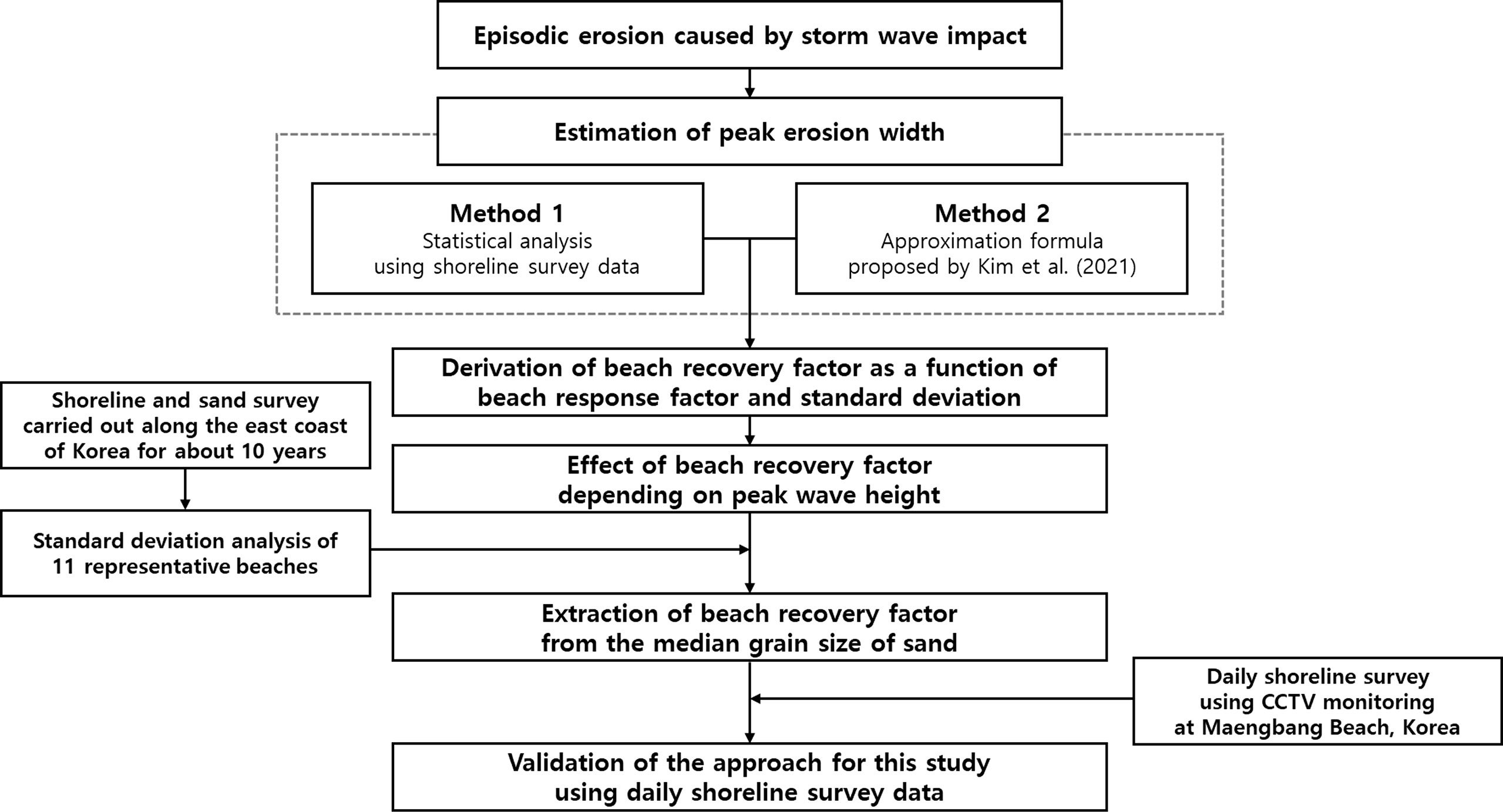
Figure 1 Process showing how the research is conducted to extract the beach recovery factor.

2 Estimation of Beach Recovery Factor

2.1 Beach Recovery Factor in Shoreline Response Model

Recently, Kim et al. (2021) proposed a bulk response model of the shoreline by the horizontal behavior of suspended sediment. The governing equation of their proposed model showed the type of ODE type similar to that of the shoreline response model proposed by Miller and Dean (2004). And a correlation of about 74% was obtained by substituting the predicted wave data as the input data of the model and comparing it with the shoreline fluctuation data obtained through CCTV analysis conducted by Montaño et al. (2020) at Tairua Beach, New Zealand (Lim et al., 2022). Recently, Lee et al. (2022) extended this model to a beach profile convergence model that can be simulated even in the macro-tidal environment and applied it to Tairua Beach to verify its applicability to real sea.

The shoreline response model (SLRM) governing the episodic changes in shoreline position due to storm wave incidence is given in Eq. (1) below.

$\begin{array}{ll}\frac{\mathbf{d}\mathbf{y}}{\mathbf{d}\mathbf{t}}={\mathbf{k}}_{\mathbf{r}}\left(\frac{{\mathbf{E}}_{\mathbf{b}}}{{\mathbf{a}}_{\mathbf{r}}}\mathbf{-}\mathbf{y}\right)& (1)\end{array}$

where y is the shoreline erosion width (positive value), k_r is a coefficient related to the recovery rate of the eroded shoreline as the beach recovery factor, and a_r is the beach response factor, which is a proportional constant between the wave energy at the breaking point and the equilibrium shoreline position as studied by Yates et al. (2009). And E_b is the wave energy at the breaking point defined by Yates et al. (2009) as

$\begin{array}{ll}{\mathbf{E}}_{\mathbf{b}}={{\mathbf{H}}_{\mathbf{s}\mathbf{,}\mathbf{b}}}^2/\mathbf{16}& (2)\end{array}$

Where H_s,b is the significant wave height at breaking point. And the unit of breaking wave energy E_b is m². If constant wave energy is incoming, the solution of the ODE model for Eq. (1) is as follows.

$\begin{array}{ll}\mathbf{y}=\frac{{\mathbf{E}}_{\mathbf{b}}}{{\mathbf{a}}_{\mathbf{r}}}\left[\mathbf{1}-\mathbf{e}\mathbf{x}\mathbf{p}\left(-{\mathbf{k}}_{\mathbf{r}}\mathbf{t}\right)\right]& (3)\end{array}$

After the equilibrium is reached and incident wave energy suddenly disappears, the shoreline position from that moment yields as follows.

$\begin{array}{ll}\mathbf{y}=\frac{{\mathbf{E}}_{\mathbf{b}}}{{\mathbf{a}}_{\mathbf{r}}}\mathbf{\text{exp}}\left(-{\mathbf{k}}_{\mathbf{r}}\mathbf{t}\right)& (4)\end{array}$

Based on the above equations, the beach recovery factor directly affects how the shoreline responds. On the other hand, the beach response factor a_r determines the ultimate shoreline position, which is subject to impacts on the incidence of constant wave energy. An approximate solution to obtain the beach response factor a_r can be obtained as follows (Kim and Lee, 2018).

$\begin{array}{ll}{\mathbf{a}}_{\mathbf{r}}\mathbf{\cong }\frac{\gamma {\mathbf{A}}^{3/2}}{\mathbf{16}}\left(\frac{{\tilde{\mathbf{H}}}_{\mathbf{b}}}{\sqrt{{\tilde{\mathbf{H}}}_b/\mathbf{\gamma }}\mathbf{-}\mathbf{f}}\right)& (5)\end{array}$

Here, A is a beach scale factor, y is a breaking index and ${\tilde{H}}_b$ is a representative breaking wave height. According to the study of Kim and Lee (2018), beach response factor a_r is almost the straight line in the high wave energy zone, not in the zone where incoming wave energy is low. Supplementary Figure 1 shows an equilibrium shoreline position caused by the wave energy and the beach response factor a_r can be estimated from the slope of the correlation curve. In addition, the slope of the curve is nearly constant in the high wave energy zone. This means that the beach response factor a_r is nearly constant in the storm wave range. Kim et al. (2021) applied a representative wave height ${\tilde{H}}_b$ of 6m to the storm wave. However, it is necessary to study whether the value is representative of storm waves in all regions. And a proportional constant f = 1.51 m^1/2 was proposed. Kim et al. (2021) obtained reasonable agreement by comparing the beach response factor a_r obtained from Eq. (5) with that obtained from the California field observation data of Yates et al. (2009).

Also, Eqs. (3)-(4) show that the beach recovery factor k_r directly affects time required to reach the equilibrium when the shoreline recovers or retreats. However, there seems to be no doubt that researches on the beach recovery factor k_r are lacking yet.

2.2 Peak Erosion Width

2.2.1 Formula for Peak Erosion Width by Elapsed Time

Kim et al. (2021) presented a method for easily determining the beach recovery factor k_r from the characteristics of the ODE expression of Eq (1). In Eq (1), dy/dt becomes 0 when the peak erosion width occurs based on the ODE type. Therefore, when the elapsed time from peak wave height to peak erosion is τ by applying the storm wave scenario function of Kim et al. (2021) as a storm wave event, the peak erosion width y_peak is expressed as below.

$\begin{array}{ll}{\mathbf{y}}_{peak}=\frac{E_b\left(\tau \right)}{a_r}& (6)\end{array}$

Kim et al. (2021) found the elapsed time τ as a function of only the beach recovery factor k_r independent of the beach response factor a_r through numerical analysis. Kim et al. (2021) expressed the following equation to calculate the peak erosion width y_peak as a function of the average annual wave,

$\overline{H}$ the incident wave conditions

$H_p^o$ and E_b, and the beach characteristic factors a_r and k_r.

$\begin{array}{ll}{\mathbf{y}}_{\mathbf{p}\mathbf{e}\mathbf{a}\mathbf{k}}={\mathbf{\alpha }}_{\mathbf{1}}{\left(\frac{{\mathbf{H}}_p^o}{\overline{\mathbf{H}}}\right)}^{{\mathbf{\alpha }}_2}\frac{{\mathbf{k}}_{\mathbf{r}}^{{\alpha }_3}{\mathbf{E}}_{\mathbf{b}}}{{\mathbf{a}}_r}& (7)\end{array}$

Here, the three coefficients a₁, a₂, and a₃ have values of 1.5, -0.275, and 0.911, respectively.

2.2.2 Statistical Analysis for Peak Erosion Width

Assuming that the probability distribution of shoreline variation follows a normal distribution, the relation of the return frequency F to the seasonal maximum variation

$y_F^s$ is given in terms of the standard deviation σ as follows.

$\begin{array}{ll}\mathbf{F}=\mathbf{1}-\frac{\mathbf{1}}{\mathbf{2}}\left[\mathbf{1}+\mathbf{e}\mathbf{r}\mathbf{f}\left(\frac{{\mathbf{y}}_{\mathbf{F}}^{\mathbf{s}}}{\mathbf{\sigma }\sqrt{2}}\right)\right]& (8)\end{array}$

However, since what we want to obtain corresponds to approximately the maximum fluctuation range $y_F^d$ for daily observed data, an additional conversion factor a given in terms of return frequency F is required.

$\begin{array}{ll}\mathbf{\alpha }\left(\mathbf{F}\right)={\left[\mathbf{60}\mathbf{F}+\mathbf{3.6}\right]}^{\mathbf{1}/\mathbf{4}}& (9)\end{array}$

Therefore, the following relation is applied to obtain the maximum variation $y_F^d$ for data observed daily from data observed once per season.

$\begin{array}{ll}{\mathbf{y}}_{\mathbf{F}}^{\mathbf{d}}\left(\mathbf{F}\right)=\alpha \left(\mathbf{F}\right){\mathbf{y}}_{\mathbf{F}}^{\mathbf{s}}\left(\mathbf{F},\mathbf{\sigma }\right)=\mathbf{\beta }\left(\mathbf{F}\right)\mathbf{\sigma }& (10)\end{array}$

where β is the total multiplication factor to the standard deviation and $y_F^s$ is obtained from Eq. (8) according to F and σ. Table 1 shows the factors that should be multiplied according to the return frequency using the standard deviation assuming that the shoreline observation data follows a normal distribution.

TABLE 1

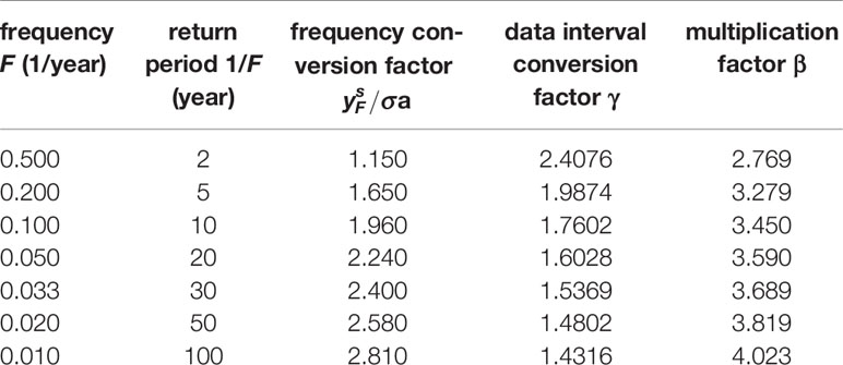
Table 1 Conversion rate and daily/seasonal variation extent according to return period.

Supplementary Figure 2 is the result of comparing shoreline evolution data extracted from CCTV almost every day from 1999 to 2017 at Tairua Beach, New Zealand to confirm the validity of this methodology (Montaño et al., 2020). By comparing it with the results of Eq. (10), almost similar results were obtained.

2.3 Estimation of Beach Recovery Factor

As described in Section 2.2, there are two methods for estimating the peak erosion width caused by storm waves. The approximate equation proposed by Kim et al. (2021) requires the extraction of beach characteristic factors a_r and k_r to obtain the peak erosion width. On the other hand, a sufficient number of shoreline survey data is required for statistical analysis to obtain the peak erosion width. Therefore, if the shoreline survey data have been accumulated enough for statistical analysis, the beach recovery factor can be estimated by comparing the two methods. If we equalize Eqs. (7) and (10), we get the following result for any return frequency F.

$\begin{array}{ll}{\mathbf{y}}_{\mathbf{p}\mathbf{e}\mathbf{a}\mathbf{k}}\left(\mathbf{F}\right)\mathbf{=}{\mathbf{\alpha }}_{\mathbf{1}}{\left(\frac{{\mathbf{H}}_{\mathbf{p},\mathbf{F}}^{\mathbf{o}}}{\overline{\mathbf{H}}}\right)}^{{\mathbf{\alpha }}_{\mathbf{2}}}\frac{{\mathbf{k}}_{\mathbf{r}}^{{\mathbf{\alpha }}_{\mathbf{3}}}{\mathbf{E}}_{\mathbf{b},\mathbf{F}}}{{\mathbf{a}}_{\mathbf{r}}}=\mathbf{\beta }\left(\mathbf{F}\right)\mathbf{\sigma }& (11)\end{array}$

If we arrange Eq. (11) for the beach recovery factor k_r we want to obtain, it is as follows.

$\begin{array}{ll}{\mathbf{k}}_{\mathbf{r}}^{{\mathbf{\alpha }}_{\mathbf{3}}}\mathbf{\cong }\frac{\mathbf{\beta }}{{\mathbf{\alpha }}_{\mathbf{1}}{\mathbf{E}}_{\mathbf{b},\mathbf{F}}}{\left(\frac{{\mathbf{H}}_{\mathbf{p},\mathbf{F}}^{\mathbf{o}}}{\overline{\mathbf{H}}}\right)}^{-{\alpha }_2}{\mathbf{a}}_{\mathbf{r}}\mathbf{\sigma }=\mathbf{\delta }{\mathbf{a}}_{\mathbf{r}}\mathbf{\sigma }& (12)\end{array}$

where, δ is the same as the following equation.

$\begin{array}{ll}\mathbf{\delta }=\frac{\mathbf{\beta }\left(\mathbf{F}\right)}{{\mathbf{\alpha }}_{\mathbf{1}}{\mathbf{E}}_{b,\mathbf{F}}}{\left(\frac{{\mathbf{H}}_{\mathbf{p},\mathbf{F}}^o}{\overline{\mathbf{H}}}\right)}^{-{\mathbf{\alpha }}_2}& (13)\end{array}$

Kim et al. (2021) analyzed the extreme value of wave height by using 40-year hindercasting data provided by National Oceanic and Atmospheric Administration (NOAA) with the application of the Gumbel method. Figure 2 shows how a coefficient δ changes depending on return frequency F and peak wave height $H_{p,F}^o$ as a function of F by applying the result of Kim et al. (2021) into Eq. (13). Since the standard deviation and the beach response factor a_r are expressed by the beach scale factor A, it is assumed that the coefficients have no effect on the frequency and the variation of k_r by frequency is shown in Figure 2. Therefore, when the frequency decreases or the incident wave height increases, the k_r value tends to increase somewhat. However, it can be concluded that it is possible to apply almost the same value.

FIGURE 2

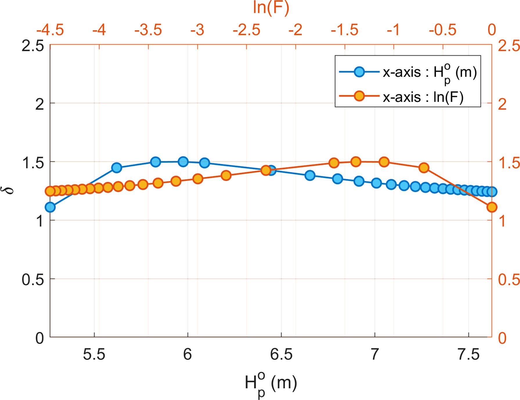
Figure 2 δ value according to the peak height of a storm wave event in the deep sea $H_{p,F}^o$ nd return frequency F.

3 Shoreline Variability at the Korean East Coast

In the east coast of Korea, littoral cells are classified based on relatively large-scale rivers, that are sources of incoming sediments, and the section judged to greatly restrict sediment movement in the direction of longshores, such as capes, was defined as the boundary of littoral cells. The littoral cells are classified into five shoreline types, such as straight, bow, beak, basket, and pocket-shaped, as shown in Supplementary Figure 3. Considering the inflow of rivers and longshore sediment transport, the total coastline of about 110 km from Myeongpa Beach in Goseong-gun (GW01) near the DMZ in Gangwon-do to Wolcheon Beach in Samcheok-si (GW41), the southern boundary of Gangwon-do is divided into 41 littoral cells. Most of the coast is made up of pure sandy beaches due to active littoral drift from the north. For each littoral cell, a reference line is set at an interval of about 300 m, and a total of 330 reference points are installed within the 41 field systems (The province of Gangwon, 2020).

Since 2010, shoreline surveys have been conducted four times a year in consideration of seasonal effects, and seafloor quality surveys to analyze the median particle size of sand through sampling have been conducted twice a year in winter and summer. Table 2 presents the basic information such as the shoreline type, number of survey data, average standard deviation of shoreline, and average representative particle diameter for each geologic system located in Figure 3 (The province of Gangwon, 2020). Except for 2 rocky shores (GW28 and GW37) and 1 unobservable section (GW35) of the 41 littoral cells, the shorelines of the remaining 38 littoral cells are classified into 13 straight, 12 bow, 8 beak, and 5 basket types.

TABLE 2

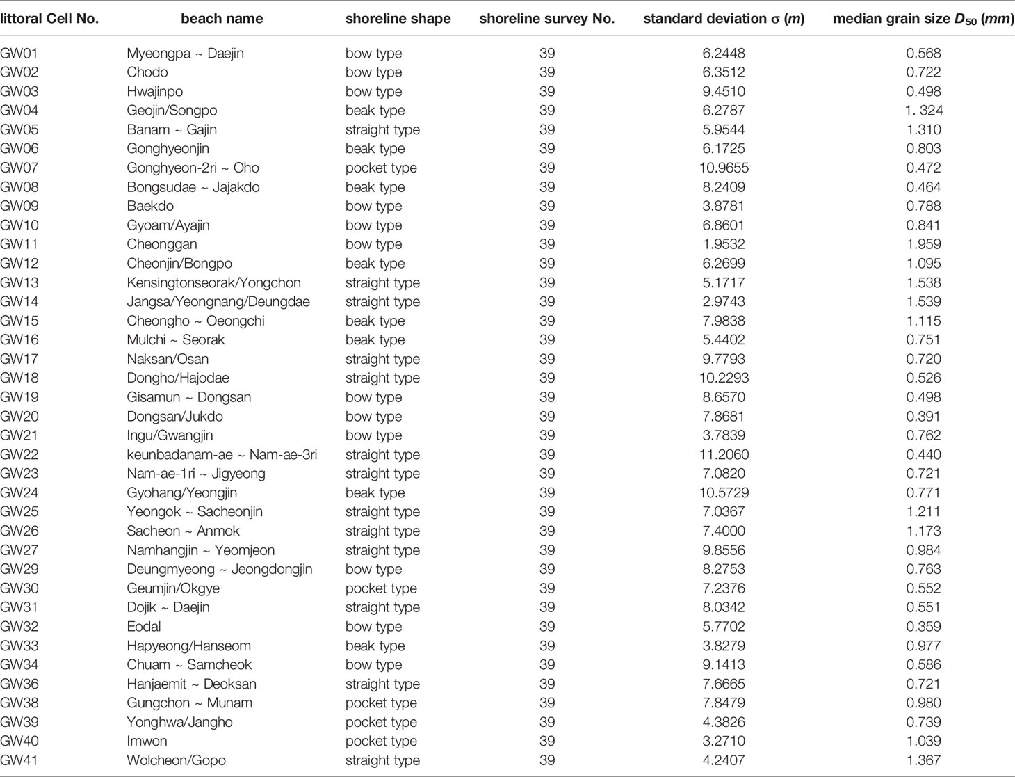
Table 2 Basic information of littoral cells in Gangwon-do (The province of Gangwon, 2020).

FIGURE 3

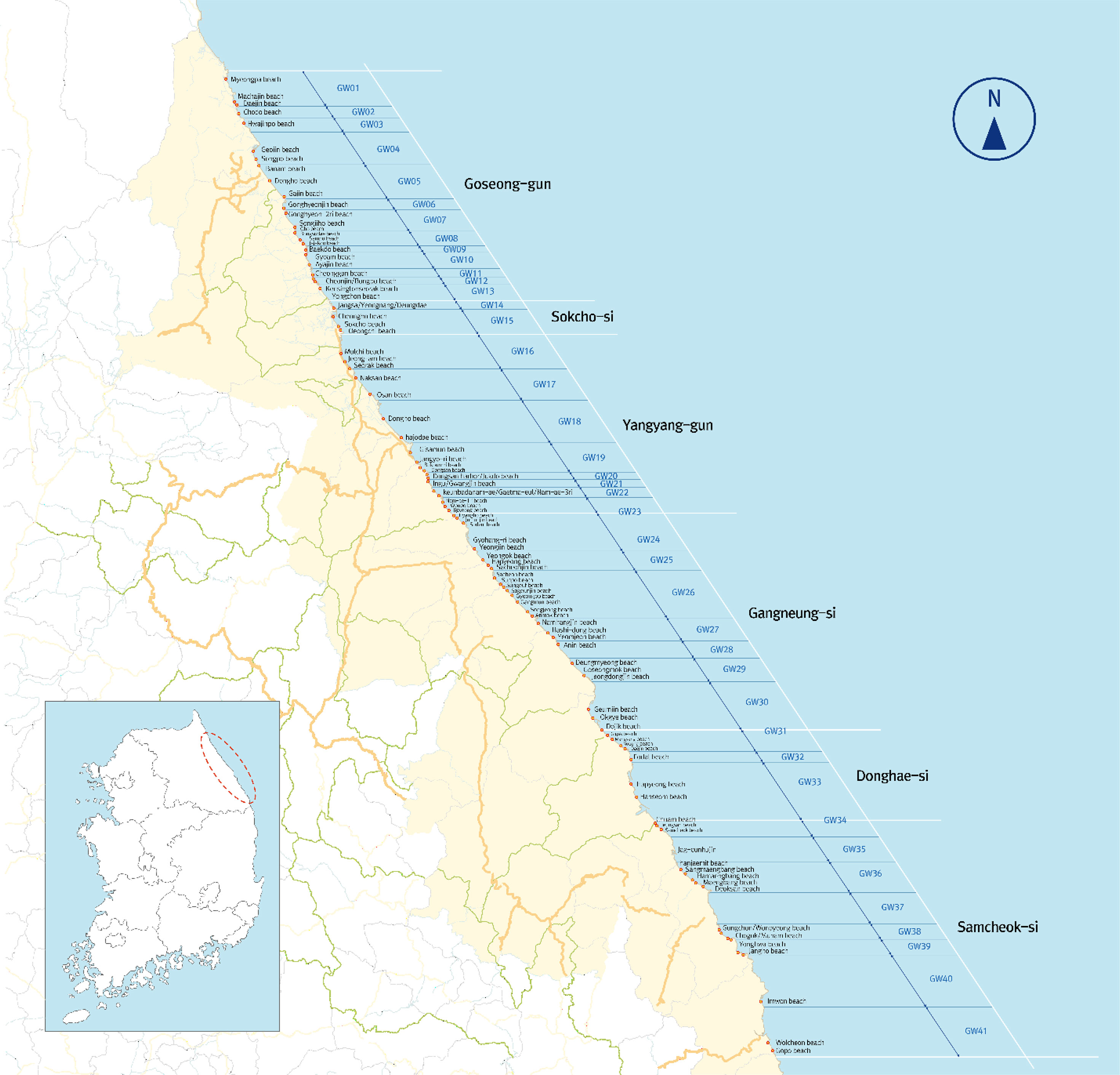
Figure 3 Location of littoral cells in Gangwon-do (The province of Gangwon, 2020).

In this study, littoral cells of straight shoreline-type with minimal wave deformation were used to increase the reliability in estimating the beach recovery factor k_r. Although the beaches included in the littoral cell of GW14 and GW41 are straight types, they were excluded from the analysis target due to severe shoreline deformation caused by indiscriminate construction of coastal structures. And in order to minimize the effect of longshore sediment transport, only median grain size data and shoreline survey data from the central region away from both ends of the littoral cell were applied. Table 3 shows the representative littoral cell information used in this study. And Figure 4 shows the probability distribution of shoreline change data surveyed on 11 representative beaches of the east coast. Most of the distributions follow a normal distribution. In Table 3, A is a factor related to D₅₀ in swash zone, which was obtained from the table presented by Dean (1977).

TABLE 3

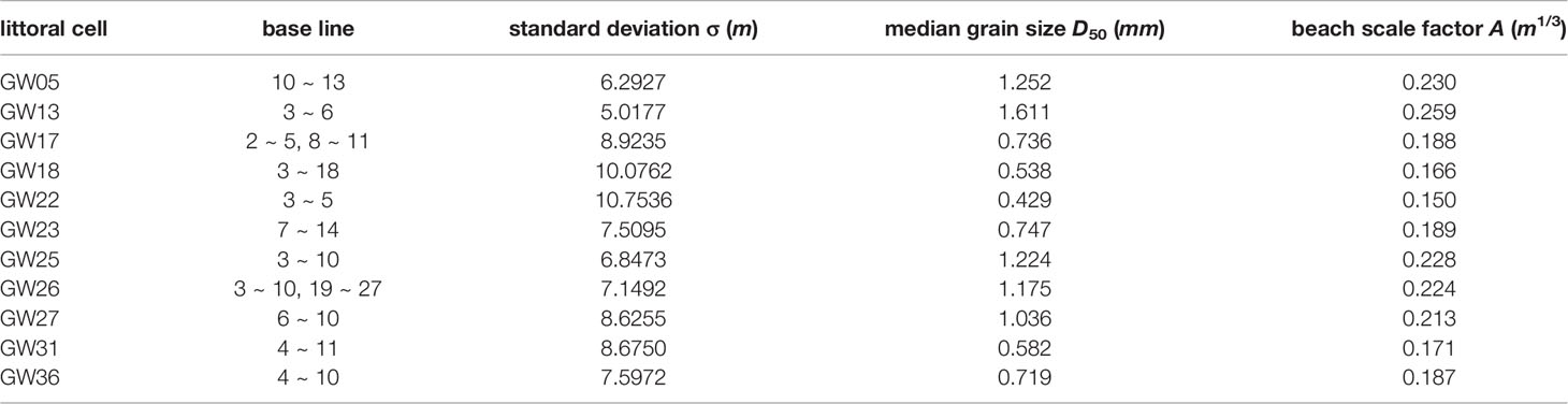
Table 3 Averaged standard deviation of shoreline change and averaged median grain size on the littoral cells of straight shoreline-type.

FIGURE 4

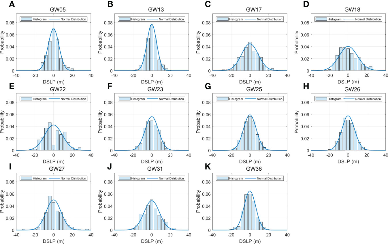
Figure 4 Probability distributions of shoreline data surveyed on 11 representative beaches of the east coast of Korea: (A) GW05 (B) GW13 (C) GW17 (D) GW18 (E) GW22 (F) GW23 (G) GW25 (H) GW26 (I) GW27 (J) GW31 (K) GW36.

4 Extraction of Beach Recovery Factor From Median Grain Size

Figure 5 shows the relationship between the median grain size D₅₀ and the shoreline standard deviation σ, which indicates shoreline variability, as presented in Table 3, and the standard deviation value tends to decrease as the median grain size increases. In other words, the larger the grain size of the sand, the smaller the erosion width. The standard deviation shows the correlation as shown in the following equations according to D₅₀ and A.

$\begin{array}{ll}\mathbf{\sigma }=\mathbf{-}\mathbf{4.04} {\mathbf{D}}_{\mathbf{50}}+\mathbf{11.64}& \text{(14a)}\end{array}$

$\begin{array}{ll}\mathbf{\sigma }=\mathbf{-}\mathbf{42.84} {\mathbf{A}}^{\mathbf{3}/\mathbf{2}}\mathbf{+}\mathbf{12.08}& \text{(14b)}\end{array}$

FIGURE 5

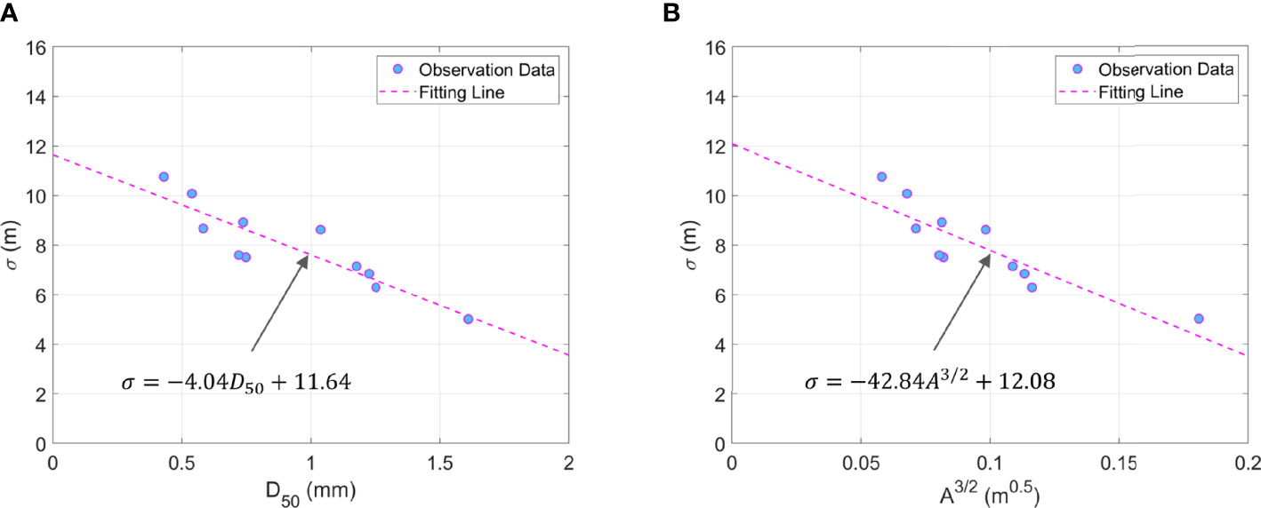
Figure 5 Correlation curve between grain size of sand and standard deviation: (A) median grain size D_50; (B) beach scale factor A.

For the median grain size D₅₀ (i.e., Eq. (14a)), the determination coefficient (R²) of observed results and trend line is 0.798 (adjusted R² = 0.776 ; p-value = 2.12 ×10^-6 ).And for the beach scale factor A (i.e., Eq. (14b)), the determination coefficient (R²) of those results is 0.794 (adjusted R² = 0.771 ; p-value = 2.34 ×10^-6). These results show that the sand grain size plays an important role in short-term shoreline changes.

Figure 6 shows the trends of median grain size D₅₀ and beach scale factor A with k_r/a_r. Since the sand on the east coast is mainly composed of quartz, the distribution of specific gravity was found to be in the range of 2.0 to 2.7. And the porosity was investigated to have 0.4.

FIGURE 6

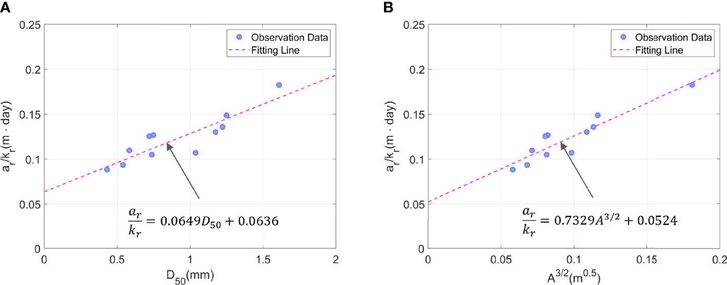
Figure 6 Correlation curve between grain size of sand and a_r/k_r: (A) median grain size D_50; (B) beach scale factor A..

Therefore, when D₅₀ is close to 0, it is expected to react without resisting even a small shear stress. Thus, although the erodibility is expected to increase considerably, it is expected to have yielding erodibility rather than infinity. Additionally, as D₅₀ is large, erodibility may tend to decrease continuously, so it is expected to show a high correlation with the exponential function or the inverse function. Figure 6 shows a correlation between sand characteristics and two factors (i.e., beach response and recovery factors) that have impacts on beach erosion. Figure 6A shows a yielding value of a_r/k_r from 0.0636 at A = 0 (unit: m·day) and tends to decrease as D₅₀ increases. Figure 6B shows a yielding value of a_r/k_r is 0.0524 at A = 0. It tends to decrease as A increases. However k_r/a_r that is the reciprocal of results obtained from Figure 6 is a function of D₅₀ and A as follows.

$\begin{array}{ll}\frac{{\mathbf{k}}_{\mathbf{r}}}{{\mathbf{a}}_{\mathbf{r}}}={\left(\mathbf{0.0649}{\mathbf{D}}_{\mathbf{50}}+\mathbf{0.0636}\right)}^{-\mathbf{1}}\mathbf{\cong }\frac{\mathbf{16}}{\left(\mathbf{1}+{\mathbf{D}}_{\mathbf{50}}\right)}& \text{(15a)}\end{array}$

$\begin{array}{ll}\frac{{\mathbf{k}}_{\mathbf{r}}}{{\mathbf{a}}_{\mathbf{r}}}={\left(\mathbf{0.7329}{\mathbf{A}}^{3/2}+\mathbf{0.0524}\right)}^{-1}\mathbf{\cong }\frac{\mathbf{20}}{\left(\mathbf{1}+\mathbf{14}{\mathbf{A}}^{3/2}\right)}& \text{(15b)}\end{array}$

For the median grain size D₅₀ (i.e., Eq. (15a)), the determination coefficient (R²) of observed results and trend line is 0.883 (adjusted R² = 0.854 ; p-value = 1.87 ×10^-6). And for the beach scale factor A (i.e., Eq. (15b)), the determination coefficient (R²) of those results is 0.980 (adjusted R² = 0.975 ; p-value = 1.87 ×10^-6 ).These results show that the sand grain size plays an important role in short-term shoreline changes. It is advantageous to estimate the beach recovery factor k_r using the beach scale factor A rather than the median grain size D₅₀.

In Eqs. (15a) and (15b), the beach response factor a_r can be obtained using Eq. (5). And by applying γ = 0.55, ${\tilde{H}}_b=6\hspace{0.17em}\text{m}$, and f = 1.51, which is usually applied to the representative significant waves, it has a value of $\frac{\gamma {\tilde{H}}_b}{\sqrt{{\tilde{H}}_b/\gamma }-f}=1.84$. Therefore, if the beach response factor a_r is expressed only as a function of the beach scale factor A, it is as follows.

$\begin{array}{ll}{\mathbf{a}}_r=\frac{{\mathbf{A}}^{3/2}}{\mathbf{16}}\left(\frac{\mathbf{\gamma }{\tilde{\mathbf{H}}}_{\mathbf{b}}}{\sqrt{{\tilde{\mathbf{H}}}_b/\mathbf{\gamma }}-\mathbf{f}}\right)=\mathbf{0.115}{\mathbf{A}}^{3/2}& (16)\end{array}$

Similarly, the beach recovery factor k_r is also approximately expressed as a function of only the beach scale factor A as follows.

$\begin{array}{ll}{\mathbf{k}}_{\mathbf{r}}=\frac{\mathbf{20}{\mathbf{a}}_{\mathbf{r}}}{\left(\mathbf{1}+\mathbf{14}{\mathbf{A}}^{3/2}\right)}=\frac{\mathbf{10}{\mathbf{A}}^{3/2}}{\mathbf{8}\left(\mathbf{1}+\mathbf{14}{\mathbf{A}}^{3/2}\right)}\left(\frac{\mathbf{\gamma }{\tilde{\mathbf{H}}}_{\mathbf{b}}}{\sqrt{{\tilde{\mathbf{H}}}_{\mathbf{b}}/\mathbf{\gamma }}\mathbf{-}\mathbf{f}}\right)=\frac{\mathbf{2.3}\mathbf{ }{\mathbf{A}}^{3/2}}{\left(\mathbf{1}\mathbf{+}\mathbf{14}{\mathbf{A}}^{3/2}\right)}& (17)\end{array}$

The beach response factor a_r and beach recovery factor k_r were obtained as a function of D₅₀ and A as given in Eq. (15). Therefore, sand grain size is the most dominant physical factor in estimating beach erosion and longshore sediment transport rate according to storm wave incidence. Table 4 shows the beach response factor a_r and beach recovery factor k_r were obtained according to D₅₀, assuming that the sand of the beach in Gangwon-do, Korea, flows from the watershed through the river, and the main component is quartz sand with a specific gravity of 2.65 and a porosity of 0.4. Using this, the beach recovery factor k_r and the beach response factor a_r can be obtained relatively easily using only the median grain size or beach scale factor. Lee et al. (2022) extracted the beach recovery factor from the median grain size using Eq. (17) and simulated not only the change of the shoreline position but also the change of the beach profile using the calculated value at Tairua Beach, New Zealand.

TABLE 4

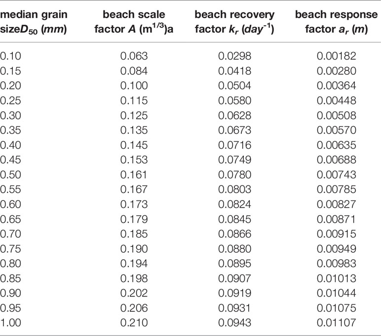
Table 4 k_r and a_r according to the median grain size of sand.

5 Discussion

In this study, beach response factor was estimated in terms of sand grain size by equating the statistical characteristics of the maximum erosion width by frequency obtained from long-term observation data with the formula of the peak erosion width obtained through numerical model experiments by applying the storm wave scenario function. In order to discuss the validity of this methodology, therefore, the temporal change of shoreline obtained by applying the beach recovery factor value given from the grain size of the sand at Maengbang Beach into ODE SLRM was compared with the shoreline evolution data using closed circuit television (CCTV).

The study site, Maengbang Beach, Samcheok-si, Gangwon-do, Republic of Korea is located in littoral cell GW 36 on the east coast (Figure 7). Maengbang Beach is a straight coast with a coastline of about 4.6 km in the northwest to southeast (NE-SE) direction, and has an average beach width of about 48 m (Figure 7).

FIGURE 7

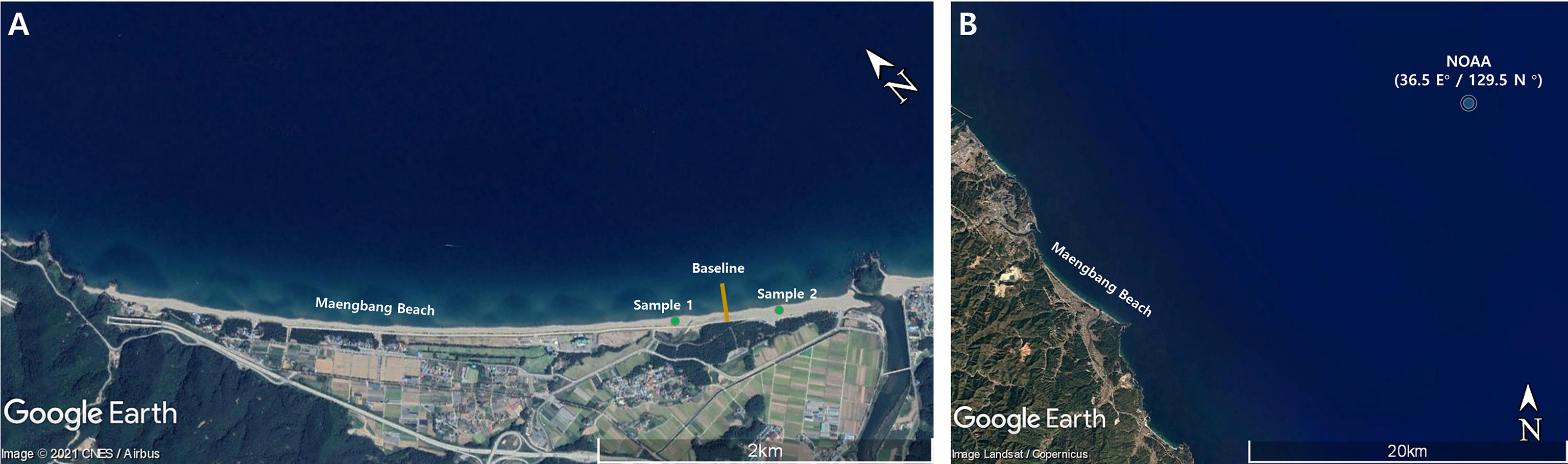
Figure 7 Location of Maengbang Beach: (A) sand and shoreline data (B) NOAA data (Google Earth Image).

Since 2010, the median grain size of sand at Maengbang Beach has been investigated twice a year (Table 5), and as a result, it is found that the median grain size is 0.69 mm. In addition, the standard deviation of the observed data is 0.14 mm, and it can be seen that the median particle size of the sand is at a 99% significance level from 0.33 mm to 1.05 mm. And it means that the beach recovery factor k_r has a value of 0.0862 day^-1 and the beach response factor a_r has a value of 0.00906 m (see Table 4). As the wave data for SLRM simulation, the NOAA wave data (37.5°N, 129.5°E; Figure 7B) located closest to Maengbang Beach was applied. Supplementary Figure 4 shows the wave height and wave energy at the breaking point, which is data at 3-hour intervals from August 22, 2015 to September 20, 2015.

TABLE 5

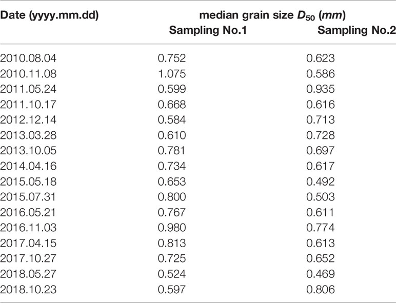
Table 5 Observation of median grain size at Maengbang Beach (The province of Gangwon, 2020).

Lim et al. (2022) recognized that the location of the shoreline extracted from CCTV images is affected by wave set-up and reflected this in the process of simulating SLRM to obtain numerical model results that are more similar to observations. In this study, the effect of wave set-up.

$\overline{\eta }$ was included in the numerical model results using the simple formula of Longuet-Higgins and Stewart (1964) as shown below.

$\begin{array}{ll}\overline{\mathbf{\eta }}=\frac{\mathbf{3}{\mathbf{\gamma }}^{\mathbf{2}}/\mathbf{8}}{\mathbf{1}\mathbf{+}\mathbf{3}{\mathbf{\gamma }}^{\mathbf{2}}/\mathbf{8}}{\mathbf{H}}_{\mathbf{b}}=\mathbf{\mu }{\mathbf{H}}_{\mathbf{b}}& (18)\end{array}$

where, μ becomes 0.1 for the breaking factor γ of 0.55. And the retreat of the wetting line on the CCTV image due to wave set-up was also approximated by applying the swash zone slope equation of Kim et al. (2014).

In addition, the average tidal level of Maengbang Beach is about 16.9 cm, and although the effect of the tide is not large, the effect of the tide is included in order to eliminate the discrepancy caused by the tide. The tide record measured at the Donghae Port tidal station (37°29’ N, 129°8’ E), which is located closest to Maengbang Beach, was used, and the data was provided by the Korea Hydrographic and Oceanographic Agency (KHOA). Supplementary Figure 5 shows the tide fluctuation at 1-hour interval for the duration for which comparison study is made. Since the SLRM in this paper did not reflect the effect of wave set-up and tides, the model was simulated by reflecting the change in sea levels caused by these effects.

To verify the validity of the methodology proposed in this study, the shoreline evolution data of Maengbang Beach were extracted using CCTV. Shorelines were extracted from geo-rectified images following the method of Lippmann and Holman (1989). Figure 8 shows a geometrically corrected image of CCTV data on Maengbang Beach. To extract shoreline data from the CCTV, it is important to define the location of the shoreline. Thus, a great number of researches have been conducted to define it from the past (Lippmann and Holman, 1989; Plant and Holman, 1997; Boak and Turner (2005). For the paper, CCTV images were captured continuously for a certain period of time and then compounded. On the image, the swash zone is clearly seen in a white band shape, which makes it possible to extract the shoreline for the paper (Lippmann and Holman, 1989; Plant and Holman, 1997). In addition, if the data was taken on a day with high wave height, it was removed to minimize the effects of large swash excursion in extracting the shoreline from the image (Davidson and Turner, 2009).

FIGURE 8

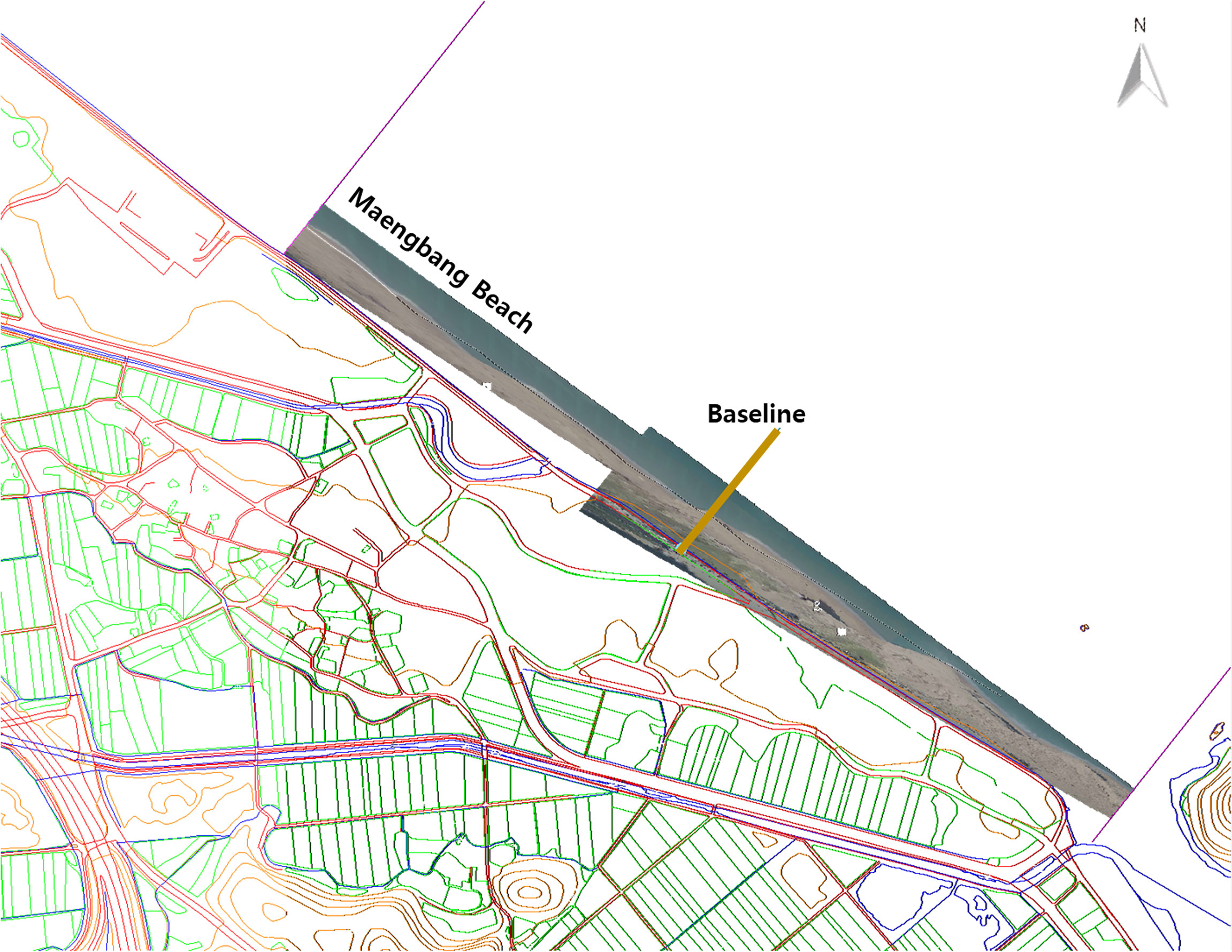
Figure 8 Geometry correction of CCTV images at Maengbang Beach.

Figure 9 is a figure comparing the SLRM results to which the beach recovery factor $k_r^o$ extracted by Eqs. (16)-(17) is applied with the CCTV Shoreline evolution data. For SLRM, the beach response factor $a_r^o$ of 0.00906 m and the beach recovery factor $k_r^o$ of 0.1293 day^-1 obtained for D₅₀ = 0.69 mm of Maengbang beach were applied. When these values ​​were applied, a correlation coefficient (Rxy) of 0.963 and a root mean square error (RMSE) of 1.484 m were obtained through consistency analysis with the observed values. In addition, in order to confirm that the beach recovery factor $k_r^o$ and the beach response factor $a_r^o$ have optimal values ​​in a certain range, each parameter was changed and consistency analysis was performed (Table 6). There is no problem using the factor of $k_r^o$ and $a_r^o$, but if there are factors that affect the shoreline change, such as the topographic environment, besides D₅₀, it is necessary to reflect the factors.

FIGURE 9

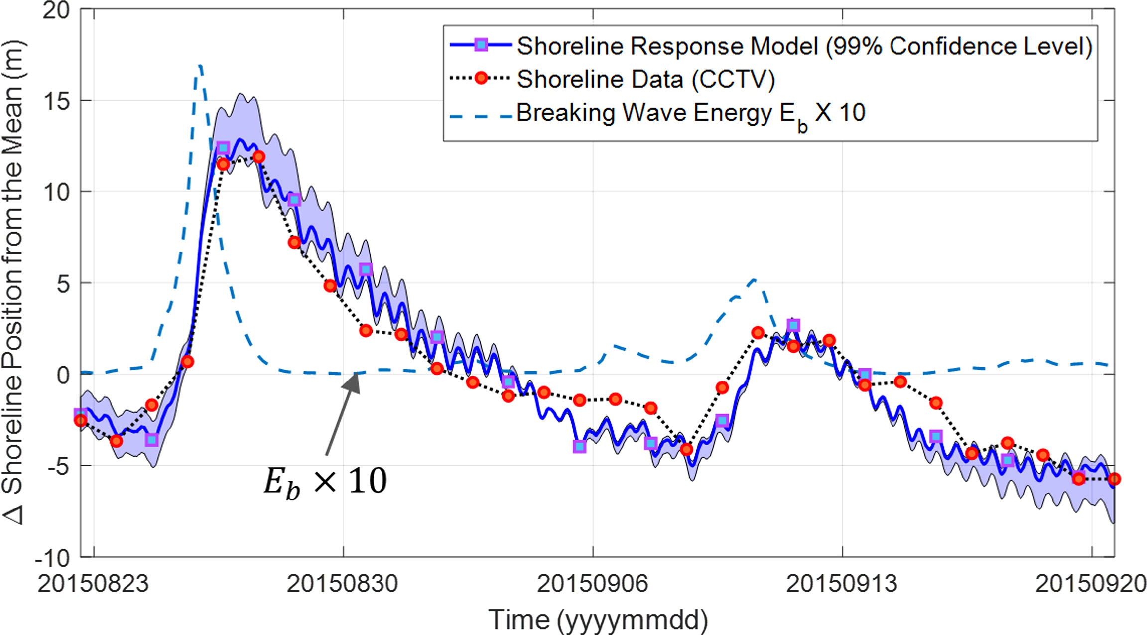
Figure 9 Comparison with shoreline data extracted from CCTV image and model results of SLRM applying the beach recovery and response factors of Eqs. (16)-(17).

TABLE 6

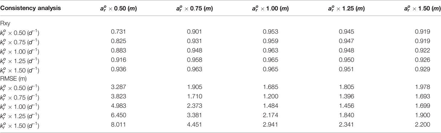
Table 6 Results of consistency index based on the response factor and recovery factor of Maengbang Beach.

6 Conclusion

The beach recovery factor is a representative physical coefficient that governs the short-term change of the shoreline position. This factor governs the characteristic of the sediment being separated from the beach profile due to the energy dissipation of the storm wave and then horizontally returning to the original beach position by the wave force of continuously incoming normal wave (Kim et al., 2021; Lim et al., 2022). In this study, an estimation formula for the beach recovery factor was presented as a function of the median grain size D₅₀ (or beach scale factor A) almost regardless of the incoming wave magnitude. The physical parameter was identified when ignoring the alongshore effect of sediment moving along the coast, such as longshore sediment transport.

As a methodology to present the beach recovery factor as a function of beach scale factor A, the maximum erosion width by return frequency statistically obtained from shoreline survey data was treated as the same as the formula for peak erosion width proposed by Kim et al. (2021). Shoreline survey was conducted over 10 years in Gangwon-do, Korea. Since the beach recovery factor obtained for each frequency is almost constant, it has little to do with the magnitude of the incoming wave energy and is considered to be a function of only the particle size of the sand. And by applying it to Maengbang Beach in Korea, a satisfactory simulation was obtained with an error of 1.484m as a result of applying the tidal and set-up effect into short-term shoreline change. The east coast of Korea is an environment with little influence of tides, with a tidal range of only 0.3 m. Therefore, the beach recovery factor obtained in this way can be applied to coastal environments with reduced astronomical tidal ranges such as the east coast, but the results of this study on the response of high tidal beaches with large tidal influences may be limited.

By applying the beach recovery factor suggested as a function of the median grain size in this study, the peak erosion width of the target wave can be predicted quantitatively and relatively accurately. Therefore, it is expected to be utilized as a concrete and practical means for coastal management in preparation for the current state and future threats of coastal erosion. The shoreline model mentioned in this paper deals only with cross-shore sediment transport. However, if the influence of longshore sediment transport is reflected together, it is possible to extend the shoreline change model including episodic erosion. Thus, it is expected that it will play an important role in improving the reliability of the shoreline change model in such a case.

Data Availability Statement

This study’s wave data are available in the WAVEWATCH III® Hindcast and Reanalysis Archives at the National Weather Service, National Oceanic and Atmospheric Administration (https://polar.ncep.noaa.gov/waves/hindcasts; NOAA, 2022). Other data sets used in this work can be requested by email from the first author (art3440@naver.com)

Author Contributions

CL, conceptualization, acquisition of data, visualization, and writing – original draft and editing. T-KK, acquisition of data and visualization. J-BK, acquisition of data. J-LL, conceptualization, supervision, validation, and writing – editing and review. All authors contributed to the article and approved the submitted version.

Funding

This research was supported by Korea Institute of Marine Science & Technology Promotion(KIMST) funded by the Ministry of Oceans and Fisheries, Korea(20180404). This research was supported by the SungKyunKwan University and the BK21 FOUR(Graduate School Innovation) funded by the Ministry of Education(MOE, Korea) and National Research Foundation of Korea(NRF).

Conflict of Interest

Author J-BK was employed by GeoSystem Research Corporation.

The remaining authors declare that the research was conducted in the absence of any commercial or financial relationships that could be construed as a potential conflict of interest.

Publisher’s Note

All claims expressed in this article are solely those of the authors and do not necessarily represent those of their affiliated organizations, or those of the publisher, the editors and the reviewers. Any product that may be evaluated in this article, or claim that may be made by its manufacturer, is not guaranteed or endorsed by the publisher.

Supplementary Material

The Supplementary Material for this article can be found online at: https://www.frontiersin.org/articles/10.3389/fmars.2022.906209/full#supplementary-material

Supplementary Figure 1 | Estimation of beach response factor a_r using correlation curve between equilibrium shoreline position and breaking wave energy.

Supplementary Figure 2 | Validity of extreme analysis methodology applying shoreline evolution data at Tairua Beach, New Zealand.

Supplementary Figure 3 | Category of shoreline shape: (a) straight type; (b) bow type; (c) basket type; (d) beak type; (e) pocket type (Google Earth and Kakao Map Image).

Supplementary Figure 4 | Temporal series of NOAA wave data at breaking point: (A) wave height; (B) wave energy.

Supplementary Figure 5 | Temporal series of tide data.

References

Aberle J., Nikora V., Walters R. (2004). Effects of Bed Material Properties on Cohesive Sediment Erosion. Mar. Geol. 207 1–4, 83–93. doi: 10.1016/j.margeo.2004.03.012

CrossRef Full Text | Google Scholar

Boak E., Turner I. L. (2005). Shoreline Definition and Detection: A Review. J. Coast. Res. 21, 688–703. doi: 10.2112/03-0071.1

CrossRef Full Text | Google Scholar

Bruun P. (1954). Coastal Erosion and the Development of Beach Profiles. Beach Erosion Board Technical Memo, No. 44, US Army Engineer Waterways Experiment Station, Vicksburg. http://hdl.handle.net/11681/3426

Google Scholar

Bruun P. (1962). Sea-Level Rise as a Cause of Shore Erosion. J. Waterway. Harbor. Div. 88. 1, 117–132. doi: 10.1061/JWHEAU.0000252

CrossRef Full Text | Google Scholar

Davidson M. A., Turner I. L. (2009). A Behavioral Template Beach Profile Model for Predicting Seasonal to Interannual Shoreline Evolution. J. Geophys. Res. 114, F01020. doi: 10.1029/2007JF000888

CrossRef Full Text | Google Scholar

Dean R. G. (1991). Equilibrium Beach Profiles: Characteristics and Applications. J. Coast. Res. 7, 53–84.

Google Scholar

Dean R. G. (1977). “Equilibrium Beach Profiles: U.S. Atlantic and Gulf Coasts,” in Technical Report No. 12 (Newark, DE: Department of Civil Engineering. University of Delaware).

Google Scholar

Dubois R. N. (1990). Barrier-Beach Erosion and Rising Sea Level. Geology 1811, 1150–1152. doi: 10.1130/0091-7613(1990)018<1150:BBEARS>2.3.CO;2

CrossRef Full Text | Google Scholar

Forsberg P. L., Skinnebach K. H., Becker M., Ernstsen V. B., Kroon A., Andersen T. J. (2018). The Influence of Aggregation on Cohesive Sediment Erosion and Settling. Cont. Shelf. Res. 171, 52–62. doi: 10.1016/j.csr.2018.10.005

CrossRef Full Text | Google Scholar

Ha H. K., Maa J. P.-Y. (2009). Evaluation of Two Conflicting Paradigms for Cohesive Sediment Deposition. Mar. Geol. 265 3–4, 120–129. doi: 10.1016/j.margeo.2009.07.001

CrossRef Full Text | Google Scholar

Hanson G. J. (1990). Surface Erodibility of Earthern Channels at High Stresses. Part I - Open Channel Testing. Trans. Am. Soc. Agric. Engineer. 33, 0127–31. doi: 10.13031/2013.31305

CrossRef Full Text | Google Scholar

Hanson G. J., Cook K. R. (1997). “Development of Excess Shear Stress Parameters for Circular Jet Testing,” in Proceedings of American Society of Agricultural Engineers ASCE, August 10–14 (Minneapolis, USA).

Google Scholar

Hanson H., Larson M. (2000). Simulating Coastal Evolution Using a New Type of N-Line Model. Proceedings of the 27th International Conference on Coastal Engineering (ICCE), July 16-21 (Sydney, Australia). doi: 10.1061/40549(276)219

CrossRef Full Text | Google Scholar

Houser C., Hamilton S. (2009). Sensitivity of Post-Hurricane Beach and Dune Recovery to Event Frequency. Earth Surf. ProcesS. Landforms. 34 613-, 628. doi: 10.1002/esp.1730

CrossRef Full Text | Google Scholar

Jacobs W., Le Hir P., Van Kesteren W., Cann P. (2011). Erosion Threshold of Sand–Mud Mixtures. Cont. Shelf. Res. 3110, S14–S25. doi: 10.1016/j.csr.2010.05.012

CrossRef Full Text | Google Scholar

Kim H., Hall K., Jin J.-Y., Park G. S., Lee J. (2014). Empirical Estimation of Beach-Face Slope and its Use for Warning of Berm Erosion. J. Measure. Eng. 21, 29–42.

Google Scholar

Kim T. K., Lee J. L. (2018). Analysis of Shoreline Response Due to Wave Energy Incidence Using Equilibrium Beach Profile Concept. J. Ocean. Eng. Technol. 322, 116–122. doi: 10.26748/KSOE.2018.4.32.2.116

CrossRef Full Text | Google Scholar

Kim T.-K., Lim C., Lee J. L. (2021). Vulnerability Analysis of Episodic Beach Erosion by Applying Storm Wave Scenarios to a Shoreline Response Model. Front. Mar. Sci. 8. doi: 10.3389/fmars.2021.759067

PubMed Abstract | CrossRef Full Text | Google Scholar

Krone R. B. (1962). “Flume Studies of the Transport of Sediment in Estuarial Shoaling Processes,” in Final Report. Hydraulic Engineering and Sanitary Engineering Research Laboratory (Berkeley, Calif., USA: University of California).

Google Scholar

Lee S., Lim C., Lee J. L. (2022). Prediction of Long-Term Beach Profile Evolution Due to Episodic Wave Incidence Under Tidal Environment. Front. Mar. Sci. 9. doi: 10.3389/fmars.2022.831262

PubMed Abstract | CrossRef Full Text | Google Scholar

Lesht B. M. (1989). Nearshore Dynamics and Coastal Processes: Theory, Measurement, and Predictive Models. Kiyoshi Horikawa. J. Geol. 97, 650–51. doi: 10.1086/629346

CrossRef Full Text | Google Scholar

Lim C., Kim T. K., Lee J. L. (2022). A Model of Shoreline Evolution for Sandy, Wave-Dominated Beaches. Geomorphology. Submitted for review.

Google Scholar

Lim C., Kim T. K., Lee S., Yeon Y. J., Lee J. L. (2021). Assessment of Potential Beach Erosion Risk and Impact of Coastal Zone Development: A Case Study on Bongpo-Cheonjin Beach. Nat. Haz. Earth Syst. Sci. 21, 3827–3842. doi: 10.5194/nhess-21-3827-2021

CrossRef Full Text | Google Scholar

Lippmann T. C., Holman R. A. (1989). Quantification of Sand Bar Morphology: A Video Technique Based on Wave Dissipation. J. Geophys. Res. 94, 995–1011. doi: 10.1029/JC094iC01p00995

CrossRef Full Text | Google Scholar

Longuet-Higgins M. S., Stewart R. W. (1964). Radiation Stresses in Water Waves; a Physical Discussion, With Applications. Deep-Sea. Res. Oceanog. Abstract. 11, 529–62. doi: 10.1016/0011-7471(64)90001-4

CrossRef Full Text | Google Scholar

Mathew R., Winterwerp J. C. (2017). Surficial Sediment Erodibility From Time-Series Measurements of Suspended Sediment Concentrations: Development and Validation. Ocean. Dynam. 67, 691–712. doi: 10.1007/s10236-017-1055-2

CrossRef Full Text | Google Scholar

Miller J. K., Dean R. G. (2004). A Simple New Shoreline Change Model. Coast. Eng. 51, 531–56. doi: 10.1016/j.coastaleng.2004.05.006

CrossRef Full Text | Google Scholar

Montaño J., Coco G., Antolínez J. A. A., Beuzen T., Bryan K. R., Cagigal L., et al. (2020). Blind Testing of Shoreline Evolution Models. Sci. Rep. 10, 2137. doi: 10.1038/s41598-020-59018-y

PubMed Abstract | CrossRef Full Text | Google Scholar

Morton R. A., Paine J. G., Gibeaut J. C. (1994). Stages and Durations of Post-Storm Beach Recovery, Southeastern Texas Coast, USA. J. Coast. Res. 884-908, 884–908.

Google Scholar

Park S. M., Park S. H., Lee J. L., Kim T. K. (2019). Erosion Control Line (ECL) Establishment Using Coastal Erosion Width Prediction Model by High Wave Height. J. Ocean. Eng. Technol. 33 (6), 526–534. doi: 10.26748/KSOE.2019.110

CrossRef Full Text | Google Scholar

Partheniades E. (1965). Erosion and Deposition of Cohesive Soils. J. Hydraul. Div-ASCE. 911, 105–139. doi: 10.1061/JYCEAJ.0001165

CrossRef Full Text | Google Scholar

Plant N. G., Holman R. A. (1997). Intertidal Beach Profile Estimation Using Video Images. Mar. Geol. 1401-2, 1–24. doi: 10.1016/S0025-3227(97)00019-4

CrossRef Full Text | Google Scholar

Pritchard D., Hogg A. J. (2003). Cross-Shore Sediment Transport and the Equilibrium Morphology of Mudflats Under Tidal Currents. J. Geophys. Res. 418 (C10), 3313. doi: 10.1029/2002JC001570

CrossRef Full Text | Google Scholar

Stanev E. V., Brink-Spalink G., Wolff J.-O. (2007). Sediment Dynamics in Tidally Dominated Environments Controlled by Transport and Turbulence: A Case Study for the East Frisian Wadden Sea. J. Geophys. Res. 112, C04018. doi: 10.1029/2005JC003045

CrossRef Full Text | Google Scholar

The province of Gangwon. (2020) “Research on the Actual Conditions of Coastal Erosion,” in Report of the Province of Gangwon, Gangwon, South Korea.

Google Scholar

van Ledden M., Wang Z.-B., Winterwerp H., de Vriend H. (2004). Sand–mud Morphodynamics in a Short Tidal Basin. Ocean. Dynam. 54, 385–391. doi: 10.1007/s10236-003-0050-y

CrossRef Full Text | Google Scholar

Wright L. D., Short A. D., Green M. O. (1985). Short-Term Changes in the Morphodynamic States of Beaches and Surf Zones: An Empirical Predictive Model. Mar. Geol. 62, 339–64. doi: 10.1016/0025-3227(85)90123-9

CrossRef Full Text | Google Scholar

Yates M. L., Guza R. T., O’Reilly W. C. (2009). Equilibrium Shoreline Response: Observations and Modeling. J. Geophys. Res.: Oceans. 114, C09014. doi: 10.1029/2009JC005359

CrossRef Full Text | Google Scholar