 Li Wei
 Lei Guan
- 1Sanya Oceanographic Institution, Ocean University of China, Sanya, China
- 2College of Marine Technology, Faculty of Information Science and Engineering, Ocean University of China, Qingdao, China
- 3Laboratory for Regional Oceanography and Numerical Modeling, Qingdao National Laboratory for Marine Science and Technology, Qingdao, China
Due to the application demand, users have higher expectations for the accuracy and resolution of sea surface temperature (SST) products. Recent advances in deep learning show great advantages in exploiting massive ocean datasets, and provides opportunities for investigating regional SST predictions in an efficiency approach. However, for deep learning-based SST prediction to be adopted by users, the output must be accurate. This paper investigates the 7-day SST prediction over the China seas and their adjacent waters at a 0.05° spatial resolution. To improve the prediction’s accuracy, we designed a deep learning model combining the three-dimensional convolution and long short-term memory under multi-input multi-output strategy. The Operational SST and Sea Ice Analysis (OSTIA) SST anomaly was used as training data. To test the model prediction ability, we verified the predicted results with the Sub-seasonal to Seasonal (S2S) prediction data from 2015 to 2019. Validation of the predicted SSTs using the OSTIA test datasets show that the root-mean-square error increases from 0.27°C to 0.53°C during the 1- to 7-day lead time, with predictability decreases from southeast to northwest in the study area. Furthermore, the comparison of predicted SST and S2S data with Argo shows that our model is slightly more accurate, which can achieve -0.08°C bias, with a standard deviation of 0.35°C for a 1-day lead time and -0.07°C bias, with a standard deviation of 0.59°C for a 7-day lead time. The results indicate that the proposed deep learning model is accurate and can be applied in regional daily SST prediction.
1. Introduction
Spatially-complete maps of predicted sea surface temperatures (SSTs) are in increased demand, specifically maps with a higher accuracy and greater resolution, which have an ever-expanding array of applications (Aparna et al., 2018). As different water temperatures attract and concentrate different fish species, predicted SST maps can help offshore fishermen determine the inhabited regions of target fish (IOCCG, 2009). For mariculture, SST is an essential factor affecting shrimp, fish, and other animals' growth and survival, and predicted SST data can be used to determine suitable locations to transfer marine cages (Roxanne, 2016). In addition, multiple studies have indicated that anomalously warm water can cause coral bleaching and hurricanes (Liu et al., 2013; McTaggart-Cowan et al., 2015). Thus, SST prediction can support a range of adaptive and management activities for marine ecosystems and tourism.
As a "learning from data" approach, deep learning has the advantages of computational efficiency, accuracy, transferability, flexibility and ease of use in ocean remote sensing data (Boukabara et al., 2019; Li et al., 2020). Numerical model-based forecasting face many challenges, and deep learning provides new opportunities for SST prediction (Boukabara et al., 2019). In 1997 and 1998, Tang et al. investigated SST prediction of the Niño region using a multilayer perceptron (MLP) (Tangang et al., 1997; Tangang et al, 1998a; Tangang et al. 1998b). Most early research chose meteorological factors as predictors in the study area (Tang et al., 2000; Hsieh, 2001; Wu et al., 2006; Garcia-Gorriz and Garcia-Sanchez, 2007; Aguilar-Martinez and Hsieh, 2009). Regarding whether the original data are preprocessed, Tangang et al. (Tangang et al. 1998b) thought that the sea level pressure data were significantly compressed after the extended empirical orthogonal decomposition. The model size was small, and the prediction accuracy was slightly improved. Li et al. (Li et al., 1996) believed that the network model had a strong learning ability for the original data. After preprocessing, for example, transforming SST into SST index as a prediction factor may lose much helpful information and reduce the model's prediction ability.
Recent studies mainly used SST or SST anomaly (SSTA) time series as predictors (Mahongo and Deo, 2013; Patil et al., 2013; Patil et al, 2016; Patil and Deo, 2017; Aparna et al, 2018). Moreover, researchers paid more attention to SST prediction at the spatial scale. In this kind of study, the coordinates of the SST were fixed and usually divided on regular grids. Each grid contained a sequence of predictors. In this scenario, only the future SST of each grid needs to be predicted. One solution was constructing a model for each grid and combining the outputs to form a regional SST prediction field. Zhang Q. et al. (2017) research on Bohai SST prediction at a spatial resolution of 0.25° showed that the long short-term memory (LSTM) network had higher prediction accuracy than the MLP network. Based on their research, Yang et al. (2017) proposed adding convolutional layers to the prediction model, and research in the East China Sea showed that the root-mean-square error (RMSE) was 0.41°C with a 1-day lead time and 0.63°C with a 7-day lead time. The advantage of this approach is that the prediction model is well targeted, and the prediction accuracy for a particular grid may be higher. However, it is more suitable for site-specific or small area SST predictions. In the case of high-resolution SST predictions for larger areas, many models need to be trained, which is computationally intensive. Another way was to construct a generic prediction model for all grids. Xiao et al. (2019) used the convolutional LSTM model with a spatial resolution of 0.25° to predict SSTs in the East China Sea (27.5° - 33°N, 123.5° - 127.5°E), and the results showed that the RMSE was 0.85°C when the lead time was seven days. Zhang et al. (2020) used the gated recurrent unit neural network to capture the SST time regularity. This approach is efficient in training and prediction but also requires deep mining of the spatio-temporal relationships in the regional SST. Shao et al. (Shao et al., 2021) first put sea surface height anomaly and SST through multivariate empirical orthogonal function analysis to establish the spatial relationship between the discrete points. Then the principal components were used as model inputs. The results of this experiment showed that the model had high prediction accuracy in the South China Sea. However, the method did not predict SSTs at depths less than 200m.
In addition to pre-processing the SST series, the spatial features of the original data can be mined directly by convolutional networks. The construction of SST spatial relationships mainly depends on two-dimensional (2D) convolution (Xu et al., 2020; Yu et al., 2020; Patil and Iiyama, 2022). In processing time-series sequences, three-dimensional (3D) convolution not only extracts the spatial features of the data but also exploits its time-varying features. Qiao et al. proposed (2021) 3D CNN and LSTM with Attention Mechanism model to predict SST in the Bohai Sea and the South China Sea. The method used the Pearson correlation coefficients and XGboost model to extract seasonal, long-period features of the SST data, which were then used as input to the 3D CNN model with the raw SST data. Recent studies showed that 3D convolution neural network-based models can better capture the complex spatiotemporal dynamical process than 2D neural networks (Kamangir et al, 2022). Our previous studies focused on the monthly mean SST prediction in 1- to 12-month lead time. The prediction results showed that training the model with the SSTA sequence can significantly improve the prediction accuracy compared with directly using the SST sequence (Wei et al., 2019). Moreover, we adopted ensemble learning method and constructed a Fully Connected Long Short-Term Memory-based Ensemble model under an iterative multi-step strategy to improve the long-term SST prediction stability (Wei et al., 2020).
In multi-step predictions of SST, the most commonly used method is direct multi-step, followed by iterative multi-step, and a less used method is the multiple-input multiple-output (MIMO) strategy, although this method has proven to be most effective in other prediction fields (Taieb et al., 2012). The selection of training data sets is crucial in training processes. The training data set with higher accuracy, greater resolution and rich SST feature details can improve the application value of prediction data. Evaluation of multiple SST L4 products indicated that the quality of OSTIA SST data had high quality in both offshore and open oceans (Xie et al., 2008; Woo and Park, 2020). Previous research also lacked an assessment of the proposed deep learning models with in situ data.
This paper aims to use a deep learning model to predict the SST in the China Seas and their adjacent waters within a 1- to 7-day lead time at a spatial resolution of 0.05° to improve the SST prediction accuracy in complex seas. In contrast to the study of Qiao et al. (2021), we used the SST interannual mean (SSTM) of three decades as seasonal long-period data. Furthermore, considering the strong interaction between the target SST and the adjacent SST in daily prediction, this study used the SSTA time series as a predictor and constructed a three-dimensional convolutional LSTM (3DConv-LSTM) prediction model based on a MIMO strategy. The predicted SSTA and SSTM were summed to obtain the predicted SST in the study area from 2015 to 2019. To evaluate the feasibility of the model in practical applications, we compared the predicted output of the model with the Sub-seasonal to Seasonal (S2S) prediction data.
The study's main contributions can be summarized as follows: We proposed a 3DConv-LSTM model for predicting SST in the China Seas and adjacent waters; Furthermore, compared with other deep learning-based SST prediction models, the model improved the accuracy of SST prediction in this sea area. The predictions were compared with in situ and numerical model data, showing that the model can be used for short-term predictions of regional SSTs.
2. Materials and methods
2.1. Data
2.1.1. OSTIA data
We used data produced by the Operational SST and Sea Ice Analysis (OSTIA) system developed by Met Office for model training and testing. The system is to meet the increasing demand for accurate high-resolution SST products by the ocean forecasting community, new coupled ocean-atmosphere system, and higher resolution numerical weather prediction systems (Donlon et al., 2012). We used two products generated under the OSTIA system. Their temporal coverage is 01/01/1985-12/31/2007 and 01/01/2007- present, respectively. Both products provide daily, 0.05° grid resolution, global coverage foundation SST data. Validation of the products demonstrates that they have a -0.1 K bias, with a standard deviation of 0.56 K and a -0.04 K bias, with a standard deviation of 0.34 K, respectively, compared to independent Argo in situ data in the global ocean (McLaren et al., 2014; McLaren et al., 2021). The OSTIA data can be downloaded at the Copernicus Marine Environment Monitoring Service (https://resources.marine.copernicus.eu/products).
2.1.2. Argo data
The Argo data is available at https://www.star.nesdis.noaa.gov/socd/sst/iquam/data.html. We selected the top value from each Argo temperature profile with a quality level of 5 falling within 3–5 m depth for consistency with the OSTIA product validation method (Roberts-Jones et al, 2012). Merchant and Corlett found that these Argo data provide a good estimate of foundation SST values after performing a three-way comparison between Argo, surface drifter, and AATSR data (Roberts-Jones et al., 2012).
2.1.3. S2S data
We used the numerical model data from the S2S database to compare the prediction results. The S2S database became available to researchers in May 2015. As S2S is a research-based project, it only provides near real-time forecasts with a delay of three weeks. At present, the database is updated regularly by 11 operational meteorological centers around the world. We selected the data provided by the European Centre for Medium-Range Weather Forecasts (ECMWF). The integrated forecasting system of the ECMWF consists of 51 ensemble members, with a bi-weekly forecast frequency. Due to the design of the forecast scheme, the final forecast is the bulk SST. This data can be obtained from China Meteorological Administration, which is one of the S2S database archiving center (http://s2s.cma.cn/), with a resolution is 1.5°×1.5° (Vitart et al., 2017).
2.2. Methods
In order to improve the accuracy of short-term prediction, we designed the 3DConv-LSTM model and used SSTA and SSTM sequences in the training and prediction process. The SSTM, as long-time seasonal period data, was eventually added to the predicted SSTA, which can improve the stability of the predictions. Furthermore, the SSTA data can enhance the model's representation of helpful information in training by removing significant seasonal signals. Considering the strong interaction between the target SST and the adjacent SST in daily prediction, this study used 3D convolution and pooling processes to extract the spatial and temporal characteristics around the target SSTA and established its temporal relationship using the LSTM. The following section introduces the prediction factors, the multi-step prediction strategy, and the model training and prediction processes in detail.
2.2.1. The predictor and strategies for multi-step prediction
For predicting the next stage of SST, we chose SSTA as the predictor variable. Using a subset from the OSTIA dataset, with a spatial range of 0–45°N, 105–135°E (601×901 grid), the data from January 1985 to December 2014 were used as the training set and the data from January 2015 to December 2019 as the test set. We first calculated the SSTM of three decades and then subtracted the SSTM from the SST to obtain the SSTA. Previous studies confirmed that using SSTA as a predictor can significantly improve prediction accuracy (Wei et al., 2019). Compared with the SST sequence, the SSTA sequence does not contain significant seasonal signals, which can improve the expression of meaningful information in the model.
This study used the MIMO strategy for multi-step SST prediction. Compared with the single output of direct and iterative strategies, this strategy is multi-output and considers the random dependence between output targets (Taieb et al., 2012). We also investigated the effects of iterative multi-step (IMS) and MIMO on 7-day prediction accuracy. As shown in Table 1, We performed 150 tests with different model parameters and calculated the average RMSE (, ,... ) for each step of the prediction. It can be found that the error accumulation occurs in the IMS strategy, while the MIMO strategy can maintain the stability of the prediction results. In training progress, the MIMO strategy learns the relationship f established between the predictors and the multiple-output data:
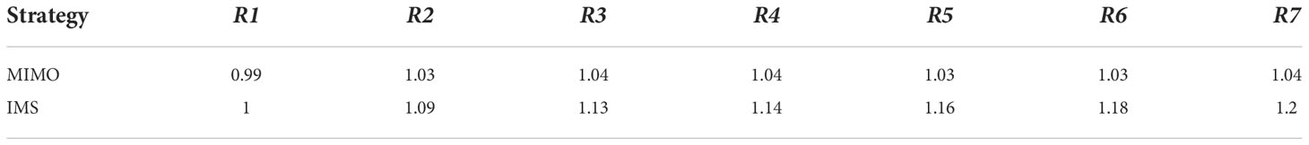
Table 1 The prediction performance of MIMO and IMS strategy for each step.
where T represents the length of the total space-time sequence for training, L is the length of the model output and is called a lead-time, d is the length of the model input, and W is the error term. In predicting progress, the trained model can be expressed as follows:
In this study, the SST is fixed and distributed on a regular grid. The total space-time sequence T for training is 10967, and the lead-time L is 7. The model input temporal length d is 21, which was set after the optimal hyperparameters search.
2.2.2. 3DConv-LSTM model
When applied to multi-step SST field prediction, it is desirable to capture the spatiotemporal information encoded in sequence fields. To this end, we proposed to use 3D convolutions to extract the spatiotemporal characteristics of the SSTA sequence and adopt LSTM to learn the relationship of spatiotemporal feature sequences with time. The short-term SST variability can be driven by ocean current systems. The Kuroshio in the region is a crucial component of the North Pacific subtropical circulation system. It includes the source of the Kuroshio, the Kuroshio in the East China Sea, the Kuroshio in the south of Japan and the Kuroshio Extension, which is the main current linking the western Pacific Ocean with the East China Sea, the South China Sea and the Japan Sea (Zhang C. et al., 2017). Considering the extensive impact of the Kuroshio on SSTs across the study area and the expensive computational cost of 3D convolutional-based models, we intended to construct a generic prediction model applicable to the entire region. Based on our previous work, we found that using the LSTM, rather than the fully connected layer, to learn the relationship can reduce the bias of the prediction results (Wei et al., 2019; Wei et al., 2020). The detailed descriptions on 3D convolutions and LSTM can reference the research of Ji et al. (Ji et al., 2012)and Hochreiter and Schmidhuber (Hochreiter and Schmidhuber, 1997).
The model’s hyperparameters were configured using a random search approach, and we first determined the maximum range for the spatial and temporal scale of the SSTA sequence, the maximum values of h, w and d in Figure 1. According to the study by Hosoda, which concluded that the meridional and temporal decorrelation scales of SST ranged from 1.5–3.0° and 1.2–2.0° (Hosoda and Kawamura, 2004), we set the maximum value of h and w to 55 grid points based on a spatial resolution of 0.05° for SST data. The setting maximum value of d is based on the suggestions of Zhang Q. et al. (2017) that the temporal input length is four times the model output length. Table 2 details the range of each hyperparameter in the random search. The search for hyperparameters focuses on selecting the optimal values of h, w and d from the setting range. To improve the random search efficiency, instead of using data from all spatial points (601*901), we selected data corresponding to 10,000 spatial points, uniformly distributed within the study area, to complete the search process. The search process was repeated 300 times. Each time, the model was trained under different parameter configurations and predicted SST values for 2014. Finally, we selected the parameter configuration with the best prediction accuracy based on the calculated RMSE, as shown in Table 3.
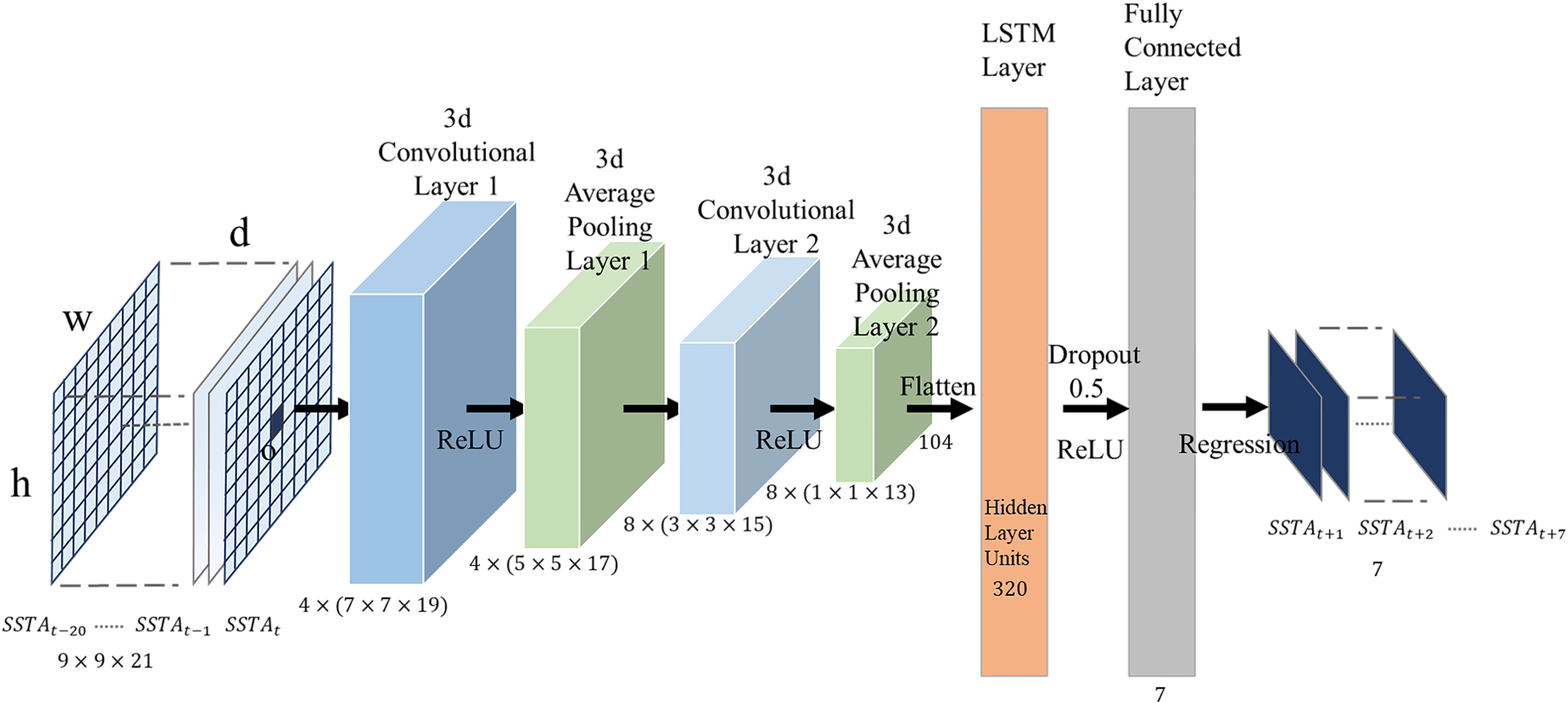
Figure 1 The 3DConv-LSTM structure.
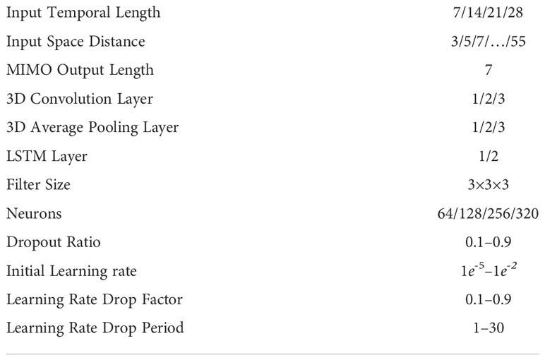
Table 2 The random research range of the hyperparameters.

Table 3 The selected configuration of the hyperparameters.
In the training process, the SSTA sequence with h, w and d of 9×9×21 undergoes 3D convolutional layers first, as shown in Figure 1. In this process, four convolution kernels with size of 3 × 3 × 3, multiply by the corresponding spatio-temporal data along the trajectory in a specific step, and then the product are summed to obtain the output value, and the final output feature map is also four 3D matrixes with size of 7×7×19. Then the feature maps undergo the average pooling layer. We set the number of convolution kernels in the third layer to 8. After the third layer of 3D convolution and the average pooling operation, we obtain eight 1×1×13 spatiotemporal features. Then, a mapping relationship is established through the fully connected LSTM with the SSTA sequence of 1–7 days at the target point o. The model uses the Adaptive moment estimation (Adam) optimization algorithm in the training process and selects RMSE as the loss function.
After the training is completed, in the prediction stage, the SSTA sequence output by the model is added to the corresponding SSTM to obtain the final SST prediction results. The deep learning model 3DConv-LSTM was developed using the MATLAB deep learning toolbox.
3. Results and discussions
The 3DConv-LSTM model made daily SST predictions in the China Sea and their adjacent waters from 2015 to 2019, with a lead time of 1 to 7 days. The prediction results were validated by comparison with the OSTIA SST, Argo in situ SST, and S2S data.
3.1. Comparison to OSTIA SST
Figure 2 shows the comparison of the predicted SSTs with the retained OSTIA SST timeseries from 2015 to 2019. The RMSE between the predicted SST and OSTIA is calculated within each 0.05° grid, which was used to assess the accuracy of the model. With a 1-day lead time, 99% of the daily RMSE are less than 0.4°C. The monthly RMSE is approximately 0.2–0.4°C, and the value in summer is slightly higher. A peak was observed in the daily RMSE on August 26th, 2015, which corresponds to a significant prediction difference in the Sea of Japan. The SST shows a mainly positive anomaly in the in the region from August 5th to 25th, which is the temporal input length of the model. However, the SST drops rapidly in one day on August 26th, with most areas exceeding -2°C. Because the large SST variations during a day, the prediction has a sever difference. In addition, SSTs in the region are also influenced by the strength of cold and warm currents in the north. Since the training dataset does not encompass that area, this may in part result in the differences observed in this area. A reduction in prediction accuracy can be seen as the lead time increases. The RMSE of the 5-year difference decreases from 0.27°C to 0.41°C with a 1- to 3-day lead time. A further slowly reduction from 0.41°C to 0.53°C occurs with a 3- to 7-day lead time. The impact of the lead time on prediction accuracy is evident with a 1- to 3-day lead time, but the predicted SST values still remain highly accurate. According to Hosoda et al.’s research, the temporal correlation of global SST is 1.5–3 days before and after (Hosoda and Kawamura, 2004). When the lead time is within the period of temporal correlation, the overall prediction accuracy is high and easily affected by the length of lead time. After exceeding the correlation period, the prediction accuracy decreases, and the impact of the lead time is not obvious.
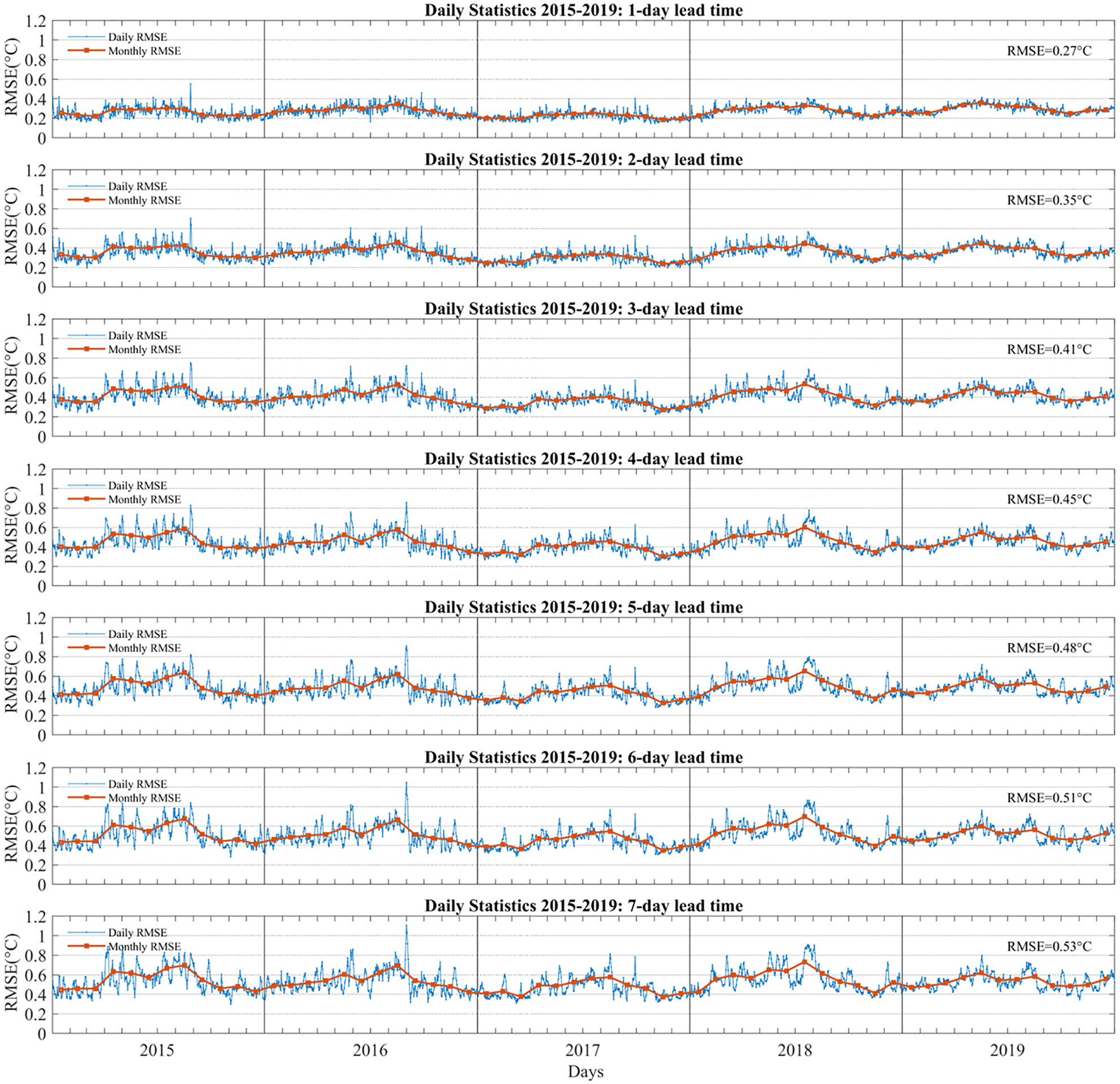
Figure 2 The daily RMSE (blue dots and line) and monthly RMSE (red dots and line) between predicted SSTs of the 3DConv-LSTM and OSTIA during 2015-2019 at a 1- to 7-day lead time.
The spatial pattern of the 5-year RMSE between the predicted SST and OSTIA was investigated. Figure 3 shows the RMSE distribution at different lead times. With a 1-day lead time, the RMSE near the Philippines are 0–0.2°C, and in the other areas they are mainly 0.2–0.4°C. The prediction accuracy in areas with high SST variability, such as the Yangtze River, the Yellow River Estuary, and coastal regions along the Korean Peninsula, are slightly lower, with RMSE between 0.4°C and 0.6°C. Using one model for the entire region may reduce prediction accuracy in sea areas with specific SST spatio-temporal characteristics. Overall, the predictability of SSTs gradually decreases from southeast to northwest with an increasing lead time.
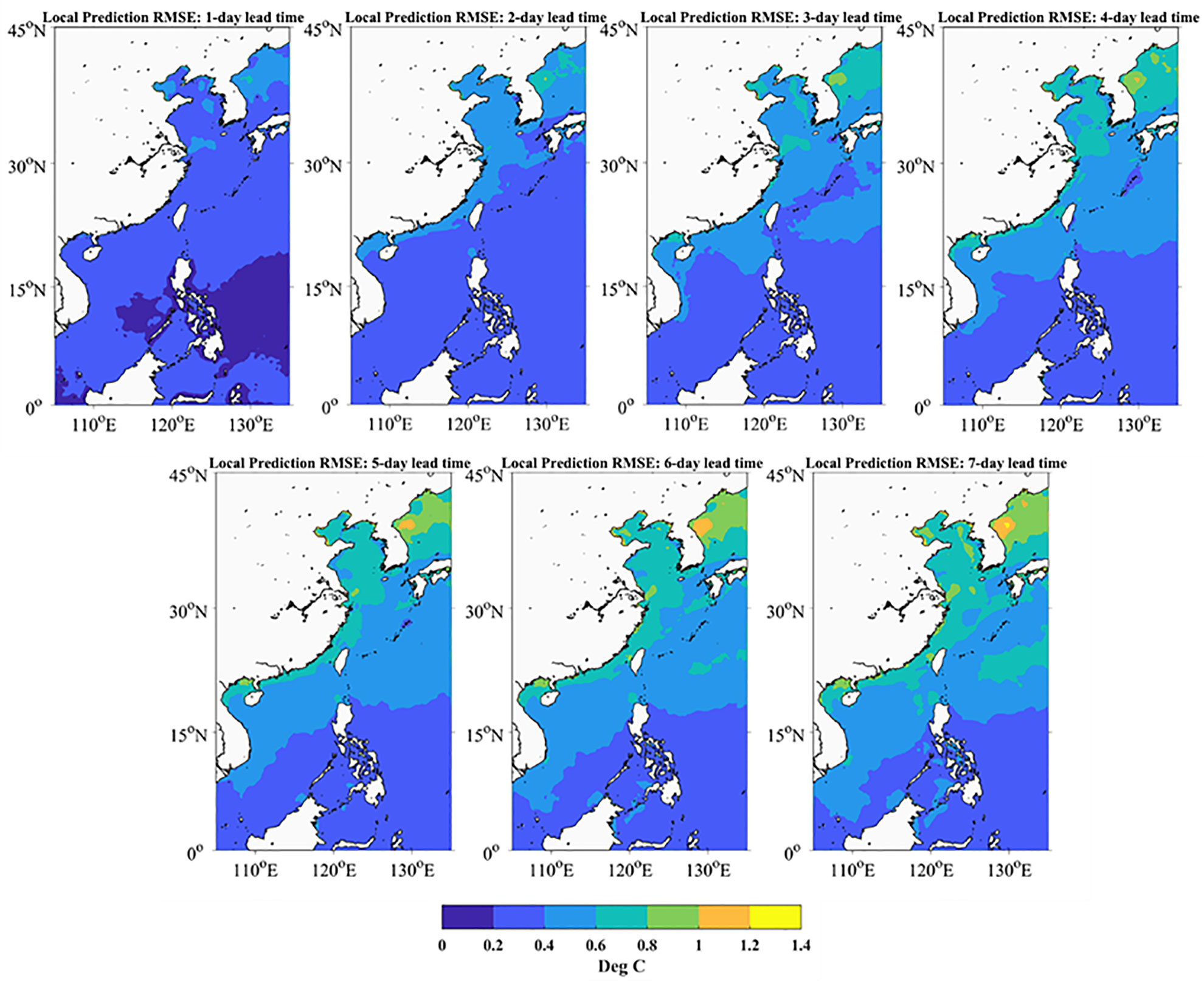
Figure 3 The spatial distribution of the RMSE between predicted SSTs of the 3DConv-LSTM and OSTIA during 2015-2019 at a 1- to 7-day lead time.
In the prediction stage, the model starts at a given date and steps forward by seven days in each step. Taking the model start date at December 31, 2018, and January 1, 2019, as an example, Figure 4 shows the spatial pattern of the SST difference between the prediction and the OSTIA SSTs. Panels (A) and (B) represent the model’s seven-day output at these two start times, respectively, from which the distribution of the SST difference changes with the prediction date. The difference does not continuously accumulate in the same area, and its spatial distribution patterns are similar in the first two prediction dates. Generally, the shorter the lead time is, the higher the prediction accuracy. The SST difference in most areas is within ± 1°C, and areas with significant differences usually appear in northeast of the study area. Overall, the spatial patterns of SST difference are related to the SST anomaly and lead time. At the same lead time, the SST differences are relatively large in the regions with high SST anomalies. The SST difference gradually increases with lead time, but the predicted SST is still consistent with the reserved OSTIA SST in 1- to 3-day lead time.
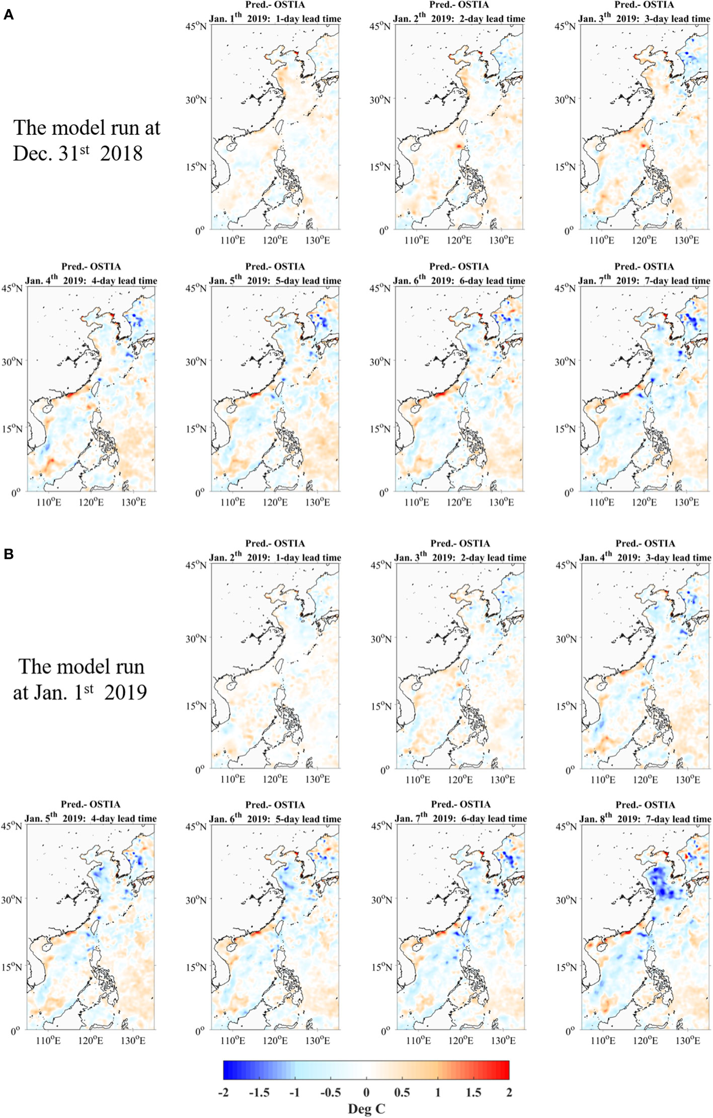
Figure 4 The spatial distribution of SST difference between predicted SSTs of the 3DConv-LSTM and OSTIA: (A) the 3DConv-LSTM start date at December 31, 2018; (B) the 3DConv-LSTM start date at January 1, 2019.
3.2. Comparison to other deep learning-based models
For the prediction accuracy of the 3DConv-LSTM model in the China Seas (the Bohai Sea, the Yellow Sea, the East China Sea, the South China Sea) and adjacent waters, we compared it with other deep learning models. Table 4 shows the SST prediction models proposed by researchers in recent years for different sea areas (the East China Sea, the Yellow Sea and the South China Sea). In the same study area we also calculated the RMSE between the prediction results obtained by our model and the retained dataset for 1-day, 3-day and 7-day lead time. The Combined Fully Connected-Long Short-Term Memory and Convolution Neural Network (CFCC-LSTM) includes one fully connected LSTM layer and one convolution layer. It uses seven days’ historical SST for 1-day prediction and 20 days’ historical SST for 7-day prediction (Yang et al., 2017). The Convolutional Long Short-Term Memory (ConvLSTM) consists an input layer, two ConvLSTM layers, and a fully-connected layer as the output layer. It is a one-day-ahead model which adopts the IMS strategy. The previous 50 days’ spatiotemporal SST sequence is used as input for the next day’s SST field prediction. By repeating this process to complete the next ten days’ SST prediction (Xiao et al., 2019). The results show that the prediction accuracy of our model is improved compared with the CFCC-LSTM, the ConvLSTM model in the East China Sea. The Multi-Long Short-Term Memory Convolution Neural Network (M-LCNN) includes an input layer, an LSTM and a fully connected layer. As input to the model, the SST time series are decomposed into a multiscale sequence after wavelet transformation. Similar to the CFCC-LSTM model, it also uses a direct multi-step strategy, using the seven days’ SST to predict the 1-day SST and 30 days’ SST to predict 7-day SST. Compared with the M-LCNN, our model’s accuracy in the 7-day forecasting period is improved in the Yellow Sea (Xu et al., 2020). The Conv1D-LSTM model takes the SST and sea surface height anomaly after multivariate empirical orthogonal function decomposition as input (Shao et al., 2021). Since the model only predicts SSTs in areas with water depths greater than 200 m, we also excluded nearshore areas in our statistics, but included the Sulu Sea. Compared with Conv1D-LSTM, our model has the same prediction accuracy but a higher resolution in the South China Sea. The 3D Convolutional and LSTM with Attention Mechanism model (3DCNN-LSTM-AT) model uses SST as input. It includes two 3D convolutional layers with two max-pooling layers, an LSTM layer and an attention layer. For 1- and 3-day lead time, the RMSEs are 0.58°C and 0.84°C for the Bohai Sea and 0.35°C and 0.44°C for the South China Sea, respectively. Compared with the 3DCNN-LSTM-AT, our model has higher prediction accuracy.

Table 4 The comparison with other deep learning-based models in different sea areas.
3.3. Comparison to S2S data
The S2S is the forecast dataset derived from numerical models provided by 11 operational meteorological centers. In order to compare the differences between the model and the operational numerical model, we further matched the predicted SSTs, the S2S, to the Argo in-situ data separately and calculated the SST differences for the match-ups. Figure 5 presents the mean of S2S minus Argo differences and predicted SSTs minus Argo differences at 1- to 7-lead time. The results show that S2S SSTs have warm biases in contrast to the cold biases of the predicted SSTs. It is mainly related to the model training and testing data. As Figure 5 shows, the standard deviation (SD) of the OSTIA is 0.38°C, with a cold bias of 0.04°C. Thus, to fit the training data better, the model output also has the cold bias. In addition, the biases of S2S show an upward trend. We also calculated the autocorrelation coefficients of the biases of S2S, which indicate persistence across lead time. In comparison, the biases of predicted SSTs fluctuate between -0.05°C and -0.1°C, which is more stationarity. The main reason is the model adopted the MIMO strategy to ensure that the biases does not accumulate over time. At a 1- to 3-day lead time, the standard deviations of the predicted SSTs are 0.35°C, 0.44°C and 0.48°C, with biases of -0.08°C, -0.06°C and -0.06°C, respectively. Compared to the S2S data, the accuracy of the predicted SSTs is slightly higher during a 1- to 3-day lead time. However, the standard deviations of S2S are more stable than the predicted SSTs during a 1- to 7-day lead time. In areas with strong SST perturbations, such as the coastal of the Korean Peninsula and the Sea of Japan, the temporal and spatial variabilities of SSTs are much greater due to vigorous tidal mixing and upwelling (Woo and Park, 2020). Since the model used SSTA as the predictor, the difference between the predicted SSTs and Argo changes significantly with increasing lead time. The spatial patterns of the differences in one prediction period between the predicted SSTs and the S2S and OSTIA SSTs were also investigated, as shown in Figure 6. The predicted SSTs shows good agreement with the OSTIA SSTs with a 1- to 3-day lead time. The S2S has some significant differences near the Korean Peninsula and the Sea of Japan. The S2S integrated forecasting system includes 51 ensemble members and thus has more stable standard deviation errors than the 3DConv-LSTM model. Since the forecasting system is designed to forecast global SSTs, its regional prediction accuracy might be slightly lower compared with the model proposed in this paper.

Figure 5 The mean and standard deviation of SST difference (red asterisks and line for the S2S-minus-Argo; blue square and line for the predicted SSTs-minus-Argo; dark dotted line for the OSTIA-minus-Argo) from 2015 to 2019.
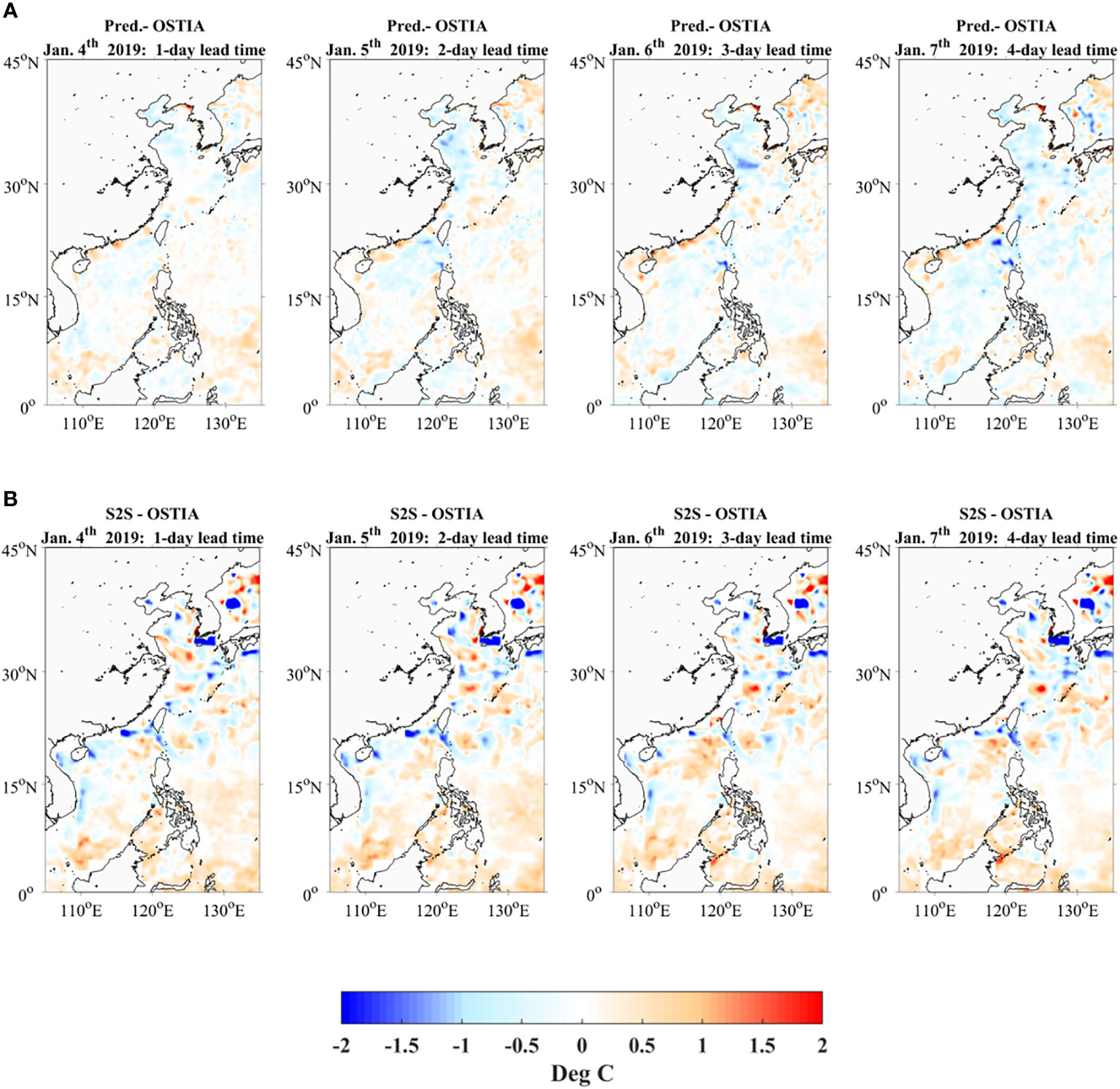
Figure 6 The spatial distribution of SST difference between (A) predicted SSTs and OSTIA and (B) S2S and OSTIA from January 4th to 10th, 2019.
4. Conclusions
The 3DConv-LSTM model is proposed to predict daily SSTs with a 1- to 7-day lead time and a 0.05° spatial resolution in the China Seas and their adjacent waters. The model’s prediction ability was assessed via comparing to the OSTIA test dataset, the S2S data, and the near-surface Argo data from 2015 to 2019.
There is good agreement between predicted SSTs and the OSTIA test dataset within a 1-to 3-day lead time, with 5-year RMSE between prediction and OSTIA are 0.27°C, 0.35°C and 0.41 °C, respectively. With a 3- to 7-day lead time, the RMSE drops from 0.41 °C to 0.53 °C. Since only the SSTA sequences are used for training data, the model prediction ability is related to the temporal correlation of global SST. During the testing period, the model shows a stable prediction ability. An increase of standard deviation errors occurs in areas of high SST variability. If computational resources are sufficient, separate models can be constructed for sub-regions with high SST variability to improve prediction accuracy. A comparison between the prediction-minus-Argo and the S2S-minus-Argo shows that the model has a slightly higher prediction accuracy with a 1- to 3-day lead time. In 4- to 7-day lead time, their prediction ability is similar. However, the S2S has more stable standard deviation errors and may in part include more ensemble members. The results presented here indicate that the DL-based model is accurate and reliable and can be applied in regional daily SST prediction.
Data availability statement
The original contributions presented in the study are included in the article/supplementary material. Further inquiries can be directed to the corresponding author.
Author contributions
LW developed the methodology, calculations, analyzed the data, and written the initial manuscript. LG provided assistance in manuscript review and data validation. All authors contributed to the article and approved the submitted version.
Funding
This work was supported by the National Key R&D Program of China (No. 2022YFC3104900), the National Natural Science Foundation of China (No.42206176), the Hainan Provincial Natural Science Foundation of China (No. 122CXTD519) and the 2022 Research Program of Sanya Yazhou Bay Science and Technology City (No.SKJC-2022-01-001).
Acknowledgments
The OSTIA SST data were provided by the Copernicus Marine Environment Monitoring Service. The Argo in situ data were provided by the iQuam System developed by the National Oceanic and Atmospheric Administration. The original S2S database is hosted at ECMWF as an extension of the TIGGE database.
Conflict of interest
The authors declare that the research was conducted in the absence of any commercial or financial relationships that could be construed as a potential conflict of interest.
Publisher’s note
All claims expressed in this article are solely those of the authors and do not necessarily represent those of their affiliated organizations, or those of the publisher, the editors and the reviewers. Any product that may be evaluated in this article, or claim that may be made by its manufacturer, is not guaranteed or endorsed by the publisher.
References
Aguilar-Martinez S., Hsieh W. W. (2009). Forecasts of tropical pacific sea surface temperatures by neural networks and support vector regression. Int. J. Oceanography 2009:(167239), 1–13. doi: 10.1155/2009/167239
Aparna S., D’souza S., Arjun N. B. (2018). Prediction of daily sea surface temperature using artificial neural networks. Int. J. Remote Sens. 39 (12), 4214–4231. doi: 10.1080/01431161.2018.1454623
Boukabara S. A., Stewart J. Q., Maddy E. S., Shahroudi N., Hoffman R. N. (2019). Leveraging modern artificial intelligence for remote sensing and NWP: Benefits and challenges. Bull. Am. Meteorological Soc. 100 (12), ES473–ES491. doi: 10.1175/BAMS-D-18-0324.1
Donlon C. J., Martin M., Stark J., Roberts-Jones J., Fiedler E., Wimmer W. (2012). The operational sea surface temperature and sea ice analysis (OSTIA) system. Remote Sens. Environ. 116, 140–158. doi: 10.1016/j.rse.2010.10.017
Garcia-Gorriz E., Garcia-Sanchez J. (2007). Prediction of sea surface temperatures in the western Mediterranean Sea by neural networks using satellite observations. Geophysical Res. Lett. 34 (L11603), 1–6. doi: 10.1029/2007GL029888
Hochreiter S., Schmidhuber J. (1997). Long short-term memory. Neural Comput. 9 (8), 1735–1780. doi: 10.1162/neco.1997.9.8.1735
Hosoda K., Kawamura H. (2004). Global space-time statistics of sea surface temperature estimated from AMSR-e data. Geophysical Res. Lett. 31 (17), 345–359. doi: 10.1029/2004GL020317
Hsieh W. W. (2001). Nonlinear canonical correlation analysis of the tropical pacific climate variability using a neural network approach. J. Climate 14 (12), 2528–2539. doi: 10.1175/1520-0442(2001)014<2528:NCCAOT>2.0.CO;2
IOCCG (2009). Remote sensing in fisheries and aquaculture (Reports of the international ocean-colour coordinating group, no. 8) (Dartmouth, NS: International Ocean-Colour Coordinating Group (IOCCG). doi: 10.25607/OBP-98r
Ji S., Xu W., Yang M., Yu K. (2012). 3D convolutional neural networks for human action recognition. IEEE Trans. Pattern Anal. Mach. Intell. 35 (1), 221–231. doi: 10.1109/TPAMI.2012.59
Kamangir H., Krell E., Collins W., King S., PTissot P. (2022). Importance of 3D convolution and physics on a deep learning coastal fog model. Environ. Model. Software 154, 105424. doi: 10.1016/j.envsoft.2022.105424
Li W., Daniel J., Leonardo D. (1996). Predictions of Sea surface temperature in tropical ocean using neural networks. An. Acad. Bras. Ciências 68, 23–33.
Li X., Liu B., Zheng G., Ren Y., Zhang S., Liu Y., et al. (2020). Deep learning-based information mining from ocean remote sensing imagery. Natl. Sci. Rev. 7(10), 1584–1605. doi: 10.1093/nsr/nwaa047
Liu G., Rauenzahn J. L., Heron S. F., Eakin C. M., Skirving W. J., Christensen T., et al. (2013) NOAA Coral reef watch 50 km satellite sea surface temperature-based decision support system for coral bleaching management. Available at: https://repository.library.noaa.gov/view/noaa/743.
Mahongo S. B., Deo M. C. (2013). Using artificial neural networks to forecast monthly and seasonal sea surface temperature anomalies in the western Indian ocean. Int. J. Ocean Climate Syst. 4 (2), 133–150. doi: 10.1260/1759-3131.4.2.133
McLaren A., Fiedler E., Roberts-Jones J., Martin M. (2014). Quality information document (SST-GLO-SST-L4-REP-OBSERVATIONS-010-011) (EU Copernicus Marine Service). Available at: https://catalogue.marine.copernicus.eu/documents/QUID/CMEMS-OSI-QUID-010-011.pdf
McLaren A., Fiedler E., Roberts-Jones J., Martin M., Mao C. Y., Good S. (2021). Quality information document (SST-GLO-SST-L4-NRT-OBSERVATIONS-010-001) (EU Copernicus Marine Service). Available at: https://catalogue.marine.copernicus.eu/documents/QUID/CMEMS-SST-QUID-010-001.pdf.
McTaggart-Cowan R., Davies E. L., Fairman J. G. Jr., Galarneau T. J. Jr., Schultz D. M. (2015). Revisiting the 26.5° c sea surface temperature threshold for tropical cyclone development. Bull. Am. Meteorological Soc. 96 (11), 1929–1943. doi: 10.1175/BAMS-D-13-00254.1
Patil K., Deo M. C. (2017). Prediction of daily sea surface temperature using efficient neural networks. Ocean Dynamics 67 (3-4), 357–368. doi: 10.1080/01431161.2018.1454623
Patil K., Deo M. C., Ghosh S., Ravichandran M. (2013). Predicting sea surface temperatures in the north Indian ocean with nonlinear autoregressive neural networks. Int. J. Oceanography 2013 (302479), 1–11. doi: 10.1155/2013/302479
Patil K., Deo M. C., Ravichandran M. (2016). Prediction of sea surface temperature by combining numerical and neural techniques. J. Atmospheric Oceanic Technol. 33 (8), 1715–1726. doi: 10.1175/JTECH-D-15-0213.1
Patil K. R., Iiyama M. (2022). Deep learning models to predict Sea surface temperature in tohoku region. IEEE Access 10, 40410–40418. doi: 10.1109/ACCESS.2022.3167176
Qiao B., Wu Z., Tang Z., Wu G. (2021). “Sea Surface temperature prediction approach based on 3D CNN and LSTM with attention mechanism,” in 2021 23rd International Conference on Advanced Communication Technology (ICACT). (PyeongChang: IEEE). 342–347. doi: 10.23919/ICACT51234.2021.9370514
Roberts-Jones J., Fiedler E. K., Martin M. J. (2012). Daily, global, high-resolution SST and sea ice reanalysis for 1985–2007 using the OSTIA system. J. Climate 25 (18), 6215–6232. doi: 10.1175/JCLI-D-11-00648.1
Roxanne L. (2016). Exploring the future of marine farming in new Zealand under climate change conditions: using sea surface temperature (Canterbury: Lincoln University).
Shao Q., Li W., Han G. J., Hou G. C., Liu S. Y., Gong Y. T., et al. (2021). A deep learning model for forecasting Sea surface height anomalies and temperatures in the south China Sea. J. Geophysical Research-Oceans 126, 18. doi: 10.1029/2021JC017515
Taieb S. B., Bontempi G., Atiya A. F., Sorjamaa A. (2012). A review and comparison of strategies for multi-step ahead time series forecasting based on the NN5 forecasting competition. Expert Syst. Appl. 39 (8), 7067–7083. doi: 10.1016/j.eswa.2012.01.039
Tangang F., Hsieh W. W., Tang B. (1997). Forecasting the equatorial pacific sea surface temperatures by neural network models. Climate Dynamics 13 (2), 135–147. doi: 10.1007/s003820050156
Tangang F. T., Hsieh W. W., Tang B. (1998a). Forecasting regional sea surface temperatures in the tropical pacific by neural network models, with wind stress and sea level pressure as predictors. J. Geophysical Research: Oceans 103 (C4), 7511–7522. doi: 10.1029/97JC03414
Tangang F. T., Tang B., Monahan A. H., Hsieh W. W. (1998b). Forecasting ENSO events: A neural network–extended EOF approach. J. Climate 11 (1), 29–41. doi: 10.1175/1520-0442(1998)011<0029:FEEANN>2.0.CO;2
Tang B., Hsieh W. W., Monahan A. H., Tangang F. T. (2000). Skill comparisons between neural networks and canonical correlation analysis in predicting the equatorial pacific sea surface temperatures. J. Climate 13 (1), 287–293. doi: 10.1175/1520-0442(2000)013<0287:SCBNNA>2.0.CO;2
Vitart F., Ardilouze C., Bonet A., Brookshaw A., Chen M., Codorean C., et al. (2017). The subseasonal to seasonal (S2S) prediction project database. Bull. Am. Meteorological Soc. 98 (1), 163–173. doi: 10.1175/BAMS-D-16-0017.1
Wei L., Guan L., Qu L. (2019). Prediction of Sea surface temperature in the south China Sea by artificial neural networks. IEEE Geosci. Remote Sens. Lett. 99), 1–5. doi: 10.1109/LGRS.2019.2926992
Wei L., Guan L., Qu L., Guo D. (2020). Prediction of Sea surface temperature in the China seas based on long short-term memory neural networks. Remote Sens. 12 (17), 2697. doi: 10.3390/rs12172697
Woo H.-J., Park K. (2020). Inter-comparisons of daily sea surface temperatures and in-situ temperatures in the coastal regions. Remote Sens. 12, 1592. doi: 10.3390/rs12101592
Wu A., Hsieh W. W., Tang B. (2006). Neural network forecasts of the tropical pacific sea surface temperatures. Neural Networks 19 (2), 145–154. doi: 10.1016/j.neunet.2006.01.004
Xiao C., Chen N., Hu C., Wang K., Xu Z., Cai Y., et al. (2019). A spatiotemporal deep learning model for sea surface temperature field prediction using time-series satellite data. Environ. Model. Software 120, 104502. doi: 10.1016/j.envsoft.2019.104502
Xie J., Zhu J., Li Y. (2008). Assessment and inter-comparison of five high-resolution sea surface temperature products in the shelf and coastal seas around China. Continental Shelf Res. 28, 1286–1293. doi: 10.1016/j.csr.2008.02.020
Xu L., Li Y., Yu J., Li Q., Shi S. (2020). Prediction of sea surface temperature using a multiscale deep combination neural network. Remote Sens. Lett. 11 (7), 611–619. doi: 10.1080/2150704X.2020.1746853
Yang Y., Dong J., Sun X., Lima E., Mu Q., Wang X. (2017). A CFCC-LSTM model for sea surface temperature prediction. IEEE Geosci. Remote Sens. Lett. 15 (2), 207–211. doi: 10.1016/j.envsoft.2019.104502
Yu X., Shi S. X., Xu L. Y., Liu Y. Y., Miao Q. S., Sun M. (2020). A novel method for Sea surface temperature prediction based on deep learning. Math. Problems Eng. 2020, 9. doi: 10.1155/2020/6387173
Zhang C., Feng Z., Zhang X., Zhang Q. (2017). Analysis on research progress of kuroshio. World Sci-tech R&D 39 (3), 239–249. doi: 10.16507/j.issn.1006-6055.2017.03.002
Zhang Z., Pan X., Jiang T., Sui B., Liu C., Sun W. (2020). Monthly and quarterly Sea surface temperature prediction based on gated recurrent unit neural network. J. Mar. Sci. Eng. 8 (4), 249. doi: 10.3390/jmse8040249
Keywords: Long short-term memory, operational SST and sea ice analysis (OSTIA), sea surface temperature (SST), spatiotemporal prediction, three-dimensional convolution
Citation: Wei L and Guan L (2022) Seven-day sea surface temperature prediction using a 3DConv-LSTM model. Front. Mar. Sci. 9:905848. doi: 10.3389/fmars.2022.905848
Received: 28 March 2022; Accepted: 29 November 2022;
Published: 16 December 2022.
Edited by:
Elodie Claire Martinez, UMR6523 Laboratoire d'Oceanographie Physique et Spatiale (LOPS), FranceReviewed by:
Ming Feng, Commonwealth Scientific and Industrial Research Organisation (CSIRO), AustraliaShuohao Li, National University of Defense Technology, China
Copyright © 2022 Wei and Guan. This is an open-access article distributed under the terms of the Creative Commons Attribution License (CC BY). The use, distribution or reproduction in other forums is permitted, provided the original author(s) and the copyright owner(s) are credited and that the original publication in this journal is cited, in accordance with accepted academic practice. No use, distribution or reproduction is permitted which does not comply with these terms.
*Correspondence: Lei Guan, bGVpZ3VhbkBvdWMuZWR1LmNu