 Zineng Yuan
 John K. Keesing2
- 1Deep-Sea Multidisciplinary Research Center, Qingdao National Laboratory for Marine Science and Technology, Qingdao, China
- 2Commonwealth Scientific and Industrial Research Organisation, (CSIRO) Oceans and Atmosphere Research, Crawley, Australia and School of Molecular and Life Sciences, Curtin University, Bentley, WA, Australia
- 3State Key Laboratory of Estuarine and Coastal Research, East China Normal University, Shanghai, China
The overlapping effect of anthropogenic activities and climate change are major drivers for a shift in coastal marine phytoplankton biomass. Linear regression analyses are not sufficient to detect the nonlinear relationship between complex environmental factors and phytoplankton shift. Here, an Artificial Neural Network (ANN) model is applied to quantify the relative contribution of pearl oyster farming, temperature and rainfall on phytoplankton increases in Cygnet Bay, Australia. The result shows that increased oyster farming ranks among the most important factors for phytoplankton increases, with a relative importance of 54% for diatoms and 74% for dinoflagellates; temperature plays a second important role with a positive impact on diatoms (relative importance of 25%) but a negative impact on dinoflagellates (relative importance of 19%); rainfall is the least important which enhances diatom biomass only (relative importance of 21%). Our ANN analysis provides a useful approach for quantifying the complex interrelationships affecting phytoplankton shift.
Introduction
Over the past several decades, coastal phytoplankton has been facing strong and rapid changes forced by a combination of human activities and climate change (Boyce et al., 2010; Cloern and Jassby, 2010). Nutrient enrichment caused by aquaculture, coastal development and pollution are just a few of the many ways humans impact coastal seas altering phytoplankton dynamics (Liu et al., 2013; Glibert, 2020). Meanwhile, climate-driven changes in temperature, precipitation and large-scale climate patterns can have major consequences for phytoplankton through changes in hydrologic conditions or macronutrient concentrations (Lewandowska et al., 2014; Thompson et al., 2015; Lin et al., 2020). In general, it is thought that climate change will result in a decrease in marine phytoplankton productivity as ocean warming enhances stratification, reducing nutrient supply to the upper ocean (Behrenfeld et al., 2006; Boyce et al., 2010). However, the situation tropical coastal seas may well be different with changes to rainfall patterns and cyclone frequency and intensity, coastal land use and even wildfires, resulting in increased nutrient inputs which enhance coastal phytoplankton productivity (Yuan et al., 2020; Liu et al., 2022). Understanding how these multiple environmental variables have influenced phytoplankton in the past is fundamental for the prediction of future changes, and to help develop policies for ecosystem health (Levin et al., 2015).
Paleoecological analysis of geochemical proxies in the sediments is increasingly being applied to investigate and interpret environmental changes, due to its high efficiency to acquire long-term ecological records (Smittenberg et al., 2004; Xing et al., 2016; Yuan et al., 2018). Most of these studies have assumed a simple linear relationship between environmental factors and phytoplankton, and attributed to the most relevant factor via straightforward visual inspection or linear regression analyses. However, the complex nature of phytoplankton dynamics, in particular multivariate (Irwin et al., 2012; Mutshinda et al., 2013) and nonlinearity (Jochimsen et al., 2012; Feng et al., 2021), make traditional statistical tools such as Pearson correlation analysis and Principal component analysis (PCA) difficult to explain all the complex interrelationships affecting phytoplankton dynamics. There is an imperative to apply more elaborate methods to better understand the complex relationship between the environmental forces and phytoplankton response. Artificial Neural Network (ANN) is a type of machine learning algorithm inspired by the functioning of the brain and nervous system (Rumelhart et al., 1986). The capability of approximating nonlinear multivariate functions with high accuracy and stability makes them particularly suitable to solve complex ecological problems (Gevrey et al., 2003). This approach has been proved to attain better performance than traditional linear statistical tools (Maravelias et al., 2003) and successfully applied to solve a range of relation recognition problems from landscape (Buckland et al., 2019) to microbial community (Santos et al., 2014). Specifically for phytoplankton research, ANNs have been applied in different aquatic environments such as rivers (Jeong et al., 2006), lakes (Li et al., 2007), estuaries (Coutinho et al., 2019), and open ocean (Mattei & Scardi, 2020) to understand the influence of different environmental factors on phytoplankton.
The Kimberley coast, tropical Australia (Figure 1), is a remote region with a small population living in small townships spread of a very large area, but is undergoing increasing pressures from anthropogenic activities and climate variability (Lough, 2008; O’Donnell et al., 2015). Field observations and paleoecological data suggested that significant increases in phytoplankton productivity have occurred over the past several decades (Furnas & Carpenter, 2016; Liu et al., 2016; Yuan et al., 2018). Most evidence demonstrated that climate-induced changes in temperature and rainfall were the dominant drivers because warming directly affected phytoplankton metabolic rates, and rainfall associated with increased tropical cyclones can enhance nutrient supply (Yuan et al., 2018; Yuan et al., 2020). In addition, nutrient enrichment from mariculture (Liu et al., 2016), seasonal urban runoff and contaminated groundwater inputs (Estrella et al., 2011; Gunaratne et al., 2017) can elevate phytoplankton production significantly at the local scale. It is acknowledged that multiple factors may jointly increase phytoplankton biomasses in this region, however, the effects of each driver still lack quantitative assessment. The climatic factors, temperature and rainfall, and anthropogenic history are significantly correlated and so estimated effects will also be correlated. Ideally, a process-based ecological model would be used to simulate phytoplankton responses to climatic and anthropogenic stressors. However, these mechanistic models are not yet established in the Kimberley coast. Therefore, the data-driven empirical approach of ANN analysis would be highly useful, considering its strong capability to unravel the complex relationships between ecological variables.
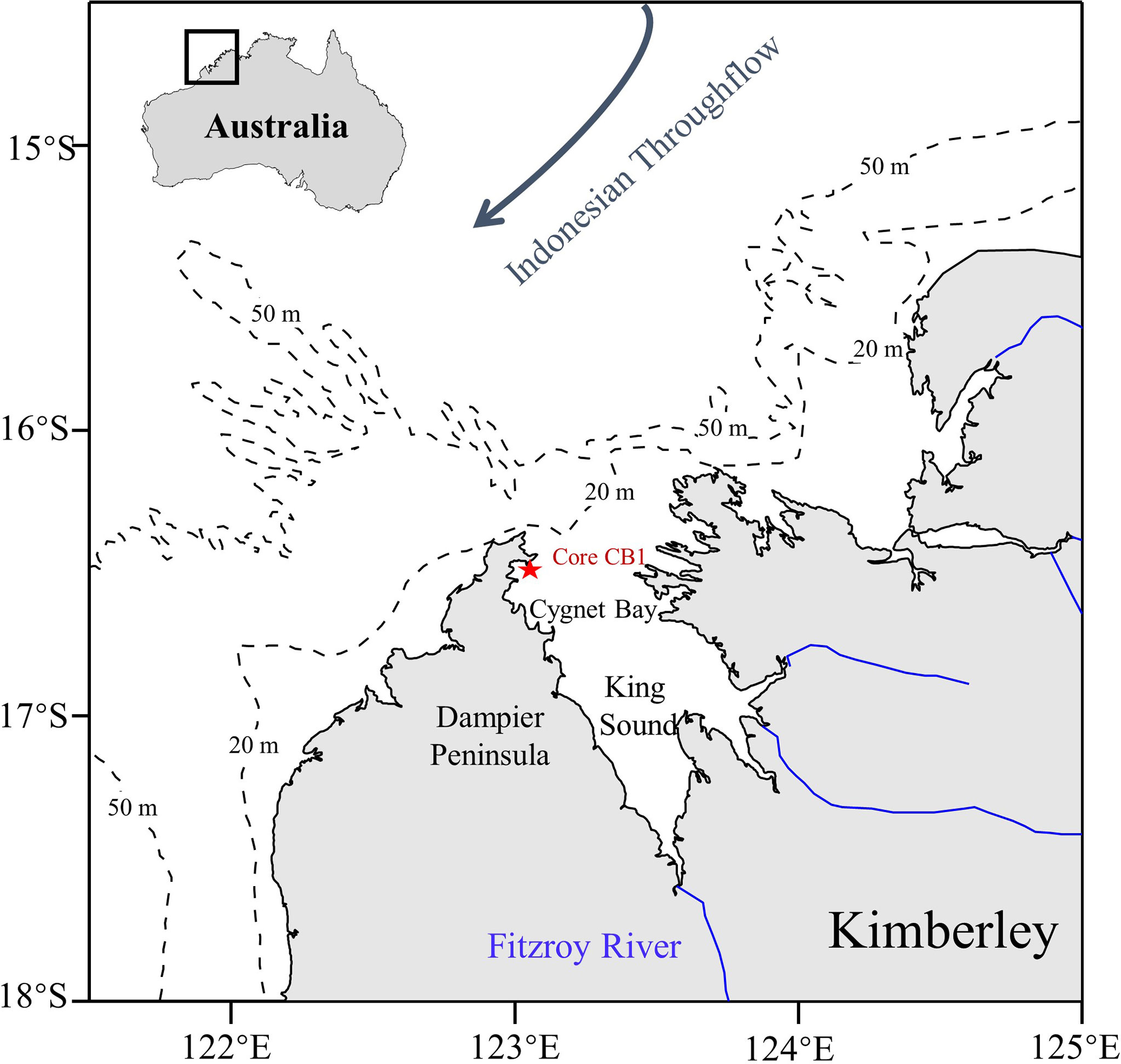
Figure 1 A schematic map showing the sampling sites * Core CB1) along the Kimberley coastline in North-Western Australia.
In this study, we explored the potential for novel applications of machine learning techniques (ANN) to improve our understanding of the relationship between climatic and anthropogenic disturbances and long-term phytoplankton changes. Firstly, we analyzed four biomarker proxies (TEX86H index, long-chain n-alkanes, brassicasterol, and dinosterol) in the sediment core obtained from Cygnet Bay by Liu et al. (2016) to reconstruct the records of Sea Surface Temperature (SST), rainfall, and the diatom and dinoflagellate biomasses, respectively. The applications of these biomarker proxies in coastal waters of north-western Australia have been validated by previous studies (Burns et al., 2003; Yuan et al., 2018). Then, an ANN model was built with the paleoecological data and collected historical archives. This ANN model was carefully validated to ensure that it could provide accurate results without biases or overfitting. We demonstrate the use of the ANN model to quantify the relative importance of pearl oyster farming, SST and rainfall for diatom and dinoflagellate changes during the past century.
Materials and Methods
Core Information
The core used in this study was from Liu et al. (2016) collected by SCUBA divers in 2011. Liu et al. (2016) chose two sites, with one site under the direct influence of pearl oyster farming and the other a reference site 1.5 km away from pearl oyster farming and aimed to understand the impact of pearl oyster farming on the sediment quality in Cygnet Bay. Chronology and geochemical parameters including total organic matter, carbon and nitrogen isotopes, and C/N were analyzed in both sites (Liu et al., 2016). A subsequent study by Yuan et al. (2018) chose the reference site and analyzed biomarker proxies including TEX86, long-chain n-alkanes, brassicasterol, and dinosterol. They aimed to verify the applicability of the biomarker proxies and to investigate the climate effects on phytoplankton in Cygnet Bay. Here, we used the unpublished biomarker data from the pearl oyster farming site (Core CB1, 16° 28’ S, 123° 02’ E, depth: 11.5 m; Figure 1) to further understand the different role of pearl oyster farming and climate factors driving phytoplankton changes. The chronology of Core CB1 was cited from Liu et al. (2016), which generated a sedimentation rate of 1.11 cm yr-1, covering a time span of approximately 1910-2011.
Biomarker Analysis
The core was sectioned at 1 cm intervals. Then, the subsamples were extracted with dichloromethane/MeOH, and the neutral lipids were extracted with hexane and separated into two fractions using silica gel chromatography. The nonpolar lipid fraction was eluted with hexane, and the polar lipid fraction was eluted with dichloromethane/methanol. Subsequently, the polar fraction was divided into two parts, one derivatized using N, O-bis(trimethylsilyl)-trifluoroacetamide (BSTFA) and the other filtered by PTFE membrane (0.45 μm). The long-chain n-alkanes, brassicasterol, and dinosterol were quantified by GC (Agilent 6890N) with an FID detector. Glycerol Dialkyl Glycerol Tetraethers (GDGTs) analysis was performed by HPLC-MS (Agilent 1200/Waters Micromass-Quattro UltimaTM Pt) with APCI probe and Prevail Cyano Column.
The TEX86H index was calculated based on the relative abundance of GDGTs defined by Kim et al. (2010) (Eq. 1) and converted into SST according to the global equation (Eq. 2) (Kim et al., 2010).
where H stood for high temperature regions, the numbers 1-3 indicated the number of cyclopentane rings in GDGTs and Cren’ was the regioisomer of crenarchaeol.
The long-chain n-alkanes (C27 + C29 + C31), specific to higher land plants, were widely used to access the impact of terrestrial input in marine sediments in terms of changes in rainfall, river discharge or dust input (Eglinton & Hamilton, 1967; Seki et al., 2003). A previous paper in Cygnet Bay have compared the down-core variations of long-chain n-alkanes with rainfall as well as the river discharge, and they found very similar increasing patterns (Yuan et al., 2018). The increasing trend of long-chain n-alkane in Core CB1 also matched well with the instrumental rainfall observations (Figure S1). Thus, we used long-chain n-alkanes to represent rainfall (terrestrial influence) in this study.
Data Source and Statistical Analysis
The practice of the pearl industry in Western Australia has typically involved two steps: first, wild pearl oysters Pinctada maxima with appropriate sizes were collected by fishing vessels in shallow coastal waters; second, the collected pearl oysters were cultured to produce pearls in pearl farms. The pearl production and pearl farm size were closely related to the annual caught numbers of wild pearl oyster shells (Fletcher et al., 2006). The Brown family, who own and manage Cygnet Bay Pearls, started farming in 1960 at low density; the farm size and stock level expanded rapidly since modern long-line culture established in the 1980s (www.cygnetbaypearlfarm.com.au/; also see Liu et al., 2016). These changes show an excellent coincidence with the total pearl oyster catch in the Broome area from 1960 to 2011 (Figure 2E; data obtained from the Department of Primary Industries and Regional Development; www.fish.wa.gov.au). Despite being a quota managed fishery, generally, pearl oyster catch is regarded as a good indicator the scale of pearl farming activity despite some fluctuations in demand for wild shell driven by hatchery produced shell supplementing wild caught shell from the mid-1990s to 2006 (when disease affected hatchery production) and the 2008 global financial crisis affecting demand for pearls (James Brown, Cygnet Bay Pearls, personal communication). Thus, we used pearl oyster catch numbers in the Broome area to represent the farming intensity in Cygnet Bay. The data from 1960 to 1978 was collected with catch weight (tonne). To keep consistency, we calculated the catch number for this period by assuming an average weight of 1 kg per pearl oyster.
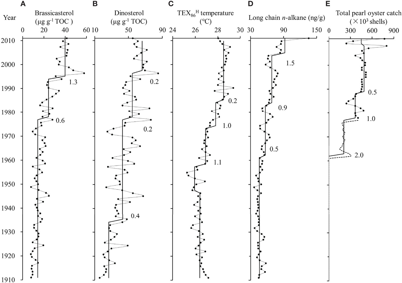
Figure 2 Profiles of TOC normalized brassicasterol and dinosterol contents (A, B), TEX86H temperature (C), long chain n-alkane contents (D), and total pearl oyster catch (E). The solid lines show shift trends assessed by sequential t test analysis of regime shift and numbers are regime shift index. Significant level is set to p< 0.05. The dashed line in total pearl oyster catch is calculated by assuming an average weight of 1 kg for each pearl oyster.
Interpolation analysis used Origin 8.0 software (mathematics: interpolate) to reduce asynchronous errors between sediment records and collected historical archives. Pearson correlation analysis and principle component analysis (PCA) used SPSS 16 (Statistical Package for the Social Sciences Inc.) to detect linear correlations between phytoplankton biomass and environmental variables. The sequential t test analysis of regime shifts (STARS; www.BeringClimate.noaa.gov) (Rodionov, 2004; Rodionov and Overland, 2005) was written in VBA for Microsoft Excel to detect the timing and magnitude of the shift changes in each record. The cutoff length (l) was set to 10 with a significant level of 5%.
Artificial Neural Network (ANN) Model
A typical ANN’s structure consists of 3 interconnected layers: an input layer, one or more hidden layers, and an output layer, with each layer containing one or more neurons (Supplementary Figure S2). The neurons are connected with the next layer neurons with adjustable weights and each connection represents one computation. During training, the weights are adjusted over each iteration towards values that can minimize the errors between calculated output and actual output. This procedure is repeated until the errors become small enough. A more detailed description can be found in Coutinho et al. (2019) and Krogh and Anders (2008).
We carried out ANN analyses in the R environment version 4.1.1 (R Core Team, 2021). The ‘nnet’ function from package ‘nnet’ (Ripley et al., 2016) was used to train networks. The ‘garson’ and ‘olden’ functions from package ‘NeuralNetTools’ (Beck, 2018) were used for importance analysis. The ‘lek profile’ function from package ‘NeuralNetTools’ was used for sensitivity analysis. A three-layer ANN was built with three input neurons (pearl oyster farming, SST and rainfall), one hidden neuron and two output neurons (diatom and dinoflagellate abundances) (Supplementary Figure S2). We chose pearl oyster farming, SST and rainfall as the input variables in the ANN model because they were explicitly suggested as the main drivers for phytoplankton changes in this region (Liu et al., 2016; Yuan et al., 2018; Yuan et al., 2020). The pearl oyster farming activities were assumed zero before it was established in 1960. All input and output data during the period from 1910 to 2011 were normalized by scaling it into the [0, 1] interval and randomly divided into the training and validation samples prior to training. ANN performance was evaluated by calculating the Pearson Correlation Coefficients for training (PCCt) and validation (PCCv) samples and the Root Mean Square Errors for training (RMSEt) and validation samples (RMSEv). High PCC (>0.5) and low RMSE values (<1) for both training and validation samples indicated that networks were considered valid. To achieve the best performance of ANN networks without overfitting, these networks were carefully validated following Coutinho et al. (2019). Briefly, ANN was tested with different numbers of hidden neurons (from 1 to 10), training iterations (from 2 to 1024) and percentage of samples used for training (from 5% to 95%). One hundred networks were trained for each combination of parameters. We found no evidence that the changing hidden neurons and percentage of samples used for training will influence the network performance (Supplementary Figures S3, S4). The networks with training iterations above 32 produced comparable PCCt and RMSEt as well as PCCv and RMSEv values (Supplementary Figure S5). Thus, we built the final ANN using the parameters as follows: hidden neuron was set to 1; samples were randomly and evenly divided into training and validation sets; maximum number of iterations was set to 1000; reltol was set to 0.01; and weight decay was set to 0.001. Then, we proceeded to put all data (n = 91) for training and selected the network with the lowest RMSEt as the best network. Finally, the relative importance of the input variables was estimated in the best network based on the ‘Olden’ method (Olden et al., 2004). This approach calculated the summed product of connection weights between each input-hidden neuron connection and hidden-output neuron connection. The positive values indicated that the input variable had a positive association with the output variable, and the negative values indicated the input variable had a negative association with the output variable. A sensitivity test was also performed in the best network to understand how each input variable individually influenced the output variables. The output variables were modelled with changing one input variable at a time, while all the other input variables were held constant at their 10th, 30th, 50th, 70th and 90th percentile values (Supplementary Figure S6).
Results
Temporal Patterns of Biomarker Proxies
The brassicasterol contents, representing diatom biomass in this study, varied from 7.7 to 57.7 μg g-1 TOC. They remained steady until the late-1970s and then showed two increasing shifts in 1978 and 1995 according to the STARS analysis (RSI: 0.6 and 1.3; Figure 2A). The dinosterol contents, representing dinoflagellate biomass, varied from 15.8 to 85.0 μg g-1 TOC. They displayed a gradual increasing pattern with three increasing shifts in 1935, 1978 and 1998 (RSI: 0.4, 0.2 and 0.2; Figure 2B).
A previous study validated the application of TEX86H index for SST reconstruction in Cygnet Bay (Yuan et al., 2018). In Core CB1, TEX86H temperature ranged from 25.3 to 29.4°C and displayed three different periods (Figure 2C): a low temperature period of 1900-1957 (average of 26.5°C), a warming period of 1957-1986 with three increasing shifts (RSI: 1.1, 1.0 and 0.2), and a high temperature period of 1986-2011 (average of 28.5°C). The contents of long-chain n-alkanes ranged from 36.5 to 135.5 ng g-1. They showed an increasing trend over time with three increasing shifts in 1961, 1983 and 2003 (RSI: 0.5, 0.9 and 1.5; Figure 2D). The historical archives showed that the pearl oyster farming industry in Cygnet Bay was first started in 1960 and intensified in the 1980s, which can be reflected in the total pearl oyster catch in the Broome area (Figure 2E).
correlation analysis showed that SST, rainfall and pearl oyster farming were significantly correlated with diatom and dinoflagellate biomasses (Table 1). Due to their close associations, PCA analysis failed to further distinguish the difference between each environmental factors and phytoplankton biomasses. Only one meaningful principal component, which accounted for 77.5% of the total variance, was extracted in the dataset containing the four biomarker proxies and pearl oyster farming history.
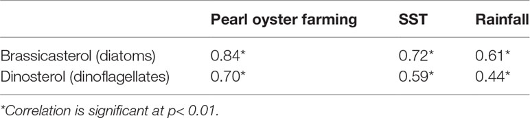
Table 1 Pearson correlation coefficients.
Relative Importance of Environmental Variable
The ANN model was successful in predicting the responses of diatoms and dinoflagellates. The best network displayed a PCC value of 0.86 and RMSE value of 0.11 for diatoms, and a PCC value of 0.75 and RMSE value of 0.15 for dinoflagellates. For both diatoms and dinoflagellates, pearl oyster farming consistently ranked as the most important factor, followed by SST, with rainfall the least important (Figures 3B, C). Pearl oyster farming was positively associated with diatoms and dinoflagellates with a relative importance of 54% for diatoms and 74% for dinoflagellates (Figure 3). SST had a positive association for diatoms with a relative importance of 25%, while had a negative association for dinoflagellates with a relative importance of 19% (Figure 3). Rainfall had a positive association with diatoms with a relative importance of 21% but was not as relevant with dinoflagellates (Figure 3).
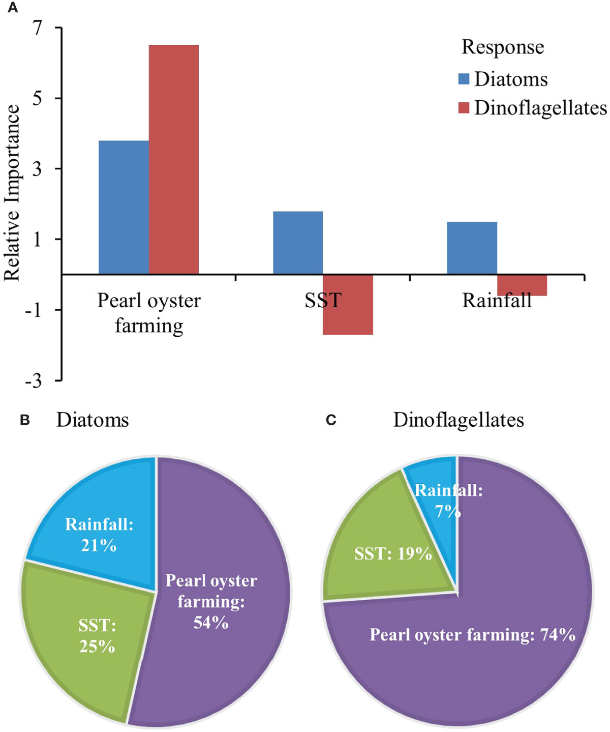
Figure 3 Bar (A) and pie plots (B, C) representing the relative importance of environmental factors for diatoms and dinoflagellates estimated from ANN weights through the ‘Olden’ method. The pie plots are calculated by the absolute values of the relative importance of environmental factors.
Discussion
Environmental Factors Influence Phytoplankton
In this study, diatom and dinoflagellate biomasses show significant increases in the 1970s and the 1990s (Figures 2A, B). The main drivers modulating phytoplankton can be approximately evaluated by linear statistical methods. Both Pearson correlation analysis and PCA analysis suggest that SST, rainfall and pearl oyster farming could contribute to the phytoplankton increases, but their separate effects cannot be distinguished. The ‘Olden’ method in the ANN enables visualization of the relative importance of each input variable and generates a number of new observations (Figure 3). The estimated relative importance shows that pearl oyster farming overwhelms SST and rainfall controls on diatom and dinoflagellate increases, which is consistent with current understanding. According to the total organic carbon and nitrogen records from the same site, there is a significant increase since the pearl oyster farming established in the 1960s; the δ13C, C/N and δ15N records indicate that the increased organic matter and nitrogen are mainly contributed by autochthonous sources, suggesting a more significant influence from pearl oyster farming than terrestrial input (Liu et al., 2016). A direct comparison of diatom records (biogenic silica) inside and outside the farming area also indicates that the impact of pearl oyster farming on diatom abundance is much greater than that of climate change (Liu et al., 2016). These lines of evidence are in agreement supporting that pearl oyster farming plays a dominant role in phytoplankton increases in Cygnet Bay.
Bivalve farming affects phytoplankton primarily through two distinct mechanisms (Forrest et al., 2009): bottom-up control of stimulating phytoplankton growth caused by nutrient remineralization in pseudofeces and feces (Sarà et al., 2011; Gallardi, 2014; Liang et al., 2019) and top-down control of depleting phytoplankton caused by bivalve grazing (Petersen et al., 2008; Jiang et al., 2019). The effect of bivalve grazing on phytoplankton may be most significant with a high stocking density of bivalve farming (Smaal et al., 2013) when decreasing bivalve biomass reaches a point at which the bottom-up effect begins to increase phytoplankton production. This process has been demonstrated in mesocosm (Prins et al., 1995) and field studies (Trottet et al., 2008; Sarà et al., 2011), both reveal enhanced phytoplankton abundances at low stocking density. The stocking density of pearl oysters in Cygnet Bay and other parts of north-western Australia is a very small size (<16 250 shells per square nautical mile) compared with other bivalve farming (Jelbart et al., 2011), hence, it can create a mutually beneficial environment for both phytoplankton and bivalve. The modern long-line culture in Cygnet Bay since the 1980s uses long line cages to suspend pearl oysters in waters. This culture method can reduce current speed significantly (Plew et al., 2005), which induces nutrient accumulation within the farming area and could also favor phytoplankton growth.
Temperature and rainfall are important determinants, but their influence markedly varies between diatoms and dinoflagellates (Figure 3A). Tropical phytoplankton used to have their optimum temperatures close to annual mean temperatures (Thomas et al., 2012). A small amount of warming can therefore easily exceed their optimum temperatures and lead to sharp declines in growth rate (Thomas et al., 2012). However, culture experiments demonstrate that evolutionary thermal adaptation can help phytoplankton to avoid the negative effect of warming, but this ability differs across phytoplankton species (Padfield et al., 2016; Thomas et al., 2016; Jin and Agustí, 2018). Several diatoms, particularly tropical species, can adapt to the warming environment rapidly by increasing their optimal temperature and maximum growth rate (Jin and Agustí, 2018; Schaum et al., 2018). Thus, the different adaptation capacities of diatoms and dinoflagellates could result in their opposite response to warming SST in Cygnet Bay. In common with previous studies (Yuan et al., 2018; Yuan et al., 2020), the ANN results also indicate that diatoms obtain greater benefits from increasing rainfall than dinoflagellates. This is because increasing rainfall not only brings rich silicate nutrients through river discharge but also creates turbulent conditions, both are better for diatom growth (Margalef, 1978; Irwin et al., 2012).
ANN Model for Palaeoecological Research
The application of palaeoecological data in ANN modeling allows us to combine the strength of both approaches. The palaeoecological approach is uniquely valuable in acquiring ecological data and assessing the impacts of environmental changes at supra-decadal timescales. As the raw data accumulate, the use of statistical models to advance our understanding of ecological dynamics is becoming increasingly important. Several conventional statistical approaches, including multiple linear regression (MLR) (Liu et al., 2022), principal component analysis (PCA) (Yuan et al., 2020), canonical correspondence analysis (CCA) (Liu et al., 2018) have been widely applied for a long time in palaeoecological studies. However, increasing evidence indicates that many ecological issues possess the characteristics of nonlinearity, time variation, and multiple forcing mechanisms (Andersen et al., 2009), and these conventional approaches to data analysis have presented limitations in revealing inner relationships and providing results prediction. The ANN methodology is capable to handle big data and complex nonlinear relationships; thus, it can make up for the inadequate understanding of mechanisms by using palaeoecological and conventional statistical approaches. The present study illustrates the feasibility and usefulness of neural networks in the field of palaeoecology; and it may prove promising to be applied to similar palaeoecological datasets from other ecosystems.
Despite the clear advantages, limitations of our ANN model still exist. For example, both sediment records and collected historical archives (pearl oyster catch numbers) are used as input data in our ANN model. There are asynchronous errors between the two different datasets, which could have hampered the ANN performance. Finding a pearl farming indicator in the sediment would be helpful to reduce this error. The model also did not incorporate some factors that likely influence phytoplankton dynamics such as nutrient structure (the ratio of macronutrients) (Burford et al., 2012; Armbrecht et al., 2015), tidal mixing and light variability (Mclaughlin et al., 2019; Mclaughlin et al., 2020). These factors are regarded as important drivers determining phytoplankton abundance in the modern Kimberley coast, but lack for an understanding of their historical changes as well as their impacts on phytoplankton in the past. In addition, the ANN model cannot be used to predict the values outside the range of training data. The model presented in this example is trained based on the palaeoecological data during the past century and is unable to predict how future phytoplankton under higher sea temperatures will change. Thus, the training dataset in the ANN model should cover as wide a range as possible to improve the predictable capabilities.
Conclusions
We have shown the capacity to use an ANN model coupled with paleoecological datasets to improve our understanding of anthropogenic and climatic factors driving long-term phytoplankton changes. The results in Cygnet Bay highlight that pearl oyster farming plays a dominant role for both diatoms and dinoflagellates increases, while climatic factors exert different influences between diatoms and dinoflagellates determined by their ecophysiological traits. Our ANN analysis may prove promising in solving complex paleoecological issues. Possible elaborations of this approach in future work will introduce more related environmental factors and incorporate more paleoecological data.
Data Availability Statement
The original contributions presented in the study are included in the article/Supplementary Material. Data used in this study are also publicly available at [https://doi.org/10.1594/PANGAEA.944532].
Author Contributions
ZY measured biomarker data and wrote the paper; JK designed the work and collected the sediment samples; DL conceived the idea and revised the manuscript; all authors contributed to improving the paper and approved the submitted version.
Funding
The study is funded by Natural Science Foundations of China (42030402, 41876127, 41641048), the Western Australian Marine Sciences Institution, Pilot National Laboratory for Marine Science and Technology (Qingdao) (Grant No. JCZX202001).
Conflict of Interest
The authors declare that the research was conducted in the absence of any commercial or financial relationships that could be construed as a potential conflict of interest.
Publisher’s Note
All claims expressed in this article are solely those of the authors and do not necessarily represent those of their affiliated organizations, or those of the publisher, the editors and the reviewers. Any product that may be evaluated in this article, or claim that may be made by its manufacturer, is not guaranteed or endorsed by the publisher.
Acknowledgments
We thank Yajun Peng for the analysis of TOC and chronology data, Honghua Shi and Yongzhi Liu for the establishment of the ANN model, Hailong Zhang and Li Li for biomarker technical support.
Supplementary Material
The Supplementary Material for this article can be found online at: https://www.frontiersin.org/articles/10.3389/fmars.2022.904461/full#supplementary-material
References
Andersen T., Carstensen J., Hernandez-Garcia E., Duarte C. M. (2009). Ecological Thresholds and Regime Shifts: Approaches to Identification. Trends Ecol. Evol. 24 (1), 49–57. doi: 10.1016/j.tree.2008.07.014
Armbrecht L. H., Thompson P. A., Wright S. W., Schaeffer A., Roughan M., Henderiks J., et al. (2015). Comparison of the Cross-Shelf Phytoplankton Distribution of Two Oceanographically Distinct Regions Off Australia. J. Mar. Syst. 148, 26–38. doi: 10.1016/j.jmarsys.2015.02.002
Beck M. W. (2018). NeuralNetTools: Visualization and Analysis Tools for Neural Networks. J. Stat. Softw 85 (11), 1. doi: 10.18637/jss.v085.i11
Behrenfeld M. J., O’Malley R. T., Siegel D. A., McClain C. R., Sarmiento J. L., Feldman G. C., et al. (2006). Climate-Driven Trends in Contemporary Ocean Productivity. Nature 444 (7120), 752–755. doi: 10.1038/nature05317
Boyce D. G., Lewis M. R., Worm B. (2010). Global Phytoplankton Decline Over the Past Century. Nature 466 (7306), 591–596. doi: 10.1038/nature09268
Buckland C., Bailey R., Thomas D. (2019). Using Artificial Neural Networks to Predict Future Dryland Responses to Human and Climate Disturbances. Sci. Rep. 9 (1), 1–13. doi: 10.1038/s41598-019-40429-5
Burford M. A., Webster I., Revill A., Kenyon R., Whittle M., Curwen G. (2012). Controls on Phytoplankton Productivity in a Wet-Dry Tropical Estuary. Estuar. Coast. Shelf S. 113, 141–151. doi: 10.1016/j.ecss.2012.07.017
Burns K. A., Volkman J. K., Cavanagh J.-A., Brinkman D. (2003). Lipids as Biomarkers for Carbon Cycling on the Northwest Shelf of Australia: Results From a Sediment Trap Study. Mar. Chem. 80 (2), 103–128. doi: 10.1016/S0304-4203(02)00099-3
Cloern J. E., Jassby A. D. (2010). Patterns and Scales of Phytoplankton Variability in Estuarine-Coastal Ecosystems. Estuar. Coast. 33 (2), 230–241. doi: 10.1007/s12237-009-9195-3
Coutinho F. H., Thompson C. C., Cabral A. S., Paranhos R., Dutilh B. E., Thompson F. L. (2019). Modelling the Influence of Environmental Parameters Over Marine Planktonic Microbial Communities Using Artificial Neural Networks. Sci. Total Environ. 677, 205–214. doi: 10.1016/j.scitotenv.2019.04.009
Eglinton G., Hamilton R. J. (1967). Leaf Epicuticular Waxes. Science 156 (3780), 1322. doi: 10.1126/science.156.3780.1322
Estrella S. M., Storey A. W., Pearson G., Piersma T. (2011). Potential Effects of Lyngbya Majuscula Blooms on Benthic Invertebrate Diversity and Shorebird Foraging Ecology at Roebuck Bay, Western Australia: Preliminary Results. J. R. Soc. Western Aust. 94 (2), 171–179.
Feng J., Stige L. C., Hessen D. O., Zuo Z., Zhu L., Stenseth N. C. (2021). A Threshold Sea-Surface Temperature at 14° C for Phytoplankton Nonlinear Responses to Ocean Warming. Glob. Biogeochem. Cycle 35 (5), e2020GB006808. doi: 10.1029/2020GB006808
Fletcher W., Friedman K., Weir V., McCrea J., Clark R. (2006). Pearl Oyster Fishery. ESD Report Series No. 5 (Western Australia: Department of Fisheries), 88 p.
Forrest B. M., Keeley N. B., Hopkins G. A., Webb S. C., Clement D. M. (2009). Bivalve Aquaculture in Estuaries: Review and Synthesis of Oyster Cultivation Effects. Aquaculture 298 (1-2), 1–15. doi: 10.1016/j.aquaculture.2009.09.032
Furnas M. J., Carpenter E. J. (2016). Primary Production in the Tropical Continental Shelf Seas Bordering Northern Australia. Cont. Shelf Res. 129, 33–48. doi: 10.1016/j.csr.2016.06.006
Gallardi D. (2014). Effects of Bivalve Aquaculture on the Environment and Their Possible Mitigation: A Review. Fish. Aquac. J. 5 (3), 105. doi: 10.4172/2150-3508.1000105
Gevrey M., Dimopoulos I., Lek S. (2003). Review and Comparison of Methods to Study the Contribution of Variables in Artificial Neural Network Models. Ecol. Model. 160 (3), 249–264. doi: 10.1016/S0304-3800(02)00257-0
Glibert P. M. (2020). Harmful Algae at the Complex Nexus of Eutrophication and Climate Change. Harmful Algae 91, 101583. doi: 10.1016/j.hal.2019.03.001
Gunaratne G. L., Vogwill R. I., Hipsey M. R. (2017). Effect of Seasonal Flushing on Nutrient Export Characteristics of an Urbanizing, Remote, Ungauged Coastal Catchment. Hydrolog. Sci. J. 62 (5), 800–817. doi: 10.1080/02626667.2016.1264585
Irwin A. J., Nelles A. M., Finkel Z. V. (2012). Phytoplankton Niches Estimated From Field Data. Limnol. Oceanograp. 57 (3), 787–797. doi: 10.4319/lo.2012.57.3.0787
Jelbart J. E., Schreider M., MacFarlane G. R. (2011). An Investigation of Benthic Sediments and Macrofauna Within Pearl Farms of Western Australia. Aquaculture 319 (3), 466–478. doi: 10.1016/j.aquaculture.2011.07.011
Jeong K. S., Kim D. K., Joo G. J. (2006). River Phytoplankton Prediction Model by Artificial Neural Network: Model Performance and Selection of Input Variables to Predict Time-Series Phytoplankton Proliferations in a Regulated River System. Ecol. Inform 1 (3), 235–245. doi: 10.1016/j.ecoinf.2006.04.001
Jiang Z., Du P., Liao Y., Liu Q., Chen Q., Shou L., et al. (2019). Oyster Farming Control on Phytoplankton Bloom Promoted by Thermal Discharge From a Power Plant in a Eutrophic, Semi-Enclosed Bay. Water Res. 159, 1–9. doi: 10.1016/j.watres.2019.04.023
Jin P., Agustí S. (2018). Fast Adaptation of Tropical Diatoms to Increased Warming With Trade-Offs. Sci. Rep. 8 (1), 17771. doi: 10.1038/s41598-018-36091-y
Jochimsen M. C., Kümmerlin R., Straile D., Grover J. (2012). Compensatory Dynamics and the Stability of Phytoplankton Biomass During Four Decades of Eutrophication and Oligotrophication. Ecol. Lett. 16 (1), 81–89. doi: 10.1111/ele.12018
Kim J., van der Meer J., Schouten S., Helmke P., Willmott V., Sangiorgi F., et al. (2010). New Indices and Calibrations Derived From the Distribution of Crenarchaeal Isoprenoid Tetraether Lipids: Implications for Past Sea Surface Temperature Reconstructions. Geochim. Cosmochim. Ac 74 (16), 4639–4654. doi: 10.1016/j.gca.2010.05.027
Krogh, Anders, (2008). What are Artificial Neural Networks? Nat. Biotechnol. 26 (2), 195. doi: 10.1038/nbt1386
Levin L. A., Liu K., Emeis K., Breitburg D. L., Cloern J., Deutsch C., et al. (2015). Comparative Biogeochemistry–Ecosystem–Human Interactions on Dynamic Continental Margins. J. Mar. Syst. 141, 3–17. doi: 10.1016/j.jmarsys.2014.04.016
Lewandowska A. M., Boyce D. G., Hofmann M., Matthiessen B., Sommer U., Worm B. (2014). Effects of Sea Surface Warming on Marine Plankton. Ecol. Lett. 17 (5), 614–623. doi: 10.1111/ele.12265
Liang Y., Zhang G., Wan A., Zhao Z., Wang S., Liu Q. (2019). Nutrient-Limitation Induced Diatom-Dinoflagellate Shift of Spring Phytoplankton Community in an Offshore Shellfish Farming Area. Mar. pollut. Bull. 141, 1–8. doi: 10.1016/j.marpolbul.2019.02.009
Li H., Hou G., Feng D., Xiao B., Song L., Liu Y. (2007). Prediction and Elucidation of the Population Dynamics of Microcystis Spp. In Lake Dianchi (China) by Means of Artificial Neural Networks. Ecol. Inform 2 (2), 184–192. doi: 10.1016/j.ecoinf.2007.03.007
Lin P., Ma J., Chai F., Xiu P., Liu H. (2020). Decadal Variability of Nutrients and Biomass in the Southern Region of Kuroshio Extension. Prog. Oceanog. 188, 102441. doi: 10.1016/j.pocean.2020.102441
Liu D., Peng Y., Keesing J. K., Wang Y., Richard P. (2016). Paleo-Ecological Analyses to Assess Long-Term Environmental Effects of Pearl Farming in Western Australia. Mar. Ecol. Prog. Ser. 552, 145–158. doi: 10.3354/meps11740
Liu D., Shen X., Di B., Shi Y., Keesing J. K., Wang Y., et al. (2013). Palaeoecological Analysis of Phytoplankton Regime Shifts in Response to Coastal Eutrophication. Mar. Ecol. Prog. Ser. 475, 1–14. doi: 10.3354/meps10234
Liu D., Wang Y., Wang Y., Keesing J. K. (2018). Ocean Fronts Construct Spatial Zonation in Microfossil Assemblages. Global Ecol. Biogeogr 27 (10), 1225–1237. doi: 10.1111/geb.12779
Liu D., Zhou C., Keesing J. K., Serrano O., Werner A., Fang Y., et al. (2022). Wildfires Enhance Phytoplankton Production in Tropical Oceans. Nat. Commun. 13 (1), 1348. doi: 10.1038/s41467-022-29013-0
Lough J. M. (2008). Shifting Climate Zones for Australia’s Tropical Marine Ecosystems. Geophys. Res. Lett. 35 (14), L14708. doi: 10.1029/2008GL034634
Maravelias C. D., Haralabous J., Papaconstantinou C. (2003). Predicting Demersal Fish Species Distributions in the Mediterranean Sea Using Artificial Neural Networks. Mar. Ecol. Prog. Ser. 255, 249–259. doi: 10.3354/meps255249
Margalef R. (1978). Life-Forms of Phytoplankton as Survival Alternatives in an Unstable Environment. Oceanol. ac 1 (4), 493–509.
Mattei F., Scardi M. (2020). Embedding Ecological Knowledge Into Artificial Neural Network Training: A Marine Phytoplankton Primary Production Model Case Study. Ecol. Model. 108985, 421. doi: 10.1016/j.ecolmodel.2020.108985
Mclaughlin M. J., Greenwood J., Branson P., Lourey M. J., Hanson C. E. (2020). Evidence of Phytoplankton Light Acclimation to Periodic Turbulent Mixing Along a Tidally Dominated Tropical Coastline. J. Geophys. Res. Oceans 125, e2020JC016615. doi: 10.1029/2020JC016615
Mclaughlin M. J., Lourey M. J., Hanson C. E., Cherukuru N., Thompson P. A., Pattiaratchi C. B. (2019). Biophysical Oceanography of Tidally-Extreme Waters of the Southern Kimberley Coast, Western Australia. Cont. Shelf Res. 173, 1–12. doi: 10.1016/j.csr.2018.12.002
Mutshinda C. M., Finkel Z. V., Irwin A. J. (2013). Which Environmental Factors Control Phytoplankton Populations? A Bayesian Variable Selection Approach. Ecol. Model. 269, 1–8. doi: 10.1016/j.ecolmodel.2013.07.025
O’Donnell A. J., Cook E. R., Palmer J. G., Turney C. S., Page G. F., Grierson P. F. (2015). Tree Rings Show Recent High Summer-Autumn Precipitation in Northwest Australia is Unprecedented Within the Last Two Centuries. PLos One 10 (6), e0128533. doi: 10.1371/journal.pone.0128533
Olden J. D., Joy M. K., Death R. G. (2004). An Accurate Comparison of Methods for Quantifying Variable Importance in Artificial Neural Networks Using Simulated Data. Ecol. Model. 178 (3-4), 389–397. doi: 10.1016/j.ecolmodel.2004.03.013
Padfield D., Yvon-Durocher G., Buckling A., Jennings S., Yvon-Durocher G., Hillebrand H. (2016). Rapid Evolution of Metabolic Traits Explains Thermal Adaptation in Phytoplankton. Ecol. Lett. 19 (2), 133–142. doi: 10.1111/ele.12545
Petersen J. K., Nielsen T. G., van Duren L., Maar M. (2008). Depletion of Plankton in a Raft Culture of Mytilus Galloprovincialis in Ría De Vigo, NW Spain. I. Phytoplankton. Aquat. Biol. 4 (2), 113–125. doi: 10.3354/ab00124
Plew D. R., Stevens C. L., Spigel R. H., Hartstein N. D. (2005). Hydrodynamic Implications of Large Offshore Mussel Farms. IEEE J. Oceanic Eng. 30 (1), 95–108. doi: 10.1109/JOE.2004.841387
Prins T. C., Escaravage V., Smaal A. C., Peeters J. C. H. (1995). Nutrient Cycling and Phytoplankton Dynamics in Relation to Mussel Grazing in a Mesocosm Experiment. Ophelia 41 (1), 289–315. doi: 10.1080/00785236.1995.10422049
R Core Team (2021). R: A Language and Environment for Statistical Computing. R Foundation for Statistical Computing, Vienna, Austria
Rodionov S. N. (2004). A Sequential Algorithm for Testing Climate Regime Shifts. Geophys. Res. Lett. 31 (9), L09204. doi: 10.1029/2004GL019448
Rodionov S. N., Overland J. E. (2005). Application of a Sequential Regime Shift Detection Method to the Bering Sea Ecosystem. Ices J. Mar. Sci. 62 (3), 328–332. doi: 10.1016/j.icesjms.2005.01.013
Rumelhart D. E., Hinton G. E., Williams R. J. (1986). Learning Representations by Back-Propagating Errors. Nature 323, 533–536. doi: 10.1038/323533a0
Santos E. C., Armas E. D., Crowley D., Lambais M. R. (2014). Artificial Neural Network Modeling of Microbial Community Structures in the Atlantic Forest of Brazil. Soil Biol. Biochem. 69 (1), 101–109. doi: 10.1016/j.soilbio.2013.10.049
Sarà G., Martire M. L., Sanfilippo M., Pulicanò G., Cortese G., Mazzola A., et al. (2011). Impacts of Marine Aquaculture at Large Spatial Scales: Evidences From N and P Catchment Loading and Phytoplankton Biomass. Mar. Environ. Res. 71 (5), 317–324. doi: 10.1016/j.marenvres.2011.02.007
Schaum C. E., Buckling A., Smirnoff N., Studholme D. J., Yvon-Durocher G. (2018). Environmental Fluctuations Accelerate Molecular Evolution of Thermal Tolerance in a Marine Diatom. Nat. Commun. 9 (1), 1719. doi: 10.1038/s41467-018-03906-5
Seki O., Kawamura K., Nakatsuka T., Ohnishi K., Ikehara M., Wakatsuchi M. (2003). Sediment Core Profiles of Long-Chain N-Alkanes in the Sea of Okhotsk: Enhanced Transport of Terrestrial Organic Matter From the Last Deglaciation to the Early Holocene. Geophys. Res. Lett. 30 (1), 1001. doi: 10.1029/2001GL014464
Smaal A., Schellekens T., Van Stralen M., Kromkamp J. (2013). Decrease of the Carrying Capacity of the Oosterschelde Estuary (SW Delta, NL) for Bivalve Filter Feeders Due to Overgrazing? Aquaculture 404, 28–34. doi: 10.1016/j.aquaculture.2013.04.008
Smittenberg R., Pancost R., Hopmans E., Paetzel M., Damsté J. S. (2004). A 400-Year Record of Environmental Change in an Euxinic Fjord as Revealed by the Sedimentary Biomarker Record. Palaeogeogr. Palaeoecol 202 (3), 331–351. doi: 10.1016/S0031-0182(03)00642-4
Thomas M. K., Kremer C. T., Klausmeier C. A., Litchman E. (2012). A Global Pattern of Thermal Adaptation in Marine Phytoplankton. Science 338 (6110), 1085–1088. doi: 10.1126/science.1224836
Thomas M. K., Kremer C. T., Litchman E. (2016). Environment and Evolutionary History Determine the Global Biogeography of Phytoplankton Temperature Traits. Global Ecol. Biogeogr 25 (1), 75–86. doi: 10.1111/geb.12387
Thompson P. A., O’Brien T. D., Paerl H. W., Peierls B. L., Harrison P. J., Robb M. (2015). Precipitation as a Driver of Phytoplankton Ecology in Coastal Waters: A Climatic Perspective. Estuar. Coast. Shelf Sci. 162, 119–129. doi: 10.1016/j.ecss.2015.04.004
Trottet A., Roy S., Tamigneaux E., Lovejoy C., Tremblay R. (2008). Influence of Suspended Mussel Farming on Planktonic Communities in Grande-Entrée Lagoon, Magdalen Islands (Québec, Canada). Aquaculture 276 (1), 91–102. doi: 10.1016/j.aquaculture.2008.01.038
Xing L., Zhao M., Zhang T., Yu M., Duan S., Zhang R., et al. (2016). Ecosystem Responses to Anthropogenic and Natural Forcing Over the Last 100 Years in the Coastal Areas of the East China Sea. Holocene 26 (1), 1–9. doi: 10.1177/0959683615618248
Yuan Z., Liu D., Keesing J. K., Zhao M., Guo S., Peng Y., et al. (2018). Paleoecological Evidence for Decadal Increase in Phytoplankton Biomass Off Northwestern Australia in Response to Climate Change. Ecol. Evol. 8 (4), 2097–2107. doi: 10.1002/ece3.3836
Keywords: paleoecology, diatom, dinoflagellates, sterols, pearl oyster farming, climate change, Northwest AustraliaIntroduction
Citation: Yuan Z, Keesing JK and Liu D (2022) The Application of an Artificial Neural Network to Quantify Anthropogenic and Climatic Drivers in Coastal Phytoplankton Shift. Front. Mar. Sci. 9:904461. doi: 10.3389/fmars.2022.904461
Received: 25 March 2022; Accepted: 06 June 2022;
Published: 18 July 2022.
Edited by:
Michele Giani, Istituto Nazionale di Oceanografia e di Geofisica Sperimentale ItalyReviewed by:
Márcio Silva de Souza, Federal University of Rio Grande, BrazilDaniele Brigolin, Università Iuav di Venezia, Italy
Copyright © 2022 Yuan, Keesing and Liu. This is an open-access article distributed under the terms of the Creative Commons Attribution License (CC BY). The use, distribution or reproduction in other forums is permitted, provided the original author(s) and the copyright owner(s) are credited and that the original publication in this journal is cited, in accordance with accepted academic practice. No use, distribution or reproduction is permitted which does not comply with these terms.
*Correspondence: Dongyan Liu, ZHlsaXVAc2tsZWMuZWNudS5lZHUuY24=