Predicting and Scoring Estuary Ecological Health Using a Bayesian Belief Network

Excessive nutrient and sediment inputs threaten ecological condition in many estuaries. We describe a Bayesian Belief Network (BBN) that calculates an Estuary Trophic Index (ETI) score ranging between 0 (no symptoms of eutrophication) to 1 (grossly eutrophic) for estuaries in Aotearoa New Zealand (NZ). The ETI BBN includes estuary physiographic characteristics (estuary type, flushing time, intertidal area, estuary closure state, water column stratification) and nutrient and sediment loads available from existing geospatial tools and databases, that drive responses of ‘primary’ indicators (macroalgae and phytoplankton biomass) and ‘secondary’ indicators (or symptoms) of estuary ecological impairment (sediment carbon, sediment apparent redox potential discontinuity depth, water column oxygen, macrobenthos and seagrass condition). Relationships between the BBN nodes are based primarily on observational and model-based information from NZ and international studies rather than expert opinion. The model can be used in a purely predictive manner under knowledge-poor situations, using only the physiographic drivers and nutrient/sediment loads, or refined using field-derived observations of indicator values to reduce the uncertainty associated with the probabilistic BBN score. It is designed for shallow tidal lagoons, tidal river estuaries and coastal lakes; systems which are sensitive to eutrophication and sedimentation pressure and are common in NZ and globally. Modelled ETI BBN scores agreed well with ETI scores calculated from observed indicator values for 11 well-studied NZ estuaries. We predict ecological condition of 291 NZ estuaries, most of which have no monitored information on trophic state. We illustrate capabilities of the ETI BBN with two case studies: to evaluate improvements in estuary health arising from diversion of wastewater from an estuary via an ocean outfall, and to estimate catchment diffuse nutrient load reductions required to meet estuary health objectives. The ETI BBN may serve as a template for other agencies wishing to develop similar tools.

1 Introduction

The detrimental effects of excessive nutrient and sediment inputs on estuarine health are well documented (Vitousek et al., 1997; Bricker et al., 1999; Howarth and Marino, 2006; Howarth, 2008; Fowler et al., 2013). The problems arise because the nutrients cause eutrophication of estuaries by promoting rapid growth of algae (often opportunistic macroalgae and/or phytoplankton), leading to poor chemical and physical conditions for estuary fauna and flora (Bricker et al., 1999; NRC, 2000; Green et al., 2014; Sutula et al., 2014; Barr et al., 2020). Anthropogenically increased inputs of muddy sediments to estuaries can act to physically disturb biotic habitat and exacerbate nutrient retention, often creating synergistic effects with eutrophication (Engelsen et al., 2008; Pratt et al., 2014; Robertson et al., 2015). In Aotearoa New Zealand (NZ), excessive nutrient and sediment inputs threaten ecological condition in many estuaries (Lohrer et al., 2006; Morrison et al., 2009; Plew et al., 2020) but guidance on how to assess nutrient and sediment impacts in NZ estuaries has been lacking (Townsend and Lohrer, 2015; Plew et al., 2020). This has made it difficult to gather a synoptic view of the current trophic state of NZ estuaries, or to assess the impact of freshwater nutrient and sediment loads on estuary health. Similarly, it has been challenging to develop catchment nutrient and sediment load limits that protect estuary health.

Various management-oriented approaches toward assessing eutrophication impacts arising from land-based inputs have been designed and implemented internationally (Borja et al., 2012), including the Assessment of Estuarine Eutrophic Status (ASSETS) approach for US estuaries (Bricker et al., 1999; Bricker et al., 2003), its updates (Bricker et al., 2008), and its modification developed for Spanish Basque Country Water Framework Directive (WFD-BC) estuary evaluations (Garmendia et al., 2012). While various strategies for scoring estuary health have been designed, these typically require estuary-specific monitoring, and often lack capability to predict ecological conditions in poorly or un-monitored systems. The New Zealand National Policy Statement for Freshwater Management 2020 (NPSFM) requires local authorities to “manage freshwater, and land use development, in catchments in an integrated and sustainable way to avoid, remedy or mitigate adverse effects on the health and well-being of water bodies”, including estuaries (New Zealand Government, 2020). The NPSFM provides target levels for various water quality parameters in freshwater bodies but does not do so for estuaries. Instead, it requires local authorities to determine the nutrient limits needed to achieve desired environmental outcomes for estuaries. Hence, tools were required that assess estuary health, using quantifiable metrics, in response to nutrient and sediment loading. Furthermore, the tools needed to be tailored to reflect the varied physiographic conditions presented by estuaries across the country. Capability for scenario-testing and prediction across multiple estuaries, often in knowledge-poor situations, was needed.

In NZ, local government (regional council) and consultant scientists have worked together to develop the Estuary Trophic Index (ETI) (Plew et al., 2020). The ETI was delivered in 2017 with the purpose of providing ‘a nationally consistent approach to the assessment and prediction of estuary eutrophication’. Three ETI tools were built. ETI Tool 1 enables users to assess susceptibility of estuaries to eutrophication based on their nutrient/sediment loads and their flushing/dilution characteristics (Plew et al., 2020). ETI Tool 2 scores an estuary along an ecological gradient from minimal to high eutrophication using values of monitored indicators derived from field surveys (Robertson et al., 2016b). Criteria for selection of indicators included: strong linkages to beneficial uses, well-vetted means of measurement, ability to model the relationship between the indicator and nutrient loads or management controls, and acceptable signal to noise ratio for eutrophication assessment (Sutula, 2011). Furthermore, indicators should be able to be easily and routinely measured by agencies responsible for monitoring estuary health, typically regional councils in NZ. While ETI Tools 1 and 2 use similar attributes and indicators to ASSETs and WFD-BC, the ETI includes an additional tool, ETI Tool 3 (the focus of this article) which is a predictive tool for scoring estuary health. ETI Tool 3 combines attributes of ETI Tools 1 and 2, to enable users to determine estuary health in the absence of detailed knowledge of indicator conditions, and to scenario-test effects of management decisions (e.g., changed upstream loading or land use) on estuary health. The ETI tools are web-based applications available at https://shiny.niwa.co.nz/Estuaries-Screening-Tool-3/.

ETI Tool 3 is a Bayesian Belief Network (BBN) description of estuary response to eutrophication and sedimentation pressure. BBNs are a modelling approach that use probability distributions to connect interacting parameters in systems (in this case, estuaries), to predict outcomes of interest. The knowledge required for constructing the relationships between parameters can arise from observations, other models or expert opinion (Uusitalo, 2007; Newton, 2009). BBNs are particularly useful for identifying and resolving complex environmental problems because they can incorporate the effects of multiple influences on values (in this case, ecological values) while handling their uncertainty (Uusitalo, 2007; Quinn et al., 2013). They have the capacity to make predictions under data-poor situations, but also to incorporate knowledge when available, to improve prediction. Building a BBN requires developing a conceptual framework of how the system operates, and its articulation in the form of a model. They are often presented in graphical form, allowing users and stakeholders to obtain an immediate visual grasp of the system interactions and the question(s) being addressed. The ETI Tool 3 BBN predicts estuary health scores using inputs (drivers) derived from ETI Tool 1 (Zeldis et al., 2017a; Plew et al., 2020) and a scoring algorithm like that of ETI Tool 2, to combine estuary health indicator scores and produce an overall health score (Zeldis et al., 2017b). It uses knowledge of the ecological connections between drivers of estuary trophic condition (e.g., estuary type, nutrient and sediment loads, flushing rate, etc.) and responses of indicators (e.g., macroalgal/phytoplankton biomass, sediment carbon, macrobenthic and seagrass health, etc.) to calculate ETI health scores. In this paper we describe how this ecological knowledge was implemented in constructing the ETI Tool 3 BBN.

All three ETI tools resolve their predictions based on estuary morphological type (Plew et al., 2020). This accounts for the variable influence of estuary physiography (e.g., flushing, intertidal area, water column stratification, etc.) in determining the expression of eutrophication or sensitivity to sedimentation (Monbet, 1992; NRC, 2000; Cloern, 2001; Bricker et al., 2003; Ferreira et al., 2005; Cloern and Jassby, 2008; Hughes et al., 2011). Various typologies have been developed internationally for estuaries (Borja et al., 2004; Hume et al., 2007; Buddemeier et al., 2008). The ETI has adopted a simple four-category typology suited to the assessment of estuary susceptibility in NZ: coastal lake (normally closed to the sea), shallow intertidally-dominated estuary (SIDE), shallow short residence-time tidal river estuary (SSRTRE), and deep sub-tidally dominated estuary (DSDE) (Hume, 2018; Plew et al., 2020). The online ETI Tools use these acronyms, but in this article, we shorten these descriptions to ‘coastal lake’, ‘tidal lagoon’, ‘tidal river’ and ‘deep bay’, respectively. Some tidal lagoons and tidal rivers intermittently close to the sea, and this behaviour is incorporated into the ETI Tool 3 BBN. We implement the BBN for predictions of coastal lakes, tidal lagoons and tidal rivers, but not deep bays. Important relationships determining condition of deep bays involving interactions between phytoplankton densities and benthic health are not parameterised in the current BBN version. Also, we use ETI Tool 1 to generate inputs for the BBN, but important physical mechanisms driving the dynamics of deep bays are not well parameterised in ETI Tool 1 (including wind-driven circulations and non-tidal onshore-offshore exchange).

We describe how the ETI Tool 3 BBN models estuary response to eutrophication and sedimentation pressure, and apply it to 291 of the ca. 400 classified estuaries in NZ (Hume et al., 2016). Predictions of ETI score are compared with susceptibility predictions from ETI Tool 1 for the 291 estuaries, as an example of a national estuary eutrophication risk assessment screening. Predicted scores are compared with scores obtained from field observations for 11 well-studied NZ estuaries, for both overall ETI score and for individual indicators, and we examine how BBN predictions may be improved by inputting pre-existing knowledge of indicator conditions. We also provide two case studies to demonstrate how the BBN can be used to assess changes in estuary health from nutrient reductions, and to estimate the nutrient reductions required to bring about a desired change in estuary health.

2 Methods

2.1 ETI Tool 3 BBN Overview

The ETI project (including the ETI Tool 3 BBN) began with a series of workshops involving NZ water quality and estuary science consultants, and NZ regional council (local government) resource management scientists. These workshops defined ecologically relevant and measurable indicators for estuary condition and developed techniques for combining them into scores of overall estuary health (Robertson et al., 2016a; Robertson et al., 2016b; Plew et al., 2020). The BBN was developed to link these indicators with their drivers and resultant scores. It was created using the software package NETICA (Norsys, 2005), in which dependencies among the drivers, indicators and scores (which include the performance nodes and primary and secondary scores in Figure 1) are depicted graphically by arrows linking ‘parent’ and ‘child’ nodes (Uusitalo, 2007) (Figure 1). The dependencies are quantified by conditional probability tables (CPTs) that estimate the probabilities of values of child nodes based on values of their parent nodes, using Bayes Theorem and the chain rule of probability theory.

FIGURE 1

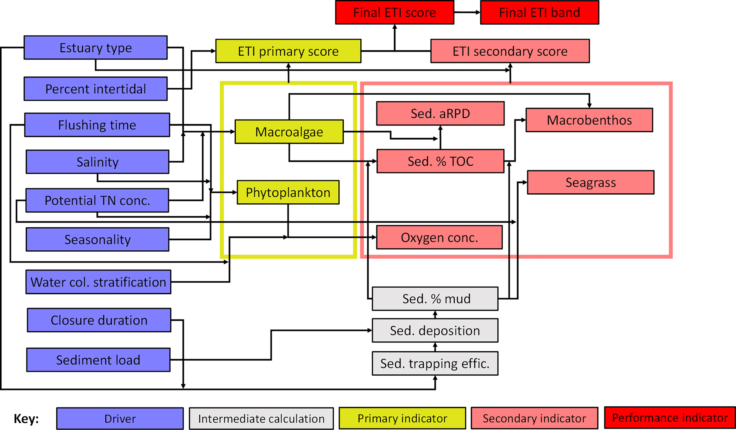
Figure 1 Schematic of the ETI Tool 3 BBN. Information on ‘drivers’ (blue nodes) are input by the user and the BBN calculates values of primary and secondary trophic indicators (yellow and pink ‘indicator’ nodes). Primary and secondary indicator values are used to produce ETI primary and secondary indicator scores, which are then combined to give the final ETI ‘performance’ score and band (red nodes). To simplify the schematic, yellow and pink rectangles indicate ‘standardisation nodes’ that normalise values of indicators prior to input to primary and secondary score nodes (see standardised indicator node section below).

Within the ETI Tool 3 BBN, most of the values of the drivers (Figure 1) are known in advance, from the outputs of ETI Tool 1. The values of indicators are calculated by the BBN model and combined to calculate the ETI score. ‘Intermediate calculation’ nodes are also included; these do not directly input to the scores but are used to calculate some of the indicators. Nearly all the relationships between these nodes are derived using observation or model – based information, rather than with a strong reliance on expert opinion. Although use of expert opinion is a recognised and valid method of informing BBN models (Uusitalo, 2007) we considered it preferable to rely, whenever possible, on observed or modelled relationships. Sections 2.2 and 2.3 summarise information underpinning the relationships, while detailed descriptions of the relationships, and the CPTs describing probability distributions of the responses of parent and child nodes, are given in the corresponding Supplementary Material (S.M.) sections. The nomenclature used in the study is provided at end of the article.

The ETI Tool 3 BBN combines the values of indicator nodes into a final ETI score of estuary health (its ‘performance node’, Figure 1). Indicators are distinguished as ‘primary’ or ‘secondary’ indicators. Primary indicators are potentially nuisance primary producers (i.e., macroalgae and phytoplankton) that commonly have demonstrably increasing responses to nutrient enrichment. Secondary indicators are ‘ecological symptoms’ of estuary health impairment (e.g., impaired macrobenthic health, high sediment carbon, reduced seagrass extent) arising as consequences of values of primary indicators and drivers. This distinction determines how primary and secondary indicator scores are combined into the final ETI score, where the score of the most impaired primary indicator is combined with the average of the secondary indicator scores (Robertson et al., 2016b). In NZ water quality policy statements (e.g., the NPSFM; New Zealand Government (2020)), freshwater water quality health variables are scored using a four-level banding (A-D). The ETI follows this protocol and the BBN uses four bands for most indicators and the overall ETI banding. The estuary health conditions associated with the bandings (A-D) of the ETI final score (adapted from Robertson et al. (2016b)) are described in Table 1.

TABLE 1

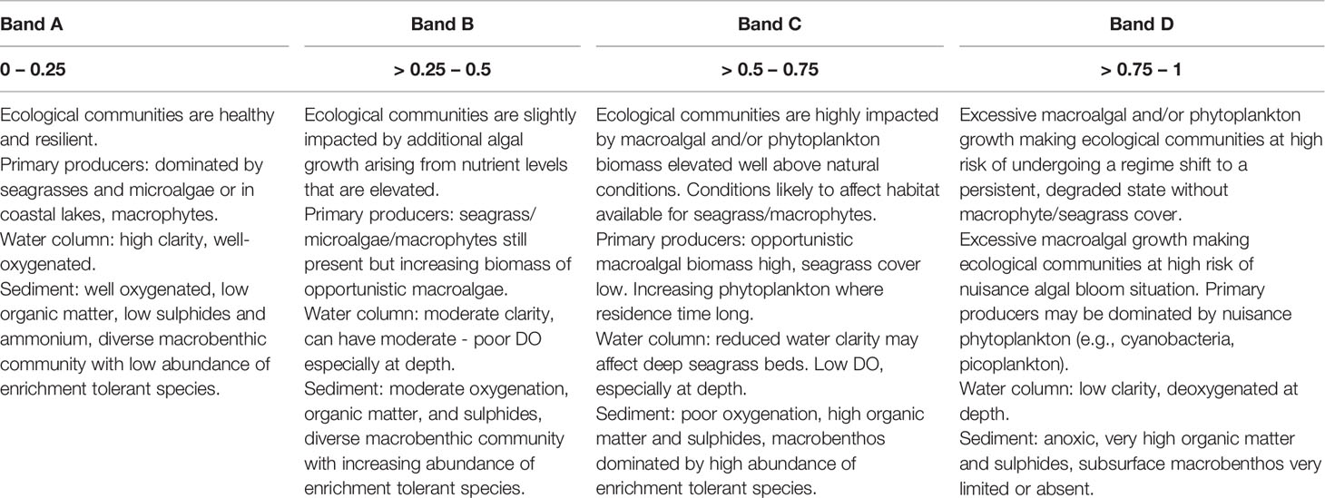
Table 1 Estuary health conditions associated with the bandings (A – D) of the ETI Tool 3 BBN final score (0 – 1) [adapted from Robertson et al. (2016b)].

2.2 Deriving Driver Nodes

The information for each driver node (indicated by bold text, below) in the ETI Tool 3 BBN (Figure 1) was derived from a combination of pre-existing physiographic information on NZ estuaries extracted from the NZ Coastal Explorer Database (Hume et al., 2007; Hume et al., 2016), updated with more recent survey data where available, and estuary dilution modelling based on that information (Plew et al., 2018). Methods used were those of Plew et al. (2020), where nutrient loads were either calculated from a GIS land use model (Elliott et al., 2016; Semadeni-Davies et al., 2020) updated using a land cover layer from 2017 to calculate nutrient loads, or from observed river flow and nutrient concentrations.

Estuary type was determined from the Coastal Explorer database of Hume et al. (2007) and Hume et al. (2016), or more recent surveys. This database also provided physiographic information necessary for the dilution modelling (Plew et al., 2018) used to estimate flushing time, salinity and potential total nitrogen (TN) concentrations (mg m^-3) in 291 tidal lagoons, tidal rivers and coastal lakes across NZ.

Potential TN concentrations are defined as those that would occur in the absence of uptake by algae, or losses or gains due to non-conservative processes such as denitrification (Plew et al., 2018). The ETI Tool 3 BBN assumes that nitrogen (N) is the limiting nutrient for macroalgal and phytoplankton growth and hence only uses potential TN and not phosphorus. Macroalgae have high N requirements compared to P (Atkinson and Smith, 1983), and macroalgal growth is more commonly limited by N rather than P in NZ estuaries (Barr, 2007; Robertson and Savage, 2018). For phytoplankton, Plew et al. (2020) predicted that 81% of the estuaries in the ETI Tool 1 dataset were limited by N. This latter result is mirrored by findings of dominant N limitation of estuarine phytoplankton in North American estuaries (NRC, 2000). The values of the potential TN driver node were more finely resolved at lower concentrations than at higher concentrations reflecting the need to distinguish TN at lower levels where macroalgal and phytoplankton growth change rapidly with concentration (Eppley et al., 1969; Barr, 2007; Dudley et al., 2022).

In the ETI Tool 3 BBN, the percent intertidal node and the ETI primary score node are linked (Figure 1) because the relative influence of phytoplankton and macroalgal eutrophication depends on estuary morphology (see below). The main effects of phytoplankton eutrophication are oxygen depletion and high light attenuation in deeper and often stratified estuarine systems. Such estuaries generally have little intertidal area suitable for nuisance macroalgae. In contrast, estuaries with large intertidal area as a percentage of total area are normally shallow and well mixed, and high phytoplankton concentrations are unlikely to result in low oxygen levels or significant light attenuation. However, estuaries with large intertidal areas are more suspectable to macroalgal blooms. The great majority of estuaries in the ETI Tool 1 database with intertidal areas less than 20% are tidal rivers, while the great majority of tidal lagoons have intertidal areas greater than 40% (Plew et al., 2020). The BBN selects the macroalgal primary indicator as the driver of the BBN primary score node for estuaries with intertidal areas greater than 40% to prevent the phytoplankton primary indicator having effect. For estuaries with intertidal areas less than 5% the BBN selects the phytoplankton primary indicator as the driver of the ETI primary score node. If the intertidal area is between 5% and 40%, the ETI primary score node is scored using the worst of the macroalgae and phytoplankton indicators.

The prevalence and ecological effects of phytoplankton blooms (particularly deoxygenation in the water column) usually are greater in summer when water column temperature and stratification are higher. It is therefore most appropriate to expose phytoplankton to potential TN concentrations that occur in summer. To capture this pattern, the Seasonality driver node is set as the ratio of potential TN calculated for summer to annual potential TN. Summer potential TN for each estuary was calculated using ratios of February (summer) to mean annual river flows and river nutrient concentrations (Booker and Woods, 2014; Whitehead et al., 2019). In most NZ estuaries, summer potential TN is lower than annual TN, giving seasonality factors less than 1. Flushing time is also calculated using mean February flows because it is used to predict phytoplankton biomass probabilities (Figure 1). If the user believes that the seasonality factor for an estuary was not appropriate (e.g., was set such that the importance of inputs during other seasons were undervalued), the seasonality factor can be set to a higher value.

Sediment load (g fine sediment m^-2 day^-1) were derived from a raster-based (gridded) empirical model that, for each 1 ha grid cell of NZ, relates the mean annual suspended sediment load to the average slope, mean annual rainfall, land cover, and lithology within that grid cell (Hicks et al., 2019). Sediment loads to each estuary were determined by summing the loads from grid cells within the catchment, and routing these loads down the stream network, considering entrapment in lakes and reservoirs. The sediment loading bands increase in size in an approximately exponential manner to encompass the wide range occurring in NZ estuaries (Hicks et al., 2019) while retaining sensitivity at the lower end of the range.

Driver nodes describing estuary closure duration and water column stratification are decided by the user, to examine scenarios involving those conditions. Additional information on these settings are given in relevant sections below.

2.3 Deriving Indicator Relationships and Conditional Probability Tables

Here we provide rationale for selection of each primary and secondary indicator in the ETI Tool 3 BBN, and then summarise the derivations of the CPTs linking them with their parent nodes (for additional detail, refer to corresponding sections of the Supplementary Material).

2.3.1 Macroalgae

High abundance of opportunistic macroalgae is a primary symptom of estuary eutrophication. Opportunistic macroalgae are highly effective at utilizing excess nitrogen, enabling them to out-compete other seaweed species. At nuisance levels, they can form mats on the estuary surface which adversely impact underlying sediments and other algae, macrobenthos, fish, birds, seagrass, and salt marsh (Valiela et al., 1997; NRC, 2000). Decaying macroalgae can accumulate sub-tidally and on shorelines causing oxygen depletion and nuisance odours. The greater the macroalgal cover, biomass, persistence, and extent of burial of algal material within sediments, the greater the subsequent impacts (Green et al., 2014; Sutula et al., 2014). In NZ, macroalgal biomass and spatial extent are key indicators of degraded ecological health in coastal lake, tidal lagoon and tidal river estuaries (Barr et al., 2013; Barr et al., 2020).

Plew et al. (2020) derived a relationship between potential TN concentrations and macroalgae Ecological Quality Rating (EQR) for 21 NZ estuaries. EQR is an estuarine macroalgal index that combines biomass and spatial measures, derived using the Opportunistic Macroalgal Blooming Tool (WFD-UKTAG, 2014), modified for NZ (Plew et al., 2020) and calculated for the whole estuary. To derive the macroalgae CPT (S.M. section 1), the resulting relationship along with the predictor uncertainty for the regression (Figure 2) predicted potential TN corresponding to EQR thresholds of 0.8, 0.6 and 0.4, which are the thresholds between A-B (minimal-moderate), B-C (moderate-high) and C-D (high-very high) bands of macroalgal eutrophication, respectively (Robertson et al., 2016b; Plew et al., 2020). We used annual TN loads and annual mean flows to calculate potential TN concentrations, while EQR observations were from peak growth (summer) periods. The bandings therefore relate annual loads and flows to summer macroalgal response.

FIGURE 2

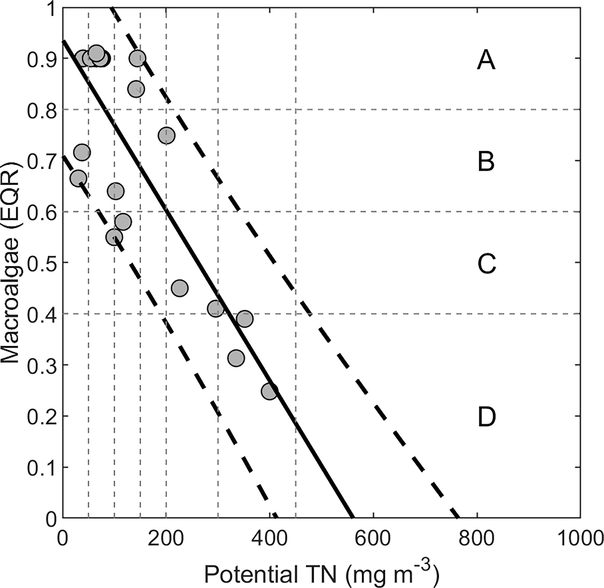
Figure 2 Observations of macroalgae Ecological Quality Rating (EQR) plotted against potential total nitrogen (TN) concentrations for 21 NZ estuaries. Data were from Robertson et al. (2016b); Plew et al. (2018) and Plew et al. (2020). Horizontal dotted lines demark thresholds between EQR bands (A–D) for macroalgae. Also shown are 95% prediction intervals (dashed lines) used for calculating proportion of observations in each EQR band at various potential TN levels (vertical lines).

We applied a high macroalgae EQR band (i.e., low biomass) if the estuary salinity (calculated from the dilution modelling) was less than 5 (practical salinity scale), because estuarine macroalgal growth is inhibited by low salinity (Martins et al., 1999; Dudley et al., 2022). This shifted the probability distributions for low salinity estuaries towards the A band, becoming increasingly in the B band with increasing potential TN. Tidal river estuaries, particularly those with high river flows and low intertidal area, often tolerate higher nutrient loads (in terms of expressing relatively little macroalgal eutrophication) than other estuary types (Robertson et al., 2016a). A combination of scour action, low salinities, and limited intertidal area tend to restrict macroalgal growth and accumulation in tidal river estuaries. The relationship between potential TN and EQR was developed using data mostly from tidal lagoons (Plew et al., 2020), and tidal river estuaries are poorly studied in comparison. Based on the few tidal river estuaries for which we have data, we estimated that potential TN thresholds for tidal rivers are ~ 3 × higher than for tidal lagoons and adjusted the macroalgae CPT for tidal rivers accordingly (Supplementary Table 1).

2.3.2 Phytoplankton

Prolific growth of phytoplankton are another primary symptom of eutrophication in estuaries (Bricker et al., 2003), which at nuisance levels can cause secondary symptoms including changes in water column and sediment chemistry, reductions in water clarity and dissolved oxygen, with impacts on macrophytes and higher trophic levels. High phytoplankton concentrations are responses to high nutrient loads (Woodland et al., 2015), and also estuary flushing time, being unlikely to occur in estuaries that have flushing times less than the phytoplankton doubling or turn-over times (Cloern, 1996; Ferreira et al., 2005).

The Phytoplankton CPT (S.M. section 2; Supplementary Table 2) was calculated from potential TN and flushing time (Figure 1) using the analytical model developed by Plew et al. (2020). This model predicts the highest likely phytoplankton concentration (as chl-a) expected under summer conditons. The model assumes a specific growth rate of 0.3 d^-1 (Plew et al., 2020) based on reported net growth rates for phytoplankton in NZ estuaries of <0.2 – 0.4 d^-1 (Vant and Budd, 1993; Gibbs and Vant, 1997). Flushing time values were chosen to range from those below which phytoplankton does not accumulate (< ~3 d) to those above which chlorophyll levels are determined solely by nutrient concentration (> ~10 d). Intermediate bands were chosen (3 to 6 d, and 6 to 10 d) to be spread between the minimum and maximum flushing rates. As described above (Driver Node section), the prevalence and ecological effects of high phytoplankton concentrations are greater in summer, so summer flushing times were used along with Potential TN concentrations, adjusted with the Seasonality driver node (Figure 1).

Different bandings were applied to phytoplankton concentrations based on salinity (Plew et al., 2020) (Supplementary Figure 2). This was accommodated using the Salinity driver node which modified Phytoplankton node values prior to their input to the ETI primary score node (Supplementary Table 3). For freshwater or brackish oligohaline (salinity < 5) systems, we applied bandings from the NPSFM for the maximum chl-a concentrations in lakes (New Zealand Government, 2020). Basque estuary thresholds (Borja et al., 2004; Robertson et al., 2016b) were used for banding mesohaline/polyhaline (salinity 5-30) systems and euhaline (salinity > 30) systems. The Basque estuary bandings and the NPSFM bands were developed for the 90th percentile of monthly observations (to indicate the highest observed phytoplankton concentrations). These bandings are applied to the predicted summer maximum chl-a concentrations from the model.

2.3.3 Mud

Estuary sediment deposition is a major factor impacting estuary conditions. High deposition of fine sediments leads to increased muddiness (expressed as % grain size less than 63 µm by weight), which can impair animal feeding, behavioural responses, larval recruitment, and trophic interactions in coastal food-webs (Lohrer et al., 2004; Lohrer et al., 2006; Jones et al., 2011; Pratt et al., 2014). Less permeable, muddy sediments often retain more nutrients (Huettel and Rusch, 2000; Engelsen et al., 2008), with associated elevated organic content and sulphides, low sediment oxygenation (i.e., shallow redox depth) and a depressed condition of sediment-associated invertebrate communities (Robertson et al., 2015; Robertson et al., 2017). NZ estuaries with less mud tend to be more favourable for healthy macrobenthic communities (Robertson et al., 2016c; Clark et al., 2019) and have been shown to be resilient to nutrient-driven eutrophication once the nutrient stressor is removed (Zeldis et al., 2020). There is often a positive feedback between fine sediment and nutrient loading and eutrophication, with muddy sediments and high nutrient loading favouring nutrient retention and macroalgal outgrowth (Robertson and Savage, 2018), with macroalgae in turn trapping more mud (Zeldis et al., 2019).

In the ETI Tool 3 BBN, muddiness interacts with other scored indicators but does not contribute directly to the ETI score. This is because eutrophic estuaries are not necessarily muddy, nor are muddy estuaries necessarily eutrophic. The mud node of the BBN was predicted from sediment deposition rates, which are in turn predicted using estuary type and sediment loads. Estuary mud deposition arises from fine sediment delivery (load) and trapping efficiency in the estuary (Figure 1). S.M. section 3 details the modelling of these processes by Hicks et al. (2019), used here. Estuary type is also a factor, with coastal lakes found to have highest trapping efficiencies, followed by tidal lagoons, with tidal rivers having lowest trapping efficiencies. Trapping efficiencies are further modified by estuary mouth closure duration.

To accommodate these factors, the modelled sediment deposition rate distributions were divided into seven bands from low to high (<0.1, 0.1-0.5, 0.5-1, 1-2, 2-5, 5-10, 10-20 mm y^-1), to derive the CPT linking trapping efficiency bands and load bands to deposition rate (Supplementary Table 7). Choice of these bands was informed by a default guideline value of 2 mm y^-1 of sediment accumulation above the natural annual sedimentation rate (Townsend and Lohrer, 2015). While natural sedimentation rates in NZ estuaries are not well known, the available information (Townsend and Lohrer, 2015) suggests that natural rates are generally considerably less than 1 mm y^-1. The deposition rate was then used to drive the Sediment % mud node (Figure 1) which is defined as the estuary - averaged value of % mud. Thresholds for estuary-averaged % mud of 12%, 25% and 34% were selected based on Robertson et al. (2016c) who showed these were important thresholds for macrobenthic health in NZ estuaries (see Macrobenthos node, below). We assumed that the default guideline value of 2 mm y^-1 above the natural annual sedimentation rate causes detrimental effects similar to those at 34% mud content, shown by Robertson et al. (2016c) to be associated with ‘transitional to pollution’ in terms of a locally calibrated macrobenthic health index (see Macrobenthos node, below). We thus equated a deposition of > 2 mm y^-1 with a % mud content of > 34% and, based on this approximation, the CPT linking fine sediment deposition rate to sediment % mud was created (Supplementary Table 8).

2.3.4 Sediment Total Organic Carbon

Estuarine sediments with high percent total organic carbon (% TOC) are often associated with chronic macroalgal blooms which, upon decomposition, contribute locally produced (autochthonous) organic matter to sediments (Sutula et al., 2014). The rate of autochthonous organic matter production and its microbial respiration are thus key elements of the estuarine eutrophication problem, associated with adverse sedimentary environmental conditions including depleted oxygen and excessive ammonium and hydrogen sulphide concentrations (Gray et al., 2002; Hyland et al., 2005). High % TOC is also commonly associated with muddy sediments (Pelletier et al., 2011), which are less likely to be well irrigated compared to more permeable, sandy sediments (Huettel and Rusch, 2000; Engelsen et al., 2008; Zeldis et al., 2020). Furthermore, allochthonous mud has significant organic matter content in NZ rivers (Scott et al., 2004; Zeldis et al., 2010). We therefore developed the Sediment % TOC node to react to an interaction of the Macroalgae and Sediment % mud nodes in the ETI Tool 3 BBN.

Relationships between macroalgal biomass and sediment % TOC of Sutula et al. (2014) were used to derive a CPT estimating effects of macroalgal accumulation on % TOC (S.M. Section 4, Supplementary Table 9). We determined a four-band gradient of % TOC from low to high impact by considering % TOC effects on sediment apparent Redox Potential Discontinuity (aRPD) (Sutula et al., 2014) and macrobenthic condition (Robertson et al., 2016c).

We used sediment % mud and sediment % TOC data from five Southland (NZ) estuaries (New River, Jacobs River, Haldane, Fortrose and Freshwater Estuaries (Robertson et al., 2017) (L. Stevens, Salt Ecology Consultants, NZ, pers. comm) to derive a CPT relating sediment % mud to sediment % TOC (Supplementary Table 10; Supplementary Figure 4).

The final macroalgae/sediment % mud/sediment % TOC CPT (Supplementary Table 11) was derived by cross-multiplying and normalising Supplementary Tables 9, 10.

2.3.5 Apparent Redox Potential Discontinuity Depth

The apparent Redox Potential Discontinuity (aRPD) depth marks the depth of the boundary between oxic near-surface sediment and the underlying suboxic or anoxic sediment. Shallowing of aRPD is related to reduced benthic habitat quality and volume, deleterious alterations in macrobenthic community structure (Green et al., 2014) and undesirable changes in sedimentary biogeochemical cycling (Eyre and Ferguson, 2009; Sutula, 2011). Shallow aRPD is often associated with excessive organic matter additions from macroalgae (Macroalgal EQR section, above; Sutula et al. (2014)), in estuary types that support appropriate conditions for macroalgal blooms (most commonly tidal lagoons in NZ). As described above (Sediment TOC section), excessive TOC associated with muddiness can lead to depleted oxygen, and excessive ammonium and hydrogen sulphide concentrations in sediments.

The aRPD CPT therefore considers the interacting effects of macroalgal eutrophication and % TOC bands on aRPD (Figure 1) (S.M. section 5). A regression between sediment % TOC and aRPD was derived using Sutula et al. (2014) and combined with a regression between macroalgal EQR and % TOC using Sutula et al. (2014) and Green et al. (2014). This resulted in bands of aRPD ranging from a low impact ‘reference threshold’ of > 4 cm to an ‘exhaustion threshold’ of < 1 cm, with intermediate thresholds at 2.5 to 4 cm and 1 to 2.5 cm conditioned by the 4 bands of EQR and % TOC. The probability of aRPD falling in each of the four aRPD bands was then calculated for each of the 16 combinations of % TOC and EQR bands (Supplementary Table 13).

2.3.6 Macrobenthos

Excessive macroalgal biomass, high % TOC in sediments, and excessive muddiness can act synergistically to affect the health of macrobenthos, by smothering their habitats and by creating anoxic and sulphidic conditions in their sedimentary environments (Green et al., 2014; Pratt et al., 2014; Robertson et al., 2015; Robertson et al., 2016c). The macrobenthic CPT was therefore constructed to incorporate interacting effects of macroalgal biomass, % TOC and muddiness.

Robertson et al. (2016c) developed regression trees that identified threshold values of % mud and % TOC delimiting macrobenthic taxon abundance and richness at 21 NZ tidal lagoon and tidal river estuaries. These were expressed in terms of AMBI (AZTI Marine Benthic Index) (Borja et al., 2000) Biotic Coefficients, which ranged from ‘Normal’ (1.2 – 3.3) to ‘Transitional to pollution’ (3.3 – 4.3), to ‘Polluted’ (> 4.3), with increasing % mud. % TOC values were only important as a criterion for abundance and richness indices if % mud was very high (> ~34% for abundance-weighted AMBI), indicating organic enrichment rather than muddiness was the primary stressor for that split. Robertson et al. (2016c) concluded that the locally (NZ) calibrated AMBI (‘NZ AMBI’) provided a robust proxy of stress, relating % mud and % TOC to macrobenthic community health.

Green et al. (2014) described macroalgal eutrophication effects on macrobenthic health, indicating that macroalgal biomasses below 15 g dm (dry mass) m^-2 had no negative effects on macrobenthos, while a value of 110 g dm m^-2 was an approximate midpoint between ‘no effect’ and an ‘exhaustion threshold’ occurring at ~185 g dm m^-2. The latter value corresponded well with the value of 175 g dm m^-2 found by Sutula et al. (2014) for an exhaustion threshold for aRPD. These values were converted to EQR equivalents (S.M. section 5).

The macroalgal EQR, % mud and % TOC thresholds were combined to derive the macrobenthic CPT, in terms of NZ AMBI Biotic Coefficients (S.M. section 6, Supplementary Table 14). We set % TOC to have increasing influence only after % mud exceeded 34% and after macroalgal EQR was < 0.4. Macroalgal biomass had no influence at high EQR (≥ 0.8) and had increasing influence at EQR < 0.8, where it corresponded to values exceeding reference conditions of Green et al. (2014).

2.3.7 Oxygen

Oxygen is essential for aquatic ecosystems because it enables organisms to extract energy from organic matter (Lehninger, 1975). When respiratory consumption of estuarine water column oxygen becomes greater than replenishment by photosynthesis or hydrodynamic and atmospheric exchange, oxygen concentrations are decreased and can become stressful for biota (hypoxia) (Gray et al., 2002; Vaquer-Sunyer and Duarte, 2008). In extreme cases, hypoxia can be catastrophic for biota and normal biogeochemical functioning of coastal ecosystems (Conley et al., 2009).

Estuarine water column hypoxia can arise from seasonal decomposition of organic matter by microbial respiration (Wallace et al., 2014; Zeldis and Swaney, 2018; Zeldis et al., 2022), meaning that the extent of oxygen depletion can be a positive function of nutrient inputs and phytoplankton biomass during the production season (NRC, 2000; Harding et al., 2014; Wallace et al., 2014). For regulatory purposes, achievement of desired levels of water column oxygen have therefore been tied to limits of phytoplankton biomass (often measured as chl-a; e.g., Harding et al. (2014)). Physical processes also affect estuary hypoxic susceptibility (Scully, 2016) if the water column becomes density-stratified, acting to isolate the deeper layers from atmospheric exchange. If the water column is shallow or regularly vertically mixed, atmospheric exchange is maintained and hypoxic conditions generally will not form. Residence time also governs oxygen levels, with longer flushing times more likely to sustain low oxygen waters. Observations in NZ have shown that shallow tidal lagoons and tidal rivers with short residence times are normally well mixed and are unlikely to exhibit low water column-average oxygen concentrations (Dudley et al., 2017). Some tidal rivers may, however, include deep areas which support saline stratification, and coastal lakes are non-tidal so may be more susceptible to stratification and low oxygen.

The water column oxygen CPT in the ETI Tool 3 BBN was therefore driven by interactions of phytoplankton biomass, flushing and stratification (Figure 1; S.M. section 7). Its bandings (Supplementary Table 15) were set using the 7 day mean minimum thresholds given in Robertson et al. (2016b) (their Table 7), which were based on NZ National Objective Framework (NOF) criteria for rivers (Davies-Colley et al., 2013) and California estuary criteria (Sutula et al., 2012). These thresholds identified oxygen levels ranging from no stress/minor stress on aquatic organisms at oxygen levels ≥ 7 mg L^-1, to significant, persistent stress with likelihood of local extinctions and loss of ecological integrity at < 5.0 mg L^-1.

Because we were unable to predict the stratification strength of estuaries in the ETI Tool 3 BBN, it was included as a user-input driver (Figure 1; Supplementary Table 16) that prescribes whether estuaries are stratified or not. The linkages of stratification, flushing and phytoplankton nodes were determined using field-derived oxygen utilisation rates, chl-a and physical data from Firth of Thames, a NZ North Island estuary (Zeldis et al., 2022). These yielded a chl-a - specific rate of oxygen drawdown (detailed in S.M. section 7) for both stratified and non-stratified states in the estuaries.

2.3.8 Seagrass

Seagrass (Zostera muelleri) is a vascular, rooted estuarine macrophyte that is a keystone ecological component of many NZ estuaries (Robertson et al., 2016b). Seagrass provides high value habitat for a wide range of biota in NZ (Morrison et al., 2009) and important ecosystem services including wave attenuation, increased water clarity, denitrification and carbon sequestration (Reynolds et al., 2016; Duarte and Krause-Jensen, 2018). The presence of seagrass beds in good condition is generally considered to indicate low/moderate nutrient and mud inputs and good water quality, while large scale seagrass losses have been documented where these conditions have not been met (Inglis, 2003; Morrison et al., 2009).

Increased N loads have been associated with 80% to 94% reductions in dense seagrass in southern South Island NZ estuaries (Zeldis et al. (2019); reviewed in S.M section 8), often associated with excessive macroalgal cover and muddiness. Recent work in Porirua Harbour (southern North Island, NZ) (Zabarte-Maeztu et al., 2019) has found a threshold of 23% mud, above which NZ seagrass does not occur. Nutrient toxicity effects on seagrass are also important at high concentrations (~25 µmol L^-1 ${\text{NH}}_4^{+}$ -N; Katwijk et al. (1997) and 6-12 µmol L^-1 ${\text{NO}}_3^{-}$ N; Burkholder et al. (1994)).

Considering this information, the seagrass CPT (S.M. section 8; Supplementary Table 18) in the ETI Tool 3 BBN was constructed assuming that potential TN concentration and % mud are key drivers of seagrass condition (Figure 1). We considered that potential TN ≥ 150-200 mg m^-3 (~10 – 14 µmol L^-1) were likely to elicit macroalgal growths at the B/C EQR band threshold (Macroalgal EQR section, above), that would correspond to poor conditions for seagrass arising from both eutrophication and nitrate and/or ammonium toxicity. Further, we assumed that % mud ≥ 25-34% would elicit deleterious effects. The metric employed for assessing seagrass health was extent of seagrass cover as percentage of estimated natural state cover (ENSC: Robertson et al. (2016b)), with values from 95% to 85% ENSC signifying moderate stress (C band) and < 85% significant, persistent stress (D band).

2.3.9 Standardised Indicators

The full ETI Tool 3 BBN NETICA structure (Figure 3) includes the distribution of values for each primary and secondary node and their means and standard deviations. The values in each primary and secondary node were expressed in their original units and over various ranges (Figure 3). To linearise and normalise these values prior to input to the primary and secondary scoring nodes, ‘standardised nodes’ are used to convert the values to a range of zero to one, using four equal-sized bands (Figure 3).

FIGURE 3

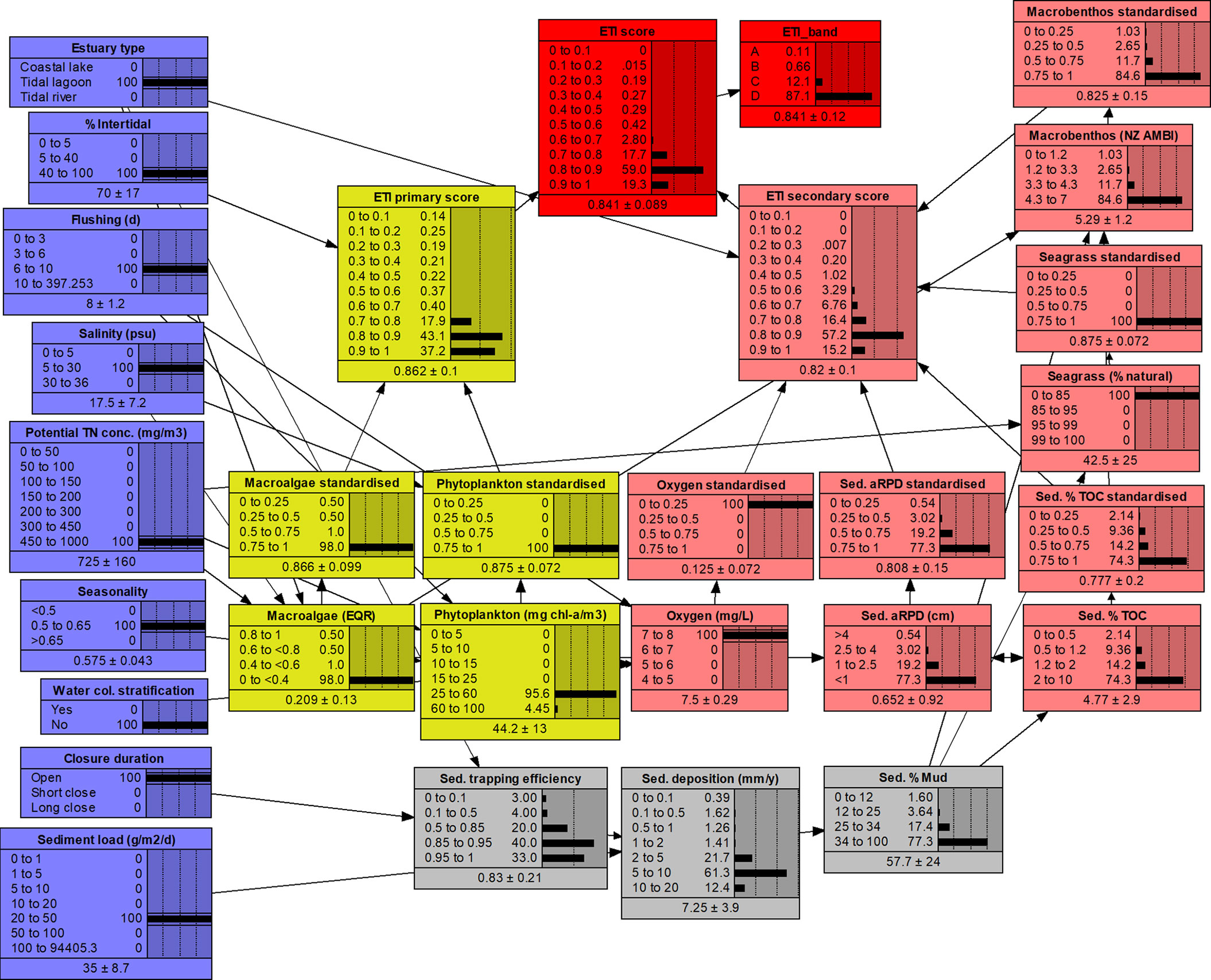
Figure 3 ETI Tool 3 BBN NETICA structure. Blue boxes are driver nodes with values input from ETI Tool 1, yellow and pink nodes are primary and secondary indicator nodes and the red nodes are the final ETI score and bands. Grey nodes are intermediate calculation nodes. Indicator nodes have accompanying standardising nodes that normalise their respective scores prior to input to the primary and secondary scoring nodes. This BBN run shows results for Jacob River Estuary (Southland region, NZ) in its present state.

2.3.10 ETI Primary Score

The ETI primary score CPT is calculated from the standardised primary indicator values for macroalgae and phytoplankton. The ETI primary score is discretised into 10 bands to improve precision of the estimate as it combines multiple indicators. The calculation uses an equation that includes the percent intertidal area driver node (Figure 1), to determine which of the two primary indicators (macroalgae or phytoplankton) to use in the primary indicator scoring (Driver Nodes section, above). If intertidal area is < 5%, phytoplankton is selected, if > 40% macroalgae is selected and if between 5 and 40% the larger of the two is selected.

$$ET{I}_{pri}=\{\begin{array}{cc}Phyt{o}_{std}& Intertidal<5\%\\ max\left(Phyt{o}_{std},Macr{o}_{std}\right)& 5\le Intertidal\le 40\%\\ Macr{o}_{std}& Intertidal>40\%\end{array}$$

The ETI primary score node table which incorporates these settings and maps them to the various combinations of standardised macroalgae and phytoplankton scores is very large and is not shown in Supplementary Material. However, it may be examined by opening that node using the ETI Tool 3 BBN application and opening the ‘Table’ tab. This is also true for the ETI secondary score CPT, and the ETI final score CPT, described below.

2.3.11 ETI Secondary Score

The ETI secondary score CPT is calculated using an equation that selects the average of standardised secondary indicator node scores using the equation:

$$ET{I}_{sec}=average\left(aRP{D}_{std},Macrobentho{s}_{std},TO{C}_{std},Seagras{s}_{std},Oxyge{n}_{std}\right)$$

Like the primary score, the secondary score is discretised into 10 bands. For shallow, well mixed tidal lagoon estuaries, where significant water column oxygen depletion is typically absent, the ETI secondary score is calculated without the oxygen term.

2.3.12 ETI Score and ETI Band

The ETI score CPT is calculated using an equation that selects the average of the primary and secondary scores, using the equation:

$$ETI=\left(ET{I}_{pri}+ET{I}_{sec}\right)/2$$

The ETI score is discretised into 10 bands. As an additional step, the ETI score could be recast as four bands (A-D) if it were needed to make comparison with the 4-state banding used within the NPSFM. This is the ETI band shown in Figures 1, 3. In this study, we use the ETI score calculated from the 10 banded node when comparing with ETI Tool 1 (Plew et al., 2020) and ETI Tool 2 scores (Zeldis et al., 2017b).

2.4 Comparisons With Estuary Observations

The ETI Tool 3 BBN was tested against observations from 11 NZ estuaries. The 11 estuaries and their associated Driver node inputs to the BBN, obtained by running ETI Tool 1, are described in Table 2. Observations of estuary eutrophication indicators were collected in a manner that allowed an ETI score to be calculated following the ETI Tool 2 protocol described by Robertson et al. (2016b) and available via https://shiny.niwa.co.nz/Estuaries-Screening-Tool-2/. Indicators measured in each estuary included macroalgal EQR, sediment redox potential (SRP) at 1 cm depth, sediment total organic carbon, sediment total nitrogen, NZ AMBI and area-weighted estuary mud content. These data were extracted from monitoring reports prepared for NZ regional councils (Table 3). Note that it was not necessary to have measurements for all secondary indicators to calculate an ETI Tool 2 score for an individual estuary.

TABLE 2

Table 2 Properties of 11 New Zealand (NZ) estuaries, used as Driver node input values to test the ETI Tool 3 BBN.

TABLE 3

Table 3 Observed estuary health indicator values from 11 NZ estuaries and resulting ETI Tool 2 score.

The ETI Tool 3 BBN uses aRPD, whereas the measured indicator in monitoring reports was SRP. In comparing ETI Tool 3 BBN predicted scores and ETI Tool 2 observed scores, we assumed that these metrics measure similar characteristics of sediment health, as also found by Gerwing et al. (2018).

In many of the monitoring reports the “percent of estuary area with > 25% mud content (< 63µm)” was used as a secondary indicator, contributing directly to the observed ETI Tool 2 score. In the ETI Tool 3 BBN, % mud does not contribute directly to the ETI score but influences other secondary indicators that do (Figures 1, 3). To be consistent with the BBN scoring, observed mud content was not included when calculating the observed ETI Tool 2 score (Table 3). The BBN uses estuary – average % mud, rather than “percent of estuary area with > 25% mud content (< 63µm)”. To make the observed (ETI Tool 2) mud metric comparable to the predicted (BBN) metric prior to its input to the BBN, we estimated area-weighted, average % mud content for each estuary using the mapping of sediment types and % mud content of each sediment type provided in the monitoring reports.

Dissolved oxygen, phytoplankton and sea grass cover were seldom measured in the observations, so for consistency these were excluded from the ETI Tool 3 BBN scores.

ETI Tool 2 scores calculated from the observations were first compared to ETI Tool 3 BBN scores using only Driver node data obtained from ETI Tool 1. We also compared observed and predicted indicator values, individually. Finally, observed values of indicators were used to set their respective nodes in the BBN, to determine which observations provided the most benefit in refining BBN predictions of ETI score.

2.5 Comparison With ETI Tool 1 Susceptibility

Predicted primary scores and ETI Tool 3 BBN scores were compared with susceptibility values from ETI Tool 1 (Plew et al., 2020). While ETI Tool 1 gives susceptibility as a band (A-D), the calculations for macroalgae and phytoplankton susceptibility each produce a continuous value for either EQR or chl-a. Those values were normalised between 0 and 1 using their respective band thresholds and used to predict a continuous susceptibility score, equivalent to the ETI primary score in the BBN. This susceptibility score was then compared to the BBN primary score and overall ETI score. In this analysis we assumed that tidal lagoons were not stratified. Stratification conditions in coastal lakes and tidal rivers were not simple to predict, therefore we did not set the stratification driver node in the BBN in those cases. By not setting the stratification driver node, an equal probability of the estuary being stratified or not was ascribed. For comparison with ETI Tool 1 susceptibility scores we included oxygen and seagrass indicators in the predicted ETI score.

3 Results

3.1 Correspondence With Observed ETI Tool 2 Scores

Comparisons of ETI Tool 3 BBN predicted scores with ETI Tool 2 observed scores for the 11 estuaries are given in Figure 4. When the BBN was driven only with inputs generated by ETI Tool 1, the predicted ETI scores were generally consistent with observed scores, with a root-mean-squared-error (rmse) of 0.121 (Figure 4A). Error bars on these estimates show the standard deviation of prediction based on the probability distributions of child nodes calculated by the BBN. Predicted scores for two of the estuaries (Whanganui Estuary and New River Estuary) lie more than one standard deviation below the 1:1 line. Standard deviations of the predicted scores were between 0.089 and 0.159 (averaging 0.129).

FIGURE 4

Figure 4 Comparison of ETI Tool 2 scores from observations and scores predicted by the ETI Tool 3 BBN using (A) only driver node data (predicted by ETI Tool 1), and with the addition of observed (B) macroalgal EQR, (C) sediment % TOC, (D) NZ AMBI, (E) average % mud content, and (F) EQR + % TOC + % mud + NZ AMBI. Shown are the root mean squared error (rmse) and error bars showing the standard deviation of the predicted BBN score. Estuaries were not shown in (C–E) when their additional secondary indicator observations were not available.

Observed macroalgae EQR values were available for all 11 estuaries. When observed EQR scores were included as an input to the ETI Tool 3 BBN (Figures 4B, F), the standard deviation of each prediction reduced to between 0.075 and 0.099 (average 0.086). This reflected the strong influence that the macroalgae EQR node had on secondary indicator nodes in the BBN. While the rmse reduced to 0.092, more (five) of the predicted ETI scores were more than one standard deviation below the 1:1 line. This was particularly the case for tidal river estuaries (red symbols in Figure 4B) with two of the three tidal river estuaries more than one standard deviation below the observed ETI Tool 2 score. The BBN predicted score was also substantially reduced in the Catlins Estuary where the addition of EQR reduced the predicted score from 0.609 to 0.445. These estuaries were systems where high macroalgae EQR was observed relative to nutrient loading.

% TOC observations were available for nine of the 11 estuaries. If % TOC was provided along with ETI Tool 1 inputs, rmse increased from the default scenario to 0.131, but the standard deviation of each prediction reduced to between 0.066 and 0.132 with a mean of 0.102 (Figure 4C).

Using observed NZ AMBI (available for nine estuaries) as an input to the ETI Tool 3 BBN resulted in the highest rmse of 0.160 (Figure 4D), although the standard deviation of each prediction reduced to between 0.068 and 0.130 (average 0.101). Much of the increased rmse was caused by the higher predicted ETI score for Shag River Estuary, with predicted ETI scores for other estuaries changed by only small amounts.

% mud content is not scored as a secondary indicator in the ETI Tool 3 BBN, but directly influences secondary indicators of % TOC and NZ AMBI (as well as seagrass which is not scored in this comparison). Percent mud content calculated as an area weighted average was estimated for eight of the estuaries. Adding % mud to the BBN resulted in the lowest rmse of 0.087, although predicted ETI scores were biased low compared to observations (Figure 4E). Standard deviations of each prediction were between 0.088 and 0.159 (average 0.125).

When all the available observations of indicators were used as inputs to the ETI Tool 3 BBN (Figure 4F), the rmse was 0.098. The standard deviations for each prediction were in the range 0.063 to 0.081 (average 0.070). Predicted BBN scores were within one standard deviation of ETI Tool 2 observed scores for six of the 11 estuaries, and within two standard deviations for another three estuaries. The exceptions were the Catlins Estuary and Toetoes Estuary. The BBN score for Toetoes Estuary was underpredicted mostly because the estuary has low % mud and EQR (the only two observed indicators available as inputs for the BBN) due to strong currents over large portions of the estuary that scour macroalgae and restrict mud accumulation (Stevens, 2018a). Poor sediment oxygenation has been reported over large areas of the estuary (Stevens and Robertson, 2017c; Stevens, 2018a), and a low SRP at 1 cm depth (-400 mV) is included in the input to the observed score. Adding an aRPD score of < 1 cm to the BBN increases the predicted ETI score from 0.54 ± 0.07 to 0.59 ± 0.07, closer to, but still lower than, the observed value of 0.84.

For the Catlins Estuary, adding observed macroalgae EQR, % mud and % TOC all reduced the ETI Tool 3 BBN score. The observed ETI Tool 2 score included sediment SRP at 1 cm depth (-241 mV), which indicates anoxic conditions. Observations report widespread areas with low aRPD (Stevens and Robertson, 2017a) and including an aRPD of < 1 cm as input to the BBN raised the predicted ETI score from 0.44 ± 0.07 to 0.52 ± 0.06, closer to the ETI Tool 2 observed value (0.62). Another contributing factor to the low predicted BBN values is that the macroalgae EQR value of 0.62 is just above the lower end of the 0.6 to 0.8 band. If the observed EQR were slightly lower (in the 0.4 to 0.6 EQR band) then the BBN score would increase to 0.65 ± 0.07. This reflects one disadvantage of using only four bands for indicator nodes as, while having few bands is preferable to keep the CPTs manageable, small changes in observed indicator values that cross band thresholds can have large impacts on BBN scores. The observed ETI Tool 2 score uses a 10-level discretisation for indicators, which reduces this effect.

3.2 Comparing Predicted and Observed Indicator Values

Predictions of indicator values from the ETI Tool 3 BBN, supplied with only driver node inputs, were compared with indicator values derived from estuary observations (Figure 5). Predicted macroalgae EQR and NZ AMBI values (Figures 5A, E) were positively and significantly (p < 0.01) correlated with observations. Predicted aRPD and observed SRP at 1 cm depth were also positively and significantly (p < 0.05) correlated (Figure 5C) as were predicted and observed % TOC (Figure 5D). Observed and predicted % mud were not correlated (Figure 5B).

FIGURE 5

Figure 5 Comparison of observed estuary eutrophication indicator values with values predicted by the ETI Tool 3 BBN for (A) macroalgal EQR, (B) average % mud, (C) SRP at 1 cm depth and aRPD depth, (D) % TOC, and (E) NZ AMBI.

For the analyses of Figures 4, 5, errors were not available for observed ETI Tool 2 score or for individual indicators, respectively. This stems from the fact that multiple observations were available only for some of the observed indicators, in some of the estuaries, in original data reports.

3.3 National Scale ETI Tool 3 BBN Results and Correspondence With ETI Tool 1 Susceptibility

At the national scale, ETI Tool 1 susceptibility (Figure 6A) and ETI Tool 3 BBN score (Figure 6B) showed broadly corresponding patterns. The west coast of South Island had both lower susceptibility and BBN score than on the east coast. On the southeast South Island coast, susceptibility scores were higher (worse) than those from the BBN. In the North Island, correspondence between the two ETI tools was more variable. On the southeast coast of the North Island, ETI Tool 1 predictions tended to be lower than those of the BBN. For the North Island generally, regional patterns were less evident for both tools.

FIGURE 6

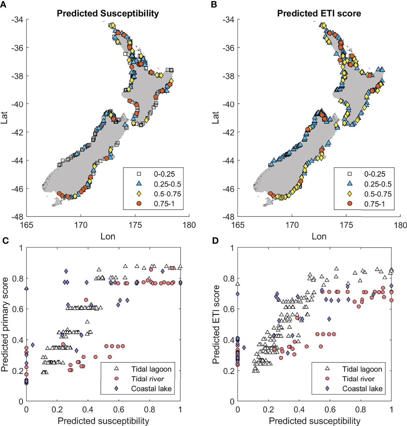
Figure 6 (A) Predicted eutrophication susceptibility from ETI Tool 1 (Plew et al., 2020), (B) Predicted ETI Tool 3 BBN score, (C) Comparison of ETI Tool 1 susceptibilities and BBN-predicted primary scores, and (D) ETI Tool 1 susceptibilities and BBN-predicted ETI scores.

Compared to ETI Tool 1 susceptibility scores (Figure 6A), the ETI Tool 3 BBN-predicted scores (Figure 6B) were compressed with fewer values in the ranges 0-0.25 (A band), and 0.75-1 (D band) (cf. Table 1). Many of the low susceptibility scores occur in tidal river estuaries which have both low salinity (which inhibited macroalgal growth), and short flushing times (which did not support phytoplankton blooms). These estuaries have a zero-susceptibility score (Figures 6C, D). With the BBN, these estuaries receive non-zero values (Figures 6C, D), which commonly map to the A or B band.

4 Discussion

4.1 Performance of the ETI Tool 3 BBN

The ETI scores predicted by the ETI Tool 3 BBN, using only driver node data obtained from ETI Tool 1, showed good agreement with ETI Tool 2 scores calculated from observations (Figure 4A). Figure 4 suggests that the ETI scores of tidal lagoons and tidal rivers are predicted with similar accuracy; however, the validation dataset is small (11 systems), particularly for tidal rivers (3 systems). Our validation dataset did not include any coastal lakes thus we cannot assess the accuracy of the BBN for those systems.

Adding all observed indicator values (Figure 4F) improved the agreement between predicted and observed ETI scores, although addition of individual indicators did not always do so. Adding % mud or macroalgae EQR indicators improved the fit, while adding % TOC or NZ AMBI did not. Correlations between individual predicted and observed indicators were not as strong (Figure 5). Within an individual estuary, the values of indicators can be highly variable in space and time and can indicate disparate levels of trophic condition amongst themselves (Green et al., 2014; Sutula et al., 2014). It is therefore beneficial to use multiple indicators to assess estuary health, as achieved by the overall ETI Tool 3 BBN score. The correlations between observed and predicted indicator values were also affected by the discretisation of most of the indicators within the BBN into four relatively broad bands over their respective ranges (Figure 3). Mean values were calculated from the midpoints of each band weighted by the probability predicted for each band by the BBN. Confidence intervals were calculated in a similar manner. The consequence of this is that confidence intervals were wide (Figure 5) due, in part, to the discretised structure of BBNs, generally. Furthermore, there was uncertainty in the observations, which was often unspecified in original data reports (often only one value was provided in the underlying reports). Uncertainties in those values would contribute to the overall errors between predicted and observed values of indicators. Also, we lacked data to test the BBN predictions for dissolved oxygen, seagrass and phytoplankton. Plew et al. (2020) compared the phytoplankton model to observations but found that available data seldom provided an unbiased estimate of volume-averaged chl-a concentrations and were of limited use for calibrating or validating the model.

ETI Tool 3 BBN-predicted values of % mud were the most poorly correlated with observations (Figure 5B). Percent mud is difficult to predict because the processes by which fine sediments are transported to and through estuaries, and how they settle, consolidate, or are resuspended by currents or waves, are complex. These can, at best, only be approximated using simple basin-averaged models such as used here (Hicks et al., 2019). Deposition is spatially and temporally variable and influenced by particle size, density, and flocculation processes, adding variability among observations. The BBN also relied on an assumed relationship between sediment accumulation rate and muddiness of 2 mm y^-1 ≈ 34% mud content which was poorly constrained. Consequently, our ability to predict % mud from annual fine sediment load is currently poor. While we did not use % mud as a scored secondary indicator when calculating the ETI secondary score, it has at times been used as an indicator in ETI Tool 2 scores (Robertson et al., 2016b). To compare our predicted % mud metric with observations (Figure 5B), we converted the ‘area of estuary with > 25% mud content’ of Robertson et al. (2016b) to ‘estuary averaged % mud content’. Our conversion between these metrics probably introduced further error.

The ETI Tool 3 BBN provides an overall score that represents the whole of an estuary, which is the same approach as that of ETI Tool 2. This is useful for management purposes for screening and scenario testing at the estuary-wide scale. While it doesn’t explicitly resolve within-estuary spatial or seasonal behaviours, it does use some indicators that use spatially-distributed sampling to measure a whole estuary response, for example EQR (WFD-UKTAG, 2014), or measure worst-case seasonal scenarios, for example chl-a (90^th percentile of observations: Plew et al. (2020)). We therefore regard the BBN characterizations as having reasonable skill in describing estuarine trophic conditions and likely responses to changes in forcing (e.g., nutrient loadings) at the estuary-wide, annual scale, while acknowledging that spatially localised or temporal responses may be inaccurately characterized.

Comparison of ETI Tool 1 susceptibility scores with ETI Tool 3 BBN primary scores showed ‘stepping’ (Figure 6C) due to the way the primary indicators (macroalgae EQR and phytoplankton) were discretised and combined within the BBN to obtain the primary indicator scores. ETI scores from the BBN showed less stepping, due to the averaging effect of inclusion of secondary indicators (Figure 6D).

Three other features were apparent when comparing the ETI Tool 3 BBN scores to ETI Tool 1 susceptibility scores. Firstly, as noted in Results, there were several estuaries (particularly tidal river estuaries and coastal lakes) where ETI Tool 1 predicted a zero susceptibility, because they may have either low salinity or low intertidal area, and therefore no macroalgae, or a short flushing time, so therefore no phytoplankton blooms. The BBN provided a non-zero predicted ETI score in these cases, due to both the inclusion of secondary indicators and because the probability distributions within the BBN’s CPTs allowed for non-zero outcomes. Secondly, a different relationship was seen between ETI Tool 1 and the BBN for tidal river estuaries than other estuary types (Figures 6C, D). This arose because ETI Tool 1 did not treat the estuary types differently, unlike the BBN, where the macroalgal response and sediment trapping efficiency were conditioned by estuary type. Finally, the distribution of ETI scores predicted by the BBN, and to a lesser extent predicted primary indicator scores, were compressed at the upper and lower limits, with maximum and minimum values of ~0.9 and 0.2. This is an artifact of the probability distributions built into BBN CPTs, which can spread predictions for indicators, and their resulting scores, over several bands (Uusitalo, 2007). Mean values for each indicator and the ETI score were calculated from those probability distributions (using the centre of each band weighted by the probability distribution across each band), tending to bring the ETI scores away from the limits of 0 or 1. Adding observed values of indicators (in particular EQR; Figure 4) would likely reduce the uncertainties within the BBN and could extend the range of its ETI scores toward the limits.

4.2 Applying the ETI Tool 3 BBN to Inform Estuary Management

We illustrate how the ETI Tool 3 BBN can be used to test or develop management strategies with two case study examples. First, we show how the BBN can be used to evaluate the efficacy (in terms of estuary health improvement) of wastewater diversion from an urban estuary via construction of an ocean outfall. The Avon-Heathcote Estuary (AHE) at Christchurch, South Island, is a small (7 km²) tidal lagoon estuary that received all of Christchurch’s (present population 330,000) wastewater, until the commissioning of a $NZ 80 M ocean outfall in March 2010 diverted its tertiary-treated wastewater offshore to the adjacent ocean (Zeldis et al., 2020). Prior to the diversion, the wastewater (ca. 170,000 m³ d⁻¹ in 2005) contributed ca. 88% of the AHE’s ${\text{NH}}_4^{+}$ -N load at 5500 kg d⁻¹ (Bolton-Ritchie and Main, 2005), resulting in heavy macroalgal eutrophication (Barr et al., 2020). In contrast, most of its ${\text{NO}}_3^{-}$ N load (ca. 94%, 470 kg d⁻¹) came from the Avon and Heathcote Rivers and municipal drains (Burge, 2007).

Monitoring data (Barr et al., 2020; Zeldis et al., 2020) showed that the wastewater diversion resulted in a dissolved inorganic nitrogen load reduction of ca. 90% to the estuary. There were rapid, large decreases in water column and porewater nutrient concentrations, microphytobenthic biomasses, and enrichment-affiliated macroalgae and macrobenthos within one to two years of the diversion, along with improved denitrification efficiency of the estuary N load (Barr et al., 2020; Zeldis et al., 2020). These rapid responses stemmed from the estuary’s high tidal exchange and coarse, sandy, well-irrigated sediments (Zeldis et al., 2020) which had not stored a legacy of eutrophication, as indicated by their very low sediment % TOC both before and after the wastewater diversion. However, macroalgal eutrophication was likely to remain an issue in the AHE, because ongoing ${\text{NO}}_3^{-}$ N loading from rivers and drains was still sufficient to elicit outgrowths (Barr et al., 2020; Gadd et al., 2020), albeit at considerably lower levels than prior to the wastewater diversion.

When the ETI Tool 3 BBN was run with potential TN values corresponding to AHE pre- and post-diversion TN loads, the ETI score was substantially improved, from 0.76 (straddling the ETI band C-D threshold: Figure 7A) to 0.57 (straddling the band B-C threshold: Figure 7B). Macroalgae EQR, aRPD and NZ AMBI were the most improved indicators, while seagrass extent was slightly improved. The BBN indicated that further improvements would require more reductions in AHE TN load, necessarily from its rivers and drains, consistent with conclusions of Barr et al. (2020) and Gadd et al. (2020).

FIGURE 7

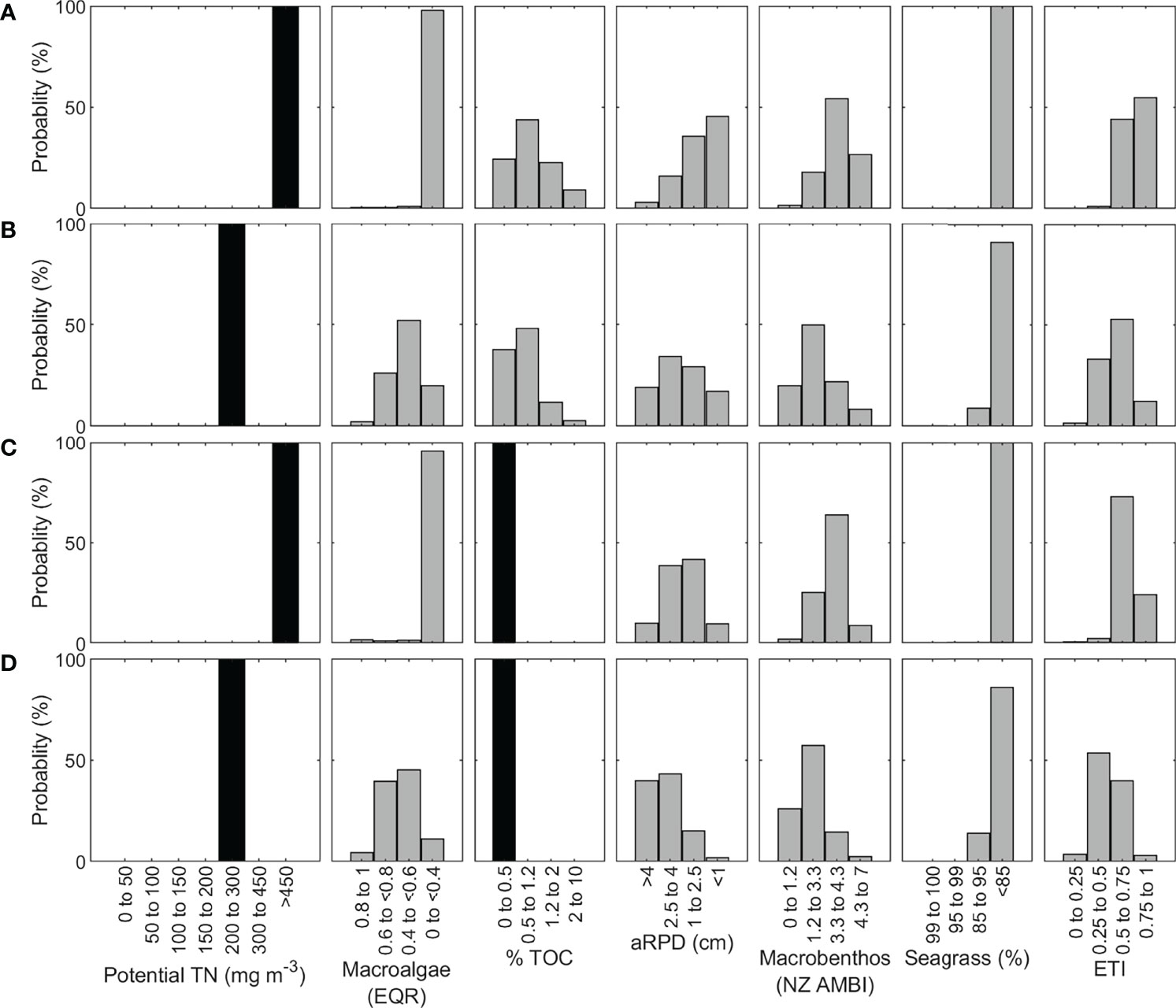
Figure 7 Avon Heathcote Estuary ETI Tool 3 BBN results for (A) pre-wastewater diversion, (B) post-wastewater diversion, (C) pre-wastewater diversion with observed % TOC, and (D) post-wastewater diversion with observed % TOC. Black bars indicate where values have been input for each scenario, and grey bars are the distributions calculated by the BBN.

To illustrate the effects of incorporating prior knowledge of indicator values, we input field-observed, low % TOC values for the AHE (Zeldis et al., 2020) to the ETI Tool 3 BBN, for pre- and post-wastewater diversion cases (Figures 7C, D). This improved indicator scores, changing pre-diversion ETI score from predominately band D to band C, and post-diversion score from predominately band C to B. Secondary indicators were also substantially improved, particularly aRPD and NZ AMBI, for both pre- and post-diversion scenarios. This showed the capacity for the BBN to describe interactions of nutrient vs sediment effects, in this case an estuary which was eutrophic (arising from TN loading effects on macroalgae) but had ‘naturally’ low sediment organic content.

In the second case study example, the ETI Tool 3 BBN was used to estimate the nutrient load reduction required to obtain a desired (lower) ETI score. Jacobs River Estuary at Riverton, South Island, is a small (6.7 km²) shallow (mean depth ~2.2 m) mesotidal tidal lagoon which currently has high potential TN concentration (666 mg m^-3) driven by heavy agricultural diffuse loading (cf. Figure 3). Its BBN-predicted ETI score was 0.84 (Figure 8A), in good agreement with its observed ETI Tool 2 score of 0.85 (Table 3). This placed the estuary in band D (Table 1) indicating highly eutrophic conditions. The BBN predicted that all the secondary indicators (% TOC, aRPD, NZ AMBI, sea grass) were likely to be in poor condition.

FIGURE 8

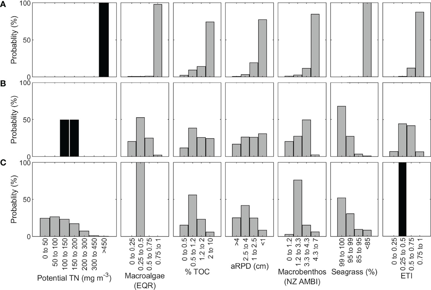
Figure 8 Jacobs River Estuary ETI Tool 3 BBN results under (A) current nutrient loading, (B) an 80% reduction in nutrient load, and (C) when setting the desired ETI score to a B band. Black bars indicate where values have been input for each scenario, and grey bars are the distributions calculated by the BBN.

The threshold to reach ETI band B is a score of ≤ 0.5. The potential TN concentration required to obtain an ETI Tool 3 BBN score of 0.5 or less can be determined in two ways: by iteratively changing the potential TN input node, or by setting the TN input node to an unspecified or unknown value and setting the ETI score to the desired value, allowing the BBN to ‘back calculate’ the required potential TN value. Figure 9A shows the response of ETI score to variation of potential TN concentration, obtained by stepping through each potential TN band in turn. The ETI score increased linearly with increasing potential TN until the highest TN band was reached (450 – 1000 mg m^-3). The non-linear response beyond 400 mg m^-3 occurred due to a combination of the ETI score having a maximum value of 1.0, and because the highest potential TN band encompasses a much wider range of potential TN concentrations than prior bands. From Figure 9A, we infer that a reduction to around 150 mg m^-3 TN (~80% reduction from current potential TN concentrations) would be required to obtain a B band. To confirm this estimate, we then set the probabilities of the potential TN bands for 100-150 and 150-200 mg m^-3 each to 50% (giving a mean potential TN concentration of 150 mg m^-3) and estimated the likely effect on the primary and secondary indicators (Figure 8B). The resulting ETI score was 0.48 ± 0.17. Compared to the present-day scenario, all secondary indicators were substantially improved.

FIGURE 9

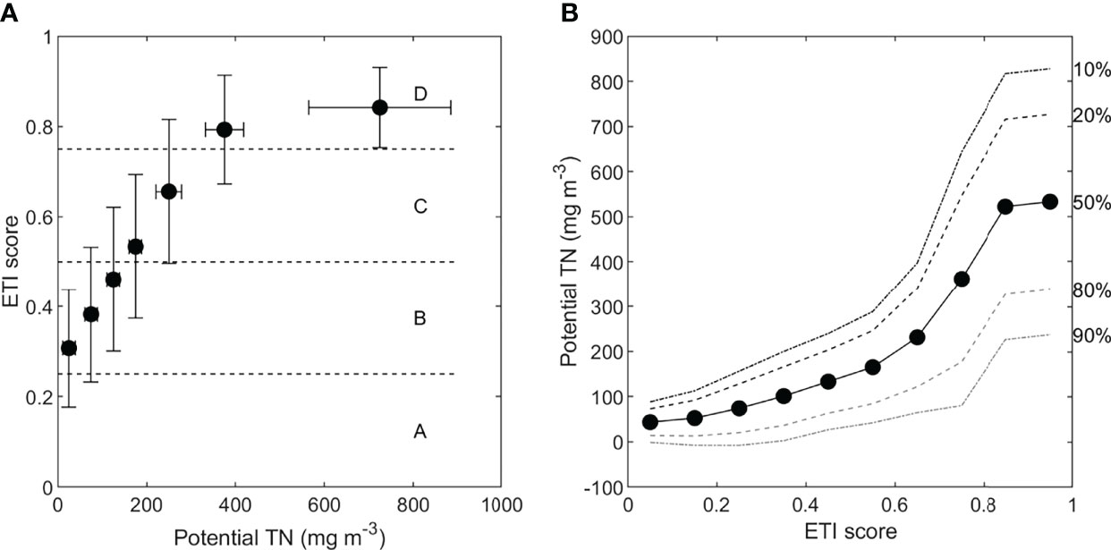
Figure 9 (A) Predicted ETI Tool 3 BBN score with increasing potential TN concentration in Jacobs River Estuary. Error bars show the standard deviation of the predicted BBN score and the potential TN concentration based on the TN band width. (B) Potential TN concentrations predicted by specifying a desired ETI score. The lines show the probability that the desired ETI score (or lower) will be obtained by a potential TN concentration, where lower ETI scores mean less eutrophication.

Figure 9B shows the potential TN concentrations predicted by the ETI Tool 3 BBN if this node is left unset, and a desired ETI score is applied for the Jacobs River case. For example, by setting the ETI score node to 0.4-0.5, the BBN predicted that a potential TN concentration of 136 mg m^-3 ( ± 83 mg m^-3) was required. It is straightforward to translate these changes in potential TN to TN load reductions, using methods of Plew et al. (2018) and as shown in Snelder et al. (2020). This load reduction was estimated to be ~85%. The probability distribution of the potential TN band can be used to infer that there is an 86% probability that the potential TN concentration will need to be reduced to below 200 mg m^-3 to obtain a B band (Figure 8C). Figure 9B also shows potential TN concentrations at which there is a 10%, 20%, 50%, 80% or 90% probability that the desired ETI score will not be exceeded for Jacobs River Estuary. For example, there is only a 10% probability of an ETI score ≤ 0.5 at a potential concentration of 264 mg m^-3.

This case study shows the use of the BBN for informing upstream limit setting for nutrients with respect to health of estuarine receiving environments. While not demonstrated here, effects of altered sediment loads may be assessed independently or in conjunction with changed nutrient loads.

4.3 International Applicability and Comparisons With Other Estuary BBNs

Eutrophication and sedimentation in estuaries are global problems (Bricker et al., 2008), with characteristic effects on estuary health. While the ETI Tool 3 BBN was developed for NZ, it has features and attributes which could enable its use elsewhere. The BBN considers a set of estuary types which are common globally, although elsewhere they may constitute differing proportions of system types than in NZ. For example, the USA southwestern coast has many lagoon-type systems, with similarities to the tidal lagoons of our study, while the USA east coast has primarily river-mouth systems in the north, with potential similarity to NZ tidal river estuaries, and lagoonal systems in the south (Bricker et al., 2008). Typologies developed for other countries (e.g., Borja et al., 2004; Bricker et al., 2008; Buddemeier et al., 2008) will be useful for understanding the applicability of this NZ estuary BBN elsewhere.

Relationships between the nodes in the ETI Tool 3 BBN were developed from studies made elsewhere, as well as in NZ, supporting its potential for application more widely. For example, the macroalgae EQR method used for evaluating macroalgal responses was based on its development within the Water Framework Directive (Borja et al., 2004; WFD-UKTAG, 2014) but, based on knowledge from California and NZ estuaries, its biomass thresholds were adjusted for the NZ context (Sutula et al., 2014; Robertson et al., 2016b; Plew et al., 2020). Phytoplankton thresholds used in the NZ context were unmodified from the Basque estuary thresholds (Revilla et al., 2010) with the exception of addition of bandings for coastal lakes. Borja et al. (2012), considering phytoplankton thresholds developed among different countries, noted that thresholds separating small from large impacts were roughly consistent. This suggested there was consistency among similar types of water bodies globally in their response to nutrient loads, as well as a global understanding of undesirable levels of phytoplankton.

There appear to be few published Bayesian models for predicting estuary health. A Bayesian approach was developed for Neuse River Estuary in eastern USA (Arhonditsis et al., 2007), targeting spatiotemporal phytoplankton dynamics in a single estuary system rather than an estuary health assessment applicable to multiple estuaries, as done here. Graham et al. (2019) applied a Bayesian modelling approach to three Queensland, Australia estuaries to predict water quality (dissolved oxygen and chl-a) and benthic biodiversity that has similarities to the ETI Tool 3 BBN, albeit developed for a small number of estuaries with a focus on predicting individual indicators rather than an overall health index. Graham et al. (2019) trained their BBN using an expectation-maximisation algorithm and case files (observations of model inputs and outputs), as they had monthly monitoring data for 5 years for each estuary. We did not have sufficient observational data spanning the range of inputs (e.g. estuary type, potential TN concentrations, flushing times), indicator values and ETI score that we employ, to use that approach. Therefore, we developed the CPTs linking the nodes using local and international studies and tested the ETI Tool 3 BBN against data available for 11 estuaries (sections 3.1 and 3.2). Bulmer et al. (2019) developed a BBN for NZ estuaries that included a wider range of indicators than the ETI Tool 3 BBN. However, relationships between nodes were based on expert opinion rather than the quantitative observational and model-based approach used here. It was not typologically resolved, included indicators not commonly or easily measured, and did not generate an overall estuary health score.

In the ETI Tool 3 BBN, we introduce capacity to provide regional or national estimates by employing geospatial tools. To apply this approach elsewhere, agencies will need to have access to these underlying resources, potentially including statistical or mechanistic catchment land-use models (Preston et al., 2011; G. Arnold et al., 2012; Elliott et al., 2016; Snelder et al., 2017). Physiographic properties of estuaries are also required, particularly estuary volume, tidal prism and intertidal area, and ideally salinity data to tune dilution models that convert the nutrient loads to potential nutrient concentrations (Plew et al., 2018). While other agencies could use our model as a starting point (https://shiny.niwa.co.nz/Estuaries-Screening-Tool-3/), other agencies should focus on ensuring that the relationships among indicators and drivers within the BBN are appropriate for their local conditions, for example relationships between potential TN and local nuisance algal species.

The ETI Tool 3 BBN is complementary to the pressure/influencing factors assessment of the ASSETS and WFD-BC approaches. Both ASSETS and WFD-BC assess the nutrient load pressure on estuaries using bandings of nutrient load modified by simple characterizations of dilution and flushing potential (Bricker et al., 1999; Garmendia et al., 2012). ASSETS was developed for large sub-tidally dominated estuaries, but over half of NZ estuaries have volumes too small to fit within the ASSETS bandings for calculating dilution potential (Plew et al., 2018). The BBN focuses on smaller estuaries, particularly tidal lagoons and tidal river estuaries. A similar issue regarding small estuary volume in the Basque region was addressed by considering a simple characterisation of mixing conditions rather than a volume-based dilution potential (Garmendia et al., 2012). The BBN uses potential nutrient concentrations (which are calculated using ETI Tool 1), which is an alternative approach of accounting for the mixing characteristics of estuaries (Plew et al., 2018).

ASSETS and WFD-BC can score an estuary’s health if observations are available. In contrast, the ETI Tool 3 BBN makes predictions of the state of individual ecological indicators as well as overall condition, from nutrient and sediment loading, without requiring observations. Observed indicator values can be added to the BBN, and we consider this most useful where only some of the indicators have been observed.

4.4 Future Development

The validation dataset we have used is small and is mainly from tidal lagoons. Future work should include more extensive surveillance of estuary health indicators, particularly for tidal rivers and coastal lakes. These data will improve parameterisations of relationships between drivers and responses to eutrophication, better accounting for estuary type, leading to more precise and accurate predictions of trophic state.

The current ETI Tool 3 BBN provides a framework to which other indicators could be added, such as metals, microphytobenthos (Berthelsen et al., 2018; Berthelsen et al., 2020; Mangan et al., 2020; Zeldis et al., 2020). The inclusion of macrophytes (in addition to seagrass) and the effects of epiphytes and phytoplankton shading (Burkholder et al., 2007) may improve the usefulness of the BBN, particularly for coastal lakes which transition from macrophyte- to phytoplankton-dominated with increasing eutrophication (Phillips et al., 2016; Schallenberg et al., 2017). The BBN considers nitrogen loading but not phosphorus because N limitation is more common in estuarine waters (NRC, 2000; Barr, 2007; Robertson and Savage, 2018) and estuarine macroalgae have high N:P requirements (Dudley et al., 2022). However, reducing phosphorus loads is commonly a successful strategy for mitigating eutrophication in freshwater lakes (Schindler et al., 2016), and including phosphorus may further improve the BBN for coastal lakes and phytoplankton dominated estuaries.

As noted (Introduction), our approach with the ETI Tool 3 BBN was to use indicators which are commonly and relatively easily measured in NZ eutrophication assessments (Robertson et al., 2016b; Robertson et al., 2017), but it could be extended to consider ecological components such as shellfish or fish (Bulmer et al., 2019; Parsons et al., 2021) or climatic effects such as marine heatwaves (Roberts et al., 2019; Straub et al., 2019; Tait et al., 2022), assuming their relationships with other BBN indicators can be adequately described. Relationships between nodes in the BBN could be further refined as data become available, either via improved empirical or mechanistic models, or by training the BBN using case learning (Graham et al., 2019).

While we describe capability to evaluate ~75% of NZ estuaries, we did not include deep bay estuaries (Introduction). Plew et al. (2020) predicted that most NZ deep bay estuaries have low or moderate susceptibility to eutrophication, particularly the large, deep systems in Fiordland (southwestern South Island) and many large coastal bays. However, some deep bays backed by catchments with higher degrees of land-use intensification require attention. This includes the Firth of Thames in northern North Island, which is susceptible to phytoplankton eutrophication and exhibits phytoplankton-driven hypoxia and pH depression (Zeldis and Swaney, 2018; Zeldis et al., 2022), arising from poor water quality of its contributing rivers. However, generating input data for deep bays, such as flushing time and potential nutrient concentration, will require more complex models than the simple dilution models in ETI Tool 1. Also, our knowledge of the interactions of phytoplankton with secondary indicators in deep bays are not presently sufficient, and would need further work.

5 Conclusion

The validations and case studies presented here demonstrate the utility of the ETI Tool 3 BBN. First, they show that multiple ecological indicators, as well as the final integrated BBN estuary health score, may be predicted solely based on the values of the drivers, which are readily available from ETI Tool 1 output. This means that estuary health status may be predicted from nutrient load data and estuary characteristics in the absence of within-estuary indicator values, should these not be available. The BBN has the feature of allowing the user to update indicator nodes, should such data be available, which may improve the accuracy of other indicator predictions and the final BBN health score. The case studies showed how scenarios may be tested, including how changed upstream nutrient loads from point or diffuse sources affect estuary health indices.

The ETI Tool 3 BBN has value for resource managers in that it allows users to evaluate trophic conditions across a great majority of NZ’s estuaries, particularly its small-to medium-size estuaries. Large, deep bay estuaries are currently not evaluated, and likely will require more complex, bespoke biophysical model developments. However, the current focus of the BBN on lagoon, riverine and coastal lake estuaries is beneficial, because of their often high sensitivity to eutrophication pressure, particularly for macroalgal-driven eutrophication (Plew et al., 2020).

The ETI Tool 3 BBN uses observation and model-derived data for commonly measured indicators, which quantify stressor-impact relationships. By its focus on providing overall estuary trophic scores, the BBN allows comparison of relative impact across systems within and between physiographic types, regionally or nationally, and has capacity to score absolute levels of trophic health. It has potential to be used across time, for both forecasting and retrospectively, as demonstrated by our case studies of Jacobs River and Avon-Heathcote estuaries. It can also be applied nationwide, to assess changes in estuary health accruing from land-use changes (e.g., Bricker et al., 2008). It could be used to inform estuarine management objectives and evaluate management actions to meet those objectives, such as is currently required under the NPSFM (New Zealand Government, 2020). The BBN may also serve as a template for other agencies internationally, who may wish to develop similar tools. This will depend on the availability of underlying resources, including geospatially - distributed land use/water quality models and databases of estuary physiographic parameters. The ETI Tool 3 BBN may therefore provide other agencies with both an incentive and a model for assembling such resources in a unified estuary and water quality management tool.

Data Availability Statement

Publicly available datasets were analyzed in this study. This data can be found here: https://shiny.niwa.co.nz/Estuaries-Screening-Tool-1/.

Author Contributions

JZ conceived the study. JZ and DP contributed equally to the analysis and writing of the manuscript. All authors contributed to the article and approved the submitted version.

Conflict of Interest

The authors declare that the research was conducted in the absence of any commercial or financial relationships that could be construed as a potential conflict of interest.

Publisher’s Note

All claims expressed in this article are solely those of the authors and do not necessarily represent those of their affiliated organizations, or those of the publisher, the editors and the reviewers. Any product that may be evaluated in this article, or claim that may be made by its manufacturer, is not guaranteed or endorsed by the publisher.

Acknowledgments

At NIWA we are grateful to Richard Storey for advice at initial stages of ETI Tool 3 BBN development, Amy Whitehead for assistance with ETI Tool 3 website development and Bruce Dudley for feedback on the manuscript. We thank Leigh Stevens (Salt Ecology Ltd.) for provision of estuary field data. Early development was funded through an ‘Envirolink Tools’ project of the New Zealand Ministry of Business, Innovation and Employment (MBIE) Contract C01X1420. Additional development was funded by MBIE Strategic Science Investment Funding to the National Institute of Water and Atmospheric Research (NIWA) Causes and Effects of Water Quality Degradation Programme (Project FWWQ2211).

Supplementary Material

The Supplementary Material for this article can be found online at: https://www.frontiersin.org/articles/10.3389/fmars.2022.898992/full#supplementary-material

References

Arhonditsis G. B., Paerl H. W., Valdes-Weaver L. M., Stow C. A., Steinberg L. J., Reckhow K. H. (2007). Application of Bayesian Structural Equation Modeling for Examining Phytoplankton Dynamics in the Neuse River Estuary (North Carolina, USA). Estuar. Coast. Shelf. Sci. 72 (1), 63–80. doi: 10.1016/j.ecss.2006.09.022

CrossRef Full Text | Google Scholar

Arnold J. G., Moriasi D. N., Gassman P. W., Abbaspour K. C., White M. J., Srinivasan R., et al. (2012). SWAT: Model Use, Calibration, and Validation. Trans. ASABE. 55 (4), 1491–1508. doi: 10.13031/2013.42256

CrossRef Full Text | Google Scholar

Atkinson M. J., Smith S. V. (1983). C:N:P Ratios of Benthic Marine Plants. Limnol. Oceano. 28 (3), 568–574. doi: 10.4319/lo.1983.28.3.0568

CrossRef Full Text | Google Scholar

Barr N. G. (2007). Aspects of Nitrogen Metabolism in the Green Alga Ulva: Developing an Indicator of Seawater Nitrogen Loading (Auckland: Auckland University).

Google Scholar

Barr N. G., Dudley B. D., Rogers K. M., Cornelisen C. D. (2013). Broad-Scale Patterns of Tissue-δ15n and Tissue-N Indices in Frondose Ulva Spp.; Developing a National Baseline Indicator of Nitrogen-Loading for Coastal New Zealand. Mar. pollut. Bull. 67 (1), 203–216. doi: 10.1016/j.marpolbul.2012.11.033

PubMed Abstract | CrossRef Full Text | Google Scholar

Barr N., Zeldis J., Scheuer K., Schiel D. (2020). Macroalgal Bioindicators of Recovery From Eutrophication in a Tidal Lagoon Following Wastewater Diversion and Earthquake Disturbance. Estuar. Coast. 43 (2), 240–255. doi: 10.1007/s12237-019-00654-7

CrossRef Full Text | Google Scholar

Berthelsen A., Atalah J., Clark D., Goodwin E., Patterson M., Sinner J. (2018). Relationships Between Biotic Indices, Multiple Stressors and Natural Variability in New Zealand Estuaries. Ecol. Indic. 85, 634–643. doi: 10.1016/j.ecolind.2017.10.060

CrossRef Full Text | Google Scholar

Berthelsen A., Atalah J., Clark D., Goodwin E., Sinner J., Patterson M. (2020). New Zealand Estuary Benthic Health Indicators Summarised Nationally and by Estuary Type. New Z. J. Mar. Freshw. Res. 54 (1), 24–44. doi: 10.1080/00288330.2019.1652658

CrossRef Full Text | Google Scholar

Bolton-Ritchie L., Main M. (2005). Nutrient water quality Avon-Heathcote Estuary/Ihutai: inputs, concentrations and potential effects. Environment Canterbury Technical Report, U05/71, Christchurch: Environment Canterbury, 84.

Google Scholar

Booker D. J., Woods R. A. (2014). Comparing and Combining Physically-Based and Empirically-Based Approaches for Estimating the Hydrology of Ungauged Catchments. J. Hydrol. 508, 227–239. doi: 10.1016/j.jhydrol.2013.11.007

CrossRef Full Text | Google Scholar

Borja A., Basset A., Bricker S., Dauvin J.-C., Elliot M., Harrison T., et al. (2012). “Classifying Ecological Quality and Integrity of Estuaries,” in Treatise on Estuarine and Coastal Science. Eds. Wolanski E., McLusky D. (Waltham, MA: Academic Press), 125–162.

Google Scholar

Borja A., Franco J., Pérez V. (2000). A Marine Biotic Index to Establish the Ecological Quality of Soft-Bottom Benthos Within European Estuarine and Coastal Environments. Mar. pollut. Bull. 40 (12), 1100–1114. doi: 10.1016/S0025-326X(00)00061-8

CrossRef Full Text | Google Scholar

Borja Á., Franco J., Valencia V., Bald J., Muxika I., Jesús Belzunce ,., et al. (2004). Implementation of the European Water Framework Directive From the Basque Country (Northern Spain): A Methodological Approach. Mar. Pollut. Bull. 48 (3), 209–218. doi: 10.1016/j.marpolbul.2003.12.001

PubMed Abstract | CrossRef Full Text | Google Scholar

Bricker S. B., Clement C. G., Pirhalla D. E., Orlando S. P., Farrow D. R. G. (1999). National Estuarine Eutrophication Assessment: Effects of Nutrient Enrichment in the Nation's Estuaries (Silver Spring, MD: NOAA, National Ocean Service, Special Projects Office, and the National Centers for Coastal Ocean Science), 71.

Google Scholar

Bricker S. B., Ferreira J. G., Simas T. (2003). An Integrated Methodology for Assessment of Estuarine Trophic Status. Ecol. Model. 169 (1), 39–60. doi: 10.1016/S0304-3800(03)00199-6

CrossRef Full Text | Google Scholar

Bricker S. B., Longstaff B., Dennison W., Jones A., Boicourt K., Wicks C., et al. (2008). Effects of Nutrient Enrichment in the Nation's Estuaries: A Decade of Change. Harm. Algae. 8 (1), 21–32. doi: 10.1016/j.hal.2008.08.028

CrossRef Full Text | Google Scholar

Buddemeier R. W., Smith S. V., Swaney D. P., Crossland C. J., Maxwell B. A. (2008). Coastal Typology: An Integrative “Neutral” Technique for Coastal Zone Characterization and Analysis. Estuar. Coast. Shelf. Sci. 77 (2), 197–205. doi: 10.1016/j.ecss.2007.09.021

CrossRef Full Text | Google Scholar

Bulmer R. H., Stephenson F., Lohrer A., Hewitt J. E. (2019). “Exploring the Impact of Multiple Stressors on Estuarine Ecosystems Using a Bayesian Network Model,” in NIWA Client Report: Prepared for Parliamentary Commissioner for the Environment (Hamilton: National Institute of Water and Atmospheric Research), 65.

Google Scholar

Burge P. I. (2007). “Sedimentation in the Avon-Heathcote Estuary/Ihutai - an Analysis of Past and Present Studies,” in Report Prepared for Environment Canterbury Regional Council and the Avon-Heathcote Estuary Ihutai Trust (Christchurch: University of Canterbury), 49.

Google Scholar

Burkholder J., Glasgow H. J., Cooke J. (1994). Comparative Effects of Water-Column Nitrate Enrichment on Eelgrass Zostera Marina, Shoalgrass Halodule Wrightii, and Widgeongrass Ruppia Maritima. Mar. Ecol. Prog. Ser. 105, 121–138. doi: 10.3354/meps105121

CrossRef Full Text | Google Scholar

Burkholder J. M., Tomasko D. A., Touchette B. W. (2007). Seagrasses and Eutrophication. J. Exp. Mar. Biol. Ecol. 350 (1), 46–72. doi: 10.1016/j.jembe.2007.06.024

CrossRef Full Text | Google Scholar

Clark D. E., Hewitt J. E., Pilditch C. A., Ellis J. I. (2019). The Development of a National Approach to Monitoring Estuarine Health Based on Multivariate Analysis. Mar. pollut. Bull. 150, 110602. doi: 10.1016/j.marpolbul.2019.110602

PubMed Abstract | CrossRef Full Text | Google Scholar

Cloern J. E. (1996). Phytoplankton Bloom Dynamics in Coastal Ecosystems: A Review With Some General Lessons From Sustained Investigation of San Francisco Bay, California. Rev. Geophys. 34 (2), 127–168. doi: 10.1029/96RG00986

CrossRef Full Text | Google Scholar

Cloern J. E. (2001). Our Evolving Conceptual Model of the Coastal Eutrophication Problem. Mar. Ecol. Prog. Ser. 210, 223–253. doi: 10.3354/meps210223

CrossRef Full Text | Google Scholar

Cloern J. E., Jassby A. D. (2008). Complex Seasonal Patterns of Primary Producers at the Land–Sea Interface. Ecol. Lett. 11 (12), 1294–1303. doi: 10.1111/j.1461-0248.2008.01244.x

PubMed Abstract | CrossRef Full Text | Google Scholar

Conley D. J., Carstensen J., Vaquer-Sunyer R., Duarte C. M. (2009). Ecosystem Thresholds With Hypoxia. Hydrobiologia 629 (1), 21–29. doi: 10.1007/s10750-009-9764-2

CrossRef Full Text | Google Scholar

Davies-Colley R., Franklin P., Wilcock B., Clearwater S., Hickey C. (2013). “National Objectives Framework - Temperature, Dissolved Oxygen & pH Proposed Thresholds for Discussion,” in NIWA Client Report, HAM2013-056, Hamilton: National Institute of Water and Atmospheric Research (Hamilton: National Institute of Water and Atmospheric Research), 83.

Google Scholar

Duarte C. M., Krause-Jensen D. (2018). Intervention Options to Accelerate Ecosystem Recovery From Coastal Eutrophication. Front. Mar. Sci. 5 (470). doi: 10.3389/fmars.2018.00470

CrossRef Full Text | Google Scholar

Dudley B. D., Barr N. G., Plew D. R., Scheuer K. (2022). Experiments to Parametrise a Growth and Nutrient Storage Model for Agarophyton Spp. Estuar. Coast. Shelf. Sci. 264, 107660. doi: 10.1016/j.ecss.2021.107660

CrossRef Full Text | Google Scholar

Dudley B. D., Zeldis J., Burge O. (2017). “New Zealand Coastal Water Quality Assessment,” in NIWA Report to Ministry for the Environment (Christchurch, New Zealand: National Institute of Water and Atmospheric Research).

Google Scholar

Elliott A. H., Semadeni-Davies A. F., Shankar U., Zeldis J. R., Wheeler D. M., Plew D. R., et al. (2016). A National-Scale GIS-Based System for Modelling Impacts of Land Use on Water Quality. Environ. Model. Soft. 86, 131–144. doi: 10.1016/j.envsoft.2016.09.011

CrossRef Full Text | Google Scholar

Engelsen A., Hulth S., Pihl L., Sundbäck K. (2008). Benthic Trophic Status and Nutrient Fluxes in Shallow-Water Sediments. Estuar. Coast. Shelf. Sci. 78 (4), 783–795. doi: 10.1016/j.ecss.2008.02.018

CrossRef Full Text | Google Scholar

Eppley R. W., Rogers J. N., McCarthy J. J. (1969). Half-Saturation Constants for Uptake of Nitrate and Ammomium by Marine Phytoplankton. Limnol. Oceano. 14 (6), 912–920. doi: 10.4319/lo.1969.14.6.0912

CrossRef Full Text | Google Scholar

Eyre B. D., Ferguson A. J. P. (2009). Denitrification Efficiency for Defining Critical Loads of Carbon in Shallow Coastal Ecosystems. Hydrobiologia 629 (1), 137–146. doi: 10.1007/s10750-009-9765-1

CrossRef Full Text | Google Scholar

Ferreira J. G., Wolff W. J., Simas T. C., Bricker S. B. (2005). Does Biodiversity of Estuarine Phytoplankton Depend on Hydrology? Ecol. Model. 187 (4), 513–523. doi: 10.1016/j.ecolmodel.2005.03.013

CrossRef Full Text | Google Scholar

Fowler D., Coyle M., Skiba U., Sutton M. A., Cape J. N., Reis S., et al. (2013). The Global Nitrogen Cycle in the Twenty-First Century. Philos. Trans. R. Soc. B. 368 (1621), 20130164. doi: 10.1098/rstb.2013.0164

CrossRef Full Text | Google Scholar

Gadd J., Dudley B., Montgomery J., Whitehead A., Measures R., Plew D. (2020). “Water Quality of Estuary of the Heathcote and Avon Rivers / Ihutai,” in NIWA Client Report: Prepared for Environment Canterbury (Auckland: National Institute of Water and Atmospheric Research), 108.

Google Scholar

Garmendia M., Bricker S., Revilla M., Borja Á., Franco J., Bald J., et al. (2012). Eutrophication Assessment in Basque Estuaries: Comparing a North American and a European Method. Estuar. Coast. 35 (4), 991–1006. doi: 10.1007/s12237-012-9489-8

CrossRef Full Text | Google Scholar

Gerwing T. G., Cox K., Gerwing A. M. A., Carr-Harris C. N., Dudas S. E., Juanes F. (2018). Depth to the Apparent Redox Potential Discontinuity (aRPD) as a Parameter of Interest in Marine Benthic Habitat Quality Models. Int. J. Sed. Res. 33 (2), 149–156. doi: 10.1016/j.ijsrc.2017.09.001

CrossRef Full Text | Google Scholar

Gibbs M. M., Vant W. N. (1997). Seasonal Changes in Factors Controlling Phytoplankton Growth in Beatrix Bay, New Zealand. New Z. J. Mar. Freshw. Res. 31 (2), 237–248. doi: 10.1080/00288330.1997.9516761

CrossRef Full Text | Google Scholar

Graham S. E., Chariton A. A., Landis W. G. (2019). Using Bayesian Networks to Predict Risk to Estuary Water Quality and Patterns of Benthic Environmental DNA in Queensland. Integ. Environ. Assess. Manage. 15 (1), 93–111. doi: 10.1002/ieam.4091

CrossRef Full Text | Google Scholar

Gray J. S., Wu R.-s., Or Y. Y. (2002). Effects of Hypoxia and Organic Enrichment on the Coastal Marine Environment. Mar. Ecol. Prog. Ser. 238, 249–279. doi: 10.3354/meps238249

CrossRef Full Text | Google Scholar

Green L., Sutula M., Fong P. (2014). How Much is Too Much? Identifying Benchmarks of Adverse Effects of Macroalgae on the Macrofauna in Intertidal Flats. Ecol. Appl. 24 (2), 300–314. doi: 10.1890/13-0524.1

PubMed Abstract | CrossRef Full Text | Google Scholar

Harding L. W., Batiuk R. A., Fisher T. R., Gallegos C. L., Malone T. C., Miller W. D., et al. (2014). Scientific Bases for Numerical Chlorophyll Criteria in Chesapeake Bay. Estuar. Coast. 37 (1), 134–148. doi: 10.1007/s12237-013-9656-6

CrossRef Full Text | Google Scholar

Hicks M., Semadeni-Davies A., Haddadchi A., Shankar U., Plew D. (2019). “Updated Sediment Load Estimator for New Zealand,” in NIWA Client Report: Prepared for Ministry for the Environment (Christchurch: National Institute of Water and Atmospheric Research), 190.

Google Scholar

Howarth R. W. (2008). Coastal Nitrogen Pollution: A Review of Sources and Trends Globally and Regionally. Harm. Algae. 8 (1), 14–20. doi: 10.1016/j.hal.2008.08.015

CrossRef Full Text | Google Scholar

Howarth R. W., Marino R. (2006). Nitrogen as the Limiting Nutrient for Eutrophication in Coastal Marine Ecosystems: Evolving Views Over Three Decades. Limnol. Oceano. 51 (1part2), 364–376. doi: 10.4319/lo.2006.51.1_part_2.0364

CrossRef Full Text | Google Scholar

Huettel M., Rusch A. (2000). Advective Particle Transport Into Permeable Sediments ­- Evidence From Experiments in an Intertidal Sandflat. Limnol. Oceano. 45 (3), 525–533. doi: 10.4319/lo.2000.45.3.0525

CrossRef Full Text | Google Scholar

Hughes B. B., Haskins J. C., Wasson K., Watson E. (2011). Identifying Factors That Influence Expression of Eutrophication in a Central California Estuary. Mar. Ecol. Prog. Ser. 439, 31–43. doi: 10.3354/meps09295

CrossRef Full Text | Google Scholar

Hume T. (2018). “Fit of the ETI Trophic State Susceptibility Typology to the NZ Coastal Hydrosystems Classification,” in NIWA Client Report (Christchurch: National Institute of Water and Atmospheric Research), 34.

Google Scholar

Hume T., Gerbeaux P., Hart D., Kettles H., Neale D. (2016). “A Classification of New Zealand's Coastal Hydrosystems,” in NIWA Client Report: Prepared for Ministry of the Environment (Hamilton: National Institute of Water and Atmospheric Research), 120.

Google Scholar

Hume T. M., Snelder T., Weatherhead M., Liefting R. (2007). A Controlling Factor Approach to Estuary Classification. Ocean. Coast. Manage. 50 (11–12), 905–929. doi: 10.1016/j.ocecoaman.2007.05.009

CrossRef Full Text | Google Scholar

Hyland J., Balthis L., Karakassis I., Magni P., Petrov A., Shine J., et al. (2005). Organic Carbon Content of Sediments as an Indicator of Stress in the Marine Benthos. Mar. Ecol. Prog. Ser. 295, 91–103. doi: 10.3354/meps295091

CrossRef Full Text | Google Scholar

Inglis G. J. (2003). “Seagrasses of New Zealand,” in World Atlas of Seagrasses. Eds. Green E. P., Short F. T. (Berkeley CA: University of California Press), 134–143.

Google Scholar

Jones H. F. E., Pilditch C. A., Bruesewitz D. A., Lohrer A. M. (2011). Sedimentary Environment Influences the Effect of an Infaunal Suspension Feeding Bivalve on Estuarine Ecosystem Function. PLoS One 6 (10), e27065. doi: 10.1371/journal.pone.0027065

PubMed Abstract | CrossRef Full Text | Google Scholar

Katwijk M., Vergeer L. H. T., Schmitz G. H. W., Roelofs J. G. M. (1997). Ammonium Toxicity in Eelgrass Zostera Marina. Mar. Ecol. Prog. Ser. 157, 159–173. doi: 10.3354/meps157159

CrossRef Full Text | Google Scholar

Lehninger A. L. (1975). Biochemistry (New York: Worth Publishers).

Google Scholar

Lohrer A. M., Hewitt J. E., Thrush S. F. (2006). Assessing Far-Field Effects of Terrigenous Sediment Loading in the Coastal Marine Environment. Mar. Ecol. Prog. Ser. 315, 13–18. doi: 10.3354/meps315013

CrossRef Full Text | Google Scholar

Lohrer A. M., Thrush S. F., Gibbs M. M. (2004). Bioturbators Enhance Ecosystem Function Through Complex Biogeochemical Interactions. Nature 431 (7012), 1092–1095. doi: 10.1038/nature03042

PubMed Abstract | CrossRef Full Text | Google Scholar

Mangan S., Bryan K. R., Thrush S. F., Gladstone-Gallagher R. V., Lohrer A. M., Pilditch C. A. (2020). Shady Business: The Darkening of Estuaries Constrains Benthic Ecosystem Function. Mar. Ecol. Prog. Ser. 647, 33–48. doi: 10.3354/meps13410

CrossRef Full Text | Google Scholar

Martins I., Oliveira J. M., Flindt M. R., Marques J. C. (1999). The Effect of Salinity on the Growth Rate of the Macroalgae Enteromorpha Intestinalis (Chlorophyta) in the Mondego Estuary (West Portugal). Acta Oecolog. 20 (4), 259–265. doi: 10.1016/S1146-609X(99)00140-X

CrossRef Full Text | Google Scholar

Monbet Y. (1992). Control of Phytoplankton Biomass in Estuaries: A Comparative Analysis of Microtidal and Macrotidal Estuaries. Estuaries 15 (4), 563–571. doi: 10.2307/1352398

CrossRef Full Text | Google Scholar

Morrison M., Lowe M., Parsons D., Usmar N., McLeod I. (2009). “A Review of Land-Based Effects on Coastal Fisheries and Supporting Biodiversity in New Zealand,” in New Zealand Aquatic Environment and Biodiversity Report 37 (Wellington: New Zealand Ministry of Fisheries), 100.

Google Scholar

Newton A. C. (2009). “"Bayesian Belief Networks in Environmental Modelling: A Review of Recent Progress,",” in Environmental Modelling Research. Eds. Findlay P. N. (Hauppauge, New York, USA: Nova Science Publishers), 13–50.

Google Scholar

New Zealand Government (2020). National Policy Statement for Freshwater Management (Wellington: Ministry for the Environment).

Google Scholar

Norsys (2005) NeticaTM Application: A Complete Software Application to Solve Problems Using Bayesian Belief Networks and Influence Diagrams. Available at: http://www.norsys.com (Accessed 2019).

Google Scholar

NRC (2000). Clean Coastal Waters Understanding and Reducing the Effects of Nutrient Pollution (Washington DC: National Academy Press).

Google Scholar

Parsons D. M., Hartill B. W., Broekhuizen N., McKenzie J. R., Stephenson F., Petersen G. L., et al. (2021). Integrating Multi-Disciplinary Data Sources Relating to Inshore Fisheries Management via a Bayesian Network. Ocean. Coast. Manage. 208, 105636. doi: 10.1016/j.ocecoaman.2021.105636

CrossRef Full Text | Google Scholar

Pelletier M. C., Campbell D. E., Ho K. T., Burgess R. M., Audette C. T., Detenbeck N. E. (2011). Can Sediment Total Organic Carbon and Grain Size be Used to Diagnose Organic Enrichment in Estuaries? Environ. Toxicol. Chem. 30 (3), 538–547. doi: 10.1002/etc.414

PubMed Abstract | CrossRef Full Text | Google Scholar

Phillips G., Willby N., Moss B. (2016). Submerged Macrophyte Decline in Shallow Lakes: What Have We Learnt in the Last Forty Years? Aquat. Bot. 135, 37–45. doi: 10.1016/j.aquabot.2016.04.004

CrossRef Full Text | Google Scholar

Plew D. R., Zeldis J. R., Dudley B. D., Whitehead A. L., Stevens L. M., Robertson B. M., et al. (2020). Assessing the Eutrophic Susceptibility of New Zealand Estuaries. Estuar. Coast. 43, 2015–2033. doi: 10.1007/s12237-020-00729-w

CrossRef Full Text | Google Scholar

Plew D. R., Zeldis J. R., Shankar U., Elliott A. H. (2018). Using Simple Dilution Models to Predict New Zealand Estuarine Water Quality. Estuar. Coast. 41 (6), 1643–1659. doi: 10.1007/s12237-018-0387-6

CrossRef Full Text | Google Scholar

Pratt D. R., Lohrer A. M., Pilditch C. A., Thrush S. F. (2014). Changes in Ecosystem Function Across Sedimentary Gradients in Estuaries. Ecosystems 17 (1), 182–194. doi: 10.1007/s10021-013-9716-6

CrossRef Full Text | Google Scholar

Preston S. D., Alexander R. B., Wolock D. M. (2011). Sparrow Modeling to Understand Water-Quality Conditions in Major Regions of the United States: A Featured Collection Introduction1. JAWRA. J. Am. Water Resour. Assoc. 47 (5), 887–890. doi: 10.1111/j.1752-1688.2011.00585.x

CrossRef Full Text | Google Scholar

Quinn J. M., Monaghan R. M., Bidwell V. J., Harris S. R. (2013). A Bayesian Belief Network Approach to Evaluating Complex Effects of Irrigation-Driven Agricultural Intensification Scenarios on Future Aquatic Environmental and Economic Values in a New Zealand Catchment. Mar. Freshw. Res. 64 (5), 460–474. doi: 10.1071/MF12141

CrossRef Full Text | Google Scholar

Revilla M., Franco J., Garmendia M., Borja Á. (2010). A New Method for Phytoplankton Quality Assessment in the Basque Estuaries (Northern Spain), Within the European Water Framework Directive. Rev. Investigación. Marina. 17 (7), 149–164.

Google Scholar

Reynolds L. K., Waycott M., McGlathery K. J., Orth R. J. (2016). Ecosystem Services Returned Through Seagrass Restoration. Restor. Ecol. 24 (5), 583–588. doi: 10.1111/rec.12360

CrossRef Full Text | Google Scholar

Robertson B. P., Gardner J. P. A., Savage C. (2015). Macrobenthic–mud Relations Strengthen the Foundation for Benthic Index Development: A Case Study From Shallow, Temperate New Zealand Estuaries. Ecol. Indic. 58, 161–174. doi: 10.1016/j.ecolind.2015.05.039

CrossRef Full Text | Google Scholar

Robertson B., Savage C. (2018). Mud-Entrained Macroalgae Utilise Porewater and Overlying Water Column Nutrients to Grow in a Eutrophic Intertidal Estuary. Biogeochemistry 139 (1), 53–68. doi: 10.1007/s10533-018-0454-x

CrossRef Full Text | Google Scholar

Robertson B. P., Savage C., Gardner J. P. A., Robertson B. M., Stevens L. M. (2016c). Optimising a Widely-Used Coastal Health Index Through Quantitative Ecological Group Classifications and Associated Thresholds. Ecol. Indic. 69, 595–605. doi: 10.1016/j.ecolind.2016.04.003

CrossRef Full Text | Google Scholar

Robertson B. M., Stevens L., Robertson B., Zeldis J., Green M., Madarasz-Smith A., et al. (2016a). NZ Estuary Trophic Index Screening Tool 1. Determining eutrophication susceptibility using physical and nutrient load data. Prepared for Environlink Tools Project: Estuarine Trophic Index, MBIE/NIWA Contract No: C01X1420, 47.

Google Scholar

Robertson B. M., Stevens L., Robertson B., Zeldis J., Green M., Madarasz-Smith A., et al. (2016b). NZ Estuary Trophic Index Screening Tool 2. Determining monitoring indicators and assessing estuary trophic state. Prepared for Environlink Tools Project: Estuarine Trophic Index, MBIE/NIWA Contract No: COX1420, 68.

Google Scholar

Robertson B. M., Stevens L. M., Ward N., Robertson ,. B. P. (2017). “Condition of Southland’s Shallow, Intertidal Dominated Estuaries in Relation to Eutrophication and Sedimentation: Output 1: Data Analysis and Technical Assessment - Habitat Mapping, Vulnerability Assessment and Monitoring Recommendations Related to Issues of Eutrophication and Sedimentation,” in Report Prepared for Environment Southland (Nelson: Wriggle Coastal Management), 172.

Google Scholar

Roberts S. D., Van Ruth P. D., Wilkinson C., Bastianello S. S., Bansemer M. S. (2019). Marine Heatwave, Harmful Algae Blooms and an Extensive Fish Kill Event During 2013 in South Australia. Front. Mar. Sci. 6 (610). doi: 10.3389/fmars.2019.00610

CrossRef Full Text | Google Scholar

Schallenberg M., Hamilton D. P., Hicks A. S., Robertson H. A., Scarsbrook M., Robertson B., et al. (2017). Multiple Lines of Evidence Determine Robust Nutrient Load Limits Required to Safeguard a Threatened Lake/Lagoon System. New Z. J. Mar. Freshw. Res. 51 (1), 78–95. doi: 10.1080/00288330.2016.1267651

CrossRef Full Text | Google Scholar

Schindler D. W., Carpenter S. R., Chapra S. C., Hecky R. E., Orihel D. M. (2016). Reducing Phosphorus to Curb Lake Eutrophication is a Success. Environ. Sci. Technol. 50 (17), 8923–8929. doi: 10.1021/acs.est.6b02204

PubMed Abstract | CrossRef Full Text | Google Scholar

Scott D., Baisden T., Preston N., Trustrum N., Davies-Colley R., Woods R., et al. (2004). “High Riverine Transport of Particulate Organic Carbon in New Zealand: Potential Significance of Soil Erosion to Carbon Accounting,” in SuperSoil 2004: 3rd Australian New Zealand Soils Conference (University of Sydney, Australia: The Regional Institute).

Google Scholar

Scully M. E. (2016). The Contribution of Physical Processes to Inter-Annual Variations of Hypoxia in Chesapeake Bay: A 30-Yr Modeling Study. Limnol. Oceano. 61 (6), 2243–2260. doi: 10.1002/lno.10372

CrossRef Full Text | Google Scholar

Semadeni-Davies A., Jones-Todd C., Srinivasan M. S., Muirhead R., Elliott A., Shankar U., et al. (2020). CLUES Model Calibration and its Implications for Estimating Contaminant Attenuation. Agric. Water Manage. 228, 105853. doi: 10.1016/j.agwat.2019.105853

CrossRef Full Text | Google Scholar

Snelder T. H., Larned S. T., McDowell R. W. (2017). Anthropogenic Increases of Catchment Nitrogen and Phosphorus Loads in New Zealand. New Z. J. Mar. Freshw. Res. 2 (3), 336–361. doi: 10.1080/00288330.2017.1393758

CrossRef Full Text | Google Scholar

Snelder T. H., Whitehead A. L., Fraser C., Larned S. T., Schallenberg M. (2020). Nitrogen Loads to New Zealand Aquatic Receiving Environments: Comparison With Regulatory Criteria. New Z. J. Mar. Freshw. Res 54 (3), 527–550. doi: 10.1080/00288330.2020.1758168

CrossRef Full Text | Google Scholar

Stevens L. M. (2018a). “Fortrose (Toetoes) Estuary 2018: Broad Scale Habitat Mapping,” in Report Prepared for Environment Southland (Nelson: Wriggle Coastal Management), 50.

Google Scholar

Stevens L. M. (2018b). “Jacobs River Estuary: Broad Scale Habitat Mapping 2018,” in Report Prepared for Environment Southland (Nelson: Wriggle Coastal Management), 53.

Google Scholar

Stevens L. M. (2018c). “New River Estuary: 2018 Macroalgal Monitoring,” in Report Prepared for Environment Southland (Nelson: Wriggle Coastal Management), 29.

Google Scholar

Stevens L. M. (2018d). “Rangitikei Estuary 2018 Broad Scale Habitat Mapping,” in Report Prepared for Horizons Regoinal Council (Nelson: Wriggle Coastal Management), 32 pp.

Google Scholar

Stevens L. M. (2018e). “Tokomairiro Estuary: Broad Scale Habitat Mapping 2018,” inReport Prepared for Otago Regional Council (Nelson: Wriggle Coastal Management), 40.

Google Scholar

Stevens L. M., Forrest B. M. (2020a). “Broad Scale Intertidal Habitat Mapping of Te Awarua-O-Porirua Harbour,” in Report Prepared for Greater Wellington Regional Council, 050 (Nelson: Salt Ecology), 46.

Google Scholar

Stevens L. M., Forrest B. M. (2020b). “Te Awarua-O-Porirua Harbour Sediment Plate Monitoring 2019/2020,” in Report Prepared for Greater Wellington Regional Council (Nelson: Salt Ecology), 20.

Google Scholar

Stevens L. M., Rayes C. (2018). “Summary of the Eutrophication Susceptibility and Trophic State of Estuaries in the Tasman Region,” in Report Prepared for Tasman District Council (Nelson: Wriggle Coastal Management), 16.

Google Scholar

Stevens L. M., Robertson B. M. (2017a). “Catlins Estuary: Broad Scale Habitat Mapping 2016/17,” in Report Prepared for Otago Regional Council (Nelson: Wriggle Coastal Management), 38.

Google Scholar

Stevens L. M., Robertson B. M. (2017b). “Shag Estuary: Broad Scale Habitat Mapping 2016/17,” in Report Prepared for Otago Regional Council (Nelson: Wriggle Coastal Management), 26.

Google Scholar

Stevens L. M., Robertson B. P. (2017c). “Fortrose (Toetoes) Estuary 2016: Broad Scale Substrate, Macroalgae and Seagrass Mapping,” in Report Prepared for Environment Southland (Nelson: Wriggle Coastal Management), 29.

Google Scholar

Straub S. C., Wernberg T., Thomsen M. S., Moore P. J., Burrows M. T., Harvey B. P., et al. (2019). Resistance, Extinction, and Everything in Between – the Diverse Responses of Seaweeds to Marine Heatwaves. Front. Mar. Sci. 6 (763). doi: 10.3389/fmars.2019.00763

CrossRef Full Text | Google Scholar

Sutula M. (2011). “Review of Indicators for Development of Nutrient Numeric Endpoints in California Estuaries,” in Southern California Coastal Water Research Project Technical Report (Costa Mesa CA: Southern California Coastal Water Research Project), 269 pp.

Google Scholar

Sutula M., Bailey H., Poucher S. (2012). “Science Supporting Dissolved Oxygen Objectives in California Estuaries,” in Southern California Coastal Water Research Project Technical Report, 684 (Costa Mesa CA: Southern California Coastal Water Research Project), 86 pp.

Google Scholar

Sutula M., Green L., Cicchetti G., Detenbeck N., Fong P. (2014). Thresholds of Adverse Effects of Macroalgal Abundance and Sediment Organic Matter on Benthic Habitat Quality in Estuarine Intertidal Flats. Estuar. Coast. 37 (6), 1532–1548. doi: 10.1007/s12237-014-9796-3

CrossRef Full Text | Google Scholar

Tait L., Zeldis J., Plew D., Dudley B., Barr N., Ren J., et al. (2022). “Investigating Drivers of Macroalgal Blooms in Ihutai (Avon-Heathcote Estuary),” in NIWA Client Report (Christchurch: Prepared for Environment Canterbury), 54.

Google Scholar

Townsend M., Lohrer D. (2015). “ANZECC Guidance for Estuary Sedimentation,” in NIWA Client Report: Prepared for Ministry for the Environment, HAM2015-096 (Hamilton: National Institute of Water and Atmospheric Research), 45.

Google Scholar

Uusitalo L. (2007). Advantages and Challenges of Bayesian Networks in Environmental Modelling. Ecol. Model. 203 (3), 312–318. doi: 10.1016/j.ecolmodel.2006.11.033

CrossRef Full Text | Google Scholar

Valiela I., McClelland J., Hauxwell J., Behr P. J., Hersh D., Foreman K. (1997). Macroalgal Blooms in Shallow Estuaries: Controls and Ecophysiological and Ecosystem Consequences. Limnol. Oceano. 42 (5), 1105–1118. doi: 10.4319/lo.1997.42.5_part_2.1105

CrossRef Full Text | Google Scholar

Vant W. N., Budd R. G. (1993). Phytoplankton Photosynthesis and Growth in Contrasting Regions of Manukau Harbour, New Zealand. New Z. J. Mar. Freshw. Res. 27 (3), 295–307. doi: 10.1080/00288330.1993.9516570

CrossRef Full Text | Google Scholar

Vaquer-Sunyer R., Duarte C. M. (2008). Thresholds of Hypoxia for Marine Biodiversity. Proc. Natl. Acad. Sci. 105 (40), 15452–15457. doi: 10.1073/pnas.0803833105

CrossRef Full Text | Google Scholar

Vitousek P. M., Aber J. D., Howarth R. W., Likens G. E., Matson P. A., Schindler D. W., et al. (1997). Human Alteration of the Global Nitrogen Cycle: Sources and Consequences. Ecol. Appl. 7 (3), 737–750. doi: 10.1890/1051-0761(1997)007[0737:HAOTGN]2.0.CO;2

CrossRef Full Text | Google Scholar

Wallace R. B., Baumann H., Grear J. S., Aller R. C., Gobler C. J. (2014). Coastal Ocean Acidification: The Other Eutrophication Problem. Estuar. Coast. Shelf. Sci. 148, 1–13. doi: 10.1016/j.ecss.2014.05.027

CrossRef Full Text | Google Scholar

WFD-UKTAG (2014). UKTAG Transitional and Coastal Water Assessment Method Macroalgae Opportunistic Macroalgal Blooming Tool. 24 Stirling, Water Framework Directive - United Kingdom Advisory Group.

Google Scholar

Whitehead A., Depree C., Quinn J. (2019). “Seasonal and Temporal Variations in Water Quality in New Zealand Rivers,” in NIWA Client Report: Prepared for Ministry for the Environment 2019024ch (Christchurch: National Institute of Water and Atmospheric Research), 79.

Google Scholar

Woodland R. J., Thomson J. R., Mac Nally R., Reich P., Evrard V., Wary F. Y., et al. (2015). Nitrogen Loads Explain Primary Productivity in Estuaries at the Ecosystem Scale. Limnol. Oceano. 60 (5), 1751–1762. doi: 10.1002/lno.10136

CrossRef Full Text | Google Scholar

Zabarte-Maeztu I., Matheson F., Hawes I., Manley-Harris M. (2019). “Sediment-Effect Thresholds for the Seagrass, Zostera Muelleri: A Case Study in Porirua Harbour, New Zealand,” in New Zealand Marine Sciences Society Conference (Dunedin: New Zealand Marine Sciences Society).

Google Scholar

Zeldis J. R., Currie K. I., Graham S. L., Gall M. P. (2022). Attributing Controlling Factors of Acidification and Hypoxia in a Deep, Nutrient-Enriched Estuarine Embayment. Front. Mar. Sci. 8. doi: 10.3389/fmars.2021.803439

PubMed Abstract | CrossRef Full Text | Google Scholar

Zeldis J. R., Depree C., Gongol C., South P. M., Marriner A., Schiel D. R. (2020). Trophic Indicators of Ecological Resilience in a Tidal Lagoon Estuary Following Wastewater Diversion and Earthquake Disturbance. Estuar. Coast. 43 (2), 223–239. doi: 10.1007/s12237-019-00637-8

CrossRef Full Text | Google Scholar

Zeldis J., Hicks M., Trustrum N., Orpin A., Nodder N., Probert K., et al. (2010). “New Zealand Continental Margin Fluxes,” in Carbon and Nutrient Fluxes in Continental Margins, 1 ed. Eds. Liu K., Atkinson L., Quiñones R., Talaue-McManus L. (Heidelberg: Springer Berlin), 273–287.

Google Scholar

Zeldis J., Measures R., Stevens L., Matheson F., Dudley B. (2019). “Remediation Options for Southland Estuaries,” in NIWA Client Report: Prepared for Environment Southland (Christchurch: National Institute of Water and Atmospheric Research), 73.

Google Scholar

Zeldis J., Plew D., Whitehead A., Madarasz-Smith A., Oliver M., Stevens L., et al. (2017a)The New Zealand Estuary Trophic Index (ETI) Tools: Tool 1 - Determining Eutrophication Susceptibility Using Physical and Nutrient Load Data. In: Ministry of Business, Innovation and Employment Envirolink Tools: C01x1420. Available at: https://shiny.niwa.co.nz/Estuaries-Screening-Tool-1/ (Accessed 16 Feb 2022).

Google Scholar

Zeldis J. R., Swaney D. P. (2018). Balance of Catchment and Offshore Nutrient Loading and Biogeochemical Response in Four New Zealand Coastal Systems: Implications for Resource Management. Estuar. Coast. 41 (8), 2240–2259. doi: 10.1007/s12237-018-0432-5

CrossRef Full Text | Google Scholar

Zeldis J., Whitehead A., Plew D., Madarasz-Smith A., Oliver M., Stevens L., et al. (2017b)The New Zealand Estuary Trophic Index (ETI) Tools: Tool 2 - Assessing Estuary Trophic State Using Measured Trophic Indicators. In: Ministry of Business, Innovation and Employment Envirolink Tools Contract: C01x1420. Available at: https://shiny.niwa.co.nz/Estuaries-Screening-Tool-2/ (Accessed 16 Feb 2022).

Google Scholar

Glossary

Bayesian Belief Network (BBN): A way of determining the probability of outcome X from decision Y, given knowledge and beliefs about the systems (in this case, estuaries). BBNs use probability distributions to connect linked parameters in systems (parent and child nodes), to predict outcomes of interest.

Conditional probability table (CPT): The probability of a state of a child node occurring when the state of a linked parent node is known. Estimated from known relationships or expert opinion.

Driver nodes: Nodes in the BBN that are set by the user, based on known physical and chemical states of an estuary and largely derived from ETI Tool 1.

Estuary type: the ETI toolset has adopted a simple typology specifically suited to the assessment of estuarine ecological health in New Zealand:

● Shallow intertidal dominated estuary (SIDE) (shortened to ‘tidal lagoon’ in this study),

● Shallow, short residence time tidal river and tidal river with adjoining lagoon estuary (SSRTRE) (shortened to ‘tidal river’ in this study),

● Deeper subtidal dominated, longer residence time estuary (DSDE) (shortened to ‘deep bay’ in this study),

● Freshwater dominated system (coastal lake) that is closed to the sea most of the time.

● Intermittently closed/open estuary (ICOE) is a subtype of tidal lagoon or tidal river which may open and close on a regular basis but is normally open. Differentiated from a coastal lake which is normally closed.

Estuary Trophic Index (ETI): A score of overall estuary health, determined using the ETI tools, ranging between 0 and 1 (low to high eutrophication).

ETI Tool 1: Enables users to assess susceptibility of estuaries to eutrophication based on their nutrient loads and their flushing/dilution characteristics.

ETI Tool 2: Provides an ETI score using values of monitored indicators derived from field surveys.

ETI Tool 3: Provides an ETI score via a BBN, using Tool 1 inputs and predicted values of ecological indicators identical to or like those of Tool 2. Enables users to determine estuary health in the absence of detailed knowledge of indicator states, and to scenario-test effects of management decisions.

Intermediate calculation nodes: Nodes which provide inputs to secondary indicator nodes, arising from driver nodes. Their values may also be set based on prior knowledge of their states.

Performance indicator nodes: Nodes which calculate outcome, or score, based on driver, primary and secondary indicator node outputs.

Primary indicator nodes: Nodes which calculate responses of potentially nuisance primary producers (macroalgae, phytoplankton) to the drivers. Their values may also be set based on prior knowledge of their states.

Secondary indicator nodes: Nodes which calculate estuary health ‘symptoms’, in response to inputs from primary producers or the drivers. Their values may also be set based on prior knowledge of their states.

Primary and secondary indicator score nodes: Nodes which calculate combined scores arising from values of primary and secondary indicators.

Standardised indicator nodes: Nodes which convert values resulting from each primary and secondary indicator node to a value between 0 and 1 using four equal-sized bands. This linearizes and normalises each indicator score prior to input to the primary and secondary score nodes.

Potential Nutrient Concentrations: Volume-averaged estuary nutrient concentrations that would occur in the absence of uptake by algae, or losses or gains due to non-conservative processes such as denitrification

Macroalgal EQR: an estuarine macroalgal index that combines biomass and spatial measures, derived using the Opportunistic Macroalgal Blooming Tool, modified for NZ, and calculated for the whole estuary. EQR is calculated from observations of % cover of available intertidal habitat, affected area with > 5% macroalgae cover, average biomass (wet weight), and % cover with algae > 3 cm deep

NZ AMBI: a marine benthic index to score macrobenthic health, incorporating responses to anthropogenic disturbance and ranging from very sensitive to very insensitive. It is based on the AZTI Marine Benthic Indicator (AMBI), locally calibrated for New Zealand.

% TOC: percentage of Total Organic Carbon, by weight, in sediments.

% mud: percentage of % sediment grain size less than 63 µm, by weight.

NPSFM: National Policy Statement for Freshwater Management that sets out the objectives and policies for freshwater management in New Zealand. It provides local authorities with direction on how they should manage freshwater.