Prediction of the Central Indian Ocean Mode in S2S Models

Prediction of precipitation during the Indian summer monsoon (ISM) is a persistent scientific challenge. The central Indian Ocean (CIO) mode was proposed as a subseasonal climate mode over the tropical Indian Ocean, and it has a close relation with monsoon intraseasonal oscillations (MISO) during the ISM both in observations and simulations. In this study, the prediction skill of the CIO mode in the subseasonal-to-seasonal (S2S) air–sea coupled models is examined. The ECMWF and UKMO models display significantly higher skills for up to about 2 and 3 weeks, respectively, which are longer than other S2S models. The decline of the CIO mode prediction skill is due to the reduced signal of subseasonal zonal winds at 850 hPa over the tropical central Indian Ocean (especially along the equator; 5°S–5°N, 70°E–85°E). Therefore, a better simulation of tropical subseasonal zonal winds is required to improve the CIO mode prediction in models, and the improvement will benefit a better MISO simulation and a higher prediction skill during the ISM.

Introduction

The Indian summer monsoon (ISM) typically lasts from June to September and is a key ingredient to agricultural planning and food production on the rim of the Indian Ocean (Wang et al., 2009; Goswami et al., 2010). The monsoonal precipitation during the ISM is dominated by monsoon intraseasonal oscillations (MISO) (Goswami, 2005; Shukla, 2014), which accounts for approximately 60% of total precipitation variance over the Bay of Bengal (BoB) (Goswami, 2005; Waliser, 2006). Although monsoonal precipitation during the ISM has been widely studied, the monsoonal precipitation prediction skill remains low (e.g., Wang et al., 2004; Annamalai et al., 2007; Sabeerali et al., 2013; Wang et al., 2015). Thus, insight into subseasonal variabilities over the Indian Ocean can help facilitate better simulations and predictions of the ISM.

Many efforts have been undertaken over the last few decades to develop and improve the prediction skill of climate models, from the atmosphere-only general circulation model to the more complex atmosphere–ocean coupled models. Despite several improvements in the atmosphere–ocean coupled models, the prediction of the ISM using climate models remains a challenging problem (Cherchi and Navarra, 2003; Gadgil et al., 2005; Li and Zhang, 2009; Wang et al., 2015). Interannual anomalies of seasonal mean ISM have some predictability (Gadgil and Sajani, 1998; Kang et al., 2002; Preethi et al., 2010; Rajeevan et al., 2012), due to the close relationship of the monsoonal precipitation with El Niño–Southern Oscillation (ENSO) (e.g., Kumar et al., 2006; Gill et al., 2015), the Indian Ocean Dipole-Zonal Mode (IODZM) (e.g., Murtugudde and Busalacchi, 1999; Murtugudde et al., 2000; Ashok et al., 2001; Kripalani and Kumar, 2004), and the Atlantic Niño (Pottapinjara et al., 2014). However, the domain of subseasonal-to-seasonal signals is still regarded as a “desert of predictability” (Waliser et al., 2003; Vitart et al., 2017). In particular, the importance of the subseasonal prediction capability in a multiscale “seamless” climate system has been widely recognized nowadays (e.g., Hurrell et al., 2009; Zhang, 2013). Recently, a new intraseasonal mode, namely, the central Indian Ocean (CIO) mode, was proposed that benefits the improvement of prediction deficiencies (Zhou et al., 2017a). The CIO mode is obtained with the first combined empirical orthogonal function (EOF) mode of subseasonal zonal winds at 850 hPa (referred to as U850 hereafter) and subseasonal SST anomalies over the Indian Ocean (40°E to 120°E, 20°N to 20°S). The positive phase of the CIO mode enhances the vertical shear of easterly winds, which benefits the northward or eastward propagation of subseasonal variabilities in the tropical Indian Ocean and ultimately leads to rainfall anomalies over the BoB during the ISM (Jiang et al., 2004; Kang et al., 2010; Zhou et al., 2017a; Li et al., 2021). The CIO mode index [defined by the principal component (PC) of the first EOF mode] has a high correlation with monsoonal precipitation over the BoB and is not relevant to ENSO or IOD indices (Zhou et al., 2017a; Li et al., 2020; Qin et al., 2020; Qin et al., 2021; Meng et al., 2021). Therefore, the CIO mode and its index can provide independent information which is useful for improving the prediction of monsoon precipitation during the ISM.

The subseasonal-to-seasonal (S2S) prediction project was launched in 2013, with a focus on the intraseasonal timescale. It provides a good database to understand the CIO mode processes and their predictions in a group of models, and it has served well in calibrating the forecast systems. Our earlier study (Qin et al., 2020) found that the CIO mode and its index can be well captured in most S2S air–sea coupled models on initial days, but it deteriorates with forecast time. Moreover, intercomparisons among the S2S models yield a robust evaluation of the CIO mode simulations and predictions in the state-of-the-art ocean–atmosphere coupled models, which always lead to better predictions of MISO and monsoon rainfall during boreal summer. Thus, understanding the prediction skill for the CIO mode assists to shed some light on the prediction theory of summer monsoon rainfall. In this study, we evaluate the CIO mode predictions in S2S air–sea coupled models and discover the possible reasons for improving the performance of the CIO mode. The remainder of this paper is organized as follows. Model configurations, data, and methods used in this study are introduced in Section 2. In Section 3, the assessments of the CIO mode simulations and predictions are investigated. Finally, Section 4 shows the conclusions and discussion.

Data and Statistical Techniques

Datasets

This study uses the real-time forecast products (available with a 3‐week delay) of the S2S database from 11 models (Vitart et al., 2017). The forecast time among models is different, but the integration length exceeds a month for all models. Since the air–sea interactions cannot be captured in an atmosphere-only model, the six atmosphere–ocean coupled models are selected. The general information of the S2S coupled models, such as model resolutions and output intervals, is listed in Table 1. Outputs from most models are available from 2015 to 2020, except for the United Kingdom Met Office (UKMO) and Météo-France/Centre National de Recherche Météorologiques (CNRM) which provide outputs from 2016 to 2020. Twice weekly or weekly outputs [e.g., the Australian Bureau of Meteorology (BoM) and European Centre for Medium-Range Weather Forecasts (ECMWF)] are interpolated to daily data (Blu et al., 2004). Before the intercomparison among different models, all variables are interpolated to a horizontal resolution of 1° latitude × 1° longitude, which has no impacts on the extraction of intraseasonal variabilities in this study. All subseasonal anomalies are obtained with a 20–100-day band-pass Butterworth filter (Selesnick and Burrus, 1998) so that all synoptic, seasonal, and longer variabilities are removed.

TABLE 1

Table 1 List of S2S models used in this study.

To assess the quality of simulations and predictions, daily SST data are obtained from the National Oceanic and Atmospheric Administration (NOAA) Optimum Interpolated SST (OISST; Reynolds et al., 2007) with a resolution of 0.25° latitude × 0.25° longitude. Daily precipitation is obtained from the Tropical Rainfall Measuring Mission (TRMM 3B42 product) rainfall data with a resolution of 0.25° latitude × 0.25° longitude (Kummerow et al., 1998). Wind velocities are from the daily US National Centers for Environmental Prediction (NCEP)-National Center for Atmospheric Research (NCAR) (Kalnay et al., 1996) with a horizontal resolution of 2.5° × 2.5°.

Statistical Techniques

The method of projection is applied to evaluate the simulated CIO mode in S2S models. The SST and U850 anomalies in S2S models are projected to the spatial structure of positive CIO mode (Figure 1A). The purpose of the projection method is to extract the signals that are linearly related to the CIO mode at a specific time in each model. Then, the simulated CIO mode indices in S2S models are obtained from the projection at different lead times. The projected CIO mode index is calculated as

$$index\left(t\right)=\sum _{i,j}X\left(i,j\right)\times Y\left(i,j,t\right)\dots \left(1\right)$$

FIGURE 1

Figure 1 (A) The central Indian Ocean (CIO) mode pattern obtained by applying combined EOF analysis to daily NCEP-NCAR reanalysis and OISST during the period of 2000–2020. Colors denote the SST mode (°C): reddish for positive and bluish for negative. Contours denote the zonal wind node (m/s): solid contours for positive (westerly winds) and dashed contours for negative (easterly winds). (B) Correlation map of subseasonal precipitation during the Indian summer monsoon (ISM) with the CIO mode index. Contours represent the standard deviation of subseasonal precipitation (mm) during boreal summer, and its spacing interval is 2 mm.

where X(i, j) represents the spatial structure of the observed CIO mode (Figure 1A); Y is the combined matrix of SST and U850 anomalies; i and j are the indices of latitude and longitude, respectively; and t represents time.

The correlations, root mean square errors (RMSEs), amplitude errors, and phase errors are used to evaluate the prediction skill of the projected CIO indices in the S2S models. The amplitude errors are calculated by $\frac{\overline{A_{model}-A_{obs}}}{A_{model}}$, where A_model and A_obs represent the amplitudes of forecast and observation, respectively. The phase errors represent the differences of phase speed between forecast and observation. The signal-to-noise ratio (SNR) [$\frac{Var\left(signal\right)+Var\left(noise\right)}{Var\left(noise\right)}$] (Trenberth, 1984; Trenberth, 1985; Goswami, 2004) is used to investigate the predictability of the atmospheric and oceanic variables related to the CIO mode. Var(signal) and Var(noise) represent the variance of subseasonal anomaly and the residual variability (containing the variability of a low-pass filter of 100 days and a high-pass filter of 20 days), respectively.

Results

The CIO Mode and Its Processes

The CIO mode is captured as the first combined EOF mode of subseasonal SST anomalies and subseasonal U850 anomalies over the tropical Indian Ocean. Previous studies proved that the spatial structure and the time series of the CIO mode using different reanalysis products are robust (Zhou et al., 2017a; Qin et al., 2020). The CIO mode obtained with OISST and NCEP-NCAR reanalyses during the period of 2000–2020 is shown in Figure 1A. For the positive CIO mode, warm SST anomalies over the tropical Indian Ocean coexist with an anticyclonic circulation in the lower troposphere. The corresponding principal component (PC) of EOF1 is defined as the CIO mode index. The CIO mode index has a high correlation with the subseasonal monsoonal rainfall during the ISM over the BoB (10°N–20°N, 85°E–100°E; Figure 1B), where the average and standard deviation (STD) of monsoonal rainfall is large.

The subseasonal precipitation is poorly simulated in S2S models. For example, the variance of subseasonal precipitation averaged over the BoB (10°N–20°N, 85°E–100°E) is 46 mm² day⁻² in observations, but it is underestimated at control forecasts in S2S models (y-axis of Figure 2). Figure 2 shows the scatter plots of the variance of the subseasonal precipitation in the northern BoB (averaged within 10°N–20°N and 85°E–95°E) with respect to the variance of the projected CIO mode index in each model. The variance of subseasonal precipitation has an obvious positive correlation with the variance of the CIO mode index in all models (higher than 0.5, all the correlation coefficients are significant at 95% confidence level). It indicates that a better reproduction of the CIO mode index is favorable for capturing the strength of monsoonal precipitation in models. Moreover, the projected CIO mode index also has a high positive correlation with the monsoon precipitation over the BoB in S2S models (not shown, similar to Figure 1B). Hence, the prediction skill of the CIO mode index is an indication to the prediction of ISM, and a comprehensive evaluation on the former can shed light on the latter.

FIGURE 2

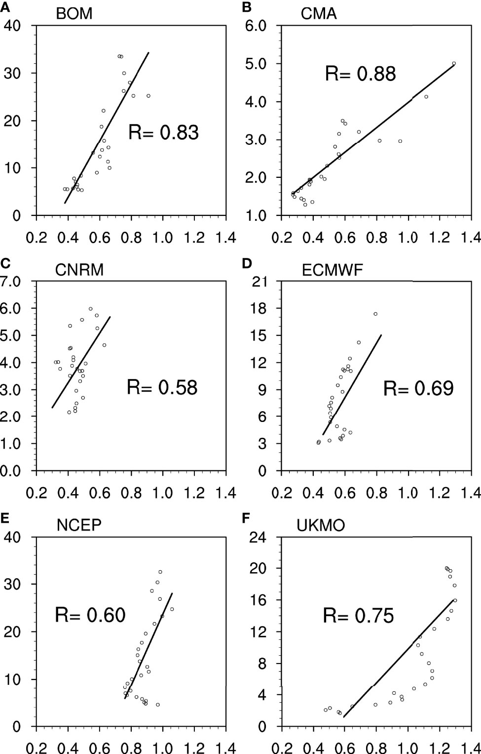
Figure 2 Scatter plots of the variance of the subseasonal precipitation in the northern BoB (averaged within 10°N–20°N and 85°E–95°E) with respect to the variance of the projected CIO mode index obtained from the (A) BoM, (B) CMA, (C) CNRM, (D) European Centre for Medium-Range Weather Forecasts (ECMWF), (E) NCEP, and (F) United Kingdom Met Office (UKMO). All results are obtained from lead time 1 to 27 days in the subseasonal-to-seasonal (S2S) models during the ISM. The black line is the linear regressions of the scatter plot.

To explore the prediction of the CIO mode index in S2S models, Figures 3A, B show the evolution of the correlation and RMSEs of the projected CIO mode indices by control forecasts for each model as a function of the lead forecast time during the ISM. The correlation is calculated with the observed CIO mode index. According to Figure 3A, the correlations can reach 0.8 on initial days in each model, but the correlation in the CNRM (yellow line) firstly shows an obvious decline after 4 days. Besides, the BoM (black line), China Meteorological Administration (CMA) (blue line), and NCEP (gray line) have similar results, which present a rapid decrease after 1 week. In contrast, the ECMWF (red line) and UKMO (green line) show higher correlations after 1 week than the other models, although their correlations are not the highest on initial days.

FIGURE 3

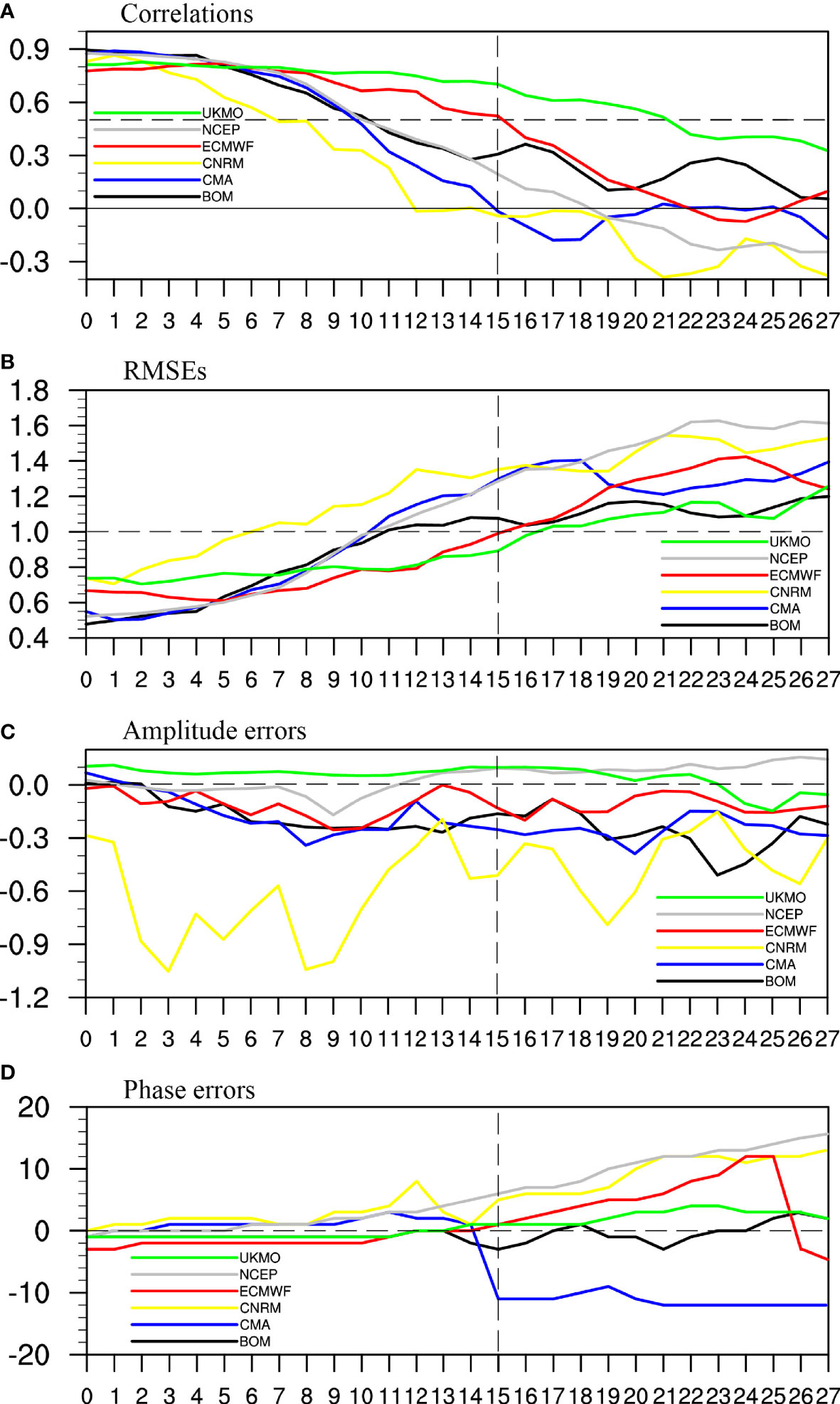
Figure 3 (A) The correlations, (B) RMSEs, (C) amplitude errors, and (D) phase errors, as a function of lead time for the projected CIO mode index from S2S models with the observed CIO mode index during the ISM for the period of 2015–2020.

The correlation coefficient of 0.5 is commonly used as the threshold for the practically useful forecast. The prediction skill score is defined as the longest lead time when the correlation drops down to 0.5. The skill scores of control forecast and ensemble means in each model are shown in Figure 4. The CIO mode skill scores from control forecast and ensemble means vary widely among models. Control forecasts (red bars) from the ECMWF and UKMO have a longer prediction up to 15 and 21 days, respectively. In comparison, the skill scores of control forecast in the BoM, CMA, and NCEP are around 10 days, while the correlation firstly becomes under 0.5 after 8 days in the CNRM (yellow line in Figure 3A). In ensemble means (gray bars in Figure 4), the CIO mode index can be predicted by the ensemble means in the ECMWF and UKMO 18 and 21 days in advance. The ensemble means skill scores show an enhancement in the BoM, ECMWF, and NCEP compared with the control forecast, whereas only slight improvements are displayed in the CNRM. In particular, both control forecast and ensemble means show that the ECMWF and UKMO models have a statistically significant lead in the CIO mode predictive skill compared with all the other S2S models. The model intercomparison based on ensemble mean may be affected by large differences in ensemble size between models (listed in Table 1). A larger ensemble size may favor a higher forecast skill. In order to get a more accurate intercomparison of the dynamical models, the control forecast (instead of ensemble mean) is used to further evaluate the performance skill of the CIO mode prediction for each model.

FIGURE 4

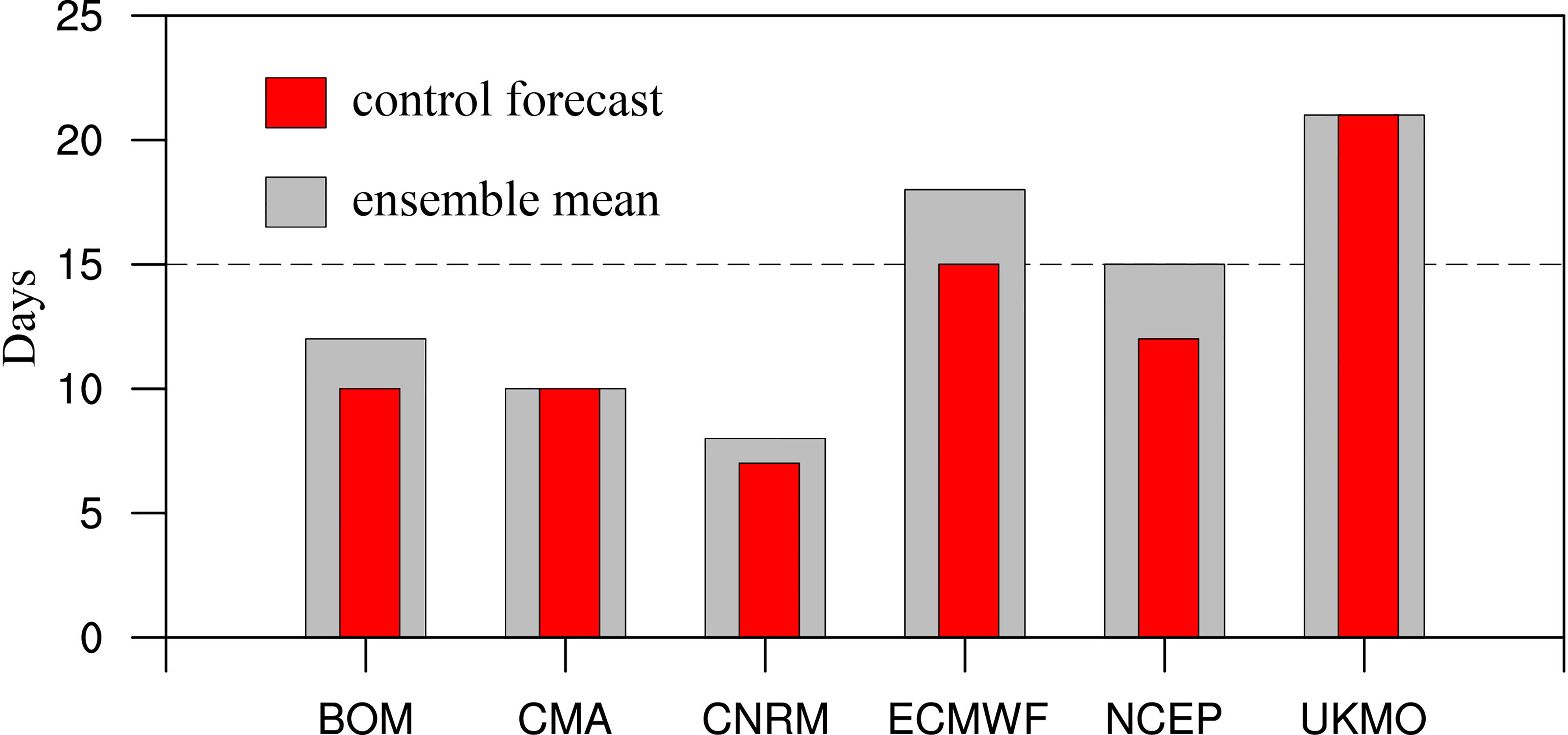
Figure 4 Forecast lead time (in days) when the CIO mode index correlation in the model ensemble means (gray bars) and control forecast (red bars) reaches 0.5.

These results are also confirmed by examining the RMSEs (Figure 3B) of the control forecast for the projected CIO mode index. The differences of RMSEs are small on initial days among S2S models (vary from 0.45 to 0.75), but the RMSE is the highest in the CNRM (yellow line) at the majority of forecast times. The ECMWF (red line) and UKMO (green line) also have relatively smaller RMSE than the other models during the forecast time of 7 to 15 days, although the RMSE is higher than the BoM (black line), CMA (blue line), and NCEP (gray line) before 1 week. The RMSE of 1.0 (black dashed horizontal lines in Figure 3B) is used as the criterion for practical useful forecast. The RMSEs for the S2S models reach 1.0 when the lead times are between 7 and 17 days. Although the RMSEs increase rapidly with the lead time, the ECMWF and UKMO also display smaller RMSEs (below 1.0 before 15 days) than the other models. Figure 3C shows the errors of the projected CIO mode index amplitude as a function of lead time during boreal summer. The majority of the S2S models produce a weaker amplitude of the CIO mode than observations, by up to about 30% of the CIO mode index amplitude in almost all models. It indicates the underestimated CIO mode events and related monsoon rainfall in S2S models. However, some models (the NCEP and UKMO) produce stronger CIO mode events at lead times than observations. Figure 3D shows the phase errors of the CIO mode index in S2S models. The positive (negative) phase errors represent the slow (fast) northward propagation of MISO and late (early) monsoon precipitation relative to observations. The phase errors are negligible before 2 weeks but clearly increase after 15 days in all models, resulting in a relatively slowly propagating MISO. The prediction of the CIO mode amplitude in NCEP is close to observations, but with increasing positive phase errors from the lead time of 10 days onwards, which leads to the rapid decline of correlations in NCEP (gray line in Figure 3A). Such phase errors are likely attributed to the influence of systematic errors in the tropical large-scale circulation and SSTs. Therefore, the above results suggest that the UKMO and ECMWF are more skillful in the prediction of the CIO mode than the other models.

Possible Reasons for Better Prediction of the CIO Mode

Because of the better performance of the ECMWF and UKMO, these two models are used to further discover the reason for the decreasing prediction skill of the CIO mode at forecast times. The prediction skill of the CIO mode has also deteriorated within 4 weeks in the ECMWF and UKMO. The first EOF mode of subseasonal SST and U850 from the control forecast is further examined. The simulated CIO mode at the lead time day 1 and day 15 is basically similar to the observations (Figure 1A), associated with warm SST anomalies over the tropical Indian Ocean and an anticyclonic circulation in the lower troposphere. Figure 5 shows the pattern differences between the observed CIO mode and simulated CIO mode (the first EOF mode of subseasonal SST and U850 in models) from the control forecasts at lead time day 1 and day 15 in the ECMWF and UKMO. One can see that the biases of the first EOF mode at lead time of day 1 are relatively small, and their patterns are similar to the biases at day 15. The SSTs are warmer in the tropical South Indian Ocean and colder in the South China Sea in the ECMWF and UKMO, which are likely attributable to initial values. The difference of U850 is negligible at lead time of day 1 (Figures 5A, C), but generally becomes greater as the forecast time increases. The positive values are located in the eastern tropical Indian and Pacific Oceans and the Arabian Sea, while the negative values are located over the BoB and the tropical South Indian Ocean (Figures 5C, D). This suggests that the main biases of winds may originate from the model dynamical or physical processes with forecast times, rather than the model initial value biases.

FIGURE 5

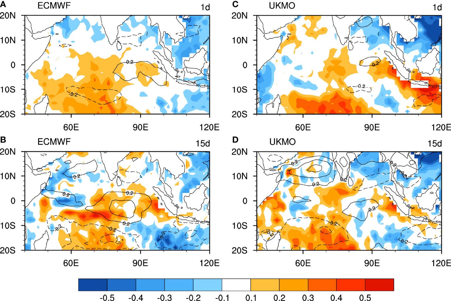
Figure 5 (A) Difference maps between the CIO mode of observation and the ECMWF forecast at a day 1 lead time. Colors denote the SST node (°C), and contours denote the zonal wind node (m/s). (B) The same as (A), but for the day 15 lead time. (C, D) The same as (A) and (B), but for the UKMO.

The downdraft associated with the deep convection over the western Pacific warm pool is the trigger for positive SST anomalies in the central Indian Ocean during the positive CIO mode (Zhou et al., 2017a). To compare the importance of atmospheric and oceanic variables, SST and U850 in the ECMWF and UKMO are replaced with observation and reanalysis for projection, respectively. Figure 6 shows the correlations in the ECMWF (red lines) and UKMO (green lines) during the ISM for the period of 2015–2020. The projected CIO mode index obtained by the model SST and U850 from NCEP-NCAR shows a higher performance skill in the prediction of the CIO mode (dashed lines, over 0.8 for forecast times). In contrast, the projected CIO mode index obtained by OISST and U850 in models has no obvious difference with Figure 3A (solid lines). Therefore, it is speculated that the increasing bias of U850 is the main reason for the decreasing prediction skill of the CIO mode in models.

FIGURE 6

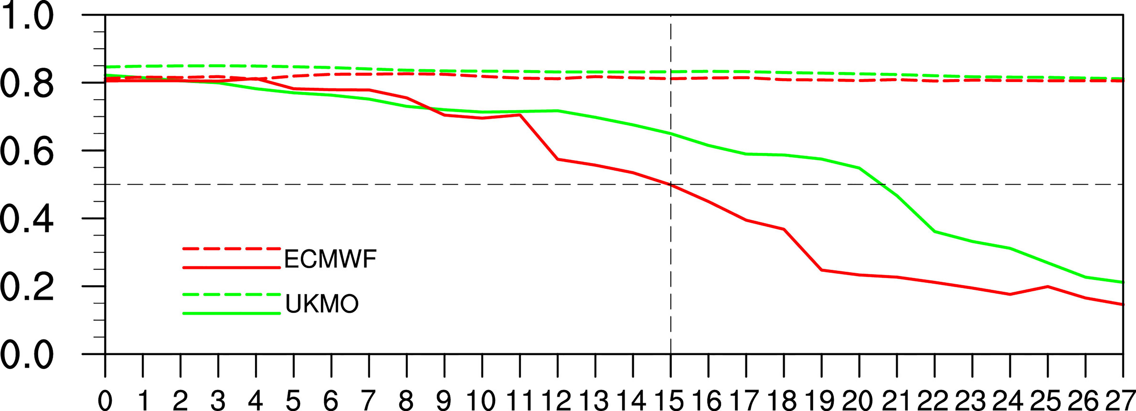
Figure 6 The correlations in the ECMWF (red lines) and UKMO (green lines) during the ISM for the period of 2015–2020. The dashed lines are calculated with the SST from the S2S model data and U850 from NCEP-NCAR. The solid lines are calculated with the U850 from the S2S model data and OISST.

To further explore the bias of U850, Figure 7A shows the SNR as a function of lead time obtained with the ECMWF and UKMO. The SNR method has been widely used to investigate atmospheric predictability (Trenberth, 1984; Trenberth, 1985; Goswami, 2004; Li et al., 2019). The SNR of U850 is calculated averaged in the tropical Indian Ocean (20°S–20°N, 40°E–120°E), which is the area for the production of the CIO mode. Such SNR value represents the strength of zonal winds on subseasonal timescale. It can be seen that the subseasonal variance and SNRs of U850 in the UKMO (solid lines) are slightly higher than those in the ECMWF (dashed lines). Consistent with the subseasonal variance (red lines), the SNRs (black lines) of U850 show decreased trends at forecast times both in the ECMWF and UKMO and are smaller than that in reanalysis (1.33) after 1 week, indicating the gradual reduction of predictability in the tropical Indian Ocean. It is reasonably deduced that the U850 will eventually lose predictability when lead time is long enough.

FIGURE 7

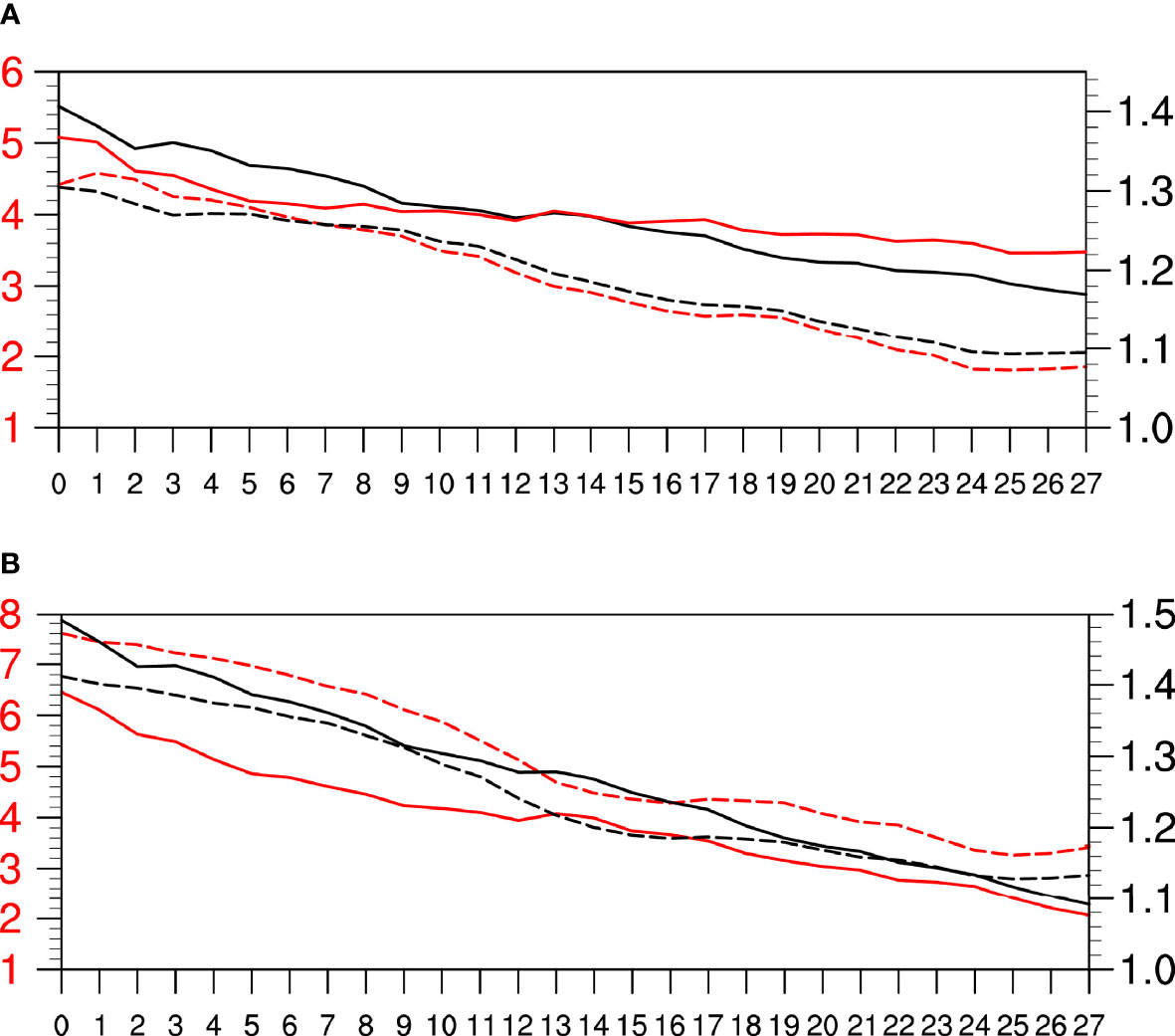
Figure 7 The variance (red lines; m² s⁻²) and SNR (black lines) of subseasonal (A) U850 and (B) U200 in the ECMWF (dashed lines) and UKMO (solid lines) over the tropical Indian Ocean (20°S–20°N, 40°E–120°E) during boreal summer for the period of 2015–2020.

To further discover the spatial pattern of decreased subseasonal zonal winds, Figure 8 shows the trends of SNRs of U850 from initial days to the lead time of 30 days over the tropical Indian Ocean in the ECMWF and UKMO. Consistent with Figure 7A, the SNR of U850 trends to negative values over almost all tropical Indian Ocean. It is also evident that the SNR becomes lower as lead time gets longer, basically due to the weakening of the signal. Particularly, the trend of SNR shows a center over 5°S–5°N, 70°E–85°E, where the easterly wind shear related to the CIO mode is important for the shift of the propagation of subseasonal variabilities (Zhou et al., 2017b). It indicates that the equatorial U850 is of the lowest predictability and is the key factor for the decreased prediction skill of the CIO mode in models. The U850 gradually becomes weaker with time over the equatorial central Indian Ocean and eventually is not strong enough for the growth of the CIO mode after 2 weeks. As a result, the inactive subseasonal zonal winds reduce the easterly wind shear along the equator and the northward propagation of MISO at forecast times, which ultimately cuts down the monsoonal precipitation in models.

FIGURE 8

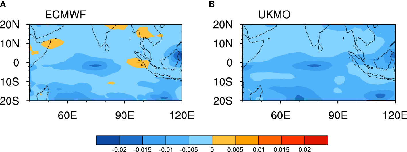
Figure 8 The trends of SNR of U850 from initial days to the lead time of 30 days over the tropical Indian Ocean in the (A) ECMWF and (B) UKMO.

Conclusions and Discussion

The CIO mode was proposed as a subseasonal mode over the Indian Ocean with a close relation to MISO and the monsoonal precipitation during the ISM. The S2S database provides a unique way to evaluate the CIO mode simulation and prediction in multiple models. Models produce weaker monsoon precipitation over the BoB than that in nature and also tend to simulate MISO propagating northward too slowly in the extended range, which are attributable to a poor rendition of the CIO mode. The intercomparison in S2S air–sea coupled models shows that the CIO mode skill scores vary widely between models. The UKMO model displays significantly higher skill scores (up to about 3 weeks) with lower RMSEs, amplitude, and phase errors in the S2S models. The ECMWF and NCEP show skill to predict the CIO mode evolution around 2 weeks, but the phase error grows rapidly in NCEP. It is revealed that the bias of subseasonal U850 plays a more important role in the decreased performance skill of the CIO mode prediction than oceanic variability in models. The strength of subseasonal U850 is reduced over the tropical central Indian Ocean (especially over 5°S–5°N, 70°E–85°E), leading to the inactive CIO mode at forecast time in the ECMWF and UKMO models.

Furthermore, the simulated signal of the subseasonal zonal wind fields at 200 hPa (U200) is examined using the SNR method (Figure 7B). Such result is similar to the U850, that is, the SNR of U200 decreases with time in models. As suggested by Jiang et al. (2004), the northward or eastward propagation of intraseasonal oscillation in the tropical Indian Ocean is closely dependent on the vertical shear of easterly winds. Thus, it is reasonable to assume that the phase errors may result from the improperly simulated easterlies in the upper troposphere.

Both observations and model simulations show that the CIO mode and the associated processes have a close relation with heavy precipitation during the ISM. For model simulations, current results indicate that a better representation of the CIO mode in S2S air–sea coupled models can be expected to improve both thermodynamic processes and dynamic circulation, which will in turn contribute to improving the MISO and ISM simulations. Actually, the predictability limit of the CIO mode can reach 38 days, which is close to the upper predictability limit of monsoonal precipitation (Qin et al., 2022). There still remains a lot of room for improvement in climate models. The relation between the CIO mode and MISO requires further explorations, which can shed more light on the role that the CIO mode plays during the ISM, both in nature and model simulations. Numerical experiments may provide us with a better chance to understand the CIO mode and the importance of barotropic instability and subseasonal zonal winds over the tropical Indian Ocean for the CIO mode generation.

Data Availability Statement

The original contributions presented in the study are included in the article/supplementary material. Further inquiries can be directed to the corresponding author.

Author Contributions

JQ, LZ, BL, and ZM contributed to the conception and design of the study. All authors contributed to the article and approved the submitted version.

Funding

This work was supported by grants from the National Natural Science Foundation of China (42106003, 42076001, 42125601), the Fundamental Research Funds for the Central Universities (B210202142), Innovation Group Project of Southern Marine Science and Engineering Guangdong Laboratory (Zhuhai) (No. 311020004), and the Oceanic Interdisciplinary Program of Shanghai Jiao Tong University (SL2020PT205). The S2S data are available from the ECMWF at https://apps.ecmwf.int/datasets/data/s2s/ and CMA at http://s2s.cma.cn/. All reanalysis products and observation data for this paper are properly cited and referred to in the reference list. NCEP-NCAR reanalysis is available at https://www.esrl.noaa.gov/psd/data/gridded/data.ncep.reanalysis.html. OISST reanalysis is available at https://www.ncdc.noaa.gov/oisst. TRMM 3B42 product observation data are available at https://gpm.nasa.gov/data-access/downloads/trmm.

Conflict of Interest

The authors declare that the research was conducted in the absence of any commercial or financial relationships that could be construed as a potential conflict of interest.

Publisher’s Note

All claims expressed in this article are solely those of the authors and do not necessarily represent those of their affiliated organizations, or those of the publisher, the editors and the reviewers. Any product that may be evaluated in this article, or claim that may be made by its manufacturer, is not guaranteed or endorsed by the publisher.

References

Annamalai H., Hamilton K., Sperber K. R. (2007). The South Asian Summer Monsoon and its Relationship With ENSO in the IPCC AR4 Simulations. J. Climate 20 (6), 1071–1092. doi: 10.1175/JCLI4035.1

CrossRef Full Text | Google Scholar

Ashok K., Guan Z., Yamagata T. (2001). Impact of the Indian Ocean Dipole on the Relationship Between the Indian Monsoon Rainfall and ENSO. Geophys. Res. Lett. 28 (23), 4499–4502. doi: 10.1029/2001GL013294

CrossRef Full Text | Google Scholar

Blu T., Thévenaz P., Unser M. (2004). Linear Interpolation Revitalized. IEEE Trans. Imag. Process. 13 (5), 710–719. doi: 10.1109/TIP.2004.826093

CrossRef Full Text | Google Scholar

Cherchi A., Navarra A. (2003). Reproducibility and Predictability of the Asian Summer Monsoon in the ECHAM4-GCM. Climate Dynam. 20 (4), 365–379. doi: 10.1007/s00382-002-0280-6

CrossRef Full Text | Google Scholar

Gadgil S., Rajeevan M., Nanjundiah R. (2005). Monsoon Prediction–Why Yet Another Failure? Curr. Sci. 88 (9), 1389–1400.

Google Scholar

Gadgil S., Sajani S. (1998). Monsoon Precipitation in the AMIP Runs. Climate Dynam. 14 (9), 659–689. doi: 10.1007/s003820050248.pdf

CrossRef Full Text | Google Scholar

Gill E. C., Rajagopalan B., Molnar P. (2015). Subseasonal Variations in Spatial Signatures of ENSO on the Indian Summer Monsoon From 1901 to 2009. J. Geophys. Res.: Atmosph. 120 (16), 8165–8185. doi: 10.1002/2015JD023184

CrossRef Full Text | Google Scholar

Goswami B. N. (2004). Interdecadal Change in Potential Predictability of the Indian Summer Monsoon. Geophys. Res. Lett. 31 (16). doi: 10.1029/2004GL020337

CrossRef Full Text | Google Scholar

Goswami B. N. (2005). “South Asian Monsoon,” in Intraseasonal Variability in the Atmosphere-Ocean Climate System (Berlin, Heidelberg: Springer), 19–61. doi: 10.1007/3-540-27250-X_2

CrossRef Full Text | Google Scholar

Goswami B. N., Kulkarni J. R., Mujumdar V. R., Chattopadhyay R. (2010). On Factors Responsible for Recent Secular Trend in the Onset Phase of Monsoon Intraseasonal Oscillations. Int. J. Climatol. 30 (14), 2240–2246. doi: 10.1002/joc.2041

CrossRef Full Text | Google Scholar

Hurrell J., Meehl G. A., Bader D., Delworth T. L., Kirtman B., Wielicki B. (2009). A Unified Modeling Approach to Climate System Prediction. Bull. Am. Meteorol. Soc. 90 (12), 1819–1832. doi: 10.1175/2009BAMS2752.1

CrossRef Full Text | Google Scholar

Jiang X., Li T., Wang B. (2004). Structures and Mechanisms of the Northward Propagating Boreal Summer Intraseasonal Oscillation. J. Climate 17 (5), 1022–1039. doi: 10.1175/1520-0442(2004)017<1022:SAMOTN>2.0.CO;2

CrossRef Full Text | Google Scholar

Kalnay E., Kanamitsu M., Kistler R., Collins W., Deaven D., Gandin L., et al. (1996). The NCEP/NCAR 40-Year Reanalysis Project. Bull. Am. Meteorol. Soc. 77 (3), 437–472. doi: 10.1175/1520-0477(1996)077<0437:TNYRP>2.0.CO;2

CrossRef Full Text | Google Scholar

Kang I.-S., Kim D., Kug J.-S. (2010): Mechanism for Northward Propagation of Boreal Summer Intraseasonal Oscillation:Convective Momentum Transport. Geophys. Res. Lett. 37, L24804, doi: 10.1029/2010GL045072

CrossRef Full Text | Google Scholar

Kang I. S., Jin K., Wang B., Lau K. M., Shukla J., Krishnamurthy V., et al. (2002). Intercomparison of the Climatological Variations of Asian Summer Monsoon Precipitation Simulated by 10 GCMs. Climate Dynam. 19 (5), 383–395. doi: 10.1007/s00382-002-0245-9

CrossRef Full Text | Google Scholar

Kripalani R. H., Kumar P. (2004). Northeast Monsoon Rainfall Variability Over South Peninsular India Vis-À-Vis the Indian Ocean Dipole Mode. Int. J. Climatol. 24, 1267–1282. doi: 10.1002/joc.1071

CrossRef Full Text | Google Scholar

Kumar K.K, Rajagopalan B., Hoerling M., Bates G., Cane M. (2006). Unraveling the Mystery of Indian Monsoon Failure During El Niño. Science 314 (5796), 115–119. doi: 10.1126/science.1131152

PubMed Abstract | CrossRef Full Text | Google Scholar

Kummerow C., Barnes W., Kozu T., Shiue J., Simpson J. (1998). The Tropical Rainfall Measuring Mission (TRMM) Sensor Package. J. Atmosph. Ocean. Technol. 15 (3), 809–817. doi: 10.1175/1520-0426(1998)015<0809:TTRMMT>2.0.CO;2

CrossRef Full Text | Google Scholar

Li B., Ding R., Qin J., Zhou L., Hu S., Li J. (2019). Interdecadal Changes in Potential Predictability of the Summer Monsoon in East Asia and South Asia. Atmosph. Sci. Lett. 20 (4), e890. doi: 10.1002/asl.890

CrossRef Full Text | Google Scholar

Li J., Zhang L. (2009). Wind Onset and Withdrawal of Asian Summer Monsoon and Their Simulated Performance in AMIP Models. Climate Dynam. 32 (7), 935–968. doi: 10.1007/s00382-008-0465-8

CrossRef Full Text | Google Scholar

Li B., Zhou L., Qin J., Murtugudde R. (2021). The Role of Vorticity Tilting in Northward-Propagating Monsoon Intraseasonal Oscillation. Geophys. Res. Lett. 48 (13), e2021GL093304. doi: 10.1029/2021GL093304

CrossRef Full Text | Google Scholar

Li B., Zhou L., Wang C., Gao C., Qin J., Meng Z. (2020). Modulation of Tropical Cyclone Genesis in the Bay of Bengal by the Central Indian Ocean Mode. J. Geophys. Res.: Atmosph. 125 (12), e2020JD032641. doi: 10.1029/2020JD032641

CrossRef Full Text | Google Scholar

Meng Z, Zhou L, Murtugudde R, Yang Q, Pujiana K, Xi J (2021). Tropical Oceanic Intraseasonal Variabilities Associated With Central Indian Ocean Mode. Clim Dy. doi: 10.1007/s00382-021-05951-1

CrossRef Full Text | Google Scholar

Murtugudde R., Busalacchi A. J. (1999). Interannual Variability of the Dynamics and Thermodynamics of the Tropical Indian Ocean. J. Climate 12, 2300–2326. doi: 10.1175/1520-0442(1999)012<2300:IVOTDA>2.0.CO;2

CrossRef Full Text | Google Scholar

Murtugudde R., McCreary J. P. Jr, Busalacchi A. J. (2000). Oceanic Processes Associated With Anomalous Events in the Indian Ocean With Relevance to 1997–1998. J. Geophys. Res.: Ocean. 105 (C2), 3295–3306. doi: 10.1029/1999JC900294

CrossRef Full Text | Google Scholar

Pottapinjara V., Girishkumar M. S., Ravichandran M., Murtugudde R. (2014). Influence of the Atlantic Zonal Mode on Monsoon depressions in the Bay of Bengal During Boreal Summer. J. of Geophys. Res.: Atmosph. 119, 6456–6469. doi: 10.1002/2014JD021494

CrossRef Full Text | Google Scholar

Preethi B., Kripalani R. H., Kumar K. K. (2010). Indian Summer Monsoon Rainfall Variability in Global Coupled Ocean-Atmospheric Models. Climate Dynam. 35 (7), 1521–1539. doi: 10.1007/s00382-009-0657-x

CrossRef Full Text | Google Scholar

Qin J., Zhou L., Ding R., Li B. (2022). Predictability Limit of Monsoon Intraseasonal Precipitation: An Implication of Central Indian Ocean Mode. Front. Mar. Sci. 8. doi: 10.3389/fmars.2021.809798

PubMed Abstract | CrossRef Full Text | Google Scholar

Qin J., Zhou L., Li B., Murtugudde R. (2020). Simulation of Central Indian Ocean Mode in S2S Models. J. Geophys. Res.: Atmosph. 125 (21), e2020JD033550. doi: 10.1029/2020JD033550

CrossRef Full Text | Google Scholar

Qin J., Zhou L., Meng Z., Li B., Lian T., Murtugudde R. (2021). Barotropic Energy Conversion During Indian Summer Monsoon: Implication of Central Indian Ocean Mode Simulation in CMIP6. Climate Dynam. doi: 10.1007/s00382-021-06087-y

CrossRef Full Text | Google Scholar

Rajeevan M., Unnikrishnan C. K., Preethi B. (2012). Evaluation of the ENSEMBLES Multi-Model Seasonal Forecasts of Indian Summer Monsoon Variability. Climate Dynam. 38, 2257–2274. doi: 10.1007/s00382-011-1061-x

CrossRef Full Text | Google Scholar

Reynolds R. W., Smith T. M., Liu C., Chelton D. B., Casey K. S., Schlax M. G. (2007). Daily High-Resolution-Blended Analyses for Sea Surface Temperature. J. Climate 20 (22), 5473–5496. doi: 10.1175/2007JCLI1824.1

CrossRef Full Text | Google Scholar

Sabeerali C. T., Ramu Dandi A., Dhakate A., Salunke K., Mahapatra S., Rao S. A. (2013). Simulation of Boreal Summer Intraseasonal Oscillations in the Latest CMIP5 Coupled GCMs. J. Geophys. Res.: Atmosph. 118 (10), 4401–4420. doi: 10.1002/jgrd.50403

CrossRef Full Text | Google Scholar

Selesnick I. W., Burrus C. S. (1998). Generalized Digital Butterworth Filter Design. IEEE Trans. Signal Process. 46 (6), 1688–1694. doi: 10.1109/78.678493

CrossRef Full Text | Google Scholar

Shukla R. P. (2014). The Dominant Intraseasonal Mode of Intraseasonal South Asian Summer Monsoon. J. Geophys. Res.: Atmosph. 119 (2), 635–651. doi: 10.1002/2013JD020335

CrossRef Full Text | Google Scholar

Trenberth K. E. (1984). Signal Versus Noise in the Southern Oscillation. Month. Weather. Rev. 112 (2), 326–332. doi: 10.1175/1520-0493(1984)112<0326:SVNITS>2.0.CO;2

CrossRef Full Text | Google Scholar

Trenberth K. E. (1985). Potential Predictability of Geopotential Heights Over the Southern Hemisphere. Month. Weather. Rev. 113 (1), 54–64. doi: 10.1175/1520-0493(1985)113<0054:PPOGHO>2.0.CO;2

CrossRef Full Text | Google Scholar

Vitart F., Ardilouze C., Bonet A., Brookshaw A., Chen M., Codorean C., et al. (2017). The Subseasonal to Seasonal (S2S) Prediction Project Database. Bull. Am. Meteorol. Soc. 98 (1), 163–173. doi: 10.1175/BAMS-D-16-0017.1

CrossRef Full Text | Google Scholar

Waliser D. E. (2006). “Intraseasonal Variability,” in The Asian Monsoon (Berlin, Heidelberg: Springer), 203–257. doi: 10.1007/3-540-37722-0_5

CrossRef Full Text | Google Scholar

Waliser D. E., Jin K., Kang I. S., Stern W. F., Schubert S. D., Wu M. L. C., et al. (2003). AGCM Simulations of Intraseasonal Variability Associated With the Asian Summer Monsoon. Climate Dynam. 21 (5), 423–446. doi: 10.1007/s00382-003-0337-1

CrossRef Full Text | Google Scholar

Wang B., Kang I. S., Lee J. Y. (2004). Ensemble Simulations of Asian–Australian Monsoon Variability by 11 AGCMs. J. Climate 17 (4), 803–818. doi: 10.1175/1520-0442(2004)017<0803:ESOAMV>2.0.CO;2

CrossRef Full Text | Google Scholar

Wang B., Lee J. Y., Kang I. S., Shukla J., Park C. K., Kumar A., et al. (2009). Advance and Prospectus of Seasonal Prediction: Assessment of the APCC/CliPAS 14-Model Ensemble Retrospective Seasonal Prediction, (1980–2004). Climate Dynam. 33 (1), 93–117. doi: 10.1007/s00382-008-0460-0

CrossRef Full Text | Google Scholar

Wang B., Xiang B., Li J., Webster P. J., Rajeevan M. N., Liu J., et al. (2015). Rethinking Indian Monsoon Rainfall Prediction in the Context of Recent Global Warming. Nat. Commun. 6 (1), 1–9. doi: 10.1038/ncomms8154

CrossRef Full Text | Google Scholar

Zhang C. (2013). Madden–Julian Oscillation: Bridging Weather and Climate. Bull. Am. Meteorol. Soc. 94 (12), 1849–1870. doi: 10.1175/BAMS-D-12-00026.1

CrossRef Full Text | Google Scholar

Zhou L., Murtugudde R., Chen D., Tang Y. (2017a). A Central Indian Ocean Mode and Heavy Precipitation During the Indian Summer Monsoon. J. Climate 30 (6), 2055–2067. doi: 10.1175/JCLI-D-16-0347.1

CrossRef Full Text | Google Scholar

Zhou L., Murtugudde R., Chen D., Tang Y. (2017b). Seasonal and Interannual Variabilities of the Central Indian Ocean Mode. J. Climate 30 (16), 6505–6520. doi: 10.1175/JCLI-D-16-0616.1

CrossRef Full Text | Google Scholar