 Yongdong Zhou
 Zekai Ni1
 Philip Adam Vetter
 Hongzhou Xu
 Bo Hong
 Hui Wang
 Wenshan Li
95% of researchers rate our articles as excellent or good
Learn more about the work of our research integrity team to safeguard the quality of each article we publish.
Find out more
ORIGINAL RESEARCH article
Front. Mar. Sci. , 21 June 2022
Sec. Coastal Ocean Processes
Volume 9 - 2022 | https://doi.org/10.3389/fmars.2022.878301
This article is part of the Research Topic Adapting and Building Local Resilience to Sea Level Rise Impacts on Coastlines View all 9 articles
Because of global warming, the sea level is expected to continue to rise, possibly having a significant impact on the intensities and spatial distribution characteristics of coastal storm surges. In this study, we took super typhoon Rammasun (2014) as a case study and applied the SCHISM (Semi-implicit Cross-scale Hydroscience Integrated System Model) to simulate storm surge in the northwestern South China Sea under future sea level rise (SLR) scenarios. To improve the accuracy of storm surge hindcast, we used reconstructed wind field to drive the model in which ERA5 reanalysis data were superposed on the wind field calculated from the Holland parametric cyclone model. The results show that the storm surge hindcast was significantly improved by using this reconstructed wind forcing. 2-D and 3-D model hindcast capabilities were compared; the 3-D model reproduced the storm surge better. The regional sea level projections in 2050, 2100, 2200, and 2300 for RCP 4.5 scenarios (provided by the IPCC AR6 dataset) were superposed on the original water depth as the predicted sea levels, then those depths were used in models of storm surge in the study area under a typhoon identical to Rammasun. Model results demonstrate that storm surge peaks in most sea areas decrease nearly linearly with SLR, especially in regions of high surges.
In the shallow water of a gradually sloping continental shelf, sea level is easily affected by tropical cyclones (TCs) that generate storm surge events at the seaboard and cause destructive flooding. Severe coastal storm surges can result in billions of dollars of economic damages and enormous loss of life in coastal zones. The South China Sea (SCS) is a large semienclosed marginal ocean basin with wide continental shelves in the western North Pacific, commonly crossed by TCs formed in the western North Pacific. In general, these TCs move westward to make landfall in southern China and wreak havoc along the way. Coastal areas of the SCS face multiple natural hazards that are related to TCs, including floods, storm surges, and erosion. In particular, coastal districts and counties in Hainan province and Guangdong province, which are densely populated and economically developed areas in China, experience the highest risk (Gao et al., 2014). Thus, it is vital to carry out relevant research and provide scientific support for marine disaster prevention and mitigation.
TCs have both low atmospheric pressures and strong winds. The low pressures raise sea level and the strong winds accumulate sea water along the coastline northwards of TC’s trajectory, and they together cause severe coastal storm surges. For storm surge prediction, high-resolution numerical models simulate storm-related hydrodynamic process and have proven to be successful (Shchepetkin and McWilliams, 2005). However, the accuracy of models depends on accurately high-resolution atmospheric forcing input, which is frequently simplified for efficiency (Dietrich et al., 2018). For example, Holland (1980) simulated surface pressure and wind fields with a simple parametric vortex model, which is empirically estimated from hurricane observations. This simulated method creates some deviations that limit the accuracy of surge inundation prediction. Furthermore, some parameterizations in storm surge models, such as bottom roughness, also cause some inaccuracies. This study focuses on numerical hindcast instead of predicting storm surge in real time. Setting aside concern for timeliness, herein we consider a modified method combining the parametric vortex model and the reanalysis data for higher accuracy. The simulated result of this study is valuable for long-term planning such as design of coastal engineering and harbor infrastructures (Halpin, 2006), and evaluation of economic losses after disasters.
Emphasis is placed on timeliness in numerical forecasting; thus, international major forecast systems use two-dimensional (2-D) models generally. Numerical hindcast does not require timeliness and permits the luxury of more accurate 3-D models. Previous research demonstrated that storm surge heights simulated by the 3-D model were generally higher than the 2-D simulation because 3-D modeled near-bottom velocity was lower than 2-D modeled depth-averaged velocity; this difference was attributed to bottom stress (Weisberg and Zheng, 2008). A completely fair comparison between the 2-D and 3-D models is difficult to obtain. Ideally, the simulated condition should be kept as similar as possible for the comparison of both models, but this is not strictly possible, as the 2-D models are more dependent on parameterizations than the 3-D models (Zheng et al., 2013). Based on different parameterization methods, the present study will explore the capability of the 2-D and 3-D models to predict the spatial distribution of storm surges in the northwestern SCS.
TC’s translation velocity is an important factor for storm surge height and affects the spatial distribution of storm surges. Peng et al. (2004) found that the hurricane with lower translation velocity produces higher storm surge. On the other hand, Rego and Li (2009) concluded that peak surge increased as the forward motion speed of the hurricane increased. According to the linear theory, the responses of ocean to atmospheric traveling disturbance are proportional to (1-U2/gh)-1. Thus, when the velocity of the traveling disturbance (U) approaches the propagation velocity of a long wave, storm surge becomes very large due to resonance (Proudman, 1954). Jelesnianski (1972) conducted numerical experiments with a standard hurricane over representative shelves, indicating that there is a ‘‘critical speed’’ that is greater than 30 mph (13.4 m/s). For the continental shelf of the northwestern SCS, it is valuable to evaluate the effects of varying translation velocity on coastal storm surge during a super typhoon.
The global mean sea level will continue to rise during the 21st century (IPCC, 2014). The peak surge will change with sea level rise (SLR) in different regions because of nonlinear interaction between them (Liu et al., 2018; Zhang et al., 2013). To evaluate the impact of SLR on storm surge, an accurate prediction of future SLR is necessary. However, global sea level prediction is complicated on account of many uncertainties brought by ice sheets, glaciers, thermal expansion, and land water storage. In addition, the responses of peak surge to SLR are local and always based on relative sea level at a particular location. From the perspective of estimating regional SLR, some local and regional signals also increase the complexity of the sea level estimation, including subsidence, ocean dynamics, climate variability, geodynamics, and other local factors (Oppenheimer et al., 2019). The SLR in the northwestern SCS has obvious localized characteristics (Xu et al., 2016). The local sea level in the SCS was projected for the 21st century using 24 CMIP5 models and could reach about 40.9 cm for the RCP2.6 scenario, 48.6 cm for the RCP4.5 scenario, and 64.1 cm for the RCP8.5 scenario by the end of the 21st century (Huang and Qiao, 2015). However, significant divergences between different climate system models cause great uncertainties in the evaluation of local sea levels. A linear extrapolation method of the sea level data observed by satellite altimeters was used in the Yellow Sea and combined with the ICE-6G/VM5a model to include the impact of ongoing glacial isostatic adjustment but ignored the local subsidence (Yang et al., 2021). The sixth Assessment Report (AR6) of IPCC was released on August 9, 2021 and provides consensual projections on future sea levels across the globe under a range of possible future scenarios, integrating multiple causes of SLR and providing a basis for predicting the change of peak surges in future. In this study, we consider the impact of SLR that combines all sea level change causes on peak surges in the northwestern SCS.
The structure of this paper is as follows: Section 2 describes the SCHISM model and the creation of the super typhoon Rammasun wind and pressure field. Section 3 introduces the methods to generate external forcing for the model. Sections 4 and 5 compare the performance of the 2-D and 3-D models on storm surge simulations and evaluate influence of TC’s translation velocity and SLR on peak surge simulation. The paper is concluded in Section 6.
Super typhoon Rammasun was the strongest recorded typhoon to land in China since 1949. It was generated in the western Pacific Ocean on July 7, 2014, rapidly moved westward through the Philippines into the SCS, gradually intensified to super typhoon status, and successively struck three provinces of southern China (Figure 1). The typhoon track data were downloaded from the Chinese Meteorological Administration (CMA) in the Typhoon track real-time release system of the Zhejiang Water Conservancy Department (http://typhoon.zjwater.gov.cn). These track data showed that Rammasun moved at a velocity of 20 km/h to the northeast coast of Hainan Island with wind speeds exceeding 60 m/s and a central pressure of 910 hPa at 15:00 on July 18. Then, it continued to move westward and passed over the Leizhou Peninsula of Guangdong Province and landed in Guangxi Province. Finally, it rapidly weakened to a severe tropical storm and faded away in mainland China. The track of typhoon Rammasun represents one of the most frequent TC tracks in the coastal areas of SCS. It was estimated that Rammasun caused 7.2 billion dollars of property damages and resulted in the death of 88 people (Yang et al., 2019). Thus, typhoon Rammasun was selected as an example of severe TCs. In this study, because of the hourly time resolution of typhoon track data starting on the 16th at 14:00, the model is run from 16th at 14:00 to 20th at 02:00, spanning a total of 84 h (3.5 days), covering almost the entire passage of the typhoon in the SCS.
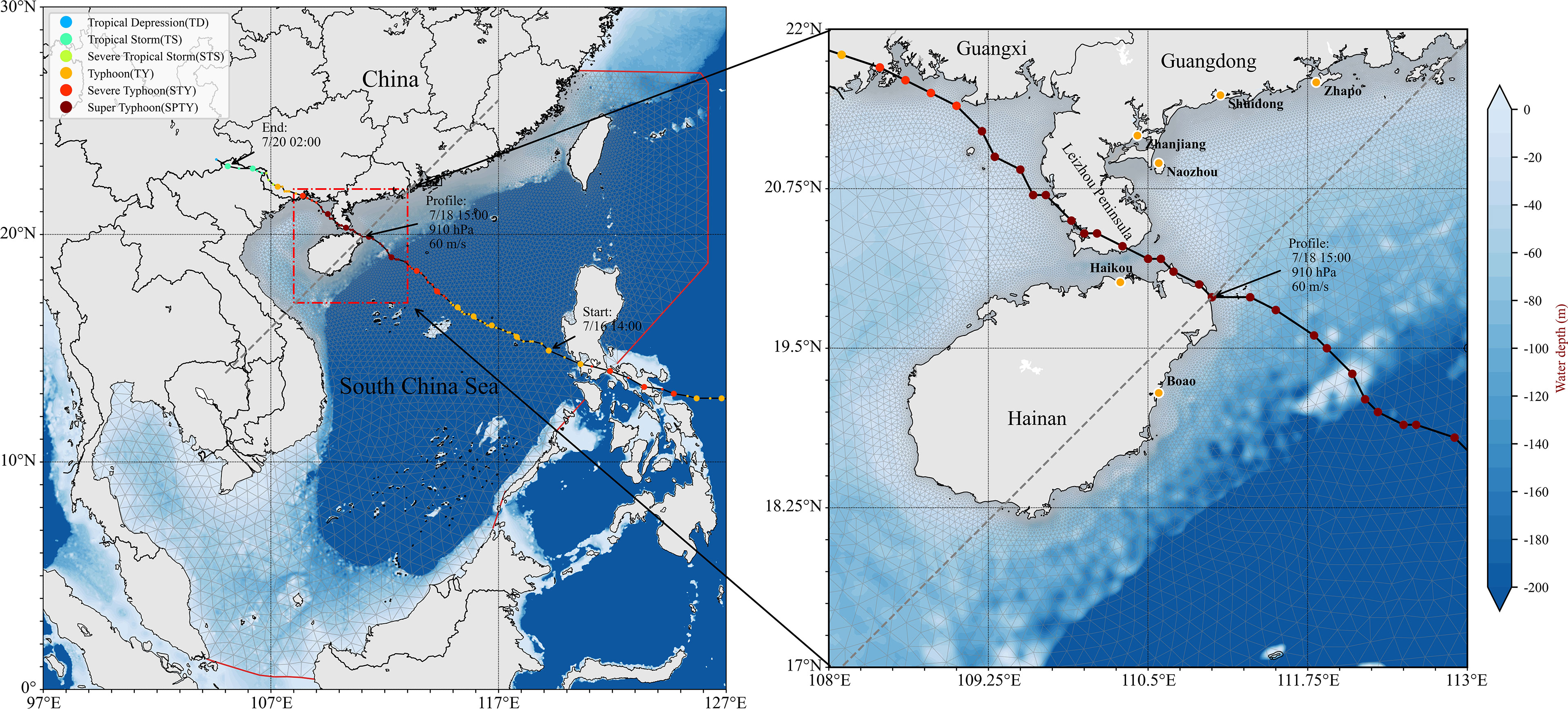
Figure 1 Bathymetry of the South China Sea and model grid (left). Black line with colored dots represents track and intensity of Typhoon Rammasun (2014). Enlarged view of the vicinity of Hainan province (Right). Yellow dots show location of six tide gauge stations (Zhapo, Shuidong, Zhanjiang, Naozhou, Haikou, and Boao stations).
Storm surge simulations were validated against observations from six tide gauges (Figure 1). The South China Sea Forecast Center, State Oceanic Administration granted hourly storm surge data recorded from 00:00 local standard time on the 17th to 10:00 local standard time on the 19th, July 2014, the 59 h from storm surge emergence to end. The entire observation period was covered in the model runtime. The capability of each model was evaluated only using those times when observations were available.
To simulate the storm surge forerunner caused by the remote wind effect at the open ocean, a large domain model grid was created as shown in Figure 1. This model domain encompasses the entire SCS and a portion of the western Pacific Ocean. Resolutions of the model grid were set to range from 200 m near the shore to 20 km at oceanic open boundaries with 212,063 nonoverlapping triangular cells and 121,113 triangular nodes to enable superior flexibility in representing the bathymetry. For the 3-D model simulations, we employed 11 uniform terrain-following S-coordinates to properly represent the bottom boundary layer in the vertical. The nearshore bathymetry data were obtained from unpublished sea charts provided by the State Oceanic Administration of China in this study. For the open sea, the water depth data of the model grid were obtained from the ETOPO1 global relief dataset with a resolution of 1 min (1.5–2 km) from NOAA (http://www.ngdc.noaa.gov/mgg/global/global.html). These datasets were interpolated into model grid nodes. The model datum was referenced to mean sea level. Open boundaries of the model run without tidal and wave forcings in this study.
The study area (17°N–22°N, 108°E–113°E) is in the northwestern region of the SCS, including Hainan Island, and a part of the coast of Guangdong and Guangxi Provinces where storm surges frequently occur. There are six tide gauge stations located along the coastline. Haikou and Boao stations are located in Hainan Island on the left side of typhoon Rammasun track and the rest of the stations are on the western coast of Guangdong Province (Figure 1).
The SLR data used in simulations is derived from the regional and local projections data provided by the IPCC 6th Assessment Report (AR6), which updates and expands the related assessments from previous reports, and provides improved projections and uncertainty estimates of future change (Fox-Kemper et al., 2021). In addition, the projections incorporate all potential processes that would affect sea level change with medium and low confidences. For the low confidence condition, the time series of the projection are up to the year 2300. The regional projections on a regular global grid are available from the NASA Sea Level Projection Tool (https://sealevel.nasa.gov/data_tools/17). In this study, we focus on four cases of future SLR by years 2050, 2100, 2200, and 2300 for the RCP 4.5 scenario (Figure 2), which relates to medium greenhouse gas emissions. To reduce the uncertainties caused by multiple contributing factors of SLR, total integrated values of all components of SLR will be selected, which contain the assessed medium-confidence and low-confidence processes (total_ssp245_low_confidence_values). Furthermore, we used the 50% quantile (median) in the range of projections from the dataset in this study. The values of regional SLR are relative to the 1995–2014 baseline, close to the occurrence time of super typhoon Rammasun (2014). The values are suitable to be directly applied to the study without further modification.
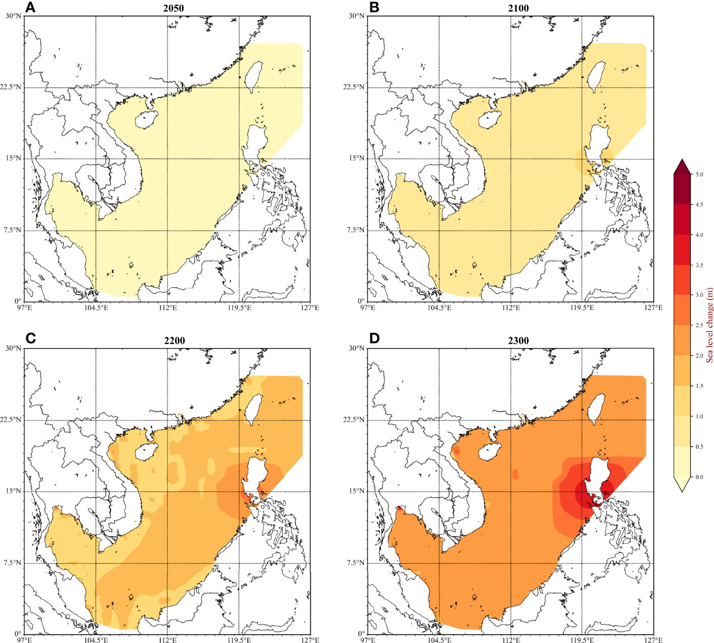
Figure 2 Predicted sea level rise in years (A) 2050, (B) 2100, (C) 2200, and (D) 2300 in the South China Sea (RCP4.5; low confidence; median).
The SCHISM model solves the standard Navier–Stokes equations with hydrostatic and Boussinesq approximations, and uses semi-implicit, finite-volume, and Eulerian–Lagrangian algorithms (Zhang et al., 2016). We executed the simulation by using the 2-D and 3-D barotropic modes of SCHISM. In 3-D mode, full 3-D cells were utilized in the entire domain with 11 vertical layers. The governing equations of the SCHISM model are composed of continuity equation and momentum equation. Continuity equation in 3-D (Eq. (1)) and 2-D depth-integrated forms (Eq. (2)) (note that bold texts in all equations represent vectors):
Momentum equation:
where vectors are expressed by using boldface type, is the horizontal gradient operator, u (x,y,z,t) is the horizontal velocity vector with Cartesian components (u,v),w is the vertical velocity, z is the vertical coordinate, n(x,y,t) is the free-surface elevation and represents storm surge height, h(x,y) is bathymetric depth, u is the depth-averaged velocity in the 2-D model, D/Dt is the material derivative, mz is the vertical eddy viscosity term, and g is the acceleration of gravity. F represents the additional forcing terms, including horizontal viscosity, Coriolis, and atmospheric pressure. The baroclinic gradient, earth tidal potential, and radiation stress are neglected in this study. The vertical eddy viscosity term mz denotes different forms in 3-D and 2-D as:
where ι is the vertical eddy viscosity and τw is the surface wind shear stress calculated based on the wind velocity vector U10 on the 10-m height above the sea surface. τb is the bottom frictional stress. ρ is the water density and Pa is the air density. H=h+n is the total water depth. As boundary conditions, τw and τb are essential for the 2-D model and the 3-D model. At the sea surface, the internal Reynolds stress is balanced by the surface wind shear stress:
Cw is the drag coefficient, which is derived from the following formula (Pond and Pickard, 2013):
At the bottom boundary layer, the internal Reynolds stress is balanced by the bottom frictional stress:
The bottom stress is also computed by a similar quadratic drag law expressed as:
The ub is the near-bottom velocity vector for the 3-D model. In this study, we calculated velocities by the 3-D model at 11 layers from the bottom of the water column to the surface, and the velocity at the first layer above the bottom represents the near-bottom velocity. However, the ub of the 2-D model is different from the 3-D model and is the depth-averaged velocity vector. In the 3-D model, the Cd is generally the bottom drag coefficient computed according to the thickness of the logarithmic bottom boundary layer:
where K is the von Karman constant (κ = 0.4) and z0 is the bottom roughness parameter, which we set to 0.02, the typical value obtained at the oceanic boundary layer (Lueck and Lu, 1997). δb is the thickness of the bottom boundary layer that is closest to the bottom. In the 2-D model, Cd may be calculated by using a function of a Manning coefficient:
where n is Manning’s friction coefficient, which could be constant or variable in 2-D flow. The 2-D model is highly dependent on the Manning coefficient, and the previous studies concluded that the temporally and spatially varying Manning coefficient may significantly improve the accuracy of the 2-D model but could cause the storm surge model to be much more cumbersome and less robust (Lapetina and Sheng, 2015). Thus, the Manning coefficient is generally set as a constant of 0.02 in the 2-D model (Xu et al., 2010; Garzon and Ferreira, 2016). In this study, we used typical values for n and z0 to compute the bottom drag coefficient under 2-D and 3-D formulations. There are significant differences of bottom drag coefficient between both formulations that may lead to different bottom stresses and have an impact on storm surge heights.
For assessment of model skill, accurately catching the peak values of storm surge is considered the criterion. Here, we calculated percentage errors (PE) of peak surge between model results and observations at six tide gauge stations to evaluate the capabilities of different wind forcings in hindcasting coastal storm surge. The formula was as follows:
where nmod and nobs are the modeled and observed peak surges, respectively. The mean absolute percentage error (MAPE) is commonly used as a measurement of simulation accuracy in model evaluation due to its very intuitive interpretation in terms of relative error. It is usually expressed as a ratio defined by the formula:
where n is the number of tide gauge stations (n = 6).
To compare time series of storm surges, model performance can be quantified with various skill metrics (Guillou, 2014; Akbar et al., 2017; Drost et al., 2017; Ding et al., 2020). The statistical errors of water surface elevations such as root-mean-square error (RMSE) and bias were frequently calculated for assessment of model capability. In this study, the metrics RMSE and bias were used to assess the absolute error between the modeled and observed values, with an ideal value of zero. In addition, Willmott skill (WS), which represented the degree of agreement, was also used for the quantitative evaluation of model performance (Willmott, 1984). A WS of 1 represents the best possible agreement between model simulation and observations, and complete disagreement was a value of 0. These metrics are calculated as follows:
where Xmod and Xobs are the modeled and observed values, respectively, and N is the number of observed samples. and are the average values. These skill metrics are adopted to test the performance of the storm surge model.
In this study, we employed a parametric vortex model to generate sea surface pressure fields and wind velocity components. The real-time track data provide the hourly location of the TC center, the central pressure, and maximum wind speed at the height of 10 m. The wind velocity used in the model is composed of rotational and translational velocities. The rotational velocity is calculated from an analytical model of the radial profiles of sea surface pressures and winds, which is proposed by Holland (1980). Holland’s model function expression is as follows:
where r is the distance from the TC center,p is the local pressure at the location of r, Pc is the central pressure, Pn is the ambient pressure (1,010 hPa), Rm is the radius of maximum wind velocity, V(r) is the gradient wind velocity at r,Pa is the air density (1.15 kg/m3), e is Euler’s number, f is the Coriolis parameter (f=2ΩsinΦ), Ω is the angular frequency of the Earth rotation, Φ is the latitude of the TC center, and B is pressure profile parameter. B can be calculated from Eq. (18) by neglecting the Coriolis parameter and setting r=Rm as follows:
where Vm is the maximum gradient of wind velocity. This method was extensively used because the required maximum wind velocity and radial pressure gradient can be easily obtained from meteorological agencies (Hu et al., 2012). However, Rm is not provided with real-time track data. To supplement this, we used the best track data that were provided by the Joint Typhoon Warning Center (JTWC) (https://www.metoc.navy.mil/jtwc/jtwc.html). In their data, the radius of maximum wind speed had a 6-h temporal resolution, which was interpolated linearly to hourly resolution in this study. The direction of wind velocity components was adjusted by the inflow angle (αF), which is about 25° outside and decreases to 0 at the TC center (Mattocks and Forbes, 2008):
To remove the impact of the TC motion, a translational velocity vector (Vmov) caused by the movement of the TC was added to the rotational velocity vector (V) for the stationary symmetric TC to create an asymmetric wind velocity vector (Ueno, 1981), and the translational velocity vector is calculated by the exponential function form:
in which Vmc is the moving velocity vector of the typhoon center. The wind field is calculated by the following formula:
where i and j are the unit vectors in the x and y directions, respectively; Vinital is the wind vector obtained from Holland’s parametric vortex model [Eq.(18)], and C1, C2 were, respectively, 1.0 and 0.8 in the parametric vortex model, which was confirmed by multiple comparative calculations (Yang and Yan, 2021).
According to previous research, the magnitude of wind simulated by the parametric vortex model decreased much faster away from the radius of maximum wind than the observed one and thus may underestimate the actual background wind (Lin and Chavas, 2012). In contrast, the reanalysis datasets are better at reconstructing the wind field in the areas farther away from the TC center but worse near the TC center (Pan et al., 2016). To improve the accuracy of the wind field, we used a combination of Holland’s parametric vortex model and the reanalysis data in this study. The method is considered to be an optimized combination of the two wind fields. We compared the combined data with single data to verify the conjecture that the combined data generally perform well.
The global ERA5 reanalysis dataset provided hourly data with a spatial resolution of 0.25°(latitude) × 0.25°(longitude) on single levels by the European Centre for Medium-Range Weather Forecasts (ECMWF) (https://cds.climate.copernicus.eu/cdsapp#!/dataset/reanalysis-era5-single-levels). A smooth transition is very important between the wind field of the parametric vortex model and the wind field obtained from the ERA5 reanalysis data (hereinafter abbreviated to ERA5 data). To avoid discontinuity between the two wind fields, we used a weighted average formula to smooth the transition between the two wind fields:
where Vc is the combined wind vector, Vb is the background wind vector from the ERA5 dataset, C is an intermediate variable, α is the weight coefficient, and n=4 (Li et al., 2020).
Figure 3 presents the horizontal wind speed profiles and spatial distributions of typhoon Rammasun when it landed on Hainan Island. The main differences between the parametric wind profile and the ERA5 wind profile were reflected in the differences in the peak wind. The Holland parametric TC model can reproduce the maximum wind speed (Vm) with >50 m/s, which was close to the observed value. However, wind speeds of ERA5 data are lower than 30 m/s and the radius of maximum wind is much larger than the radius provided by the JTWC track data. Thus, this reconstruction method was used to improve the simulated results by combining the better part of the two wind profiles.
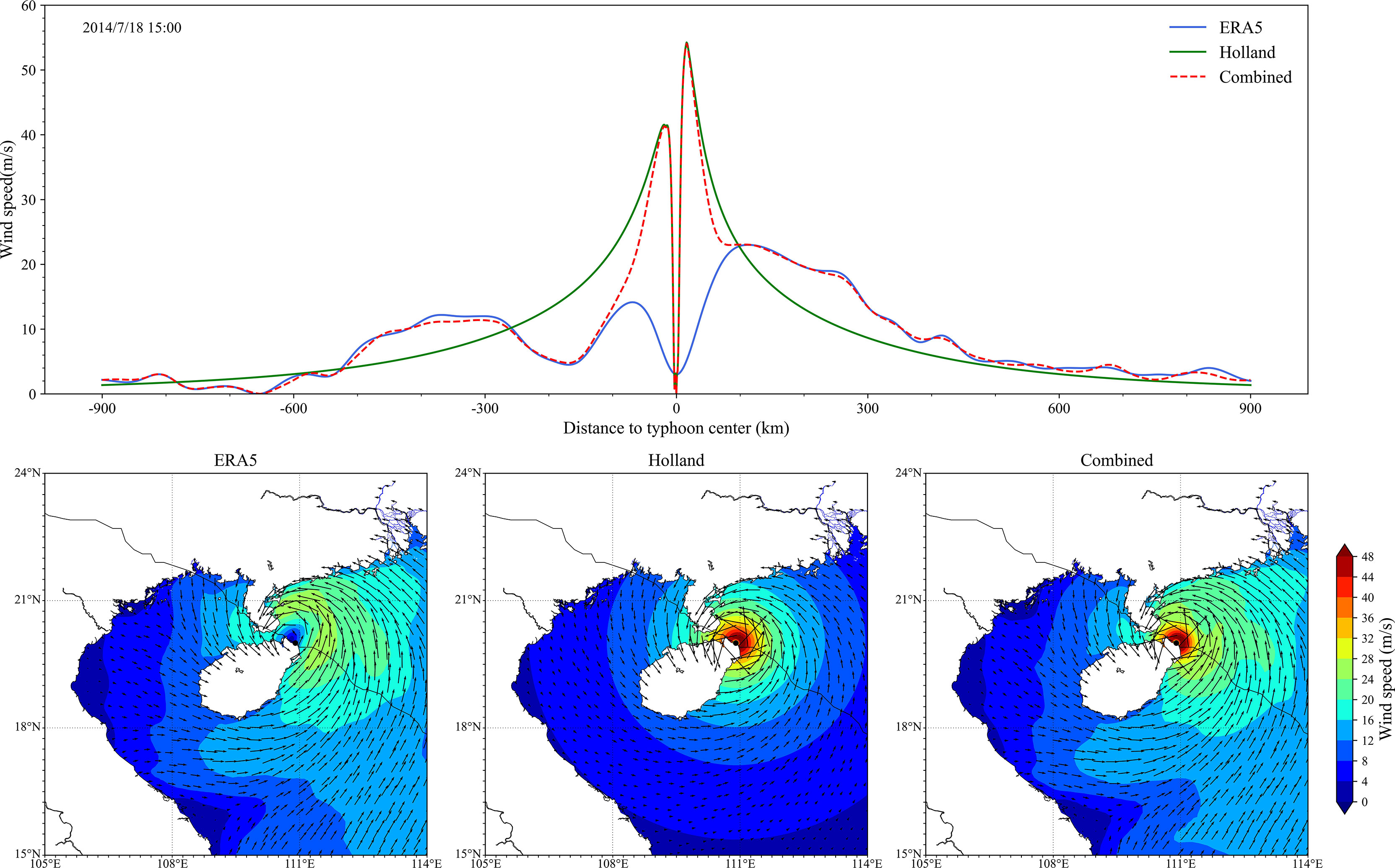
Figure 3 Wind speed profiles (upper panel) and spatial distributions (lower panel) from different wind fields. The location is shown in Figure 1.
In order to compare the performance of the SCHISM model under three different forcings, three tests (Tests 1–3) were carried out. In Test 1, the ERA5 pressure and Holland’s forcing wind fields were applied. In Test 2, we used the ERA5 data to execute the storm surge simulation. In Test 3, the reconstructed wind fields (see in Eqs. (23)–(25)) and the ERA5 pressure were assembled to drive the model. In this section, we ran 2-D simulations and compared storm surge hindcasts in three tests in the study area.
Figure 4 shows comparisons of observed and simulated storm surges at six tide gauge stations, and their PEs are given in Table 1. It can be seen that Test 3 gave a more accurate storm surge hindcast than the others. The simulation in Test 1 underestimated the peaks of storm surge and poorly modeled the surge forerunner caused by the remote wind at most stations. The result of Test 2 fit the observations better for the surge forerunner and its peak surges were also closer to the observed peak values than Test 1, except the Haikou station. The low-resolution reanalysis data (0.25°×0.25°) were unable to accurately reproduce wind speed at the cyclone center that led to the largest PE (−58.04%) at the Haikou station during Test 2. Test 3 had the lowest PEs in magnitude at all stations with the peak surges best matching observations; the combined wind field retained the advantages of both wind fields in Tests 1 and 2. Overall, the MAPEs (Table 1) show that the best performance is that of Test 3 (7.57%), the second is Test 2 (24.85%), and the worst is Test 1 (31.93%).
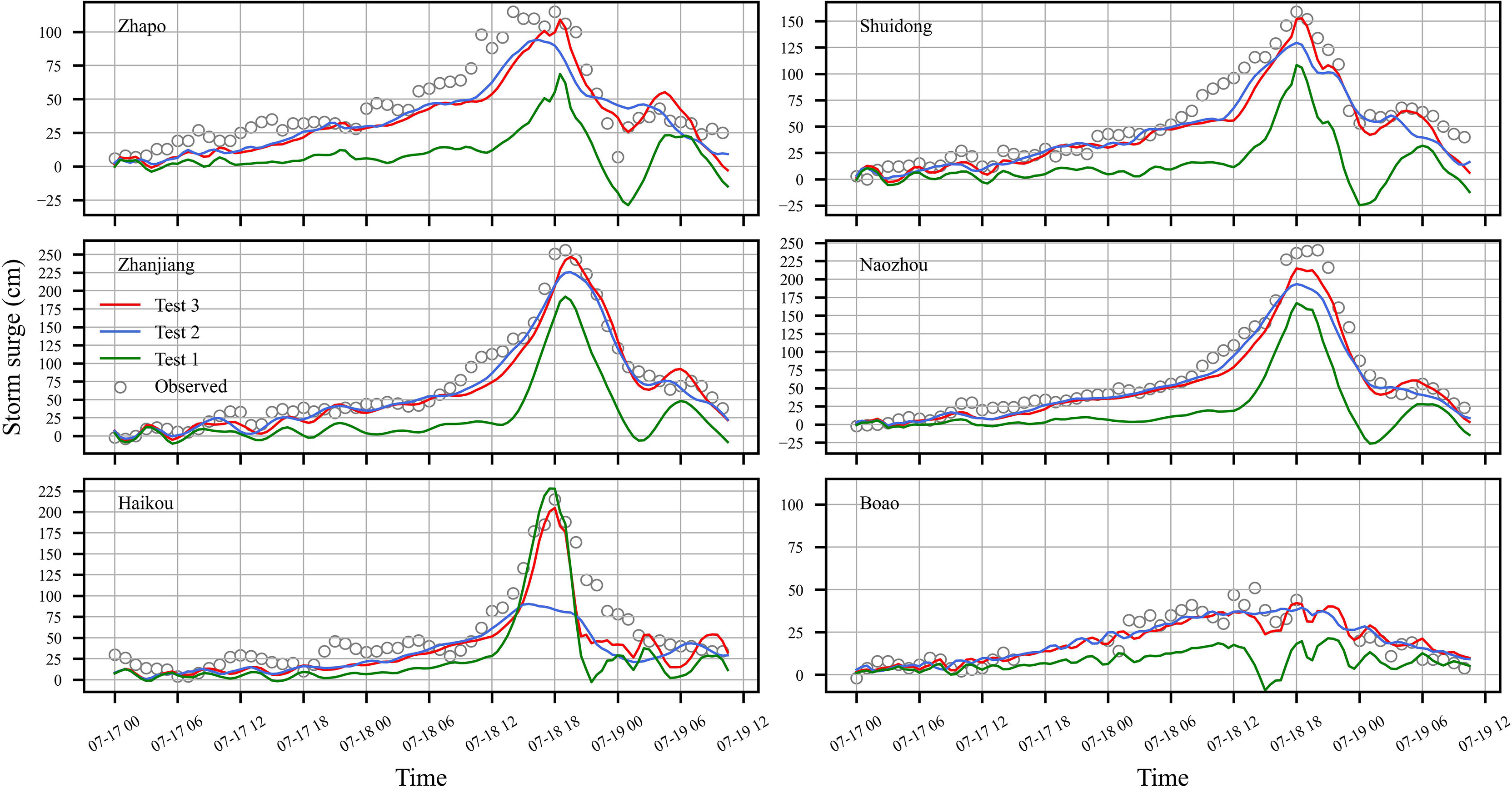
Figure 4 Time series of observed (circles) and simulated storm surges (cm) during Test 1 (green line), Test 2 (blue line), and Test 3 (red line) at six tide gauge stations.
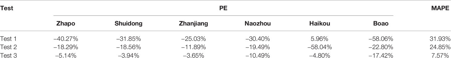
Table 1 PEs of peak surge between model simulation and observation under Tests 1–3.
To further evaluate model skill, statistical metrics (RMSE, Bias, and WS) about the time series of simulated and observed storm surge at all tide gauge stations were given (Figure 5). The three statistics show that the result of Test 3 performed best among the three tests. The averaged RMSE (15.9 cm) and Bias (−9.3 cm) values of Test 3 are smaller than results in Test 1 (41.9 cm and −33.8 cm) and Test 2 (17.9 cm and −10.3 cm). The averaged WS value (0.95) in Test 3 also indicated that it is more consistent with observation than Test 1 (0.71) and Test 2 (0.93). Overall, hindcast of storm surge under Test 3 shows the best agreement with observations among three tests. Thus, in the subsequent comparison of 3-D and 2-D models, we selected the ERA5 pressure and the combined wind field as the atmospheric forcings for the model.
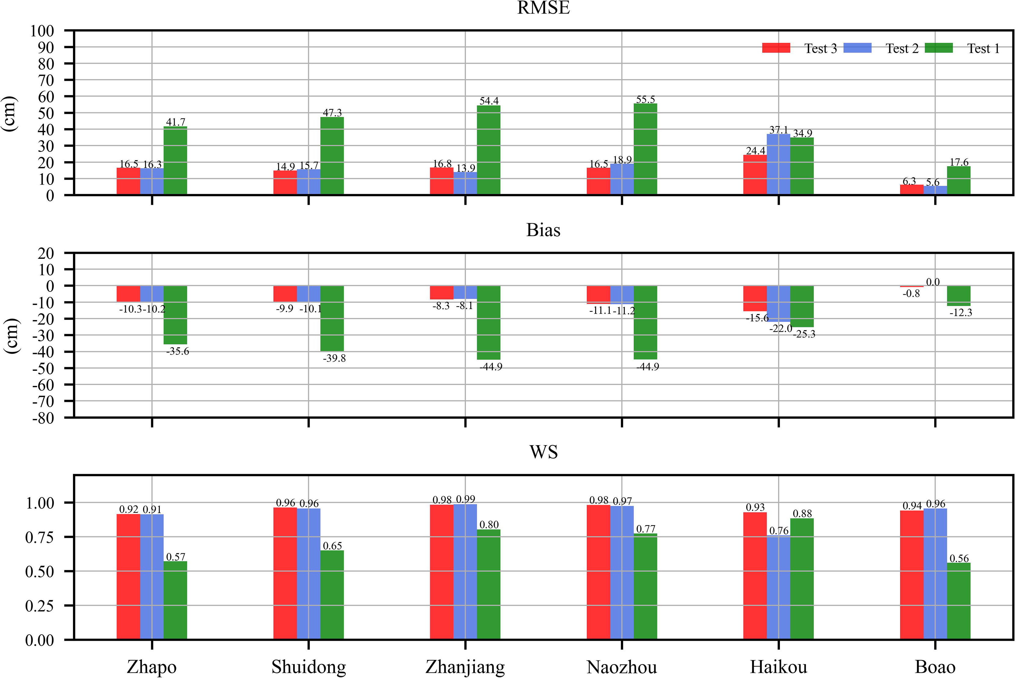
Figure 5 Statistical errors (RMSE and bias) and Willmott skill (WS) between observed and simulated storm surges heights (cm) under different tests at the six tide gauge stations.
In this section, the above statistical parameters were used to compare the performance of the 2-D (Test 4) and 3-D (Test 5) models. Figure 6 shows that although the simulation results of the 2-D and 3-D models are both in good agreement with the observed surges during typhoon Rammasun, there are some differences expected from the setup of both models. The time series of surges of the 2-D model at all stations were smaller than those of the 3-D model’s during the period. To clarify that, the PE and MAPE of the two tests were calculated to quantify the model reliability (Table 2). The 3-D model (4.22% MAPE) performed slightly better than the 2-D model (7.57% MAPE) overall. The PE values in Table 2 indicate that the 2-D model tended to underestimate the storm surges at most stations due to overestimation of bottom stress in the 2-D model (Weisberg and Zheng, 2008). The performances of the 3-D model at Zhapo, Zhanjiang, Naozhou, and Haikou stations (0.23%, 0.66%, −5.22%, and 0.13%) were better than the 2-D model (−5.14%, −3.65%, −10.49%, and −4.80%), while they were close at the remaining two stations. Overall, compared to the 2-D model, the peak predictions of the 3-D model had better quality, and their discrepancies between observation and simulation were considered acceptable.
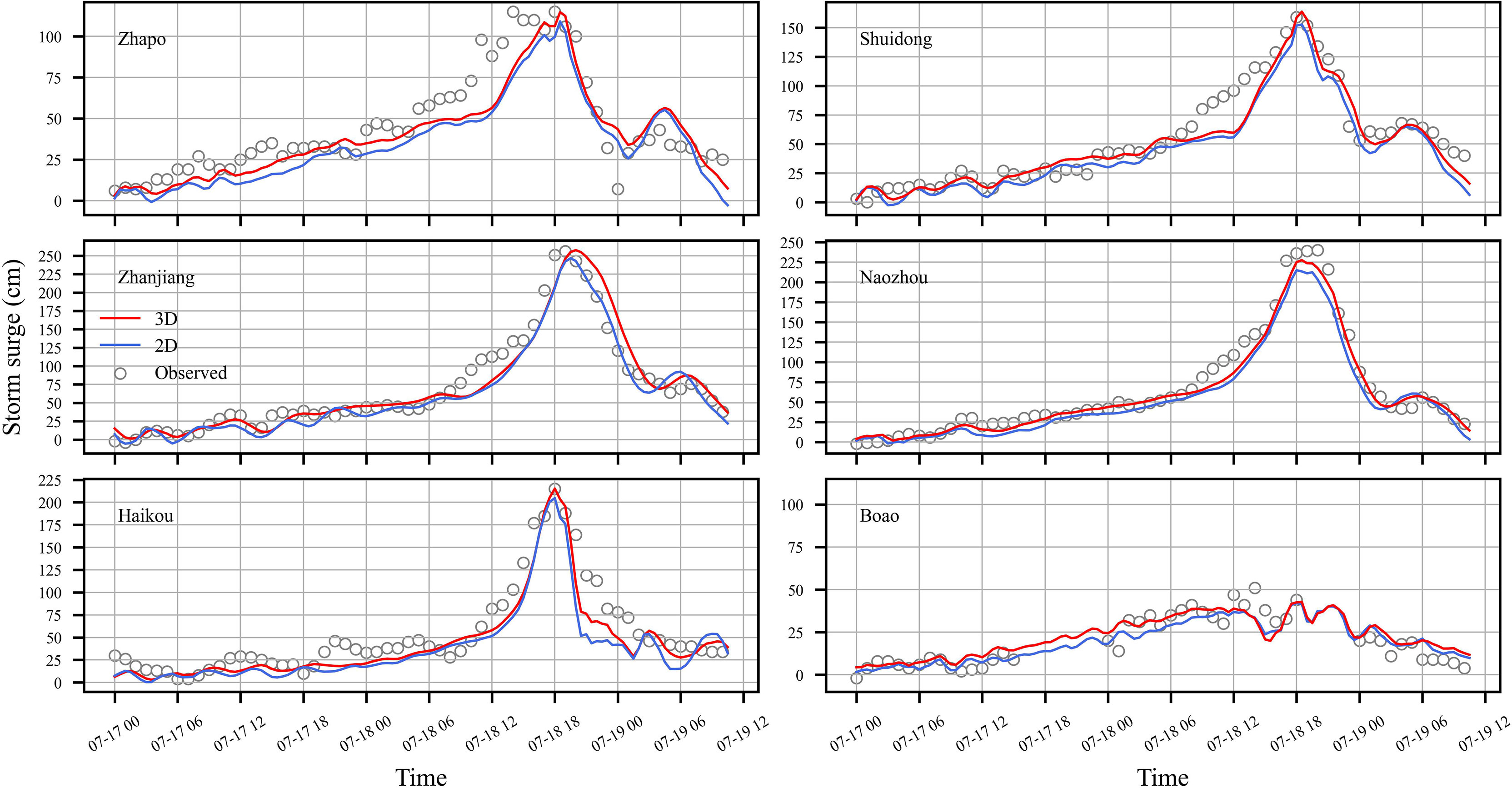
Figure 6 Time series of observed (circles) and simulated storm surges (cm) under the 2-D (blue line) and 3-D (red line) mode conditions at six tide gauge stations.

Table 2 PEs of peak surge between model simulation and observation under 3-D and 2-D models.
To further evaluate the performance of the two models, RMSE, Bias, and the WS values of both models were calculated and plotted in Figure 7. The average RMSE (13.4 cm) and average Bias (−3.8 cm) values of the 3-D model are smaller than results from the 2-D model (15.9 cm and −9.3 cm). Individually, the 3-D model has slightly lower accuracy than the 2-D model at Boao station. The WS values also demonstrated that the 3-D model (0.96) performed slightly better than the 2-D model (0.95) on average. From the above comparison, we can find that the 3-D SCHISM model reproduced the storm surges better than the 2-D model in the study area.
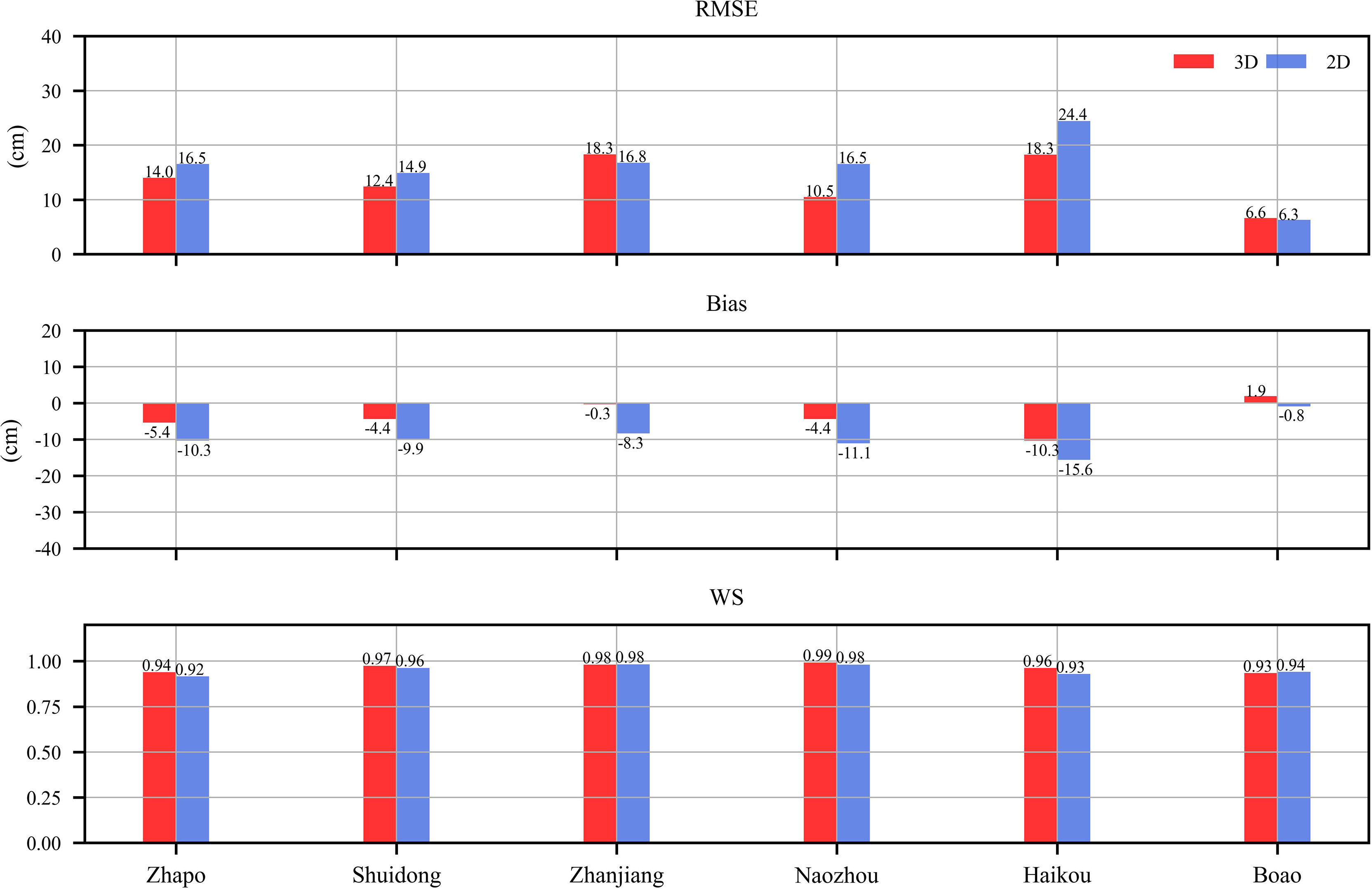
Figure 7 Statistical errors (RMSE and bias) and Willmott skill (WS) between observed and simulated storm surges heights (cm) under the 2-D (blue line) and 3-D (red line) mode conditions at six tide gauge stations.
The spatial discrepancies between 2-D and 3-D simulated peak surges are described in this section. We firstly plotted the spatial distribution of the peak surges under the 2-D condition (Figure 8A). The high storm surge mainly occurred along the eastern Leizhou Peninsula coast and offshore of the northeastern Hainan Island, with heights of >2 m. Offshore of the northeastern Hainan Island experienced especially severe water levels of about 3-m height due to being close to the track of typhoon Rammasun. In this region, it can be found that the 3-D model generates higher surges than the 2-D model, and the largest discrepancies between 2-D and 3-D simulated results were over 0.2 m (Figure 8B). Since the 2-D model generally underestimates the storm surges, the 3-D model is suggested as a better choice for surge simulation in the study area.
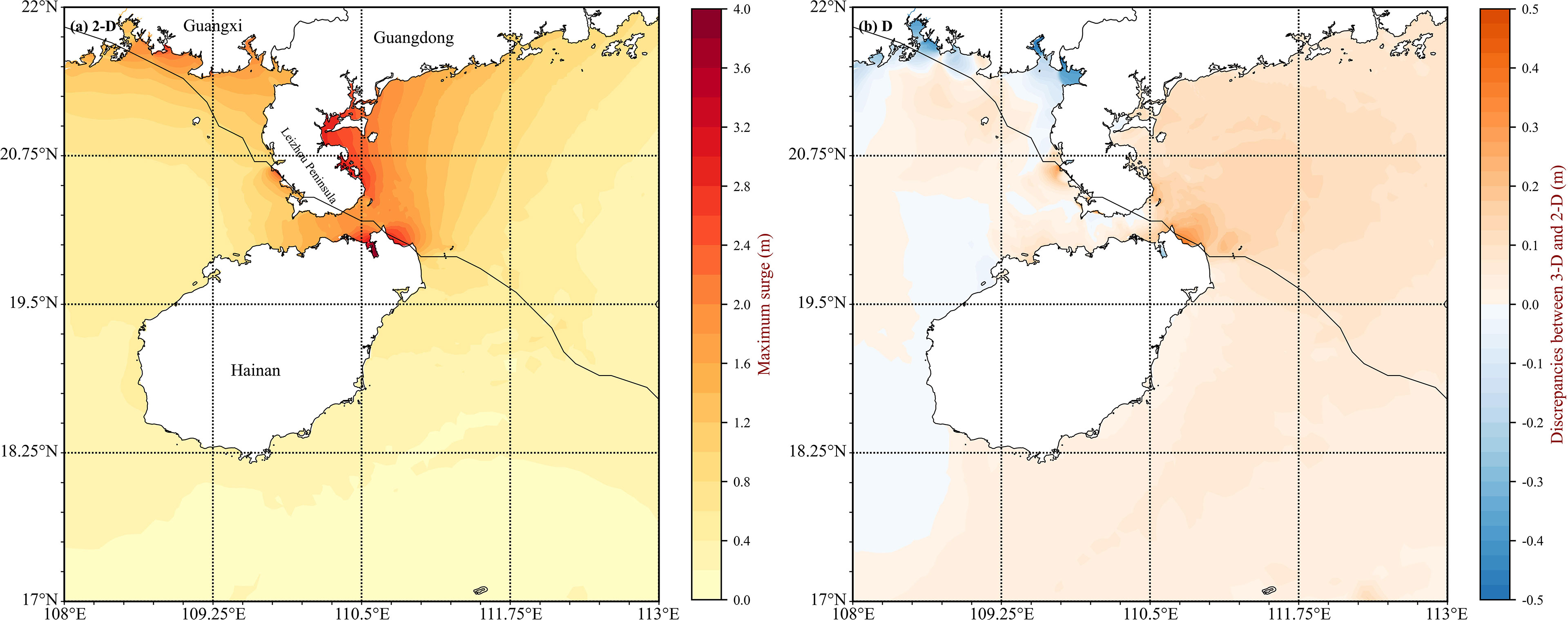
Figure 8 Spatial distributions of (A) peak surge (m) for the 2-D model and (B) the peak surge differences between the 3-D and 2-D models.
Four tests with different TC’s translation velocities are conducted in this study, named Tests 6–9 with 4, 2, 1/2, and 1/4 times initial moving velocity (Vmc), respectively. Figure 9 plots the discrepancies of peak surge heights between four tests and Test 5 (base case hereafter). When translation velocity was doubled, the changes of peak surge in most areas were insignificant except for the coastline of the western Guangdong Province in which peak surges increased from 0.1 to 0.5 m (Figure 9B). However, peak surges in most areas were lower than the initial scenario (extreme scenarios yield discrepancies of −1.6 m) when TC’s translation velocity was quadruple (Figure 9A). Halving the translation velocity produced lower peak surges (below −0.2 m) along the eastern Leizhou Peninsula coast (Figure 9C). Reducing translation velocity to a fourth, peak surges were slightly lower than the scenario with the 1/2 translation velocity (Figure 9D). Increased peak surges along the Guangxi Province may be caused by the terrain where sea water easily piled up in semienclosed bays. As the duration of the typhoon was longer, the phenomenon became more significant. For the region of complex terrain, due to the propagation speed of long waves below TC’s translation velocity, the typhoon wind cannot effectively affect the sea water redistribution to weaken storm surge heights. Conversely, when the typhoon has the lowest translation speed, higher surges occur in the semienclosed bay.
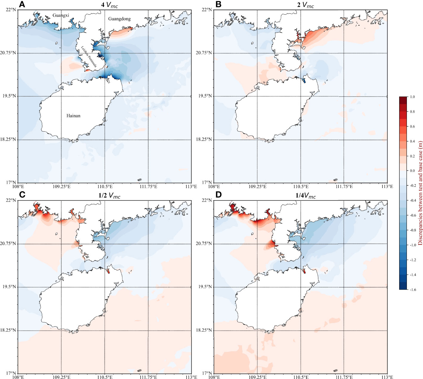
Figure 9 The discrepancies of peak surge heights between (A) Test 6 and Test 5, (B) Test 7 and Test 5, (C) Test 8 and Test 5, and (D) Test 9 and Test 6.
In most regions, the peak surge at Test 7 (doubled translation velocity with 30 mph) is the highest, and if we continue to increase or decrease translation velocity, the peak surge will decrease. When considering the spatial distribution of peak surges, the TC’s translation velocity moving across the shoreline is more likely to be the main factor for affecting surge heights. The relatively faster TCs within limits (Vmc ≤13.4 m/s) are more dangerous and cause higher surges.
To study the storm surge variations under different SLR scenarios once a similar typhoon approaches the study area, we used the above reconstructed atmospheric forcings and 3-D configurations as the basic model setup (Test 5). The non-uniform SLR values modify the original water depth of the model grid. Four future SLR conditions on years 2050, 2100, 2200, and 2300, respectively, were conducted (Tests 10–13) (Figure 2). We did not simulate the effect of flooding caused by storm surge or the change in the shoreline due to SLR. Therefore, the impact of coastal recession caused by storm surges is also beyond the scope of this study. We retained the same shoreline as the original scenario. To explore the spatial change of the peak surges (n) between the base case and experimental cases, their differences (Δn) in the study area were computed by:
where the subscript e stands for experimental case and c stands for the base case.
Figure 10 plots the Δn of four tests and shows that the peak surges in most coastal areas decreased with SLR. Near the TC’s track, the intensity of storm surges decreased significantly off the coast of the Leizhou Peninsula and offshore of the northeastern Hainan Island. In these shallow regions, interactions between surge and SLR became significant since the bottom friction and advective terms change nonlinearly with increase of the water depth (Zhang et al., 2013). The impact of SLR on surge was minor in open ocean where the interactions were relatively weak.
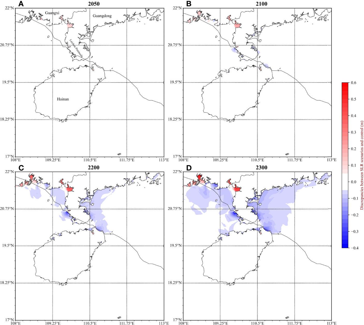
Figure 10 Spatial distributions of peak surge difference (m) between the base case (Test 5) and SLR scenarios (Tests 10-13) in year (A) 2050, (B) 2100, (C) 2200, and (D) 2300.
In shallow water, wind stress plays the most important role and the pressure gradient term in the momentum equation is unaffected by the water depths; thus, the 2-D mode of Eq. (3) could be simplified to a steady one-dimensional linearized equation where the free-surface elevation is only affected by wind stress and water depth (Park and Suh, 2012):
For one-dimensional space, ζ is the surface displacement caused by storm surges and x is the horizontal distance. H=h+SLR+ζ is the total water depth. τw=ρa·Cw·| U10 |·U10 is wind stress. τb=ρ·Cd·| ub |·ub represents the bottom stress. ub is the horizontal velocity in the 2-D model and the near-bottom velocity in the 3-D model. Further simplification leads to a better understanding of the correlation between storm surge and water depth:
L is the distance that the wind blows towards the shore on shelf. The storm surge amplitude (A) is proportional to the wind stress (τw) and is inversely proportional to total water depth (H). The 2-D model is a simplification of the 3-D model, and the actual storm surge is calculated in both models by using pressure gradient force to balance the boundary conditions (τw-τb); thus, the correlation between storm surge and water depth in the 3-D model is similar to the 2-D model. According to Eq. (28), storm surge is dependent on water depth and altered by rising sea levels in which increasing total water depth can reduce the maximum height of the storm surge under the same wind forcing. Thus, when wind speeds remained unchanged, the storm surges in the shallow water become lower with larger SLR. A similar impact of SLR on storm surge can be found in other coastal regions (Yang et al., 2014; Neumann et al., 2015; Chen and Liu, 2016).
To better explore the change of storm surge with SLR, we focused on the northeastern coast of Hainan Island where storm surge peaks change significantly with SLR. We selected a representative profile with five nodes (almost perpendicular to the coastline) to analyze how SLR alters storm surges in the study area (Figure 11A). It can be found that the rates of decrease of the maximum height at each node were almost linear with SLR and differed in that the surge height decreased faster with SLR at the node closer to the coastline (Figure 11B). The L of Eq. (28) at the coastal region is greater than that of the offshore and amplifies the effects of sea level change. These results indicate the stability of impact of SLR on reducing storm surges at the northeastern coast of Hainan Island. However, in contrast with the open coast, the peak surges were amplified at the semienclosed bays along the coast of Guangxi Province with future SLR (Figure 10). This trend is likely to be caused by the characteristics of the local terrain and typhoon track where the typhoon-induced water level first decreased and then sharply increased (Chen et al., 2016). During the flooding period, the open coast can supply more water to the bays as sea level rises and cause higher surges in the bays compared with the base scenario. In all cases, we used a fixed shoreline that may be another potential reason. The amplification of storm surge by SLR has also been found in other semienclosed bays with a fixed shoreline (Liu et al., 2018; Zhang et al., 2013).
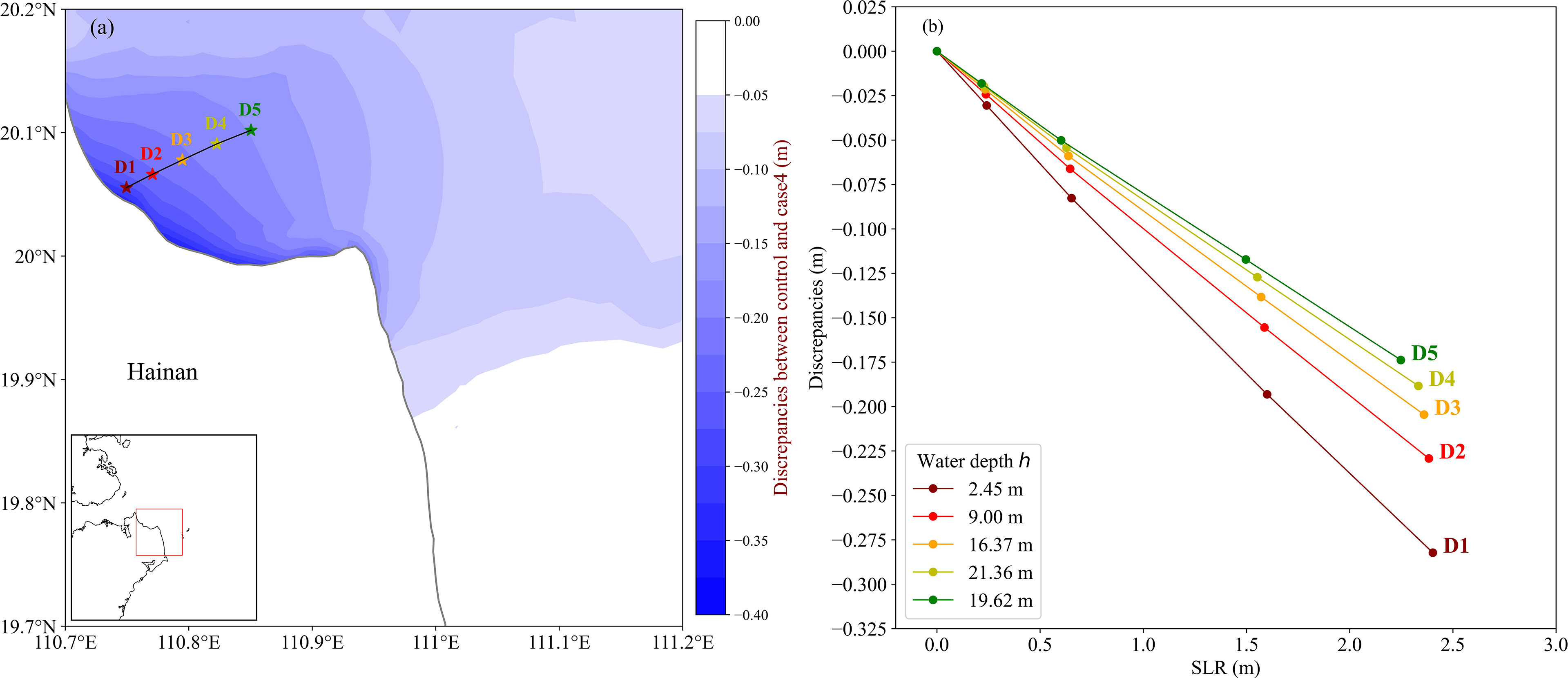
Figure 11 (A) Selected five representative nodes at the northeastern coast of Hainan Island. The background contour shows the peak surge difference (m) between the base case (Test 5) and SLR scenario in year 2300. (B) Peak surge differences between the base case and different SLR scenarios at the five nodes.
As consequences of global warming, sea level will continue to rise and more intense typhoons will be generated (Stowasser et al., 2007; Wu et al., 2014; Wu et al., 2022). Typhoon-induced storm surge superposed on SLR can bring severer hazards to coastal areas. In this study, the super typhoon Rammasun (2014) was selected as a case to reproduce typhoon-induced storm surge along the northwestern SCS using the SCHISM model. The impact of future SLR on local storm surge distribution was evaluated according to different SLR scenarios during the super typhoon period. To improve storm surge hindcasting skill by the numerical model in the study area, we simulated storm surge under different wind forcings and model schemes during the typhoon period. By comparing the results of different wind forcings in storm surge simulation, we found that the reconstructed wind between the Holland parametric model output and ERA5 reanalysis dataset based on a superposition method was the optimized option. The ERA5 reanalysis dataset was second to it. Under the same optimized wind forcing condition, the 3-D model has a better performance than the 2-D model for surge hindcast. The 2-D model underestimated peak surge significantly due to its overestimation of bottom drag based on a function of Manning coefficient. The TC’s translational velocity represents a large impact on the spatial distribution of peak surge. Within the propagation velocity of a long wave stimulated by TCs, the relatively faster TCs can easily generate higher surges.
Based on the 3-D model simulation, four SLR scenarios were considered from years 2050 to 2300. Model results demonstrated that increment in the water depth by SLR can alter spatial distribution characteristics of peak surges significantly, especially at the northeastern Hainan and Zhanjiang coastal areas with high surges. The peak surge decreased with SLR almost linearly in most regions due to the interaction between the storm surge and the SLR. Still, storm surge increased with SLR in many semienclosed bays along the Guangxi Province coast in which typhoon winds can drive more water into the semienclosed terrain and cause higher surges there.
The raw data supporting the conclusions of this article will be made available by the authors, without undue reservation.
YZ took part in running the model, writing the manuscript draft, and analyzing the results. ZN helped to design the model grid and storm surge model. PV helped to revise the manuscript and analyze the results. HX acted as PI supervisor in guiding the whole theoretic diagnoses and revised the manuscript. BH and HW revised the manuscript and gave pieces of advice on manuscript structure. WL and SL helped to collect and analyze the tide dataset. All authors contributed to the article and approved the submitted version.
This study is supported by the National Natural Science Foundation of China (grants 42176033 and 41976014), the CAS Frontier Basic Research Project (grant QYJC201910), the Strategic Priority Research Program of the CAS (grant XDA13030302), and the Youth Innovation Promotion Association CAS (grant 2022373).
The authors declare that the research was conducted in the absence of any commercial or financial relationships that could be construed as a potential conflict of interest.
All claims expressed in this article are solely those of the authors and do not necessarily represent those of their affiliated organizations, or those of the publisher, the editors and the reviewers. Any product that may be evaluated in this article, or claim that may be made by its manufacturer, is not guaranteed or endorsed by the publisher.
The Supplementary Material for this article can be found online at: https://www.frontiersin.org/articles/10.3389/fmars.2022.878301/full#supplementary-material
Akbar M. K., Kanjanda S., Musinguzi A. (2017). Effect of Bottom Friction, Wind Drag Coefficient, and Meteorological Forcing in Hindcast of Hurricane Rita Storm Surge Using SWAN. J. Mar. Sci. Eng. 5 (3), 38. doi: 10.3390/jmse5030038
Chen W. B., Liu W. C. (2016). Assessment of Storm Surge Inundation and Potential Hazard Maps for the Southern Coast of Taiwan. Nat. Haz. 82, 591–616. doi: 10.1007/s11069-016-2199-y
Chen B., Shi M. C., Chen X. Y., Ding Y., Zheng B. X., Dong D. X., et al. (2016). Water Level Fluctuations in Guangxi Near Coast Caused by Typhoons in South China Sea. Lop. C. Ser. Earth Env. 39. doi: 10.1088/1755-1315/39/1/012029
Dietrich J. C., Muhammad A., Curcic M., Fathi A., Dawson C. N., Chen S. S., et al. (2018). Sensitivity of Storm Surge Predictions to Atmospheric Forcing During Hurricane Isaac. J. Waterw. Port. Coast. 144 (1), 04017035. doi: 10.1061/(ASCE)WW.1943-5460.0000419
Ding Y., Ding T. D., Rusdin A., Zhang Y. X., Jia Y. F. (2020). Simulation and Prediction of Storm Surges and Waves Using a Fully Integrated Process Model and a Parametric Cyclonic Wind Model. J. Geophys. Res-Ocean. 125, e2019JC015793 . doi: 10.1029/2019JC015793
Drost E. J. F., Lowe R. J., Ivey G. N., Jones N. L., Pequignet C. A. (2017). The Effects of Tropical Cyclone Characteristics on the Surface Wave Fields in Australia’s North West Region. Cont. Shelf. Res. 139, 35–53. doi: 10.1016/j.csr.2017.03.006
Fox-Kemper B., Hewitt H. T., Xiao C., Aðalgeirsdóttir G., Drijfhout S. S., Edwards T. L., et al. (2021). “Ocean, Cryosphere and Sea Level Change,” in Climate Change 2021: The Physical Science Basis. Contribution of Working Group I to the Sixth Assessment Report of the Intergovernmental Panel on Climate Change. Eds. Masson-Delmotte V., Zhai P., Pirani A., Connors S. L., Péan C., Berger S., Caud N., Chen Y., Goldfarb L., Gomis M. I., Huang M., Leitzell K., Lonnoy E., Matthews J. B. R., Maycock T. K., Waterfield T., Yelekçi O., Yu R., Zhou B. (Cambridge University Press).
Gao Y., Wang H., Liu G. M., Sun X. Y., Fei X. Y., Wang P. T., et al. (2014). Risk Assessment of Tropical Storm Surges for Coastal Regions of China. J. Geophys. Res-Atmo. 119, 5364–5374. doi: 10.1002/2013JD021268
Garner G. G., Hermans T., Kopp R. E., Slangen A. B. A., Edwards T. L., Levermann A., et al. (2021) Ipcc Ar6 Sea-Level Rise Projections. Version 20210809. Po.Daac (CA, USA). Available at: https://podaac.jpl.nasa.gov/announcements/2021-08-09-Sea-level-projections-from-the-IPCC-6th-Assessment-Report (Accessed YYYY-MM-DD).
Garzon J. L., Ferreira C. M. (2016). Storm Surge Modeling in Large Estuaries: Sensitivity Analyses to Parameters and Physical Processes in the Chesapeake Bay. J. Mar. Sci. Eng. 4 (3), 45. doi: 10.3390/jmse4030045
Guillou N. (2014). Wave-Energy Dissipation by Bottom Friction in the English Channel. Ocean. Eng. 82, 42–51. doi: 10.1016/j.oceaneng.2014.02.029
Halpin E. (2006). Performance of the New Orleans Flood Protection System During Hurricane Katrina. International Journal on Hydropower & Dams 13, 41–49.
Holland G. J. (1980). An Analytic Model of the Wind and Pressure Profiles in Hurricanes. Monthly Weather Review 108 (8), 1212–1218. doi: 10.1175/1520-0493(1980)108<1212:AAMOTW>2.0.CO;2
Huang C. J., Qiao F. L. (2015). Sea Level Rise Projection in the South China Sea From CMIP5 Models. Acta Oceanol. Sin. 34, 31–41. doi: 10.1007/s13131-015-0631-x
Hu K. L., Chen Q., Kimball S. K. (2012). Consistency in Hurricane Surface Wind Forecasting: An Improved Parametric Model. Nat. Haz. 61, 1029–1050. doi: 10.1007/s11069-011-9960-z
IPCC. (2014). Climate Change 2014: Synthesis Report. Contribution of Working Groups I, II and III to the Fifth Assessment Report of the Intergovernmental Panel on Climate Change [Core Writing Team, Pachauri R.K., Meyer L.A. (eds.)]. IPCC, Geneva, Switzerland, 151 pp.
Jelesnianski C. P. (1972). SPLASH: (Special Program to List Amplitudes of Surges From Hurricanes). I, Landfall Storms. Available at: https://repository.library.noaa.gov/view/noaa/13509
Lapetina A., Sheng Y. P. (2015). Simulating Complex Storm Surge Dynamics: Three-Dimensionality, Vegetation Effect, and Onshore Sediment Transport. J. Geophys. Res-Ocean. 120, 7363–7380. doi: 10.1002/2015JC010824
Li A. L., Guan S. D., Mo D. X., Hou Y. J., Hong X., Liu Z. (2020). Modeling Wave Effects on Storm Surge From Different Typhoon Intensities and Sizes in the South China Sea. Estuar. Coast. Shelf. S, 235. doi: 10.1016/j.ecss.2019.106551
Lin N., Chavas D. (2012). On Hurricane Parametric Wind and Applications in Storm Surge Modeling. J. Geophys. Res-Atmo. 117, D09120. doi: 10.1029/2011JD017126
Liu X., Jiang W.S., Yang B., Baugh J. (2018). Numerical Study on Factors Influencing Typhoon-Induced Storm Surge Distribution in Zhanjiang Harbor. Estuarine Coastal and Shelf Science 215, 39–51. doi: 10.1016/j.ecss.2018.09.019
Lueck R. G., Lu Y. Y. (1997). The Logarithmic Layer in a Tidal Channel. Cont. Shelf. Res. 17, 1785–1801. doi: 10.1016/S0278-4343(97)00049-6
Mattocks C., Forbes C. (2008). A Real-Time, Event-Triggered Storm Surge Forecasting System for the State of North Carolina. Ocean. Model. 25, 95–119. doi: 10.1016/j.ocemod.2008.06.008
Neumann J. E., Emanuel K. A., Ravela S., Ludwig L. C., Verly C. (2015). Risks of Coastal Storm Surge and the Effect of Sea Level Rise in the Red River Delta, Vietnam. Sustainability-Basel 7, 6553–6572. doi: 10.3390/su7066553
Oppenheimer M., Glavovic B. C., Hinkel J., van de Wal R., Magnan A. K., Abd-Elgawad A., et al. (2019). “Sea Level Rise and Implications for Low-Lying Islands, Coasts and Communities,” in IPCC Special Report on the Ocean and Cryosphere in a Changing Climate. Eds. Pörtner H.-O., Roberts D. C., Masson-Delmotte V., Zhai P., Tignor M., Poloczanska E., Mintenbeck K., Alegría A., Nicolai M., Okem A., Petzold J., Rama B., Weyer N. M. (Cambridge, UK and New York, NY, USA: Cambridge University Press), 321–445. doi: 10.1017/9781009157964.006
Pan Y., Chen Y.-p., Li J.-x., Ding X.-l. (2016). Improvement of Wind Field Hindcasts for Tropical Cyclones. Water Sci. Eng. 9, 58–66. doi: 10.1016/j.wse.2016.02.002
Park Y. H., Suh K. D. (2012). Variations of Storm Surge Caused by Shallow Water Depths and Extreme Tidal Ranges. Ocean. Eng. 55, 44–51. doi: 10.1016/j.oceaneng.2012.07.032
Peng M. C., Xie L., Pietrafesa L. J. (2004). A Numerical Study of Storm Surge and Inundation in the Croatan-Albemarle-Pamlico Estuary System. Estuar. Coast. Shelf. S 59, 121–137. doi: 10.1016/j.ecss.2003.07.010
Pond S., Pickard G. L. (2013). Introductory Dynamical Oceanography, 2nd Edition (Oxford: Butterworth-Heinemann).
Rego J. L., Li C. Y. (2009). On the Importance of the Forward Speed of Hurricanes in Storm Surge Forecasting: A Numerical Study. Geophys. Res. Lett. 36, L07609. doi: 10.1029/2008GL036953
Shchepetkin A. F., McWilliams J. C. (2005). The Regional Oceanic Modeling System (ROMS): A Split-Explicit, Free-Surface, Topography-Following-Coordinate Oceanic Model. Ocean. Model. 9, 347–404. doi: 10.1016/j.ocemod.2004.08.002
Stowasser M., Wang Y. Q., Hamilton K. (2007). Tropical Cyclone Changes in the Western North Pacific in a Global Warming Scenario. J. Climate 20, 2378–2396. doi: 10.1175/JCLI4126.1
Ueno T. (1981). Numerical Computations of the Storm Surges in Tosa Bay. J. Oceanogr. Soc. Jap. 37, 61–73. doi: 10.1007/BF02072559
Weisberg R. H., Zheng L. Y. (2008). Hurricane Storm Surge Simulations Comparing Three-Dimensional With Two-Dimensional Formulations Based on an Ivan-Like Storm Over the Tampa Bay, Florida Region. J. Geophys. Res-Ocean. 113, C12001. doi: 10.1029/2008JC005115
Willmott C. J. (1984). “On the Evaluation of Model Performance in Physical Geography,” in Spatial Statistics and Models. Eds. Gaile G. L., Willmott ,. C. J. (Dordrecht: Springer Netherlands), 443–460.
Wu L., Chou C., Chen C. T., Huang R. H., Knutson T. R., Sirutis J. J., et al. (2014). Simulations of the Present and Late-Twenty-First-Century Western North Pacific Tropical Cyclone Activity Using a Regional Model. J. Climate 27, 3405–3424. doi: 10.1175/JCLI-D-12-00830.1
Wu L. G., Zhao H. K., Wang C., Cao J., Liang J. (2022). Understanding of the Effect of Climate Change on Tropical Cyclone Intensity: A Review. Adv. Atmo. Sci. 39, 205–221. doi: 10.1007/s00376-021-1026-x
Xu Y., Lin M. S., Zheng Q. A., Song Q. T., Ye X. M. (2016). A Study of Sea Level Variability and its Long-Term Trend in the South China Sea. Acta Oceanol. Sin. 35, 22–33. doi: 10.1007/s13131-016-0788-3
Xu H. Z., Zhang K. Q., Shen J. A., Li Y. P. (2010). Storm Surge Simulation Along the U.s. East and Gulf Coasts Using a Multi-Scale Numerical Model Approach. Ocean. Dynam. 60, 1597–1619. doi: 10.1007/s10236-010-0321-3
Yang Z. Q., Wang T. P., Leung R., Hibbard K., Janetos T., Kraucunas I., et al. (2014). A Modeling Study of Coastal Inundation Induced by Storm Surge, Sea-Level Rise, and Subsidence in the Gulf of Mexico. Nat. Haz. 71, 1771–1794. doi: 10.1007/s11069-013-0974-6
Yang J., Yan F. (2021). Storm Surges Influenced by Binary Typhoons of Saola and Damrey in 2012. Mar. Sci. Bull. 40 (2), 172–181. doi: 10.11840/j.issn.1001-6392.2021.02.006 (In Chinese)
Yang J., Yan F., Chen M. X. (2021). Effects of Sea Level Rise on Storm Surges in the South Yellow Sea: A Case Study of Typhoon Muifa, (2011). Cont. Shelf. Res. 215, 104346. doi: 10.1016/j.csr.2021.104346
Yang W. K., Yin B. S., Feng X. R., Yang D. Z., Gao G. D., Chen H. Y. (2019). The Effect of Nonlinear Factors on Tide-Surge Interaction: A Case Study of Typhoon Rammasun in Tieshan Bay, China. Estuar. Coast. Shelf. 219, 420–428. doi: 10.1016/j.ecss.2019.01.024
Zhang K. Q., Li Y. P., Liu H. Q., Xu H. Z., Shen J. (2013). Comparison of Three Methods for Estimating the Sea Level Rise Effect on Storm Surge Flooding. Clim. Change 118, 487–500. doi: 10.1007/s10584-012-0645-8
Zhang Y. L. J., Ye F., Stanev E. V., Grashorn S. (2016). Seamless Cross-Scale Modeling With SCHISM. Ocean. Model. 102, 64–81. doi: 10.1016/j.ocemod.2016.05.002
Keywords: storm surge, sea level rise, 2-D/3-D models, super typhoon Rammasun, the northwestern South China Sea
Citation: Zhou Y, Ni Z, Vetter PA, Xu H, Hong B, Wang H, Li W and Liu S (2022) Model Simulation of Storm Surge in the Northwestern South China Sea Under the Impact of Sea Level Rise: A Case Study of Super Typhoon Rammasun (2014). Front. Mar. Sci. 9:878301. doi: 10.3389/fmars.2022.878301
Received: 17 February 2022; Accepted: 20 May 2022;
Published: 21 June 2022.
Edited by:
Abiy S. Kebede, Brunel University London, United KingdomReviewed by:
Juan Manuel Sayol, University of Alicante, SpainCopyright © 2022 Zhou, Ni, Vetter, Xu, Hong, Wang, Li and Liu. This is an open-access article distributed under the terms of the Creative Commons Attribution License (CC BY). The use, distribution or reproduction in other forums is permitted, provided the original author(s) and the copyright owner(s) are credited and that the original publication in this journal is cited, in accordance with accepted academic practice. No use, distribution or reproduction is permitted which does not comply with these terms.
*Correspondence: Hongzhou Xu, aHp4dUBpZHNzZS5hYy5jbg==
Disclaimer: All claims expressed in this article are solely those of the authors and do not necessarily represent those of their affiliated organizations, or those of the publisher, the editors and the reviewers. Any product that may be evaluated in this article or claim that may be made by its manufacturer is not guaranteed or endorsed by the publisher.
Research integrity at Frontiers
Learn more about the work of our research integrity team to safeguard the quality of each article we publish.