Application of Airborne LiDAR Measurements to the Topographic Survey of the Tidal Flats of the Northern Jiangsu Radial Sand Ridges in the Southern Yellow Sea

The northern Jiangsu radial sand ridges are typical geomorphic deposit units distributed off the Jiangsu coast. A coastal tidal flat typically develops and provides a good habitat for many migratory birds and benthic organisms. However, topographic surveys of tidal flats have always been difficult in marine surveys because of the dense tidal creek, poor accessibility, and difficulty in setting up control points. In this study, we quickly obtained the point cloud data of the tidal flat near Yangkou Port in the southern part of the radial sand ridges based on an airborne LiDAR system, an integrated 3D laser scanner and a positioning and attitude determination system. We analyzed the adaptabilities of multiple filtering algorithms to tidal flats. In addition, a digital elevation model (DEM) of the tidal flat was constructed and the accuracy was verified with synchronized beach GPS-RTK topographic elevation measurements. The results show that the following: (1) Airborne LiDAR can quickly obtain high precision, high resolution, and a large area of ground point cloud information for tidal flats, overcoming the shortcomings of traditional measurement methods. (2) The triangulated irregular network (TIN) filtering effect is better than that of mathematical morphology and the filtering effect of point cloud normal vector clustering is mediocre. (3) The DEM of the LiDAR point cloud is in good agreement with RTK and the average error of the measurement results is 0.108 m. The error accuracy of the DEM satisfies the surveying specification of a 1:500 topographic map in a flat area, which proves that the airborne LiDAR system can be suitable for tidal flat elevation measurement. Nevertheless, it is possible to provide high precision terrain detection and DEM construction of a tidal flat with the development of airborne infrared and blue-green laser detection radar.

Introduction

Tidal flat refers to a muddy coastal intertidal shallow flat, which is the transition zone from land to sea and is located between the mean high tide and mean low tide (Wang and Zhu, 1990; Dyer et al., 2000). As the most important geomorphic component of coastal zones, tidal flats are widely distributed in many coastal zones around the world, including the coast of England, the coast of Wadden in Northern Europe, the banks of the Amazon in French Guiana, Gomso Bay in South Korea, and the coast of China (Mason et al., 1995; Wang, 2002; Ryu et al., 2008; Anthony et al., 2010; Loon-Steensma and Jantsje, 2015). At the same time, tidal flats are also the most sensitive land-sea dynamic interaction areas and have important ecological functions and social and economic values in protecting coastal areas from storm surges, increasing potential land resources, supporting biodiversity, and promoting carbon capture and storage (Murray et al., 2014; Zhang et al., 2017). However, tidal flats are facing serious threats and unprecedented challenges due to human activities, such as the construction of coastal ports and channels, reclamation, and natural factors such as sea level rise, storm surge, and biological invasion. Therefore, the observation of regular topographic changes in tidal flats is critical for coastal protection and sustainable development.

The scale of tidal flats is large in China, ranging from Liaoning in the north to Guangxi in the south, with a total tidal flat coastline length of 4000 km. In particular, the largest and widest tidal flat is distributed in the Jiangsu Province (Wang and Zhu, 1990; Xu et al., 2012). The northern Jiangsu radial sand ridges are typical geomorphic sedimentary units distributed off the coast of Jiangsu Province in China (Wang, 2002). Historically, the Yellow River delivered large amounts of sediment into the South Yellow Sea, especially in 1128-1855 AD, and the tidal flats of the radial sand ridges advanced seaward and formed the largest and most typical muddy coastal tidal flat in China, providing a favorable habitat for many migratory birds and benthic organisms (Zhang, 1984; Liu et al., 2013; Xu et al., 2018; Zhao et al., 2020). In recent decades, the topography of the coastal tidal flat in the radial sand ridges has changed significantly under the influence of sea level rise, global climate change, and human activities. However, the topographic surveys of the tidal flat in the radial sand ridges have always been difficult because of the tidal creek density, poor accessibility in data, and difficulty in setting up control points. At present, the main methods of topographic surveys for the silty tidal flat of the northern Jiangsu radial sand ridges are manual field surveys and remote sensing (Liu et al., 2004; Chen et al., 2010; Gong et al., 2014; Ding et al., 2014; Wang et al., 2018). However, field surveys are restricted because of low efficiency, high cost, limited measurement area of the tidal flat, and inadequate spatiotemporal coverage, although high precision can be obtained. Remote sensing methods for terrain monitoring mainly include the water boundary method and remote sensing water content method (Liu et al., 2012; Li and Gong, 2016; Kang et al., 2017; Li et al., 2018). Although large-scale monitoring can be obtained, there is a horizontal offset error in the calculation of shoreline spatial positioning, resulting in inaccuracy, which, in turn, cannot be used for large-scale mapping of a tidal flat. Oblique photography has a long data processing cycle and difficult image matching technology because of the limited number of image control points that can be arranged, the large amount of field work, and the monotonous texture information of a tidal flat. Airborne LiDAR measurement technology is an effective and innovative technology that integrates laser ranging technology, GPS differential technology, and inertial measurement unit (IMU) technology. As an active remote sensing technology, LiDAR is not limited by time and climate conditions, can provide all-weather observations of the Earth, and can quickly obtain high accuracy, high resolution digital terrain models, and three-dimensional coordinates of ground objects. In addition, LiDAR can also obtain the physical characteristics of the Earth’s surface, which cannot be accomplished using passive optical remote sensing. It provides a brand-new technical means for obtaining 3D geographic space information of a coastal zone with high accuracy, which has been widely applied for geological disasters, forests, agriculture, and glaciers (Krabill et al., 2000; Brock and Purkis, 2009; Zhao et al., 2018). Airborne LiDAR is currently the most accurate sensor technology and has a rapidly increasing application in intertidal zones. In recent years, airborne and unmanned aerial vehicle (UAV) platforms have been used in sandy coastal topography, coastal erosion, and marine mapping (Walker et al., 2013; David et al., 2015; Houser et al., 2015). At the same time, it is an efficient method to generate DEM (such unique, wide, gently sloping of tidal flat) in a short time. However, LiDAR technology is rarely used for topographic survey studies of muddy coastal tidal flats due to their gentle slope and shallow water.

In this study, we analyze the adaptability of multiple filtering algorithms in the tidal flat by implementing different filtering algorithms and interpolation algorithms. At the same time, constructing a digital elevation model (DEM) of a tidal flat and the verifying accuracy with synchronized beach GPS-RTK topographic elevation measurements. Our specific objectives were (1) to obtain original airborne LiDAR point cloud data and establish key technologies for generating a DEM of a tidal flat; (2) to discuss the adaptive range of the respective filtering algorithms of those technologies and analyze their advantages and disadvantages by implementing several mainstream filtering algorithms; and (3) to evaluate the influences of different data interpolation methods on DEM accuracy and compare their interpolation efficiency based on the results of the tidal flat control points.

Materials and Methods

Study Area

The northern Jiangsu radial sand ridges (NJRSRs) are located between the Sheyang River estuary and the Yangtze River estuary and cover an area of more than 200 km in length and 140 km in width, with a total area of 22,470 km² (Wang, 2012). The NJRSRs consist of more than 70 sand ridges and tidal channels ranging up to approximately 25 m in depth, with various dimensions radially centered on the coastal city of Jianggang. The current convergence and divergence between the radial sand ridges are affected by waves and regular semidiurnal tides (Xing et al., 2012). The sediment of the ridge system is composed of silt with median grain sizes ranging from 8~63 μm (Wang and Ke, 1997).

Rudong County is located in the central part of the coast of the NJRSRs, with a total coastline length of 102.59 km (muddy coast), and a sea area of approximately 4758 km² of which the tidal flat area is more than 60 km², accounting for 1/9 of the total tidal flat area of Jiangsu Province (Jin, 2018). In the offshore sea, sandbanks are scattered and alternate with waterways; there are the Jiangjiasha, Zhugensha, Taiyangsha, Huoxingsha channels and other sand ridges outside the northern coastline, and the Yaosha, Lengjiasha, Lanshayang, and Huangshayang channels are connected to the eastern coastline with good water depth and navigable conditions. The water depth in the offshore intertidal zone is shallow and the sediment grain size components are primarily composed of sand, silt, and clay, with an average grain size of 50.77~171.72 μm, and surface sediments are frequently affected by tidal currents (Huang et al., 2020). According to a 2005 and a 2015 comparative analysis of the measured topographic data of the intertidal tidal flats, the elevation distribution range of this area is between -6.5~1.9 m (1985 National elevation standard), and the net sedimentation volume is 3×10⁶ m³. The most obvious changes in erosion and deposition are concentrated between the ±1 m isobaths, accounting for 72.8% of the area of the survey area (Gu, 2018).

The monitoring area in this study is located on the muddy coast near Yangkou Port in Rudong County, Jiangsu Province (Figure 1). The impact of the tidal wave system formed after the confluence of the reflected tidal waves propagated from the Shandong Peninsula has formed a reciprocating current that converges and diverges with Jiang Port as the center (Zhu and Yan, 1998). Under the dynamics of convergent and divergent tidal currents, silty coastal tidal flats are typically developed. The tidal flat has a gentle slope and a large area, with an average width of 6.5 km of the tidal flat, especially in the Tiaozi mud tidal flat, which can reach 14 km. The tides are regular semidiurnal tides with an average tidal range of 2.5 m-4 m, and the measured maximum tidal range was 9.28 m (the largest tidal range recorded in coastal areas in China) in the Huangshayang channel (Ye et al., 1986). In addition, the Yangkou Port is the only port area in Nantong that has the prospect of a 200,000-ton berth construction with wide tidal flat resources and abundant land resources. In recent years, there has been frequent commercialization the Yangkou Port area, including fisheries and aquaculture, port industry, and maritime transportation. The monitoring area in this study is 10.5 km², near the Yangkou Port Lingang Industrial Park and the Yellow Sea Bridge (Figure 1).

FIGURE 1

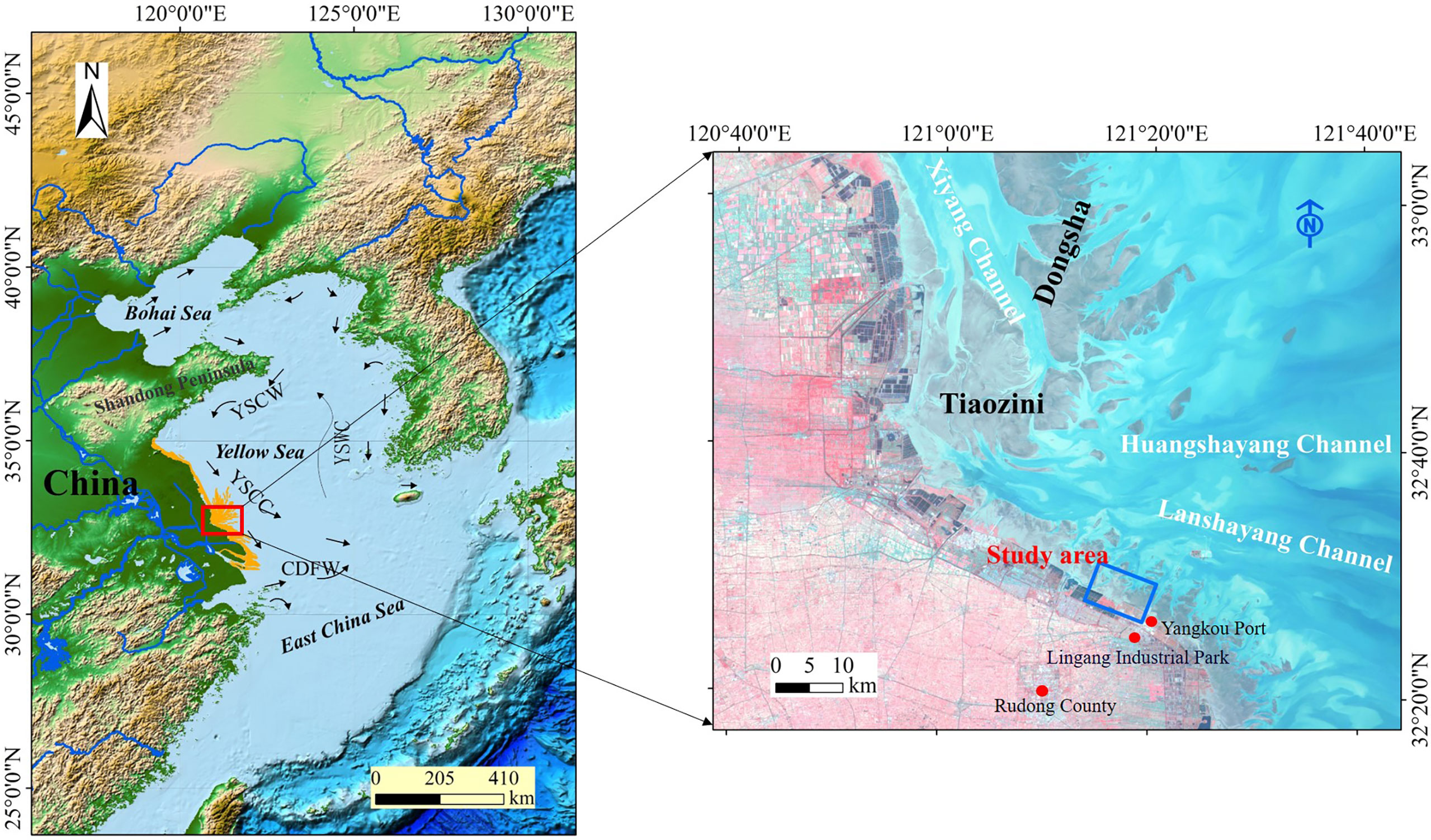
Figure 1 The map of study area.

LiDAR Monitoring System

The airborne LiDAR measurement site is located in the Lingang Industrial Park and its outer intertidal zone in Rudong County. The coastline of the measurement area is an artificial coastline, approximately 4 km long. The measurement range is approximately 2 km from the seawall to the sea, with an area of approximately 10.5 km² (Figure 1). Since the monitoring area is in the intertidal zone, it is submerged at high tide and exposed at low tide. Therefore, we chose to perform airborne LiDAR topographic surveys at low tides.

In this study, a light aircraft equipped with a laser scanning system was selected to obtain the original point cloud data. A total of 16 survey lines were laid out and the numbers of the survey lines were from L1 to L16 (Figure 2). The azimuth of the survey lines was determined to be near northwest to southeast and the flight direction angle was 33°~213°. At the same time, a GPS base station was set up in the survey area and its adjacent land area for synchronous observation to realize dynamic DGPS phase difference measurement and positioning. In addition, the 29 tidal flat survey points of tidal flat were measured based on GPS-RTK technology (Figure 2). The airborne laser scanning system selected for system is a Leica ALS70-HP Airborne LiDAR equipment, which mainly includes a LS70 laser scanner, SC70 control system box, RCD30 aerial camera, SPAN inertial navigation system, OC62 operation terminal, and other main components. The maximum scanning frequency is 200 Hz, the maximum pulse frequency is 500 kHz, the scanning angle is 45° or 60°, the maximum flight altitude is 3500 m and the minimum flight altitude is 200 m. After iterative processing of the calibration field point cloud result data, the mean square error of the checkpoint was less than 5 cm. The result system adopted WGS-84 and the elevation system adopted geodetic height system. The specific main technical parameters are shown in Table 1.

FIGURE 2

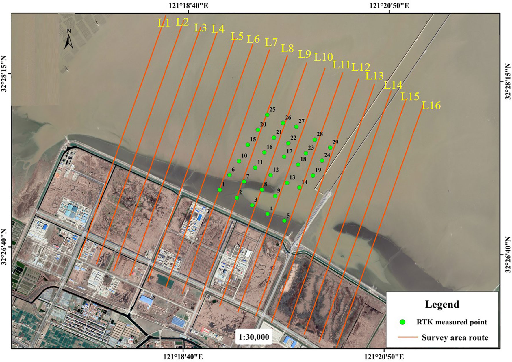
Figure 2 The Monitoring area and GPS-RTK station.

TABLE 1

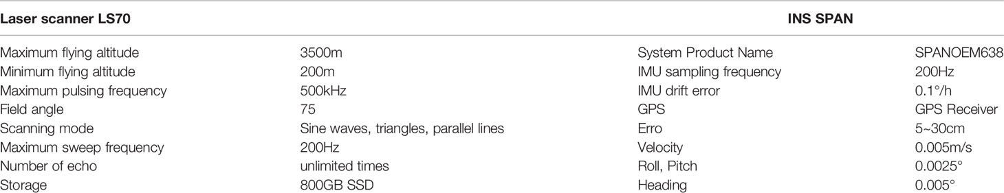
Table 1 Main technical parameters of Airborne LiDAR scanning system.

Ground Elevation Data Collection

To match the requirements of on-site measurement of tidal flats compared to assist aerial platform triangulation, a ground survey was carried out at the same time as the flight survey. TOPCON RTK (Hiper SR) was used in this study for the ground elevation survey. RTK is a measurement technology widely used in recent years because of its use of satellite positioning and the measurement accuracy of observation points is relatively higher, which is more convenient and rapid in tidal flats. The ground survey points were evenly arranged at an interval of approximately 300 m (Figure 2). The output result of the RTK elevation survey is in the data under the WGS 84 coordinate system and the elevation datum is the 1985 national elevation datum.

Measurement Methods of the Airborne LiDAR System

An airborne LiDAR laser scanning system integrates an optical mechanical scanner, laser rangefinder, differential GPS (DGPS) receiver, imaging equipment, inertial navigation system (INS), and a central control unit. An aircraft is used as the carrier to obtain three-dimensional coordinates on the ground to generate ground DEM products. An Airborne LiDAR system uses a laser scanning rangefinder emitted from the transmitter to the target, which is reflected back to the receiver by the target. There is a certain time difference during this period. By measuring the time difference, the rangefinder can accurately calculate the distance between the target and the launch center. The INS will measure the aircraft heading angle, roll angle, tilt angle, and other parameters during flight. In addition, the GPS system locates the position of the aircraft in real time and accurately calculates the specific coordinate information of the three-dimensional position of the laser point. The system principle is shown in Figure 3.

FIGURE 3

Figure 3 Schematic diagram of airborne LiDAR system.

Assuming a vector in three-dimensional space, the starting point coordinates O (X₀, Y₀, Z₀) can be measured, the radial path S from this point to a certain point Pi (X_i, Y_i, Z_i) on the ground is calculated, and the coordinates of point P can be determined through the joint vector calculation of the O coordinates. By accurately obtaining the position of the aircraft platform using GPS or DGPS, the coordinates of the projection center (X₀, Y₀, Z₀) can be determined. Then, a high precision attitude measurement INS is used to obtain the main optical axis attitude data (α, ω, k) at the projection center, and the angle θ between the observation direction and the normal is calculated. The three-dimensional coordinates of any specific point P on the ground can be determined (Sun et al., 2017).

$\begin{array}{ll}\{\begin{array}{l}{\text{X}}_{\text{i}}={\text{f}}_1\left({\text{X}}_0, {\text{Y}}_0, {\text{Z}}_0, \text{α}, \text{ω}, \text{k}, \text{S}, \text{θ}\right)\\ {\text{Y}}_i={\text{f}}_2\left({\text{X}}_0, {\text{Y}}_0, {\text{Z}}_0, \text{α}, \text{ω}, \text{k}, \text{S}, \text{θ}\right)\\ {\text{Z}}_{\text{i}}={\text{f}}_3\left({\text{X}}_0, {\text{Y}}_0, {\text{Z}}_0, \text{α}, \text{ω}, \text{k}, \text{S}, \text{θ}\right)\end{array}& (1)\end{array}$

Key Technologies of Point Cloud Data Processing

Airborne LiDAR data processing includes data preprocessing and postprocessing. Data preprocessing refers to solving the precise trajectory based on DGPS base station data and GPS and inertial navigation data, and finally generating the original laser point cloud data with the original laser scanning record. Data postprocessing is based on the original point cloud data, performing gross error elimination (including histogram analysis, outlier analysis, shaded relief map and profile map), data filtering (mathematical morphology, irregular triangulation, and point cloud normal vector) and human editors (including shaded relief map, profile map and aerial image). In addition, inverse distance weighted, kriging, and nature neighbor interpolation algorithm were selected to interpolate the filtered ground points and finally generating a DEM and other surveying and mapping products. The technical process of Airborne LiDAR data processing is shown in Figure 4.

FIGURE 4

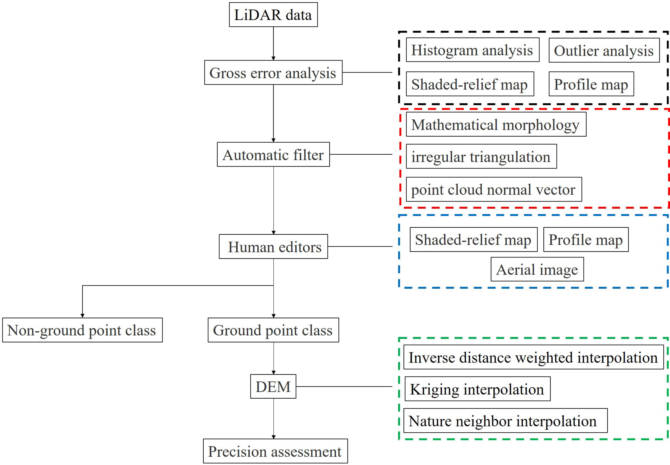
Figure 4 The flow chart of airborne LiDAR data processing.

To obtain the ground information of the laser point cloud more accurately, it is necessary to separate the ground points and nonground points from the point cloud data to retain the real ground point cloud and filter the ground object information and noise extracted from the point cloud (Brzank and Heipke, 2006). At present, the filtering methods of Airborne LiDAR point cloud data include filtering methods based on mathematical morphology (Sui et al., 2010), triangulation progressive encryption methods (Li et al., 2009), filtering algorithms based on slope, and filtering methods based on moving windows (Zhang, 2007). In this paper, a mathematical morphology filtering algorithm, triangulation iterative filtering algorithm, and point cloud vector clustering filtering algorithm are implemented to process relevant data in order to discuss the adaptability of several methods to intertidal tidal flats.

The mathematical morphology filtering algorithm includes basic algorithms such as the expansion operation, corrosion operation, opening operation, and closing operation and analyzes raster data by calculating the maximum, minimum, and average values of the data in the window (Chen, 2014). There are differences between point cloud data processing and image processing and the emphasis of morphological calculation is elevation rather than pixels. The irregular triangular net filtering algorithm assumes that the selected local area has a relatively flat terrain and the lowest point can be selected to replace the initial seed point in the grid. Then, a sparse triangulation network is constructed to comprehensively judge each point through the triangulation network. A schematic diagram of the triangulation filter is shown in Figure 5A.

FIGURE 5

Figure 5 (A) Schematic diagram of mathematical morphological filtering; (B) principle diagram of triangulation filter.

The irregular triangulation filtering method was formally proposed by Axelsson in the late 20th century (Axelsson, 2000). A point to be determined is represented by P and d represents the distance between the P and the projection surface. The angles between P and the vertices of the projection triangle (V1, V2, V3) are a, b, and c, and then determine the relationship between d, a, b, and c and a set threshold can be determined. If the result is within the threshold, P will be recognized as a ground point and TIN iteration will continue unless no new ground points are added (Figure 5B).

Where V1, V2, and V3 represent the vertices of the triangle, respectively. In the same plane, the expressions are as follows:

$\begin{array}{ll}{\text{A}}_{\text{x}}+{\text{B}}_{\text{y}}+{\text{C}}_{\text{z}}+\text{D}=0& (2)\end{array}$

where d represents the distance from P to the plane:

$\begin{array}{ll}\text{d}=\left|\frac{\text{A}{\text{x}}_{\text{p}}+\text{B}{\text{y}}_{\text{p}}+\text{C}{\text{z}}_{\text{p}}+\text{D}}{\sqrt{{\text{A}}^2+{\text{B}}^2+{\text{C}}^2}}\right|& (3)\end{array}$

S represents the distance from P to the three vertices V1, V2, and V3 of the triangle:

$\begin{array}{ll}{\text{S}}_{{\text{V}}_i\text{P}}=\sqrt{{\left({\text{X}}_{{\text{V}}_{\text{i}}}-{\text{X}}_{\text{p}}\right)}^2+{\left({\text{Y}}_{{\text{V}}_{\text{i}}}-{\text{Y}}_{\text{p}}\right)}^2+{\left({\text{Z}}_{{\text{V}}_{\text{i}}}-Z_{\text{p}}\right)}^2},\text{i}=1,2,3& (4)\end{array}$

and a represents the repetition angle:

$\begin{array}{ll}\text{a}=\text{arcsin}\frac{d}{{\text{S}}_{{\text{V}}_{\text{i}}\text{P}}}& (5)\end{array}$

In addition, a filtering algorithm of point cloud normal vector clustering was also used in this study. The upper and top surfaces of artificial ground objects such as bridges and roofs are relatively horizontal with gentle slopes and most of them are composed of several planes. The normal vectors of point clouds have similar characteristics and the normal vectors of any point are mostly distributed in one or more directions with strong regularity. The feature of a normal vector is affected by the spatial distribution of its neighborhood points. A normal vector is an important geometric characteristic in the point cloud data which can represent the trend of surface changes to a certain extent. With the fluctuation of the surface, the normal vector also changes accordingly. The basic method of point cloud normal vector clustering filtering is to select a seed point from the point cloud data and judge whether it meets the preset judgment standard by calculating the normal vector angle between the seed point and an adjacent point. If the neighboring points meet the criteria, they will belong to an area homogenous with the seed point until no new similar feature points are added in the neighborhood, so as to complete the segmentation of the ground feature point cloud and ground point cloud (Sun et al., 2019).

After the LiDAR data are filtered, there will be data holes in the ground point data. Thus, a data interpolation method can be used to eliminate data holes caused by filtering. The interpolation method is based on the continuous smoothness of the original terrain undulations and it is possible to interpolate the elevation of the neighboring data points to obtain the elevation of a pending point. We further discuss the practical application of three data interpolation methods: inverse distance weighting, kriging, and natural adjacent points in tidal flats.

Results and Discussion

In May 2019, airborne LiDAR measurements were carried out in the study area and measurements of 10.5 km² were obtained. The survey area covered approximately 1,650 m of coastline, extending approximately 1,500 m to land and 2,400 m to sea. A total of 2220.146 thousand point cloud data were obtained from aircraft scanning, with a density of 1.679 points/m², a maximum elevation value of 805.450 m, a minimum elevation value of -10.478 m, an average elevation value of 10.603 m, and an elevation standard deviation of 1.655 m (Figure 6).

FIGURE 6

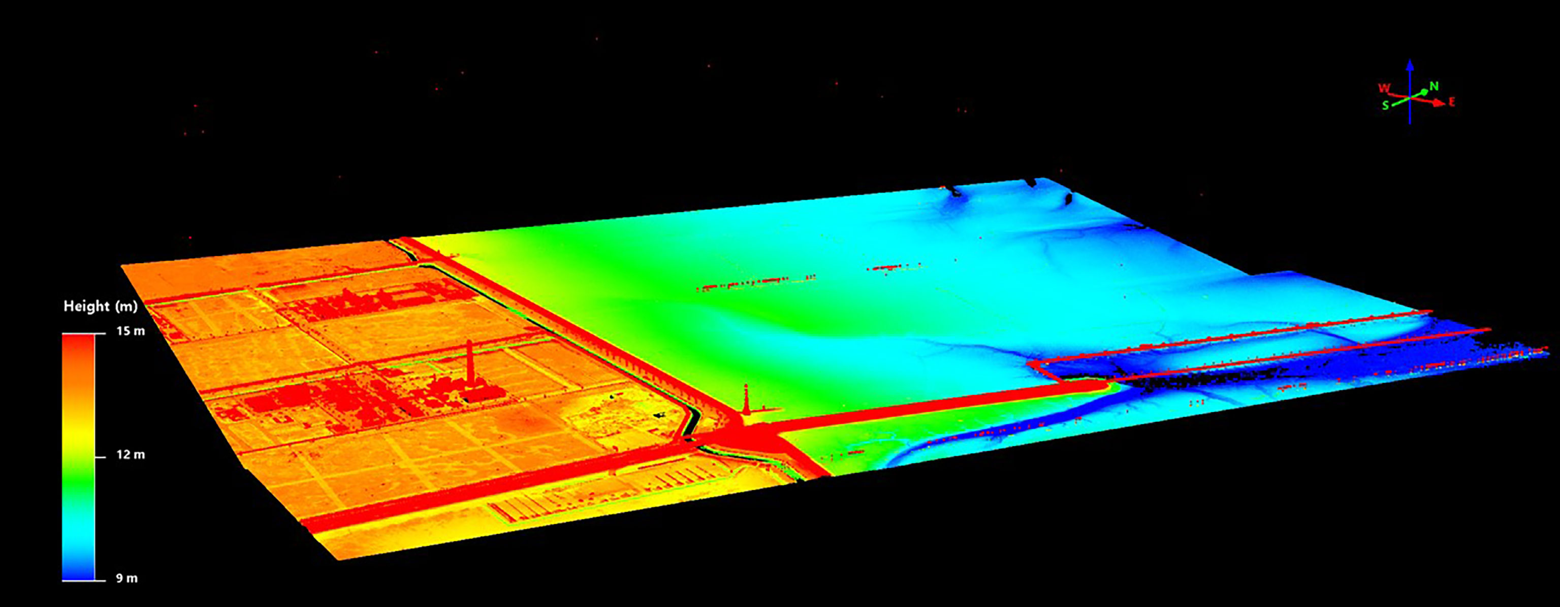
Figure 6 The results of point cloud data.

Gross Error Processing

When airborne LiDAR obtains point cloud data, it is highly random and vulnerable to interference from external factors and the scattering and diffraction of laser pulses. A considerable number of noise points (including high points, low points, and outliers) will inevitably appear (Wang, 2011; Zhang et al., 2012), which will affect the accuracy of the data and the construction of the DEM. The point cloud data need to be preprocessed before filtering and classification to eliminate noise points.

In this experiment, data interpolation was performed on the original point cloud data of the study region and to generate the point cloud shading map of the study area. However, it is difficult to eliminate noise points in the tidal flat area with this method. Gross error processing of outlier analysis uses Terrasolid software to eliminate the noise of the original point cloud data. The principle of this algorithm compares the elevation value of a point (the center point) with the elevation value of each point within a given distance. If the center point is significantly lower than the other points, the point will be separated. The set parameter excludes points within 5 m from the points that are lower than the general ground height of 0.5 m. The set parameters exclude points at a radius of 5 m and a high-level error greater than 5 times the standard deviation. The set parameter excludes points within 5m from the point 0.5m below the general ground height, and the radius of parameter elimination is the point with high error greater than 5 times standard deviation within 5m.

According to the profile of the original point cloud data of the study area (Figure 7A), it can be found that there is no special regularity in the distribution of gross error points and the number of points around gross error points is relatively small. After analysis, the elevation range of extremely high points is between 168.060 and 805.450 m, and the range of the extremely low points is between -10.478 and 9 m (Figure 7B), which provides a certain reference for establishing the histogram gross error analysis threshold.

FIGURE 7

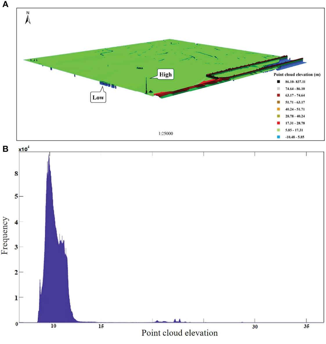
Figure 7 (A) the original point cloud data profile; (B) the original point cloud data elevation statistical histogram.

The abscissa of the point cloud elevation histogram represents the elevation value of the point cloud and the ordinate represents the frequency of occurrence of the elevation value. The number of points with a statistical elevation value less than 8.6 m or greater than 35 m is extremely small and the frequency of normalized elevation values within this range is less than 15 m. Therefore, 35 m is taken as the high point threshold and elevation values greater than this value are eliminated; 8.6 m is taken as the low point threshold and elevation values lower than this value are eliminated. The eliminated gross error points are superimposed with the remote sensing image to further clearly and intuitively analyze the source and distribution of gross error points.

In this experiment, a total of 538 gross error points were eliminated through the outlier analysis, point cloud profile, and elevation statistical histogram, including 354 extremely low points and 184 extremely high points (Figure 8). The elevation values of the extremely low points are -10.48~1.47 m and the average elevation value is -2.53 m. The elevation values of the extremely high points are between 36.32 m and 805.45 m and the average elevation value is 92.32m. The extremely low points in the survey area are concentrated and distributed in strips on the east and west sides of the Yellow Sea Bridge and these points do not belong to the surface points, as most of them come from systematic errors. These extremely low points are significantly lower than the tidal flat points because the emitted laser pulses are reflected back to the receiving device multiple times by the tidal flat surface. However, the number of extremely high points in the survey area is small and the distribution is disorderly and without obvious regularity. In addition, the extremely high points are not ground points and usually come from aerial objects such as birds and low-altitude aircraft. Consequently, there is an obvious height difference between the gross error points, the tidal flat terrain, bridges, and other ground objects. The gross error points can be effectively eliminated through the statistical histogram of the point cloud elevation. The point cloud data, after the gross error is eliminated, is further processed through a specific filtering algorithm.

FIGURE 8

Figure 8 (A) The removed gross error points; (B) The denoised point cloud data.

Filtering Processing

The three filtering methods proposed above are used to perform filtering experiments on the point cloud data after eliminating the gross errors points. The ground points obtained through mathematical morphology filtering, irregular grid TIN filtering, and point cloud normal vector filtering are shown in Figure 9.

FIGURE 9

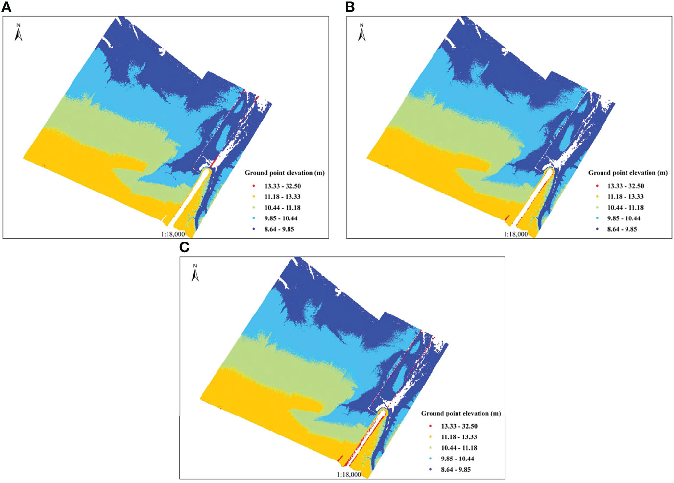
Figure 9 The results of Mathematical morphology filtering (ground points) (A); Irregular Triangulation filtering (B); Point cloud normal vector filtering (C).

On this basis, the laser footprint error rate specified by ISPRS is used as an evaluation criterion and it is combined with the actual situation divided into three types of errors to qualitatively evaluate the filtering effect of the three filtering algorithms, e.g., type I error (a ground point error is classified as a nonground point error), type II error (a nonground point is regarded as a ground point error), and total error (Hu et al., 2015). The specific calculation formula is shown in Table 2, where ‘a’ represents the number of ground points correctly classified, ‘b’ represents the number of ground points that are incorrectly divided into nonground points, ‘c’ represents the number of nonground points incorrectly divided into ground points, ‘d’ represents the number of nonground points correctly classified, and ‘n’ represents the total number of laser points.

TABLE 2

Table 2 Error calculation formula.

Artificial classification was carried out according to the point cloud profile of the study area and aerial photography assisted interpretation, and after filtering by the three algorithms, the type I error, type II error, and total error were calculated respectively (Table 3) since there are no standard reference point cloud data in the study area. The purpose of filtering is to restore the real terrain and the number of nonground points and after filtering, the number should be reduced, e.g., the type II error should be minimized.

TABLE 3

Table 3 Accuracy analysis of filtering results.

The type I error of the mathematical morphology filtering method is 0.19%, which is higher than that of the other two algorithms. This kind of error is mostly concentrated on the edges of buildings such as pipe racks and bridges and has relatively obvious terrain fluctuation and results in misclassification. The design principle of the algorithm in this paper is to classify ground points as ground object points as much as possible, so some ground points will be misclassified into ground object points, but such misclassified points have little influence on the subsequent interpolated DEM data in the later period. The key to this algorithm is the setting of the window size. However, there are relatively few ground objects in the tidal flat, so a large number of ground points can be saved and most ground points can be eliminated under the premise of setting an appropriate window size. The data organization form of this algorithm is a regular grid, which reduces the accuracy of the original data and increases the difficulty of filtering.

The type II error and total error distributions of the point cloud normal vector clustering filtering method are 3.98% and 0.32%, respectively, and the filtering effect is relatively poor, which indicates that the algorithm’s ability to filter ground objects needs further improvement. The principle of the algorithm is that the normal vector of the point cloud is similar to that of a ground point cloud with a flat roof surface or small curved surface, but the normal vector characteristic of a point depends on the spatial distribution of the surrounding points. For the point cloud data at the boundary of buildings with complex top structures and tall buildings, the algorithm cannot completely filter out the ground objects, and the filtering effect will be especially poor at relatively low point cloud densities. A small part of the tidal flats was flooded around the bridge and the laser points were lost. Thus, the point cloud density is low and the filtering effect is general. In addition, the filtering accuracy of the algorithm is also affected by the determination of neighborhood point sets. The point cloud data of the study area include ground objects with relatively complex top structures, such as pipe racks and electric towers. The point cloud density in some tidal flats is low and lacks prior knowledge of filtering, so the algorithm has certain limitations in tidal flats, resulting in high numbers of type II error and total errors.

The type II error and total error of the irregular triangulation filter method are relatively low, 2.84% and 0.18%, respectively. Under the premise of an appropriate threshold setting, the filtering ability for complex buildings and their surrounding microfeatures is slightly better than that of other two algorithms. The advantage of this algorithm is that the original point cloud data will not be lost and the terrain information can be better preserved. The disadvantage of this algorithm is that it must have prior knowledge of the largest building size and slope in the survey area. If the initial ground point selection effect is not satisfactory, the filtering accuracy will be greatly reduced. In addition, the algorithm needs to be continuously encrypted, which requires a long processing time. The filtering results of the irregular triangulation network filtering algorithm show that the removal effect of this method on different ground objects is considerable (Figure 6). Buildings (houses and oil tanks) with large areas and simple structures are well removed. In addition, the higher vegetation (mainly located on both sides of a road) is better filtered because it changes significantly compared to the surrounding terrain. Consequently, the algorithm can better separate obvious ground features.

Construction and Accuracy Verification of the Tidal Flat 3D DEM

After denoising and filtering out the generated laser point cloud data, inverse distance weighted interpolation, kriging interpolation, and the natural neighbor interpolation method based on ArcGIS 10.3 software was used to interpolate the real ground point cloud data of the tidal flat to generate a tidal flat DEM (Figure 10). At the same time, five vertical coastal sections were established and the topographic profile was measured using GPS-RTK while the airborne LiDAR system collected the muddy coastal topographic data. The accuracy of the DEM results generated by the airborne LiDAR point cloud is verified based on the synchronized GPS-RTK elevation data (Table 4). The section extracted from the point cloud generation DEM obtained using LiDAR is in good agreement with the section point data measured using RTK and shows a consistent trend of change. However, there are large errors in individual points mainly due to the high humidity on the tidal flat or the presence of water. The laser cannot penetrate the water, which has an impact on the accuracy.

FIGURE 10

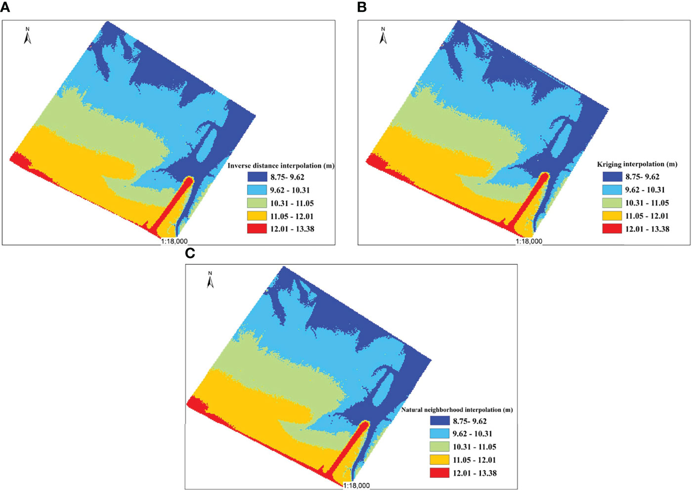
Figure 10 DEM shading map of tidal flat. (A) Inverse distance interpolation; (B) Kriging interpolation; and (C) Natural neighborhood interpolation.

TABLE 4

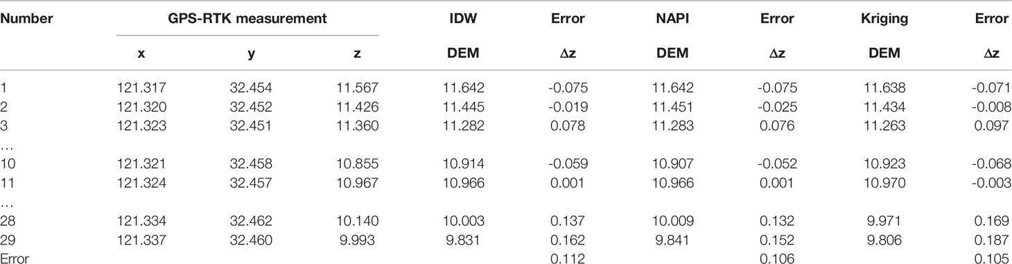
Table 4 The accuracy evaluation of DEM.

Through the analysis of the experimental results of the above three data interpolation methods, the filtered tidal flat point cloud data has no gross error points and no abnormal elevation values. The DEM shading effect map generated by the three interpolation methods of inverse distance weighting, kriging, and natural adjacent points has similar results: good smoothness, strong continuity, and has good interpolation results for the area with missing data. Consequently, the mean square error of DEM elevation processed by inverse distance weighting, natural adjacent points, and Kriging interpolation are 0.112 m, 0.106 m and 0.105 m, respectively, by using two measurement methods to subtract the obtained elevation values (Table 4). The average value of the error in the elevation is 0.108 m and the accuracy of the error in the elevation meets the 1:500 topographic map measurement specification for flat areas, indicating that the airborne LiDAR system can be suitable for tidal flat elevation measurement at low tide levels. In addition, the interpolation accuracy of natural adjacent points is equivalent to that of Kriging interpolation in terms of the accuracy of tidal flat DEM, which is higher than that of inverse distance weighted interpolation, but the kriging method has the lowest processing efficiency and takes too long. Therefore, considering the factors of processing efficiency and accuracy, it is recommended to use natural adjacent points for interpolation in the production of tidal flat DEM.

Conclusion

In this paper, the LiDAR point cloud data were collected in the Yangkou Port area of Rudong County in Jiangsu Province and the key technology of airborne LiDAR point cloud data postprocessing of typical intertidal tidal flats in Jiangsu were discussed. The airborne LiDAR point cloud data process was designed to quickly generate a high precision tidal flat DEM. The accuracy of tidal flat check points measured in the field was verified using GPS-RTK technology. The results show the following:

1. Airborne LiDAR, as an active remote sensing technology, can quickly obtain high precision, high resolution, and a large area of the ground object parameter information, providing new technical means for the high precision and fast acquisition of three-dimensional tidal flat geographic space information, overcoming the shortcomings of traditional measurement methods.

2. In the process of filtering, mathematical morphology, irregular grid TIN, and point cloud normal vector clustering have better filtering effects for most flat and sparse tidal flats. In general, the TIN filtering effect is better, followed by mathematical morphology, and the point cloud vector clustering filtering effect is general. If we have a priori knowledge of the topography and features in the survey area, the filtering accuracy will be greatly improved;

3. Based on an airborne LiDAR system with an integrated 3D laser scanner, positioning and attitude system, tidal flat point cloud data can be quickly acquired, a DEM generated, and its accuracy verified with synchronized tidal flat GPS-RTK terrain elevation measurements. The section extracted from the point cloud-generated DEM obtained using LiDAR is in good agreement with the section point data measured by RTK, which shows a consistent change trend. The average error of the measurement results is 0.108 m, and the accuracy of the errors in the elevation meets the 1:500 topographic map measurement specifications for tidal flat. The expected results have been achieved, which further shows that an airborne LiDAR system can be well adapted to the needs of tidal flat elevation measurement at low tide levels.

4. The LiDAR measurements have null values in tidal flat ponding, which will affect the accuracy of the tidal flat topography. The development of airborne infrared and blue-green laser detection radars provide the possibility for high precision terrain detection and DEM construction in the water areas of a tidal flat.

Data Availability Statement

The raw data supporting the conclusions of this article will be made available by the authors, without undue reservation.

Author Contributions

HZ: writing—original draft preparation. LW, JC, and HZ: collection and analysis of the data and software. YZ: investigation and validation. YZ and MX: conceptualization, funding acquisition, and project administration. YZ and MX: supervision. All authors contributed to the article and approved the submitted version.

Funding

This research was funded by the Marine Science and Technology Innovation Project of Jiangsu Province (No. JSZRHYKJ202002, HY2018-03, JSZRHYKJ202103), and the Nanjing Science and Technology Innovation Project for Overseas Students (1614100001).

Conflict of Interest

The authors declare that the research was conducted in the absence of any commercial or financial relationships that could be construed as a potential conflict of interest.

Publisher’s Note

All claims expressed in this article are solely those of the authors and do not necessarily represent those of their affiliated organizations, or those of the publisher, the editors and the reviewers. Any product that may be evaluated in this article, or claim that may be made by its manufacturer, is not guaranteed or endorsed by the publisher.

Acknowledgments

The authors would like to thank the reviewers for their valuable comments for the improvement of the manuscript.

References

Anthony E. J., Gardel A., Gratiot N., Proisy C., Allison M. A., Dolique F., et al. (2010). The Amazon-Influenced Muddy Coast of South America: A Review of Mud-Bank–Shoreline Interactions. Earth-Sci. Rev. 103, 99–121. doi: 10.1016/j.earscirev.2010.09.008

CrossRef Full Text | Google Scholar

Axelsson P. (2000). DEM Generation From Laser Scanner Data Using Adaptive TIN Models. Int. Arch. Photogramm. Remote Sens. 33, 110–117.

Google Scholar

Brock J. C., Purkis S. J. (2009). The Emerging Role of Lidar Remote Sensing in Coastal Research and Resource Management. J. Coast. Res. SI (53), 1–5. doi: 10.2112/SI53-001.1

CrossRef Full Text | Google Scholar

Brzank A., Heipke C. (2006). Classification of Lidar Data Into Water and Land Points in Coastal Areas. Int. Arch. Photogramm. Remote Sens. Spat. Inform. Sci. 36, 197–202.

Google Scholar

Chen T. H. (2014). Digital Image Processing (2nd Edition) (Beijing, China: Tsinghua University Press)

Google Scholar

Chen J., Wang Y. G., Cai H. (2010). Profile Characteristics Study of the Jiangsu Coast. Ocean Eng. 28, 90–96. doi: 10.3969/j.issn.1005-9865.2010.04.013

CrossRef Full Text | Google Scholar

David A. S., Zarnetske P. L., Hacker S. D., Ruggiero P., Biel R. G., Seabloom E. W. (2015). Invasive Congeners Differ in Successional Impacts Across Space and Time. PloS One 10 (2), e0117283. doi: 10.1371/journal.pone.0117283

PubMed Abstract | CrossRef Full Text | Google Scholar

Ding X. R., Zhou H. H., Kang Y. Y. (2014). Geomorphologic Structure Analysis of Radial Sand Ridges. Geogr. Geo-Inform. Sci. 30, 32–35. doi: 10.3969/j.issn.1672-0504.2014.04.007

CrossRef Full Text | Google Scholar

Dyer K. R., Christie M. C., Feates N., Fennessy M. J., Pejrup M., van der Lee W. (2000). An Investigation Into Processes Influencing the Morphodynamics of an Intertidal Mudflat, the Dollard Estuary, Netherlands: I. Hydrodynamics and Suspended Sediment. Estuar. Coast. Shelf Sci. 50, 607–625. doi: 10.1006/ecss.1999.0596

CrossRef Full Text | Google Scholar

Gong Z., Jin C., Zhang C. K., Li H., Xin P. (2014). Surface Elevation Variation of the Jiangsu Mudflats: Field Observation. Adv. Water Sci. 25, 880–887. doi: 10.14042/j.cnki.32.1309.2014.06.017

CrossRef Full Text | Google Scholar

Gu J. K. (2018). Study on Coastal Dynamic Characteristics and Mechanism in Rudong of Jiangsu Province [Nanjing, China: Nanjing Normal University (master's thesis)].

Google Scholar

Houser C., Wernette P., Rentschlar E., Jones H., Hammond B., Trimble S. (2015). Post-Storm Beach and Dune Recovery: Implications for Barrier Island Resilience. Geomorphology 234, 54–63. doi: 10.1016/j.geomorph.2014.12.044

CrossRef Full Text | Google Scholar

Huang R. Q., Zhao Y. F., Liu Q., Xu M. (2020). Grain-Size Characteristics of Surface Sediments and Their Environmental Implication in the Rudong Coastal of Jiangsu Province. J. Nanjing Norm. Univ. 43, 91–99. doi: 10.3969/j.issn.1001-4616.2020.01.014

CrossRef Full Text | Google Scholar

Hu Y. J., Chen P. G., Chen X. Y., Nie Y. J., Li R. (2015). Analysis and Comparison of Airborne Lidar Point Cloud Filtering Algorithms. J. Surv. Sci. Technol. 32, 72–77. doi: 10.3969/j.issn.1673-6338.2015.01.015

CrossRef Full Text | Google Scholar

Jin L. (2018). Rudong Yearbook (Beijing, China: Fangzhi Press).

Google Scholar

Kang Y., Ding X., Xu F., Zhang C., Ge X. (2017). Topographic Mapping on Large-Scale Tidal Flats With an Iterative Approach on the Waterline Method. Estuar. Coast. Shelf Sci. 190. doi: 10.1016/j.ecss.2017.03.024

CrossRef Full Text | Google Scholar

Krabill W., Wright C., Swift R., Frederick E., Manizade S., Yungel J., et al. (2000). Airborne Laser Mapping of Assateague National Seashore Beach. Photogramm. Eng. Rem. Sens. 66, 65–71. doi: 0099-1-112/00/6601-00OS3.00/0

Google Scholar

Li W., Gong P. (2016). Continuous Monitoring of Coastline Dynamics in Western Florida With a 30-Year Time Series of Landsat Imagery. Remote Sens. Environ. 179, 196–209. doi: 10.1016/j.rse.2016.03.031

CrossRef Full Text | Google Scholar

Li H., Gong Z., Dai W. Q., Lu C., Zhang X., Cybele S., et al. (2018). Feasibility of Elevation Mapping Inmuddy Tidal Flats by Remotely Sensed Moisture (RSM) Method. J. Coast. Res. 85, 291–295. doi: 10.2112/SI85-059.1

CrossRef Full Text | Google Scholar

Li H., Li D. R., Huang X. F., Zhong C. (2009). Advanced Adaptive TIN Filter for LiDAR Point Clouds Data. Sci. Surv. Mapp. 34, 39–40.

Google Scholar

Liu J., Kong X., Saito Y., Liu J., Yang Z., Wen C. (2013). Subaqueous Deltaic Formation of the Old Yellow River (AD 1128–1855) on the Western South Yellow Sea. Mar. Geol. 344, 19–33. doi: 10.1016/j.margeo.2013.07.003

CrossRef Full Text | Google Scholar

Liu Y., Li M. C., Cheng L., Li F., Chen K. (2012). Topographic Mapping of Offshore Sandbank Tidal Flats Using the Waterline Detection Method: A Case Study on the Dongsha Sandbank of Jiangsu Radial Tidal Sand Ridges, China. Mar. Geod. 35, 362–378. doi: 10.1080/01490419.2012.699501

CrossRef Full Text | Google Scholar

Liu Y. X., Zhang R. S., Li M. C. (2004). Automatic Extracting Method of Land Cover in Jiangsu Tidal Flat. Remote Sens. Inform. 123–26. doi: 10.3969/j.issn.1000-3177.2004.01.007

CrossRef Full Text | Google Scholar

Loon-Steensma V., Jantsje M. (2015). Salt Marshes to Adapt the Flood Defences Along the Dutch Wadden Sea Coast. Mitig. Adapt. Strat. Gl. 20, 929–948. doi: 10.1007/s11027-015-9640-5

CrossRef Full Text | Google Scholar

Mason D. C., Davenport I. J., Robinson G. J., Flather R. A., McCartney B. S. (1995). Construction of an Inter-Tidal Digital Elevation Model by the ‘Water-Line’method. Geophys. Res. Lett. 22, 3187–3190. doi: 10.1029/95GL03168

CrossRef Full Text | Google Scholar

Murray N. J., Clemens R. S., Phinn S. R., Possingham H. P., Fuller R. A. (2014). Tracking the Rapid Loss of Tidal Wetlands in the Yellow Sea. Front. Ecol. Environ. 12, 267–272. doi: 10.1890/130260

CrossRef Full Text | Google Scholar

Ryu J. H., Kim C. H., Lee Y. K., Won J. S., Chun S. S., Lee S. (2008). Detecting the Intertidal Morphologic Change Using Satellite Data. Estuar. Coast. Shelf Sci. 78, 623–632. doi: 10.1016/j.ecss.2008.01.020

CrossRef Full Text | Google Scholar

Sui L. C., Zhang Y. B., Liu Y. (2010). Filtering of Airborn LiDAR Point Cloud Data Based on the Adaptive Mathematical Morphology. Acta Geod. Sinica. 39, 390–396. doi: 10.13203/j.whugis2011.10.017

CrossRef Full Text | Google Scholar

Sun X. J., Teng H. Z., Zhao J., Wang Y. F., Zhang L., Ye Q. G. (2017). Airborne LiDAR Coast Topographic Measurement Technology and its Application. Mar. Survey. Mapp. 37 (3), 70–78. doi: 10.3969/j.issn.1671-3044.2017.03.017

CrossRef Full Text | Google Scholar

Sun W. X., Wang J., Jin F. X., Liang Z. Y. (2019). A Method of Reference Feature Extraction and Tilt Analysis Based on Point Cloud Normal Vector. Bull. Surv. Mapp. 3, 155–158. doi: 10.13474/j.cnki.11-2246.2019.0100

CrossRef Full Text | Google Scholar

Walker I. J., Eamer J. B., Darke I. B. (2013). Assessing Significant Geomorphic Changes and Effectiveness of Dynamic Restoration in a Coastal Dune Ecosystem. Geomorphology 199, 192–204. doi: 10.1016/j.geomorph.2013.04.023

CrossRef Full Text | Google Scholar

Wang Y. (2002). Radiative Sandy Ridge Field on Continental Shelf of the Yellow Sea (Beijing, China: China Environ. Sci. Press).

Google Scholar

Wang Y. B. (2011). Spatial Object Representation Reconstruction and Multi-Resolution Representation Based on Ground LiDAR Point Cloud (Nanjing, China: Southeast University Press).

Google Scholar

Wang J. (2012). Coastal Mudflat of Jiangsu Province and its Utilization Potential (Beijing, China: Ocean Press).

Google Scholar

Wang X., Ke X. (1997). Grain-Size Characteristics of the Extant Tidal Flat Sediments Along the Jiangsu Coast, China. Sediment. Geol 112, 105–122. doi: 10.1016/S0037-0738(97)00026-2

CrossRef Full Text | Google Scholar

Wang X., Xiao X., Zou Z., Chen B., Ma J., Dong J., et al. (2018). Tracking Annual Changes of Coastal Tidal Flats in China During 1986–2016 Through Analyses of Landsat Images With Google Earth Engine. Remote Sens. Environ. 238, 110987. doi: 10.1016/j.rse.2018.11.030

PubMed Abstract | CrossRef Full Text | Google Scholar

Wang Y., Zhu D. K. (1990). Tidal Flats in China. Quaternary Sci. 10, 291–300. doi: 10.3321/j.issn:1001-7410.1990.04.001

CrossRef Full Text | Google Scholar

Xing F., Wang Y. P., Wang H. V. (2012). Tidal Hydrodynamics and Fine-Grained Sediment Transport on the Radial Sand Ridge System in the Southern Yellow Sea. Mar. Geol. 291, 192–210. doi: 10.1016/j.margeo.2011.06.006

CrossRef Full Text | Google Scholar

Xu M., Li P. Y., Lu P. D. (2012). Research on Appropriate Reclamation Scale of Prograding Tidal Flat – A Case Study of Jiangsu Province (Beijing, China: Sci. Press).

Google Scholar

Xu M., Meng K., Zhao Y. F., Zhao L. (2018). Sedimentary Environment Evolution in East China's Coastal Tidal Flats: The North Jiangsu Radial Sand Ridges. J. Coastal Res. 35, 524–533. doi: 10.2112/JCOASTRES-D-18-00006.1

CrossRef Full Text | Google Scholar

Ye H. S., Jiang T. L., Fang X. Y., Sun H. L. (1986). Analysis of Tidal Current and Residual Current in Shoal Area of Hebei Coastal Zone. Yellow Bohai Sea. 3, 77–93.

Google Scholar

Zhang R. S. (1984). The Landforming Process of the Yellow River Delta and Coastal Plain in Northern Jiangsu Province. Acta Geogr. Sinica. 39, 173–184. doi: 10.11821/xb198402005

CrossRef Full Text | Google Scholar

Zhang X. H. (2007). Theory and Method of Airborne Lidar Measurement Technology (Wuhan, China: Wuhan University Press).

Google Scholar

Zhang C. K., Gong Z., Chen Y. P., Tao J. F., Kang Y. Y., Zhou J. J., et al. (2017). Research Progress and Frontier Issues on Tidal Flat Evolution. Proc. 18th China Offshore Eng. Sym. (II). 7–14.

Google Scholar

Zhang L., Ma H. C., Wu J. W. (2012). Utilization of LiDAR and Tidal Gauge Data for Automatic Extracting High and Low Tide Lines. J. Remote Sens. 16, 405–410. doi: 10.11834/jrs.20120448

CrossRef Full Text | Google Scholar

Zhao Y. F., Liu Q., Huang R. Q., Pan H. C., Xu M. (2020). Recent Evolution of Coastal Tidal Flats and the Impacts of Intensified Human Activities in the Modern Radial Sand Ridges, East China. Int. J. Env. Res. Pub. He. 17, 3191. doi: 10.3390/ijerph17093191

CrossRef Full Text | Google Scholar

Zhao K., Suarez J. C., Garcia M., Hu T., Wang C., Londo A. (2018). Utility of Multitemporal Lidar for Forest and Carbon Monitoring: Tree Growth, Biomass Dynamics, and Carbon Flux. Remote Sens. Environ. 204, 883–897. doi: 10.1016/j.rse.2017.09.007

CrossRef Full Text | Google Scholar

Zhu Y. L., Yan Y. X. (1998). Study on Hydrodynamic Mechanism of the Formation and Development of Radiating Sandbars in the South Yellow Sea: I. Plane Characteristics of Tidal Current Movement. Sci. Sin. (Series D) 28, 403–410.

Google Scholar