Benchmarking and Automating the Image Recognition Capability of an In Situ Plankton Imaging System

To understand ocean health, it is crucial to monitor photosynthetic marine plankton – the microorganisms that form the base of the marine food web and are responsible for the uptake of atmospheric carbon. With the recent development of in situ microscopes that can acquire vast numbers of images of these organisms, the use of deep learning methods to taxonomically identify them has come to the forefront. Given this, two questions arise: 1) How well do deep learning methods such as Convolutional Neural Networks (CNNs) identify these marine organisms using data from in situ microscopes? 2) How well do CNN-derived estimates of abundance agree with established net and bottle-based sampling? Here, using images collected by the in situ Scripps Plankton Camera (SPC) system, we trained a CNN to recognize 9 species of phytoplankton, some of which are associated with Harmful Algal Blooms (HABs). The CNNs evaluated on 26 independent natural samples collected at Scripps Pier achieved an averaged accuracy of 92%, with 7 of 10 target categories above 85%. To compare abundance estimates, we fit a linear model between the number of organisms of each species counted in a known volume in the lab, with the number of organisms collected by the in situ microscope sampling at the same time. The linear fit between lab and in situ counts of several of the most abundant key HAB species suggests that, in the case of dinoflagellates, there is good correspondence between the two methods. As one advantage of our method, given the excellent correlation between lab counts and in situ microscope counts for key species, the methodology proposed here provides a way to estimate an equivalent volume in which the employed microscope can identify in-focus organisms and obtain statistically robust estimates of abundance.

1 Introduction

Small plankton are an extremely diverse group of single-celled underwater organisms with profound effects on ocean health (Field et al., 1998): they form the foundation of the food web, contribute to the early developmental stages of commercially harvestable species, and their abundance and composition are tightly related to hydro-climatic change (Lombard et al., 2019). Planktonic organisms can also adversely affect the marine ecosystem by forming dense blooms, known as Harmful Algal Blooms (HABs), that can sicken or kill both marine organisms and humans via a variety of mechanisms. The appearance and composition of these HAB taxa is a topic of intense research since they have deleterious effects on human health, negatively affect fish stocks, and are linked to eutrophication that is likely to increase in the coming years (Sinha et al., 2017). These biological impacts have serious economic ramifications and there is urgent interest in developing inexpensive, automated ways to detect HABs and quantify their abundance (Lefebvre et al., 1999; Scholin et al., 2000; Kim et al., 2009; Smith et al., 2018). The main goal of this study is to examine the potential for in situ imaging microscopy, supported by automated deep learning algorithms, for providing reliable estimates of a variety of plankton including HAB species.

Most HAB monitoring programs use traditional plankton sampling techniques, such as net tows and bottle sampling (Castellani, 2010) to estimate in situ abundance. These approaches require physically collecting the samples, chemically preserving the organisms, and manually enumerating species with a lab microscope. This laborious process is severely limited by a number of factors: net tows can damage delicate organisms during collection (Hamner et al., 1975; Omori and Hamner, 1982); certain organisms may dissolve in the preservation solution without proper treatment (Beers and Stewart, 1970); and critically, physical collection and subsequent analysis of the samples is expensive in terms of cost and human labor, resulting in less frequent sampling than is desirable.

Due to these factors, there is increasing interest in the use of imaging systems to monitor plankton populations. These systems have the capability to quantify organisms at very local spatial and fine temporal resolution, therefore providing a more scalable solution for long-term analysis (Olson and Sosik, 2007; Iyer, 2012; Cowen et al., 2013; Culverhouse et al., 2014; Lombard et al., 2019). Currently, underwater microscopes either continuously take images of plankton as they freely flow through the camera’s view (Picheral et al., 2010; Orenstein et al., 2020a; Picheral et al., 2021) or are sampled discretely via microfluidic systems (Olson and Sosik, 2007). These systems do not require manual collection or concentration of water, chemical treatment of samples, or the use of counting chambers. An additional benefit of in situ imaging is that the digital archives can be easily preserved for future re-analyses and wide scale dissemination. However, the major bottleneck for using in situ imaging instruments for monitoring is the sheer volume of data they collect. To speed up analysis, scientists have begun using automated classification methods, such as Support Vector Machines and Convolutional Neural Networks (CNNs) that are capable of processing these large imaging libraries (Sosik and Olson, 2007; LeCun et al., 2015; Orenstein and Beijbom, 2017; Luo et al., 2018; Ellen et al., 2019). The results indicate that CNNs can successfully identify a variety of marine organisms such as zooplankton, phytoplankton, coral, and fish (Orenstein et al., 2015; Salman et al., 2016; González et al., 2019). A recent review highlights the use of these methods, specifically, for plankton (Irisson et al., 2022).

Although the utilization of automated imaging and recognition systems for estimating plankton abundance promises to expand in situ observational capacity, the methodology has yet to be widely adopted for both scientific studies and monitoring programs. Several recent studies have been dedicated to comparing submerged instruments against traditional lab counting methods, but an important difference in those vs our study is that their image data was manually – not automatically – classified. Whitmore et al. (2019) explicitly compared the Zooglider’s abundance estimates against MOCNESS net tows and acoustic data. Likewise, Sosik and Olson (2007) compared manual counts from the IFCB images to manual bench top counts.

Conversely, other related studies focused on validating the automated estimation of plankton abundance but did not seek to compare the results to traditional methods. Wang et al. (2017) suggested that an automated classifier’s performance can be improved by attempting to match the training set class distribution to the eventual target population. González et al. (2019) proposed a number of automated quantification algorithms to improve plankton abundance estimates. Orenstein et al. (2020b) proposed similar methods to reduce human annotators’ validation labor while reliably reproducing plankton distributions. However, the comparison of automated workflows that employ imaging paired with trained CNN classifiers with plankton population estimates that use the more traditional lab counting methods remains an interesting research question that has not been addressed.

Here, we quantify the relationship between plankton population estimates derived from an in situ imaging system, the Scripps Plankton Camera (SPC), with those obtained from concurrent bottle-based samples manually enumerated by a trained taxonomist. The SPC system, located at the Scripps Pier, consists of two underwater microscopes that image undisturbed volumes of water that can freely flow between a light source and a camera system. It has been operating nearly continuously for 6 years, resulting in the collection of more than a billion images of ROIs that includes plankton, detritus, sand, as well a host of other suspended microscopic inhabitants. Using data from the SPC microscopes, CNNs have been trained to sort the resulting data and speed up ecological analyses (Orenstein and Beijbom, 2017; Kenitz et al., 2020; Orenstein et al., 2020a; Orenstein et al., 2020b). The Scripps Pier is also a sampling location for the on-going Southern California Coastal Ocean Observing System (SCCOOS) HABMAP monitoring program (Kim et al., 2020) that has been enumerating HAB taxa from weekly water samples since 2008. The methodology employs hand-acquired water samples and a modern variant of the Utermöhl method to count a variety of plankton and estimate the abundance of HAB formers (Utermöhl, 1931; Utermöhl, 1958; Karlson et al., 2010). Here, we reference those lab-based abundance estimates as the most widely accepted and traditional method that provides a baseline for comparing our automated methods that are based on automatically classified SPC data. If successful, the automated analysis workflow would provide an efficient, continuous monitoring system to detect and monitor phytoplankton and provide real-time, detailed, and reliable HAB warnings. The detection performance of both the imaging system itself and automated classification is evaluated in this study.

In this study, we compare the automated workflow for plankton count estimates obtained via CNN classification of the SPC images (SPC+CNN-Pier) to those derived by a plankton taxonomist counting hand-acquired, preserved samples under a microscope in the lab (Lab-micro). As a bridge between the two methods, a subsample of the hand-acquired bottle sample was imaged by a benchtop version of the SPC (SPC-Lab) and classified with an identically trained CNN (SPC+CNN-Lab). The complimentary analyses of images collected by SPC-Pier with the (Lab-micro) images allowed us to quantify the “effective” imaging volume of the SPC Lab and Pier systems. The complication arises as they employ a dark field method of illumination (Orenstein et al., 2020a) that we have found to produce optimal contrast to aid in identification. This leads to some ambiguities in the sampling volume. Another factor is that the orientation dependence of plankton may provide views that are hard to assign to a specific organism.

2 Materials and Methods

Data for this study were obtained from three methods: (i) lab-based manual enumeration of collected water samples (Lab-micro), (ii) lab-based imagery of collected water samples (SPC-Lab), and (iii) imagery of plankton communities in situ (SPC-Pier). Water samples for lab-based analyses were collected from the Ellen Browning Scripps Memorial Pier in La Jolla, CA (32°52.02´N, 117°15.300´W) twice a week in the morning from May through October 2019. Five 2-liter bucket samples (total 10L) were collected from the surface at a depth of approximately 0.5 m. 2 L were then allocated for enumeration using traditional microscopy with the remaining 8 L imaged by the benchtop version of the SPC.

2.1 Traditional Microscopy Analysis: Lab-Micro

Plankton were enumerated using the Utermöhl method for quantitative phytoplankton analysis via the routine monitoring program carried out by SCCOOS, referred to as “Lab-micro” throughout this paper. Seawater was concentrated in sedimentation chambers after being fixed in a 4% formaldehyde solution prior to manual counting. Once the sample settles, the upper chamber is removed and replaced with a glass cover slip that is placed under an inverted microscope. Cells are then classified to the lowest possible taxonomic level at 200x magnification and counted by a human expert (Utermöhl, 1931; Utermöhl, 1958; Karlson et al., 2010). SCCOOS technicians typically examine the organisms from settling 10 or 50 mL of seawater. However, the sample volume enumerated here, ranged from 1.25 mL to 2.68 mL based on the abundance of phytoplankton. To account for the variation in settling volumes, we normalized the counts as the fraction of organisms that would have been observed if the volume was 1.76 mL volume. Although SCCOOS monitors a variety of species, here, we focus on the following 9 taxa: Akashiwo sanguinea, Ceratium falcatiforme and fusus, Ceratium furca, Chattonella spp., Cochlodinium spp., Gyrodinium spp., Lingulodinium polyedra, Prorocentrum micans, and Pseudo-nitzschia spp. as reported in absolute counts from the observed sample volume that was rescaled, if needed, to 1.76 ml. The input data from the Lab-micro system was therefore the number of counts of the organisms in the equivalent volume as a function of identified taxa and the date of collection.

2.2 Automated Imaging Systems: SPC-Pier and SPC-Lab

The SPC system is a set of two in situ underwater microscopes (Orenstein et al., 2020a). An onboard embedded computer identifies and segments out suspected plankton as Regions of Interest (ROIs). Here, two versions of the SPC-SPCP2 were used: (i) the SPC-Pier system, installed in situ at the Scripps Pier; and (ii) the SPC-Lab system – a lab-based version for benchtop imaging. The microscope uses a 5x objective to image a 2.5 mm x 2.5 mm field of view using dark field illumination that yields 40% contrast transmittance at 5.0 µm resolution with an image plane pixel size of 0.74 µm. Using both systems, ROIs (Regions of Interest) were selected that ranged between 40 µm and 120 µm in the maximal size dimension of the organism.

The SPC-Pier system was moored at a tidally dependent average depth of 3 meters (Figure 1A) and collected images at a rate of 8 frames per second throughout the study period, with a brief pause in September due to heavy biofouling. To enumerate “counts” an arbitrary temporal window of +/- 1000 seconds, yielding 16,000 images, was chosen for evaluation that was centered around the exact time of the hand-acquired sample.

FIGURE 1

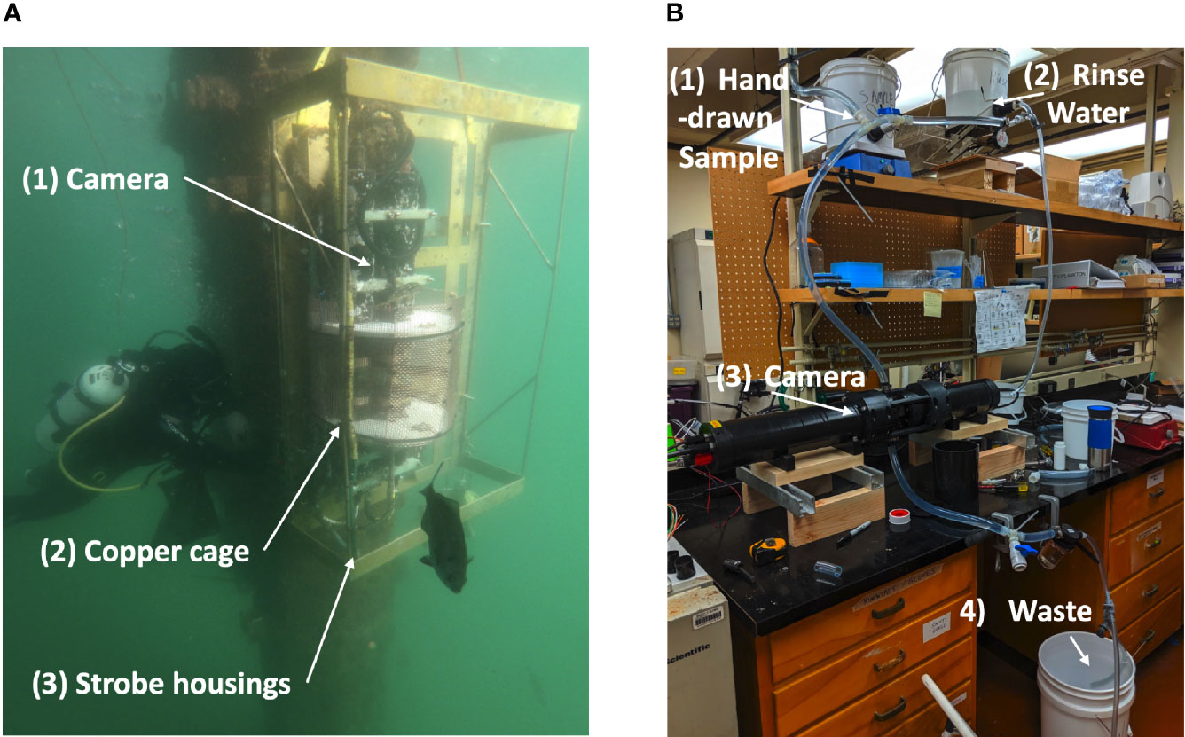
Figure 1 The Imaging Systems. (A) SPC-Pier, SPC-MICRO Underwater Camera. (B) SPC-Lab, Benched laboratory configuration of SPC-MICRO.

The SPC-Lab is a reconfigured benchtop version of the SPC-Pier. To support the imaging of hand drawn samples, it was augmented with a gravity flow water system so that each 8L water sample passed through a clear acrylic chamber positioned in the field of view of the system (Figure 1B). The sample was put through the system at a constant flow rate by routinely replenishing the elevated water bucket with more seawater to maintain a minimum of 2 L of fluid. The flow system was flushed with filtered seawater between samples to prevent cross-contamination.

2.3 Species Selection and Manual Classification

To form a data set for comparing the observed image counts from the two SPC systems with those of the Lab-micro, a team of 3 taxonomists sorted all images collected by both SPCs into 10 classification categories, or classes: 9 taxonomy-based categories that captured each of the target organisms (Figure 2) in the 30 µm and 60 µm size range, and a category ‘other’ that included images of remaining organisms and particles imaged by the system. The ‘other’ class is necessary to give both the taxonomists and the automated classifiers a place to put ambiguous objects and avoid high false-positive rates (Dhamija et al., 2018).

FIGURE 2

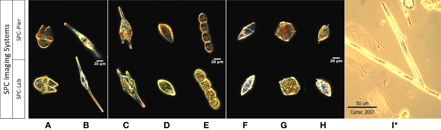
Figure 2 Images of 9 taxa from the SPC-Pier, SPC-Lab systems. (A–I) Akashiwo sanguinea, Ceratium furca, Chattonella spp., Cochlodinium spp., Gyrodinium spp., Lingulodinium polyedra, Prorocentrum micans, and Pseudo-nitzschia spp. (I)* Is a lab microscopy photo of Pseudo-nitzschia sp. as the SPC imaging systems produced unsuitable images.

2.4 Sample Selection

Over the course of 5 months, 43 independent plankton samples were acquired via Lab-micro, SPC-Lab, and SPC-Pier. After a preliminary data analysis, a subset of 26 days were deemed suitable for analysis as there were complementary Lab-micro samples with suitable abundances. We note that these abundances were suitable if, at least, tens of organisms were sampled on a fraction of the days. Using the data from the 26 days, a data set consisting of the measurement of plankton “counts” using 5 methods (Figure 3) was assembled: (i) traditional microscopy counts provided by SCCOOS (Lab-micro), (ii) manual classification of (SPC-Lab), (iii) automated classification, using a CNN, of images collected by the SPC-lab system (SPC+CNN-Lab), and, similarly for images collected by the in situ SPC system, (iv) manual (SPC-Pier) and (v) automated (SPC+CNN-Pier) classification of images collected by the SPC-Pier.

FIGURE 3

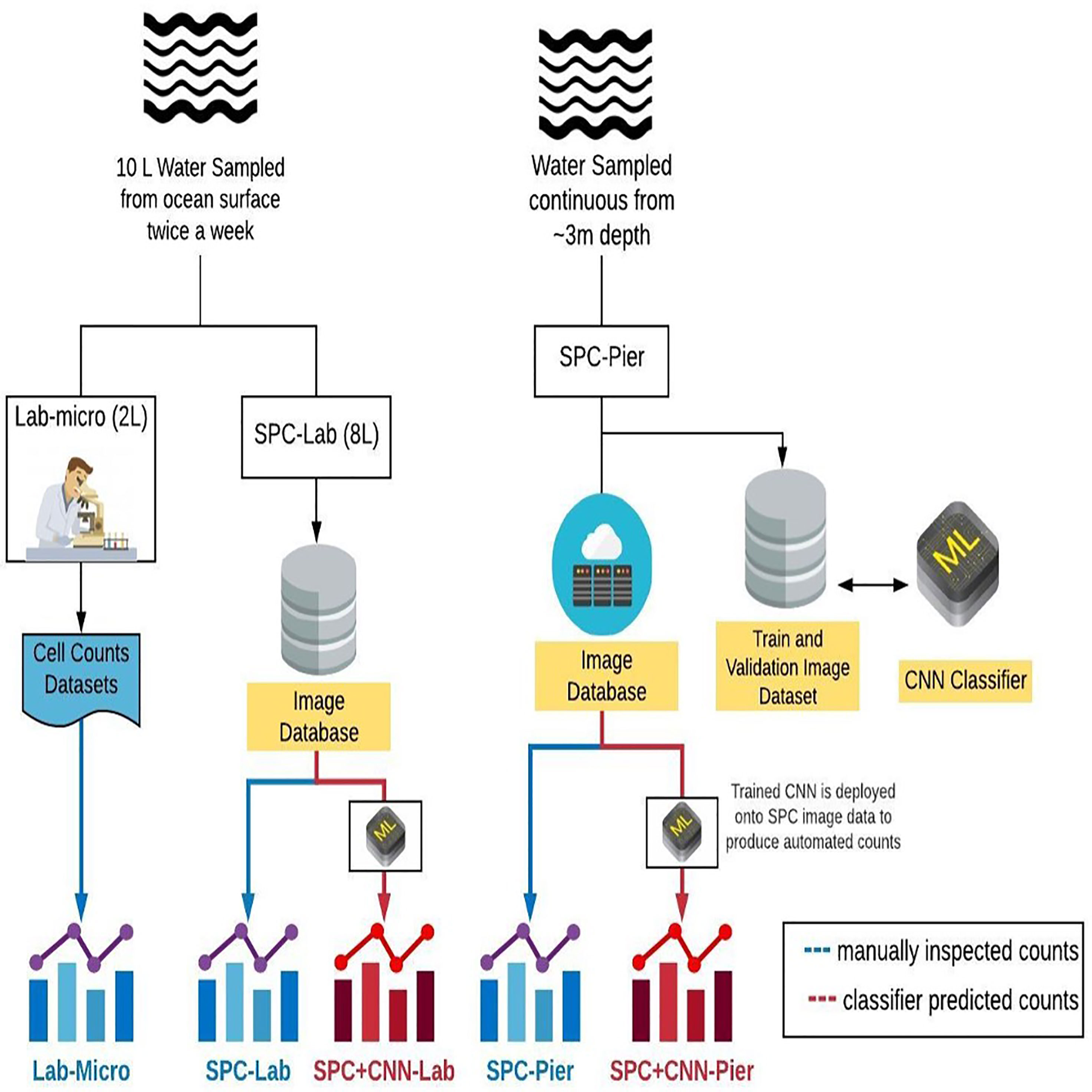
Figure 3 A diagram that compares the sampling methods and the 5 resultant data sets: Lab-micro, SPC-Lab, SPC+CNN-Lab, SPC-Pier and SPC+CNN-Pier.

2.5 Automated Imaging Classification Using Convolutional Neural Networks

To test the accuracy of automated image classification, we trained a collection of convolutional neural networks (SPC+CNN-Lab and SPC+CNN-Pier) and tested them on SPC-Lab and SPC-Pier images. The details of the implementation of the convolutional neural network methods are described below.

In training the Neural Networks we use the Residual Neural Network (He et al., 2015) architecture with 18 layers (ResNet-18). The relatively shallow network design is quick to train and less likely to overfit to the relatively small training sets we collected (Tetko et al., 1995). Network training followed standard practices in the machine learning literature, namely using stages of training, cross-validation, and testing (Table 1).

TABLE 1

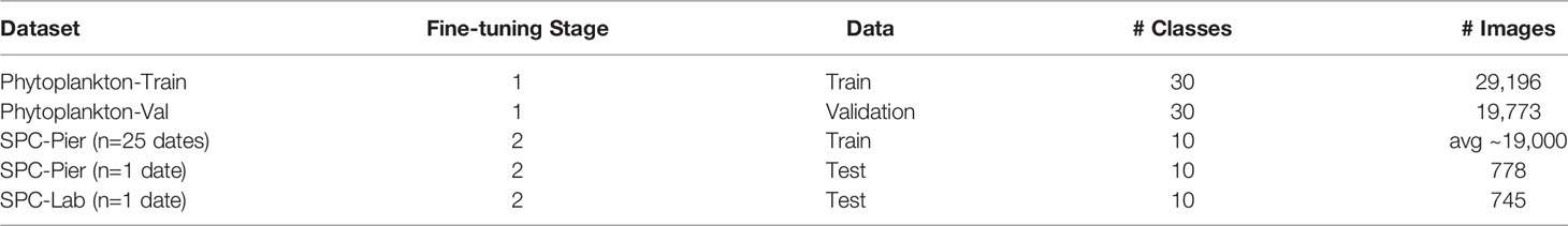
Table 1 Overview of training, validation, and test datasets to train the SPC+CNN.

In all experiments, images were subject to random affine transformations – rotations and translations. This type of data augmentation enables the creation of additional training examples. Prior to the random affine transformations, images are padded into a square image and resized into 224 x 224 pixels. All networks were trained with the cross-entropy loss for 50 epochs. However, throughout each phase of the training procedure, the loss was weighted inversely proportionally to the class distribution of the corresponding training dataset, to mitigate potential class imbalance problems (Wang et al., 2017). Note this also includes recomputing the weight of the loss of each during cross-validation. Model weights that achieved the lowest loss on the validation set during training the 50 epochs were utilized.

The SPC+CNN for both lab and pier was trained in two fine tuning stages: (i) We fine-tuned a ResNet-18 pre-trained on the ImageNet database (Deng et al., 2009) with SPC phytoplankton images. (ii) The resulting network was again fine-tuned on just the ten classes of interest using images collected by either SPC-Pier or SPC-Lab. Fine tuning repurposes the parameters of a network trained for a particular task to a different target. The procedure reduces training time and improves accuracy when training with small datasets (Yosinski et al., 2014). Double fine tuning further adapts each network to subtle differences between the SPC-Pier and SPC-Lab data after learning more general representations of plankton (Orenstein and Beijbom, 2017).

The first fine-tuning step uses a labeled phytoplankton training set from the SPC-Pier system that comprised of 37,147 images spanning 51 classes (Kenitz et al., 2022). This dataset was produced by 15 expert taxonomists and 5 non-taxonomists from the US West Coast during a two-day workshop whose main goal was to collect images for training the CNNs. This workshop dataset came from an earlier portion of the SPC-Pier time series and has no temporal overlap with the images acquired in our experiment. Experts sorted the annotated images into 44 taxonomic classes and 7 noise categories, which included the 9 species of interest. The workshop dataset was adjusted by combining categories of the same species tagged with semantic descriptors such as the number of cells (e.g., Ceratium furca pair vs. single) and eliminating categories with fewer than 300 images. This resulted in a total of 30 classes, 24 identifiable species and 6 noise categories. 80% of the 36,496 images were then randomly chosen for training (Phytoplankton-Train) and the remaining 20% used for validation (Phytoplankton-Val) (Table 1).

The second fine-tuning step had two objectives: (i) force the network to recognize only the 9 species of interest and the background class ‘other’ of our study; and (ii) account for dataset shift, the well-known property of classifiers to be sensitive to changes in the input data, both the appearance of the images and the relative distribution of the classes between training and testing (Moreno-Torres et al., 2012; He et al., 2015; González et al., 2019; Orenstein et al., 2020b). In this step, the classifier is fine-tuned to the collected SPC-Pier dataset, which was partitioned in a leave one-out cross-validation manner for training and testing. Specifically, the model is trained on data from all dates from the SPC-Pier except for one, which is used as a held-out test set (Table 1). The same procedure is repeated several times with each sampled date being used as a held-out set once, and performance metrics are averaged across all 26 days. The training sets for each cross-validation iteration contain approximately 39,000 images, and test sets respectively holding out 745 and 778 for the SPC-Pier and SPC-Lab.

In implementing the first stage, the base ResNet-18 model pretrained on ImageNet was fine-tuned for 50 epochs on the 30-class phytoplankton taxonomy workshop dataset. Model weights that achieved the lowest loss on the validation set during the 50 epochs were utilized. In this stage, the model achieved an accuracy of 95.5% on the Phytoplankton-Train set and accuracy of 95.2% on the Phytoplankton-Val set. The second stage was initialized with the model weights learned in the first stage, where the final layer was replaced with a layer of 10 outputs (9 categories of interest plus Other). Fine-tuning to the leave-one-out cross-validation training datasets was performed for an additional 50 epochs with model weight selection corresponding to the lowest training loss. This resulted in a collection of 26 trained models, where each model is tested on an independent date from the SPC-Pier and SPC-Lab dataset.

All models were trained with an initial learning rate of 0.001 and a batch size of 16 using the Adam optimizer (Kingma and Ba, 2014). Models were trained on an NVIDIA Titan Xp GPU. Python code used to train and evaluate the models is available at https://github.com/hab-spc/hab-ml.

There are several examples of dataset shift between our training sets, notably the slight variations in illumination between images captured by the SPC-Pier and SPC-Lab systems (Figure 2). The restriction of fine-tuning to only the SPC-Pier image dataset is specifically designed to examine the potential effects of dataset shift when the classifier is deployed on a new target domain, in our case the SPC-Lab. Training on SPC-Pier and testing on SPC-Lab data is a proxy for the more general transfer of a classifier trained on an in-situ imaging system to an in vitro imaging system.

2.6 Analyses of the Three Sampling Methods

To compare the three sampling methods, we used the total number (counts) of organism identification for each of the 10 categories collected on each of the 26 independent days. Given the species-specific counts, we performed 1) an assessment of the classifier performance and 2) a comparison between the Lab-micro counts and SPC+CNN counts. A comparison between the Lab-micro counts and manually enumerated SPC counts is also included to establish a baseline unaffected by CNN classifier errors. Although relative abundance is a widely used measure of plankton distributions, we use the number of counts of each species as a function of date, for two reasons: (1) Comparisons of relative abundance are sensitive to numerical instability caused by frequent counts of 0 or 1. (2) The effective interrogation volume of the SPC systems varies from species to species, due to both the focus dependent darkfield imaging as well as the effects of random orientations. As such, an important aspect of our work is the estimation of an “effective sampling volume” for each species as elaborated below.

2.6.1 Volume Computation Analyses

In all experiments, the volume V_Lab-micro of water used by lab procedure was standardized to 1.76 mL, while the counts of the SPC-Pier system were integrated over 2000 seconds of images taken at 8 Hz, resulting in 16,000 images. Under the assumption that the concentration of species counted by each method is the same,

$\begin{array}{ll}\frac{{\text{C}}_{\text{SPC}+\text{CNN}}}{{\text{V}}_{\text{SPC+CNN}}}=\frac{{\text{C}}_{\text{Lab}-\text{micro}}}{{\text{V}}_{\text{Lab}-\text{Micro}}},& \text{Equation 1}\end{array}$

where V_SPC-CNN is the effective volume imaged by the SPC system and C denotes counts. Now, defining the ratio α between the two volumes as

$\begin{array}{ll}{\text{V}}_{\text{SPC}+\text{CNN}}=\alpha {\text{V}}_{\text{Lab}-\text{micro}}& \text{Equation 2}\end{array}$

leads to the linear relationship

$\begin{array}{ll}{\text{C}}_{\text{SPC}+\text{CNN}}=\alpha {\text{C}}_{\text{Lab}-\text{micro}},& \text{Equation 3}\end{array}$

between SPC+CNN and Lab-micro raw counts. This was the model used to relate the SPC+CNN counts of both the Pier and lab implementations to Lab-micro counts in our study. The scaling factor α was estimated by computing a linear regression between each pair of counting methods.

2.6.2 Counting Analyses

Counts are compared across the 3 sampling methods, for both manually enumerated SPC and automated SPC+CNN counts. A separate model is fit for each of the 9 species using the linear regression model of (3) across all 3 pairs: SPC+CNN-Lab vs. Lab-micro; SPC+CNN-Pier vs. Lab-micro; and SPC+CNN-Pier vs. SPC+CNN-Lab. The model of (3) was fit with a linear-linear least squares estimator, assuming zero intercept. However, for display purposes, the data was transformed to a log scale. Given the computed linear regression between each pair of counting methods, quantitative comparisons are obtained by computing the Pearson correlation coefficient, a measure of linear correlation between two variables, and the percentage R²of the variance explained by the model relative to the total variance. In conjunction with the factor α, these measurements express how related the counting methods are.

2.6.3 Classification Analyses

Our collection of double fine-tuned classifiers is applied to the 26 daily test sets from which 21,211 images were extracted from the SPC-Lab and 20,148 images from the SPC-Pier that were then manually classified into the 10 categories. CNN Performance results are then averaged across the test sets. Classification performance is assessed by 1) accuracy (ACC), the fraction of correct predictions, 2) mean class accuracy (MCA), the average correct predictions over each individual class, and 3) the F1 score, a commonly used metric for scoring class-imbalanced problems. Together, these metrics capture both model generalization ability and bias towards highly populated classes – ACC characterizes the overall classifier performance while MCA and F1 scores assess how well the system does on a per-class basis. Significant differences between the three metrics indicate that a method favors common classes while underperforming for rare ones.

3 Results

Given the 26 independent samples, the datasets were largely dominated by the ‘other’ category (83% of the SPC-Pier total and 92% of the SPC-Lab total). The resulting manual counts are denoted as SPC counts. CNN-produced counts on the same dataset are denoted SPC+CNN counts. Lab-micro counts were produced by a biologist, using traditional microscopy.

3.1 Analysis of the Neural Net Results

In general, Lab-micro collected more total counts of the 9 target species, over the set of images, than the SPC systems (Figure 4A). Averaged over all 26 independent samples, Lab-micro count data was predominantly composed of 3 common species: Pseudo-nitzschia spp., Lingulodinium polyedra, and Prorocentrum micans (Figure 4B). The latter two also dominated SPC-Lab and SPC-Pier counts. However, in the case of the SPCs, the Pseudo-nitzschia spp. counts were notably fewer. Although there is some uncertainty in the inability of the SPCs to reliably detect the Pseudo-nitzschia spp., we suspect that it is likely because the thickness of this pennate diatom is close to the resolution limit of the system as well as the fact that a needle like structure, when subject to a uniformly random 2-dimensional view will be difficult to see in many of its orientations. The remaining taxa of interest, namely Akashiwo sanguinea, Ceratium falcatiforme or C. fusus, Ceratium furca, Chattonella spp., Cochlodinium spp., and Gyrodinium spp., were more often observed by the SPCs than the Lab-micro suggesting that the methodology has some taxonomic dependence.

FIGURE 4

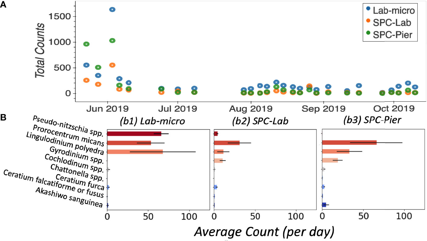
Figure 4 Enumerated plankton taxa. (A) Time series of total counts as obtained by traditional methods (LAB-micro) and manual image classification of lab samples (SPC-Lab) and in situ (SPC-Pier). (B) Average count per day per species collected by each method.

Inspection of the confusion matrices for the CNN performance of SPC-Pier versus SPC-Lab (Figure 5A) confirmed that the CNN performed significantly better on the SPC-Pier than on the SPC-Lab data, as expected from the MCA and F1 score difference shown in Table 2. For half of the tested species (Akashiwo sanguinea, Ceratium furca, Cochlodinium spp., Lingulodinium polyedra, Prorocentrum micans) the accuracy dropped more than 10% from SPC -Pier to SPC-Lab, especially Lingulodinium polyedra (Figure 5B). This is a manifestation of the domain shift between the SPC-Pier and SPC-Lab imaging methods: the lab flow-through system appeared to result in more out-of-focus images that rendered the species differentiation more difficult. This was not unexpected, given that the model is only trained on SPC-Pier data, however, it does illustrate that deployment of the same imaging system can vary, likely due to difference in lighting and any orientation effects that are due to flow.

FIGURE 5

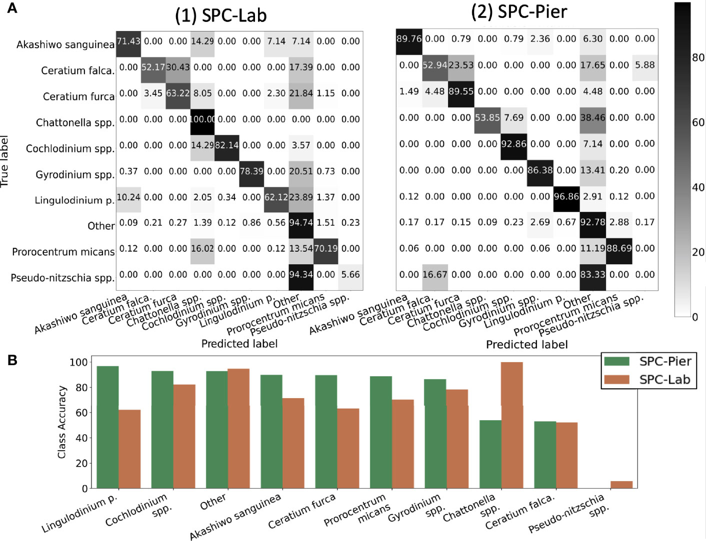
Figure 5 Quantification of the classification accuracy for SPC test sets. (A) Confusion Matrix. (B) Diagonal class accuracies of confusion matrix sorted in a descending fashion from left to right.

TABLE 2

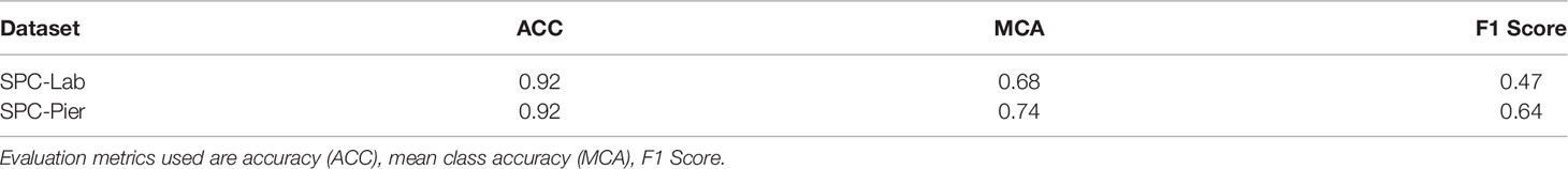
Table 2 Average classification results of a double fined-tuned model tested on independent held out samples collected by the SPC-Pier and SPC-Lab.

3.2 Classification Performance and Comparison of the Lab Micro vs SPC+CNN

Results indicate that the CNN achieved averaged test accuracies of 92% on both the SPC-Lab and SPC-Pier data (Table 2). The averaged ACC, MCA, and F1 Score performance was measured for a CNN tested on independent samples from the 26 SPC-Pier and SPC-Lab image datasets. The MCAs were lower (68 and 74%) suggesting an unbalanced performance across classes. This discrepancy between the metrics is originated by class population imbalance, due to the fact that some species were observed relatively rarely under the SPC setting (e.g. Ceratium falcatiforme or C. fusus, Chattonella spp., and Pseudo-nitzschia spp.). This results in less training data to effectively learn the species’ morphology. The F1 scores were the lowest of the three (.47 and.64), due to the CNNs’ frequent overestimation of the count of HAB species, which is penalized in the F1 score for poor precision. These results show that the CNN performs with high accuracy for the classes that are relatively abundant in the training data. Class imbalance in the training dataset can have a large effect on the learned model and is a well-established feature of training CNNs on natural populations.

The Pearson correlation analysis on the intermediary comparison of the Lab-micro and manually enumerated SPC counts (Figure 6) reveals high-to-very high correlations between the sampling methods on 4 out of the 9 species – Akashiwo sanguinea, Cochlodinium spp., Lingulodinium polyedra, and Prorocentrum micans – representing a mix of abundant and rare organisms (Figure 6A). The comparison for Ceratium furca revealed moderate correlations between both SPC methods and the Lab-micro (0.58 and 0.70). The other 4 species, Ceratium falcatiforme or C. fusus, Chattonella spp., Gyrodinium spp., and Pseudo-nitzschia spp., demonstrated a pattern of low correlation scores scoring correlation scores for two out of the three pairs.

FIGURE 6

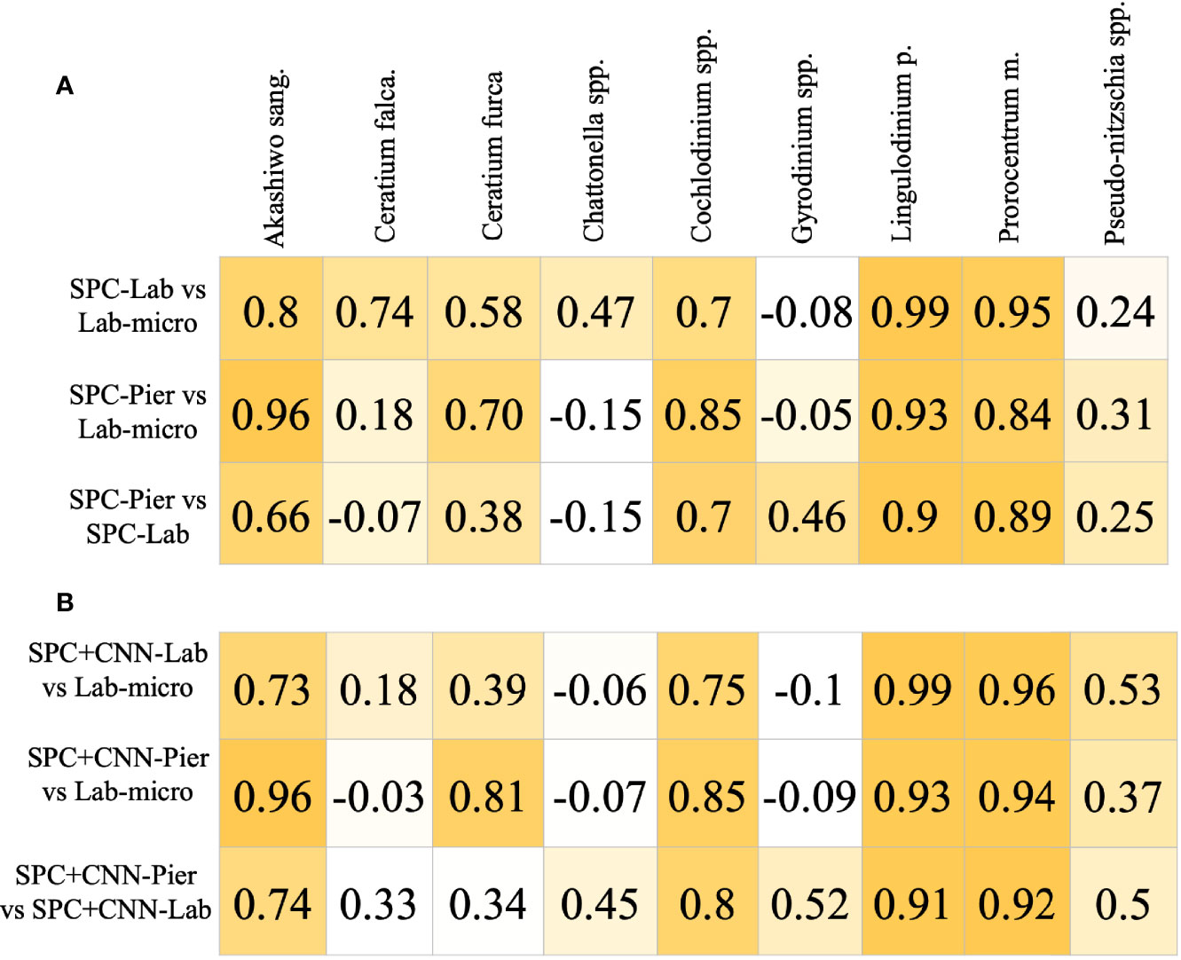
Figure 6 Pearson Corrélation Coefficient Matrices. Each row compares two of the resultant data and/or CNN estimation of taxonomic presence. Each column is a corresponding species. Coefficient values are color coded with respect to the species correlation value of the compared setting, in an ascending fashion. (A) Correlation of Lab-micro vs. manually enumerated SPC counts. (B) Correlation of Lab-micro vs. SPC+CNN counts.

In general, the SPC+CNN vs. Lab-micro correlations produced similar results to the baseline correlation values between the manually enumerated SPC vs. Lab-micro counts (Figure 6B). The same 4 species that previously produced high-to-very high correlations were consistent when using SPC+CNN counts, with correlation value differences up to 10%. The correlation differences were due to the previously mentioned unbalanced performances across the classes from the SPC+CNN, that arises from using imbalanced training data. In the case of the SPC+CNN-Lab vs. Lab-micro, we observed that many correlation scores dropped, which can be attributed to the domain-shift problem.

Figures 7, 8 display the linear fit between the enumerated counts for each of the sampling methods across the various taxa as computed by the regression model across the 3 possible data sources (Lab-micro, SPC+CNN-Lab and SPC+CNN-Pier). As can be seen, the proportionality approximation conveys that the SPC+CNN-Pier’s sampling of an aggregate volume over the 2000 seconds recorded nearly twice the number of images of the SPC+CNN-Lab. In addition, a majority of the five species showed non-existing-to-poor linear relationships between the Lab-micro and SPC+CNN counts. The linear fit for the Pseudo-nitzschia spp. showed little ability to model the relationship between the SPC+CNN and Lab-micro, as the SPCs detected the species poorly. Gyrodinium spp. were mostly absent from the Lab-micro, preventing a comparison via linear regression between the sampling methods. Species that had previously demonstrated low classification performance resulted in poorer relationships when computing the linear regression for the CNN-based pairs of counting methods. Compared to the manually enumerated-based linear regressions, Ceratium falcatiforme or C. fusus, and Chattonella spp. showed small R² values and fit to the slopes across all 3 possible pairs, suggesting that, possibly, poor classification performance negatively impacted the linearly modeled relationships. Ceratium furca also showed some fluctuations when comparing automated vs manual regressions, but generally showed only a lack of a linear relationship between the two data generation methods (Figure 7). Figure 8 shows the other 4 species where, we note, Akashiwo sanguinea and Cochlodinium spp. demonstrated a poor fit to the linear correlation while the L. polyedra and the P. micans were quite good with R² scores of (0.97, 0.89). We note that these two species had the highest number of counts across all three sampling methods and, conjecturally, the highest concentrations.

FIGURE 7

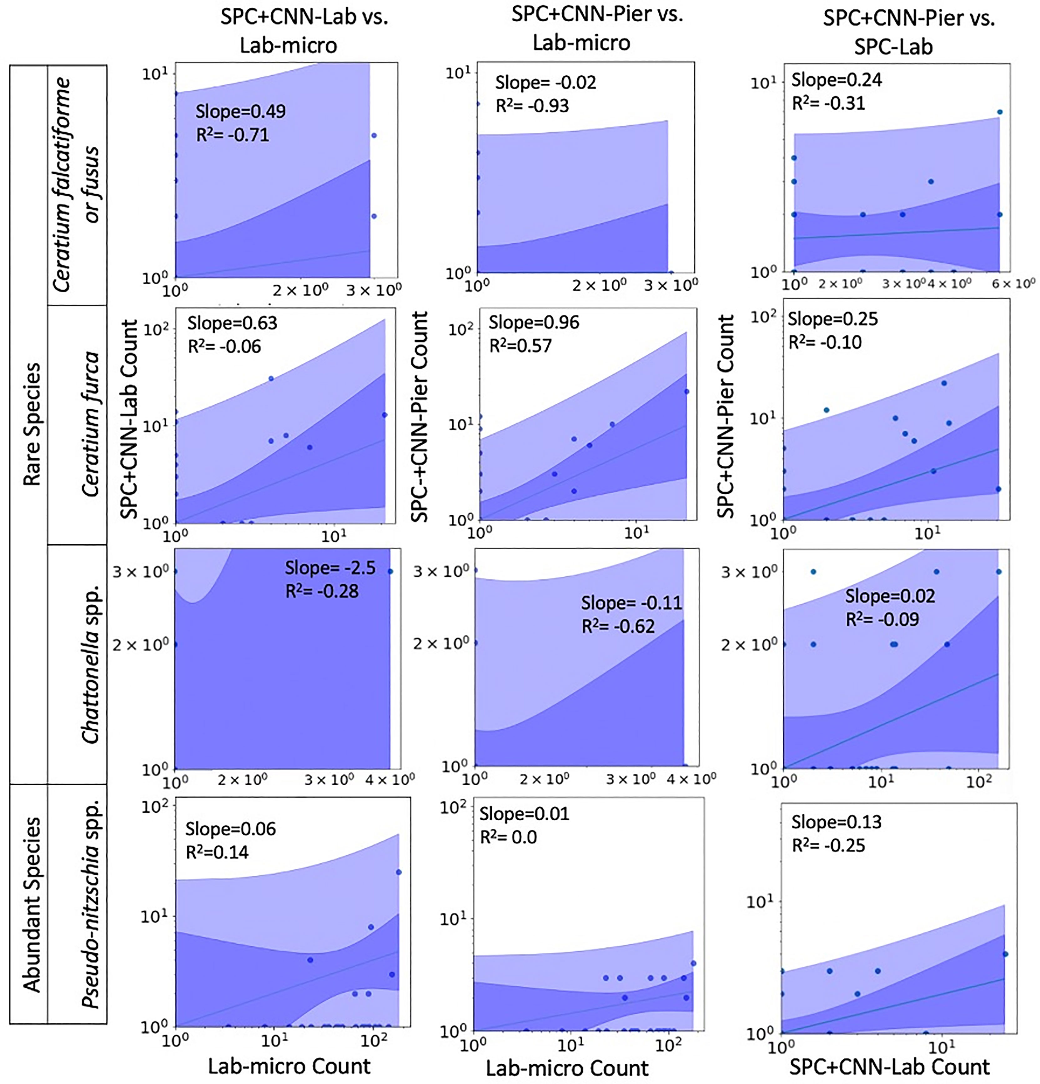
Figure 7 Relationships between counts of Lab-micro and SPC+CNN methods (less abundant species). Columns highlight pairs of counting methods, rows demarcate species. The solid line indicates a linear regression model that is coupled with multiple shaded areas indicating the 95% prediction (dark shade) and confidence interval (light shade). The slope and R² of the model fit are indicated.

FIGURE 8

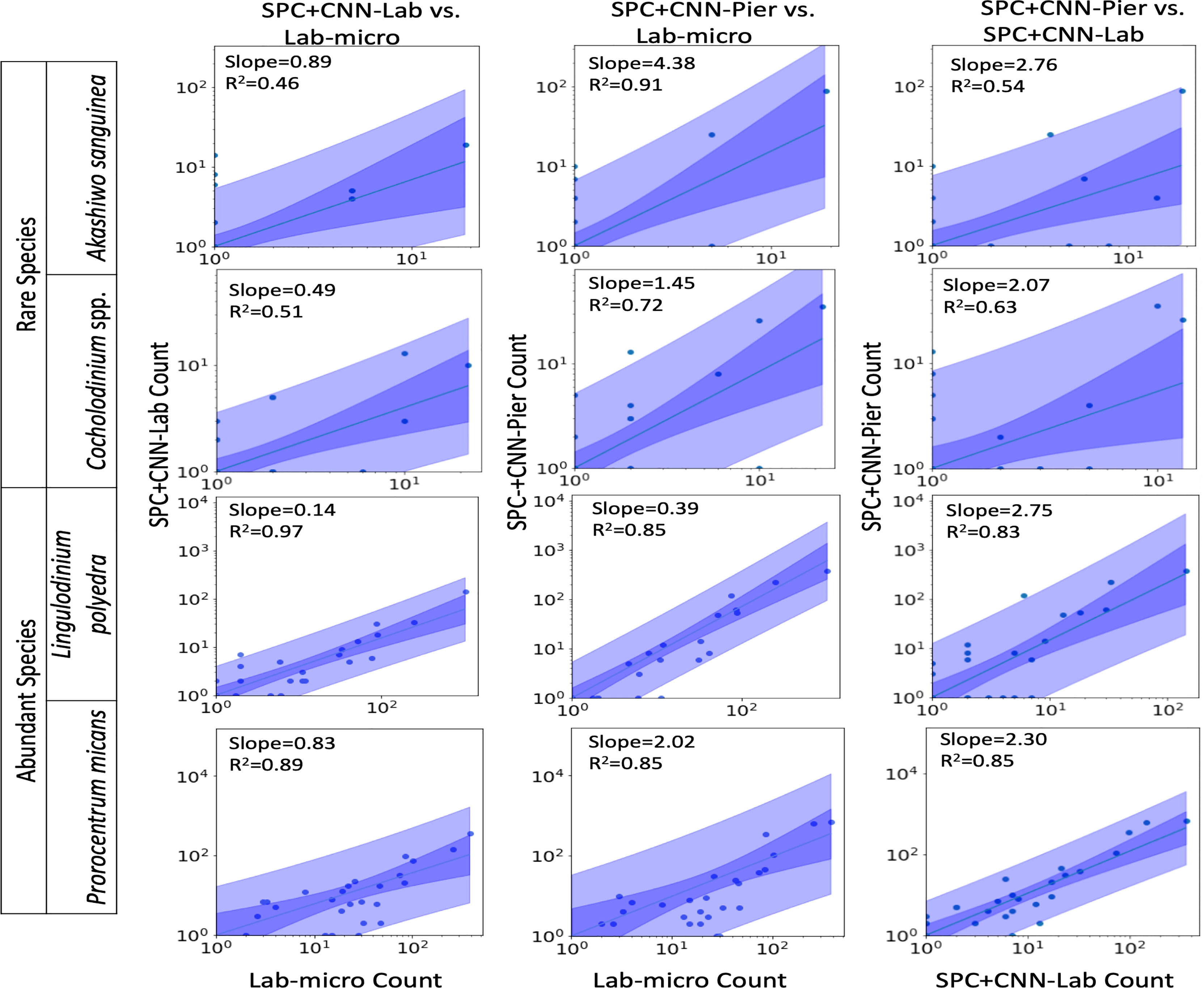
Figure 8 Relationships between counts of Lab-micro and SPC+CNN methods. Columns highlight pairs of counting methods, rows demarcate species. The solid line indicates a linear regression model that is coupled with multiple shaded areas indicating the 95% prediction (dark shade) and confidence interval (light shade). The slope and R² of the model fit are indicated. Note that data is displayed logarithmically but was fit linearly.

As shown in Figure 8, in a manner like the results of the Pearson correlation analysis for the pair of SPC+CNN-Pier vs. Lab-micro, we found high R² values for two of the less-abundant species (Akashiwo sanguinea, Cochlodinium spp.), and two of the more-abundant species (Lingulodinium polyedra, Prorocentrum micans). We also observed that the sizes of the prediction and confidence bands were related to the frequency of occurrence of the species. The two abundant species showed much narrower prediction and confidence bands, in contrast to the two rare species, which exhibited wider bands. Discrepancy of the size of the bands could be due to the low cell counts of the relatively rare species.

3.3 Volume Computation

An important feature of this work is the computation of the “effective sampling volume” for the SPC+CNN results. This then permits the estimate of abundance. Considering the most abundant and highly correlated species (Lingulodinium polyedra and Prorocentrum micans) equation (3) can be used to compute this volume using the slope of the fit as shown in Figure 7. Given that this slope is (0.39, 2.02) for (L. polyedra, P. micans) and that the reported Lab-micro samples a 1.76 mL volume, our cumulative sampling volume for 2000 seconds of images at 8 Hz is (0.69, 3.56) mL. Then, the “effective sampling volume” per image is estimated as (0.043, 0.22) μL after dividing by the 16000 frames. We note that the R² values for the other 4 categories were too low to be considered and are therefore not reported.

3.3 Continuous Observation Data

One major advantage of in situ microscopes like the SPC-Pier system is that they can observe plankton continuously in time. This permits post processing with a variable integration time to compute species dependent total counts. In this study, we used a 2000 second integration window that provided 16,000 image samples (at 8 Hz) that occurred over the period from the end of May until October 2019 (Figure 9). Here, the continuous grey line indicates counts of the 4 species that were most confidently estimated from the SPC+CNN-Pier during both the lab sampling occurrences as well as other times where there were no manually collected samples. We note that there was an increase in the Akashiwo sanguinea and Cochlodinium spp. during and in-between the lab samples as well as the absence of increased abundance for the Lingulodinium poleydra as well as the Prorocentrum micans that were not observed by the Lab-micro sampling as it was less frequent. The results highlight the advantages of continuous sampling that is facilitated by an in situ instrument. Moreover, the agreement when both the Lab-micro and the SPC+CNN-Pier data were available provides support to interpret the SPC+CNN-Pier system as valid, with, naturally, some error bound.

FIGURE 9

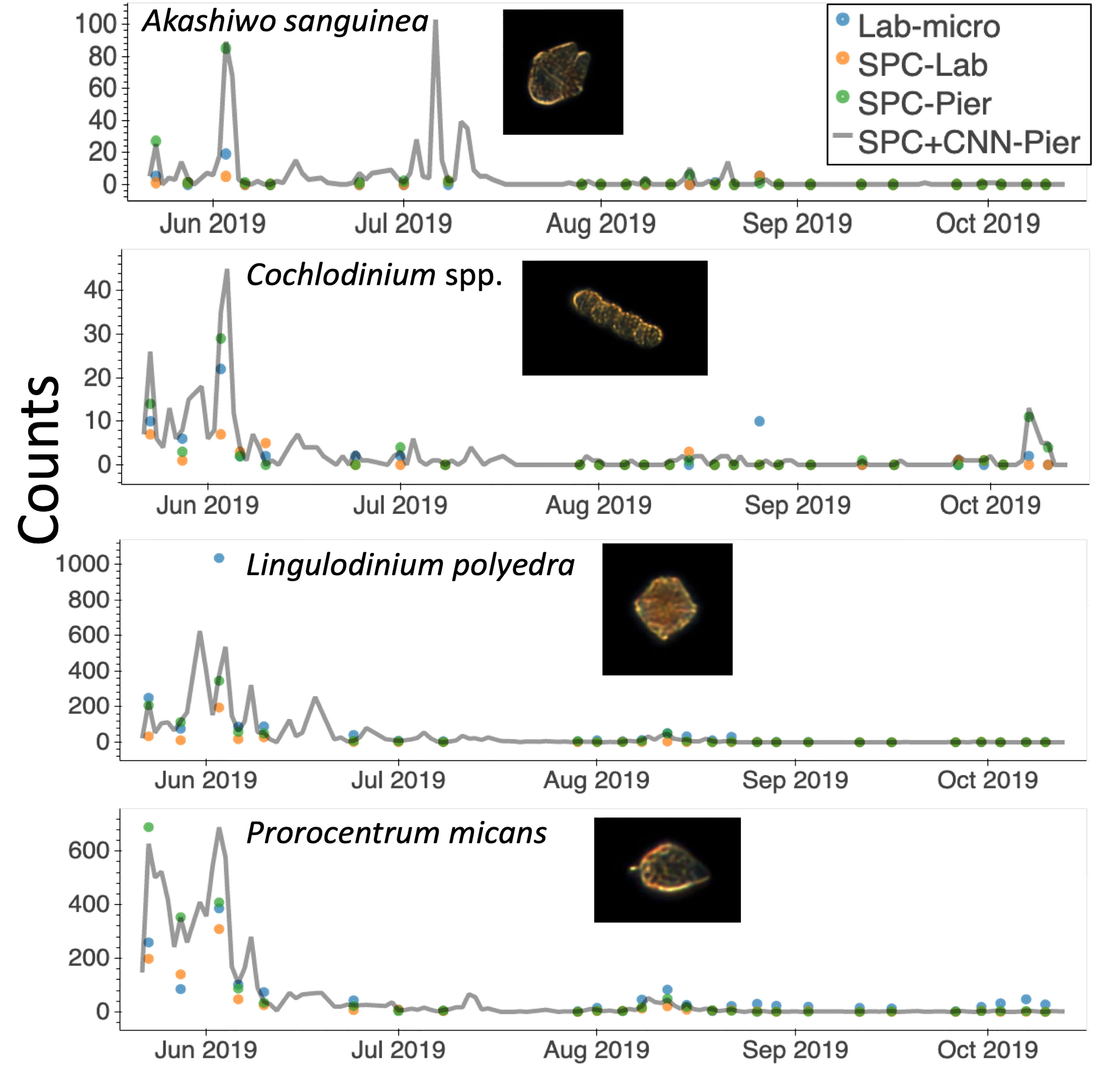
Figure 9 A time series of species presence via “counts” or number of observations by the SPC-pier and the SCCOOS monitoring program during 2019. Automated image classification was used to produce counts on continuous periods. Most of which were not sampled by the SCCOOS program. Plots are shown for only the highly correlated abundant and rare species.

4 Discussion

In recounting the goals of the work reported here, we first sought to explore the ability of CNNs to correctly classify the images that were recorded from the SPC systems. Although lab-based identification of the phytoplankton species is well established, the correspondence between the traditional methods and our dark-field microscopes had not been established. In examining the potential differences between the two methods, Lab-micro vs. SPC+CNN, there are several factors to consider: the samples observed by the SPC microscopes experience range-dependent defocus that is a necessary consequence of the dark-field illumination. In addition, since the SPC microscopes image organisms that are freely drifting in the field of view of the system, a natural assumption is that their orientation, relative to the viewpoint of the camera, is uniformly distributed. In contrast to larger zooplankton, such as copepods, our organisms of interest have fewer morphological differences that are also confounded by the aspect-dependent views acquired. This makes the identification more difficult for automated systems as well as taxonomists viewing the resultant SPC images.

In considering the success of the CNNs to classify the species present in the images, we found that the imbalanced nature of datasets significantly influenced the performance of the system. Class imbalance is a well-studied problem that exists in many real-world ocean ecosystem datasets (e.g. WHOI-plankton: (Orenstein et al., 2015), EILAT and RAMAS coral dataset (Shihavuddin, 2017) in which rare species have far fewer images than abundant species). To combat this problem, we applied transfer learning from a less-imbalanced and filtered dataset to a more-imbalanced and unfiltered one. We also applied cost-sensitive learning, one of the techniques commonly used to improve the performance of class imbalanced classification (Wang et al., 2017). However, the comparatively low performance on rare classes suggests a limited capability of our techniques to mitigate the class imbalance problem. For model improvement, it would be worth experimenting with other methods, such as an ensemble of CNN models (Lumini and Nanni, 2019) or applying transfer learning by pre-training with class-normalized data (Lee et al., 2016). Class imbalance can also be addressed by collecting data over an extended period, especially days with significant presence of the organisms from the classes under-populated in our training set. This is left for future studies.

Compared to the class imbalance problem of the SPC+CNN, domain shift is less discussed in deep learning applications in the ecological literature. However, our results suggest that this problem deserves critical consideration when deep learning systems are to be deployed in an environment different from that used for training. Many zooplankton detection systems, such as ZooplanktoNet (Dai et al., 2016) and Zooglider (Whitmore et al., 2019), did not explicitly address and investigate their deep learning models’ capability to transfer across domains. When trained purely on SPC-Pier image data, our model was not able to replicate its high performance to the SPC-Lab data, showing noticeably lower-class accuracies (for example for Prorocentrum micans or Lingulodinium polyedra) relative to the SPC-Pier. In future research, experimenting with other domain adaptation techniques, such as similarity learning (Pinheiro, 2018), or image-to-image translation (Murez et al., 2018), can help further improve our model. Solving the domain shift problem is essential to ensuring the reliability of deep learning automated systems in different environments.

Considering the nine species, or classification categories, investigated here, the significant correlation between the Lab-micro counts and the SPC+CNN-Pier data for Prorocentrum micans and Lingulodinium polyedra indicates that, under the environmental and lab identification procedures developed here, the in situ system counts can be transformed into estimates of concentration that are consistent with traditional microscopy observations. These correlations were also consistent when using the manually enumerated SPC counts instead of the SPC+CNN. The use of the multiplicative scaling factor α in our volume computation analysis mitigates these effects.

Both the SPC+CNN methods and Lab-micro show gaps in their ability to detect certain species. Firstly, Lab-micro only detected Gyrodinium spp. on one day, while both SPC methods detected it on more than 20 of the 26 days. This is, presumably, due to the formaldehyde treatment that leads to dissolution and subsequent misidentification of “naked” species like Gyrodinium spp. (Costas et al., 1995). On the other hand, the SPC methods have problems detecting Pseudo-nitzschia spp. Whether this is due to the inefficiency of the darkfield imaging technique or, rather, effects related to their chain-like structure when viewed in 3D is unknown. We do note, however, that there may be some advantages to observing settled samples.

The other major goal of this research was to estimate the “effective sampling volumes” so that abundance could be estimated from the SPC+CNN-Pier data. Here, we note that, as reported on the web site, (spc.ucsd.edu) the SPC2 camera used here has a “high-resolution image volume” of 0.1 μL and a “Blob detection volume” of 10 μL. The sample volumes reported in Table 3 of 0.043 μL and 0.22 μL for Lingulodinium polyedra and Prorocentrum micans, respectively, for the SPC+CNN-Pier are not inconsistent, likely due to the system’s single view angle resulting in ambiguities that prevent the unique identification of the species. We also note that in comparing the SPC+CNN-Lab values vs Lab-micro, the proportionalities indicate that the lab system detected approximately half of those detected by the SPC+CNN-Pier. The discrepancy may be because the SPC-Lab samples were taken from the near-surface of the ocean (~ 0.5 m), whereas the SPC-Pier samples from a tidally dependent depth of 3 m. The differences may also arise from orientation-dependent effects that result from the water flowing past the SPC-Lab, or differences in the two optical systems, such as illumination intensity. Less-abundant species (e.g., Akashiwo sanguinea and Cochlodinium spp.) had reasonable fits between the SPC-Pier and the Lab-micro, with the SPC-Pier having a larger slope and hence, a larger estimated sampling volume. However, the uncertainty of these values is higher due to the small number of samples.

TABLE 3

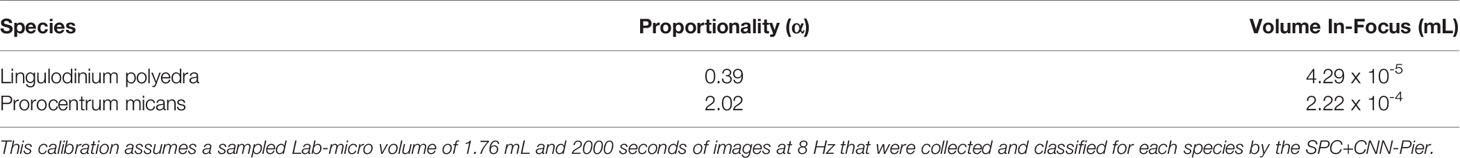
Table 3 Calibrated SPC+CNN-Pier Sampling Volume Per Image.

A distinguishing feature of this analysis is that the “effective sampling volumes” as computed via comparison with the Lab-micro calibrations are different for each species (e.g., Lingulodinium polyedra and Prorocentrum micans). These differences in estimated sampling volumes were not entirely unanticipated, as our dark-field illumination setup acquires an orientation-dependent image of these organisms, causing CNNs and expert taxonomists to be less capable of determining the exact identity of each species. Consequently, our linear fit for each of the species has a different slope, leading to different effective sampling volumes that are species dependent.

An important aspect of in situ sampling is that it is capable of detecting organisms on a 24/7 basis: the in situ microscope can provide continuous, real-time sampling during periods when there was no manual data collection (Figure 9). The period from May to October 2019 provided roughly 128k images via the automated sampling. The values obtained for Lingulodinium polyedra and Prorocentrum micans study showed realistic abundance increases and decreases of both, that occurred before and after a detected bloom. Rarer taxa, such as Akashiwo sanguinea and Cochlodinium spp., showed similar trends, but increases in abundance recorded by the imaging system were missed by the manual sample collection. Although a more detailed analysis would be needed to estimate the confidence in these observations, it seems that these transient changes in abundance were simply undetected because of the less frequent sampling by the Lab-micro. This, in turn, highlights the need for real-time continuous monitoring with less human effort. Furthermore, the low counts generated by the SPC systems between July and October indicated that there were no significant blooms during that time. Given the continuous nature of the SPC data stream, a set of algorithms could be implemented to deploy adaptive sampling that would improve the dynamic range of lab quantification.

One advantage of systems like SPC+CNN that produce real-time data is their potential for use as an early detection system. Data-driven insights would then inform decision making in monitoring programs, such as SCCOOS, for which shore station leaders have limited information on the daily abundance level of the HAB species. For example, previous studies show that it can be advantageous to know the initial and final periods of a bloom (Stroming et al., 2020). Stroming et al. (2020) showed the socioeconomic benefit of early HAB detection and estimated a saving of $370,000 following the early warning of a 2017 cyanoHAB event in Utah Lake. Given the statistically robust signals found in the present study for estimating HAB abundances, the recommended next steps would be to explore the use of the SPC for supporting decision-making in such settings.

5 Comments and Recommendations

The SPC+CNN workflow has shown its capability to provide real-time, high accuracy detection of certain HABs species, such as Akashiwo sanguinea Cochlodinium spp., Lingulodiniumpolyedra and Prorocentrum micans. Although its performance is species-dependent, it has shown a high correlation with the Lab-micro counts in certain cases. Moreover, this automated workflow can detect rare species more frequently than the manual method. It also minimizes manual labor and can provide continuous sampling at a high spatial and temporal resolution. All of these benefits make the SPC+CNN a potentially important tool with the capability to advance the study of imaging, recognition, and monitoring of HAB-related phytoplankton. The results suggest that image-based monitoring systems, supported by high-throughput automated classifiers, can be a reliable alternative to time-consuming manual sampling campaigns. Moreover, our experimental techniques and analyses provide a framework for future intercalibration studies of innovative new plankton sampling modalities.

Data Availability Statement

The raw data supporting the conclusions of this article will be made available by the authors, without undue reservation.

Author Contributions

KTL conceived the ideas and designed the methodology along with JSJ; ECO, MLC, KMK and SS collected the data; DR built the lab imaging instrument; ZY and PM trained the classifiers; KL, ZY, and AS analyzed the data; KL, JJ, NV, ECO, and PJSF led the writing of the manuscript. All authors contributed to the article and approved the submitted version.

Funding

The authors are grateful to the National Science Foundation for funding this research under Grant #1546351 and Grant # 1546305 that was awarded from the Div of Information and Intelligent Systems.

Conflict of Interest

The authors declare that the research was conducted in the absence of any commercial or financial relationships that could be construed as a potential conflict of interest.

Publisher’s Note

All claims expressed in this article are solely those of the authors and do not necessarily represent those of their affiliated organizations, or those of the publisher, the editors and the reviewers. Any product that may be evaluated in this article, or claim that may be made by its manufacturer, is not guaranteed or endorsed by the publisher.

References

Beers J. R., Stewart G. L. (1970). The Preservation of Acantharians in Fixed Plankton Samples1. Limnol Oceanog. 15 (5), 825–827. doi: 10.4319/lo.1970.15.5.0825

CrossRef Full Text | Google Scholar

Castellani C. (2010). Plankton: A Guide to Their Ecology and Monitoring for Water Quality. J. Plankt. Res. 32 (2), 261–262. doi: 10.1093/plankt/fbp102

CrossRef Full Text | Google Scholar

Costas E., Zardoya R., Bautista J., Garrido A., Rojo C., López-Rodas V. (1995). Morphospecies Vs. Genospecies in Toxic Marine Dinoflagellates: An Analysis of Gymnodznium Catenatum/Gyrodinium Impudicum and Alexandrium Minutum/a. Lusitanicum Using Antibodies, Lectins, and Gene Sequences1. J. Phycol. 31 (5), 801–807. doi: 10.1111/j.0022-3646.1995.00801.x

CrossRef Full Text | Google Scholar

Cowen R., Greer A., Guigand C., Hare J., Richardson D., Walsh H. (2013). Evaluation of the In Situ Ichthyoplankton Imaging System (Isiis): Comparison With the Traditional (Bongo Net) Sampler. Fish. Bull. 111, 1–12. doi: 10.7755/FB.111.1.1

CrossRef Full Text | Google Scholar

Culverhouse P. F., Macleod N., Williams R., Benfield M. C., Lopes R. M., Picheral M. (2014). An Empirical Assessment of the Consistency of Taxonomic Identifications. Mar. Biol. Res. 10 (1), 73–84. doi: 10.1080/17451000.2013.810762

CrossRef Full Text | Google Scholar

Dai J., Ruchen Wang H. Z., Guangrong J., Xiaoyan Q. (2016). “Zooplanktonet: Deep Convolutional Network for Zooplankton Classification.” in Oceans 2016 (Shanghai: IEEE), 1–6.

Google Scholar

Deng J., Dong W., Socher R., Li L. J., Li K., Fei-Fei L. (2009). “Imagenet: A Large-Scale Hierarchical Image Database,” in 2009 IEEE Conference on Computer Vision and Pattern Recognition. 248–255.

Google Scholar

Dhamija A. R., Günther M., Boult T. E. (2018). Reducing Network Agnostophobia. Adv. Neutr. Inform. Proc. Syst. 31, 1811.04110. doi: 10.48550/arXiv.1811.04110

CrossRef Full Text | Google Scholar

Ellen J. S., Graff C. A., Ohman M. D. (2019). Improving Plankton Image Classification Using Context Metadata. Limnol. Oceanog.: Methods 17 (8), 439–461. doi: 10.1002/lom3.10324

CrossRef Full Text | Google Scholar

Field C. B., Behrenfeld M. J., Randerson J. T., Falkowski P. (1998). Primary Production of the Biosphere: Integrating Terrestrial and Oceanic Components. Science 281 (5374), 237. doi: 10.1126/science.281.5374.237

PubMed Abstract | CrossRef Full Text | Google Scholar

González P., Castaño A., Peacock E. E., Díez J., Del Coz J. J., Sosik H. M. (2019). Automatic Plankton Quantification Using Deep Features. J. Plankt. Res. 41 (4), 449–463. doi: 10.1093/plankt/fbz023

CrossRef Full Text | Google Scholar

Hamner W. M., Madin L. P., Alldredge A. L., Gilmer R. W., Hamner P. P. (1975). Underwater Observations of Gelatinous Zooplankton: Sampling Problems, Feeding Biology, and Behavior1. Limnol. Oceanog. 20 (6), 907–917. doi: 10.4319/lo.1975.20.6.0907

CrossRef Full Text | Google Scholar

He K., Zhang X., Ren S., Sun J. (2015). Deep Residual Learning for Image Recognition. ArXiv, 1512.03385. doi: 10.48550/arXiv.1512.03385

CrossRef Full Text | Google Scholar

Irisson J. O., Ayata S. D., Lindsay D. J., Karp-Boss L., Stemmann L. (2022). Machine Learning for the Study of Plankton and Marine Snow From Images. Annu. Rev. Mar. Sci. 3, 14. doi: 10.48550/arXiv.1512.03385

CrossRef Full Text | Google Scholar

Iyer N. (2012). Machine Vision Assisted In Situ Ichthyoplankton Imaging System.

Google Scholar

Karlson B., Cusack C., Bresnan E. (2010). Microscopic and Molecular Methods for Quantitative Phytoplankton Analysis (UNESCO). Available at: https://repository.oceanbestpractices.org/handle/11329/303.

Google Scholar

Kenitz K. M., Orenstein E. C., Roberts P. L., Franks P. J., Jaffe J. S., Carter M. L., et al. (2020). Environmental Drivers of Population Variability in Colony-Forming Marine Diatoms. Limnol. Oceanog. 65 (10), 2515–2528. doi: 10.1002/lno.11468

CrossRef Full Text | Google Scholar

Kenitz K. M., Anderson C. R., Carter M. L., Eggleston E., Seech K., Shipe R., et al. (2022). Training Image Data For: Environmental and Ecological Drivers of Harmful Algal Blooms in the Southern California Bight. UC San Diego Library Digital Collections. doi: 10.6075/J00865GT

CrossRef Full Text | Google Scholar

Kim H.-J., Miller A. J., McGowan J., Carter M. L. (2009). Coastal Phytoplankton Blooms in the Southern California Bight. Prog. Oceanog. 82 (2), 137–147. doi: 10.48550/arXiv.1512.03385

CrossRef Full Text | Google Scholar

Kingma D. P., Ba J. (2014). Adam: A Method for Stochastic Optimization. ArXiv. Prepr. ArXiv., 1412.6980. doi: 10.48550/arXiv.1512.03385

CrossRef Full Text | Google Scholar

LeCun Y., Bengio Y., Hinton G. (2015). Deep Learning. Nature 521 (7553), 436–444. doi: 10.1038/nature14539

PubMed Abstract | CrossRef Full Text | Google Scholar

Lee H., Park M., Kim J. (2016). “Plankton Classification on Imbalanced Large Scale Database Via Convolutional Neural Networks With Transfer Learning,” in 2016 IEEE International Conference on Image Processing (ICIP). 3713–3717. doi: 10.1109/ICIP.2016.7533053

CrossRef Full Text | Google Scholar

Lefebvre K. A., Powell C. L., Busman M., Doucette G. J., Moeller P. D., Silver J. B., et al. (1999). Detection of Domoic Acid in Northern Anchovies and California Sea Lions Associated With an Unusual Mortality Event. Nat. Tox. 7 (3), 85–92. doi: 10.1002/(sici)1522-7189(199905/06)7:3<85::aid-nt39>3.0.co;2-q

CrossRef Full Text | Google Scholar

Lombard F., Boss E., Waite A. M., Vogt M., Uitz J., Stemmann L., et al. (2019). Globally Consistent Quantitative Observations of Planktonic Ecosystems. Front. Mar. Sci. 6. doi: 10.3389/fmars.2019.00196

CrossRef Full Text | Google Scholar

Lumini A., Nanni L. (2019). Deep Learning and Transfer Learning Features for Plankton Classification. Ecol. Inf. 51, 33–43. doi: 10.1016/j.ecoinf.2019.02.007

CrossRef Full Text | Google Scholar

Luo J. Y., Irisson J.-O., Graham B., Guigand C., Sarafraz A., Mader C., et al. (2018). Automated Plankton Image Analysis Using Convolutional Neural Networks. Limnol. Oceanog.: Methods 16 (12), 814–827. doi: 10.1002/lom3.10285

CrossRef Full Text | Google Scholar

Moreno-Torres J. G., Raeder T., Alaiz-Rodríguez R., Chawla N. V., Herrera F. (2012). A Unifying View on Dataset Shift in Classification. Pattern Recog. 45 (1), 521–530. doi: 10.1016/j.patcog.2011.06.019

CrossRef Full Text | Google Scholar

Murez Z., Kolouri S., Kriegman D., Ramamoorthi R., Kim K. (2018). “Image to Image Translation for Domain Adaptation,” in Proceedings of the IEEE Conference on Computer Vision and Pattern Recognition. 4500–4509.

Google Scholar

Olson R. J., Sosik H. M. (2007). A Submersible Imaging-in-Flow Instrument to Analyze Nano-and Microplankton: Imaging Flowcytobot: In Situ Imaging of Nano- and Microplankton. Limnol. Oceanog.: Methods 5 (6), 195–203. doi: 10.4319/lom.2007.5.195

CrossRef Full Text | Google Scholar

Omori M., Hamner W. M. (1982). Patchy Distribution of Zooplankton: Behavior, Population Assessment and Sampling Problems. Mar. Biol. 72 (2), 193–200. doi: 10.1007/BF00396920

CrossRef Full Text | Google Scholar

Orenstein E. C., Beijbom O. (2017). “Transfer Learning and Deep Feature Extraction for Planktonic Image Data Sets,” in 2017 IEEE Winter Conference on Applications of Computer Vision (WACV). 1082–1088. doi: 10.1109/WACV.2017.125

CrossRef Full Text | Google Scholar

Orenstein E. C., Beijbom O., Peacock E. E., Sosik H. M. (2015). Whoi-Plankton-a Large Scale Fine Grained Visual Recognition Benchmark Dataset for Plankton Classification. ArXiv. Prepr. ArXiv., 1510.00745.

Google Scholar

Orenstein E. C., Kenitz K. M., Roberts P. L. D., Franks P. J. S., Jaffe J. S., Barton A. D. (2020b). Semi- and Fully Supervised Quantification Techniques to Improve Population Estimates From Machine Classifiers. Limnol. Oceanog.: Methods 18 (12), 739–53. doi: 10.1002/lom3.10399

CrossRef Full Text | Google Scholar

Orenstein E. C., Ratelle D., Briseño-Avena C., Carter M. L., Franks P. J. S., Jaffe J. S., et al. (2020a). The Scripps Plankton Camera System: A Framework and Platform for in Situ Microscopy. Limnol. Oceanog.: Methods 18 (11), 681–695. doi: 10.1002/lom3.10394

CrossRef Full Text | Google Scholar

Picheral M., Catalano C., Brousseau D., Claustre H., Coppola L., Leymarie E., et al. (2021). The Underwater Vision Profiler 6: An Imaging Sensor of Particle Size Spectra and Plankton, for Autonomous and Cabled Platforms. Limnol. Oceanog.: Methods 20 (2), 115–29. doi: 10.1002/lom3.10475.

CrossRef Full Text | Google Scholar

Picheral M., Guidi L., Stemmann L., Karl D. M., Iddaoud G., Gorsky G. (2010). The Underwater Vision Profiler 5: An Advanced Instrument for High Spatial Resolution Studies of Particle Size Spectra and Zooplankton. Limnol. Oceanog.: Methods 8 (9), 462–473. doi: 10.4319/lom.2010.8.462

CrossRef Full Text | Google Scholar

Pinheiro P. O. (2018). “Unsupervised Domain Adaptation With Similarity Learning,” in Proceedings of the IEEE Conference on Computer Vision and Pattern Recognition. pp 8004–8013.

Google Scholar

Salman A., Jalal A., Shafait F., Mian A., Shortis M., Seager J., et al. (2016). Fish Species Classification in Unconstrained Underwater Environments Based on Deep Learning. Limnol. Oceanog.: Methods 14 (9), 570–585. doi: 10.1002/lom3.10113

CrossRef Full Text | Google Scholar

Scholin C. A., Gulland F., Doucette G. J., Benson S., Busman M., Chavez F. P., et al. (2000). Mortality of Sea Lions Along the Central California Coast Linked to a Toxic Diatom Bloom. Nature 403 (6765), 80–84. doi: 10.1038/47481

PubMed Abstract | CrossRef Full Text | Google Scholar

Shihavuddin A. (2017). Coral Reef Dataset, v2. Mendeley Data. Available at: https://data.mendeley.com/datasets/86y667257h/2

Google Scholar

Sinha E., Michalak A. M., Balaji V. (2017). Eutrophication Will Increase During the 21st Century as a Result of Precipitation Changes. Science 357 (6349), 405–408. doi: 10.1126/science.aan2409

PubMed Abstract | CrossRef Full Text | Google Scholar

Smith J., Connell P., Evans R. H., Gellene A. G., Howard M. D. A., Jones B. H., et al. (2018). A Decade and a Half of Pseudo-nitzschia Spp. And Domoic Acid Along the Coast of Southern California. Harmf. Algae. 79, 87–104. doi: 10.1016/j.hal.2018.07.007

CrossRef Full Text | Google Scholar

Sosik H. M., Olson R. J. (2007). Automated Taxonomic Classification of Phytoplankton Sampled With Imaging-in-Flow Cytometry. Limnol. Oceanog.: Methods 5 (6), 204–216. doi: 10.4319/lom.2007.5.204

CrossRef Full Text | Google Scholar

Stroming S., Robertson M., Mabee B., Kuwayama Y., Schaeffer B. (2020). Quantifying the Human Health Benefits of Using Satellite Information to Detect Cyanobacterial Harmful Algal Blooms and Manage Recreational Advisories in U.S. Lakes. GeoHealth 4 (9), e2020GH000254. doi: 10.1029/2020GH000254

PubMed Abstract | CrossRef Full Text | Google Scholar

Tetko I. V., Livingstone D. J., Luik A. I. (1995). Neural Network Studies. 1. Comparison of Overfitting and Overtraining. J. Chem. Inf. Model. 35 (5), 826–833. doi: 10.1021/ci00027a006

CrossRef Full Text | Google Scholar

Utermöhl H. (1931). Neue Wege in Der Quantitativen Erfassung Des Plankton. (Mit Besonderer Berücksichtigung Des Ultraplanktons). SIL. Proc. 5 (2), 567–596. doi: 10.1080/03680770.1931.11898492

CrossRef Full Text | Google Scholar

Utermöhl H. (1958). Methods of Collecting Plankton for Various Purposes are Discussed. SIL. Communicat. 1953-1996 9 (1), 1–38. doi: 10.1080/05384680.1958.11904091

CrossRef Full Text | Google Scholar

Wang Y.-X., Ramanan D., Hebert M. (2017). “Learning to Model the Tail,” in Advances in Neural Information Processing Systems, vol. 30 . Eds. Guyon I., Luxburg U. V., Bengio S., Wallach H., Fergus R., Vishwanathan S., Garnett R. (Curran Associates, Inc), 7029–7039. Available at: http://papers.nips.cc/paper/7278-learning-to-model-the-tail.pdf.

Google Scholar

Whitmore B. M., Nickels C. F., Ohman M. D. (2019). A Comparison Between Zooglider and Shipboard Net and Acoustic Mesozooplankton Sensing Systems. J. Plankt. Res. 41 (4), 521–533. doi: 10.1093/plankt/fbz033

CrossRef Full Text | Google Scholar

Yosinski J., Clune J., Bengio Y., Lipson H. (2014). How Transferable are Features in Deep Neural Networks? Adv. Neural Inf. Process. Syst. 27. 1–9

Google Scholar