Coupled Coccolith-Based Temperature and Productivity High-Resolution Reconstructions in the Eastern Equatorial Pacific During the Last Deglaciation and the Holocene

We present a new high-resolution reconstruction of annual sea-surface temperatures (SSTa) and net primary productivity (NPP) using novel coccolithophore-based models developed for the Eastern Equatorial Pacific (EEP). We combined published coccolithophore census counts from core-tops in the Eastern Pacific with 32 new samples from the Equatorial region, to derive a new statistical model to reconstruct SSTa. Results show that the addition of the new EEP samples improves existing coccolithophore-based SST-calibrations, and allow reconstructing SSTa in the EEP with higher confidence. We also merged the relative abundance of deep-photic species Florisphaera profunda in the same surface sediment samples with existing calibration datasets for tropical regions, to reconstruct annual NPP. Both temperature and productivity calibrations were successfully applied to fossil coccolith data from Ocean Drilling Project Site 1240, in the EEP. The coccolith-based SSTa estimates show a cooling during the Last Glacial Maximum (LGM) and the Younger Dryas, and warming at the start of the Holocene. This pattern differs in the timing and magnitude of the temperature changes from other available SST-reconstructions based on biogeochemical and faunal proxies. We discuss these discrepancies to be the result of different proxy sensitivities to insolation forcing, seasonal bias, and/or preservation artifacts. Reconstructed annual NPP shows a general decreasing trend from the late last glacial period to recent times, which we relate to the weakening of wind-driven equatorial upwelling towards the Holocene. We also calculated carbon export using our SSTa and NPP reconstructions, and compared to other geochemical-based reconstructions for the same location. Our coupled SSTa-NPP reconstruction provides key data to more fully assess the evolution of primary and export productivity as well as organic carbon burial in the EEP, with implications for its role in global biogeochemical cycles across glacial terminations.

GRAPHICAL ABSTRACT

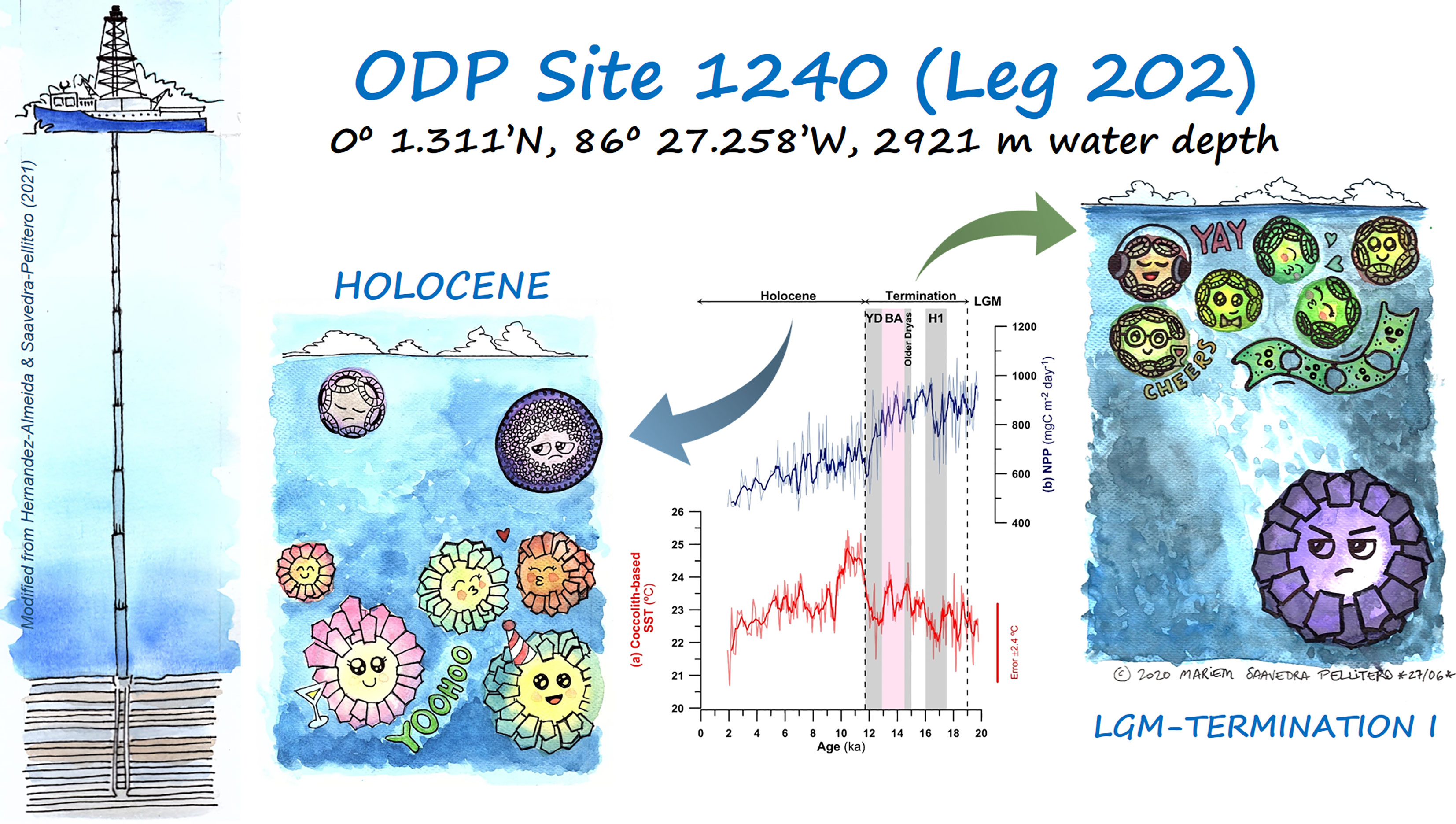
Graphical Abstract Estimated coccolith-derived sea surface temperature SSTa (°C, in red) and coccolith-derived Net Primary Productivity (NPP, mg C m^-2 day^-1, in blue) at ODP Site 1240, both with a 5-point running average smoothing. The vignettes depict two different scenarios, the first one during the Last Glacial Maximum/Termination I (with low % of Florisphaera profunda and high NPP) and the second one during the Holocene (with higher % of F. profunda and decreased NPP).

1 Introduction

The Eastern Equatorial Pacific (EEP) is an important region for Earth’s climate. Atmospheric-oceanographic perturbations (i.e. El Niño-Southern Oscillation, ENSO) and extended coastal and upwelling systems occurring in this region influence global climate and biogeochemical cycles in the ocean (e.g., Gu and Philander, 1995; Cane, 1998; Liu and Yang, 2003; Calvo et al., 2011; Costa et al., 2017; Lin and Qian, 2019). The EEP also accounts for 5–10% of the global oceanic net primary productivity (NPP) (Pennington et al., 2006). Mixed layer NPP is inversely correlated to sea surface temperature (SST) in this tropical region (Behrenfeld et al., 2006). When ocean stratification is relaxed, deep mixing brings cooler and nutrient-rich waters to the surface, fueling primary productivity (Behrenfeld et al., 2006; Schneider et al., 2008). The EEP shows large spatial gradients in chemical, physical and biological parameters, subject to strong seasonal and inter-annual variability (e.g., Strutton et al., 2008).

Holocene changes in the NPP and SST dynamics can be inferred from observations and model integrations (Behrenfeld et al., 2006; Timmermann et al., 2014; Krumhardt et al., 2016). These observations show that increasing influence of anthropogenic warming on marine ecosystems has led to a decrease of NPP in tropical regions (Behrenfeld et al., 2006), which is expected to get more pronounced in the coming decades (Laufkötter et al., 2015). Although contentious, recent studies have suggested that perturbations in the oceans could cause a tipping point in tropical SST and NPP in response to global warming, which would have impacts on the interconnected Earth biophysical systems, leading to long-term irreversible changes (e.g., Lenton et al., 2019). However, trends and feedbacks in the climate system are not easy to identify using the relatively short instrumental record, limited to just a few decades of observations (satellites), or a century at most (historical network of in-situ measurements). Palaeoclimatic information derived from sedimentary records provides additional constraints on the response of EEP regional SSTs and NPP to large global climate variations, such as the transition from the Last Glacial Maximum (LGM) to the Holocene (e.g., Leduc et al., 2010; Timmermann et al., 2014; Costa et al., 2017).

For the EEP there are a large number of SST reconstructions spanning the LGM to Recent, using a range of geochemical and biological SST proxies: Mg/Ca (e.g., Lea et al., 2006; Mix, 2006; Pena et al., 2008), alkenones (e.g., Koutavas and Sachs, 2008; Dubois et al., 2009; Schneider et al., 2010; Dubois et al., 2014), foraminifera-, diatom-, and radiolarian-based transfer functions (e.g., Pisias et al., 1997; Mix et al., 1999; Yu et al., 2012; Lopes et al., 2015), as well as $\text{TE}{\text{X}}_{86}^{\text{H}}$ (e.g., Shaari et al., 2013). These reconstructions are not all consistent (e.g., Kienast et al., 2013; Timmermann et al., 2014). For example, Mg/Ca-derived SSTs show cooling through the Holocene, whilst alkenone-derived SST show warming trends, although at different locations in the EEP (e.g., Leduc et al., 2010; Liu et al., 2014). These divergent responses are most likely due to proxy sensitivities to seasonal insolation changes (Leduc et al., 2010), or preservational artifacts and aliasing (Leduc et al., 2010; Dubois et al., 2014).

Reconstructions of LGM to Holocene EEP productivity also vary between proxies (e.g., Robinson et al., 2009; Schneider et al., 2010; Calvo et al., 2011; Kienast et al., 2013; Patarroyo and Martínez, 2015; Costa et al., 2017; Diz et al., 2018; Jacobel et al., 2020), with some proxy systems responding to multiple environmental factors (Jacobel et al., 2020; Studer et al., 2021). Sediment cores separated by just a few degrees of latitude, north and south from the Equator, show diverging trends in productivity-related proxies, most likely as a consequence of the strong gradients in nutrient regimes and variable oceanographic features (e.g., Dubois et al., 2010; Dubois and Kienast, 2011; Costa et al., 2017; Studer et al., 2021). Multi-proxy studies thus provide a fuller, and hopefully more accurate, reconstruction of the coupling between stratification and productivity through time, as well as the basis to consider the spatial variation in productivity regimes across the EEP.

Coccoliths, individual calcium carbonate platelets formed by coccolithophores (single-celled algae), are one of the major components of deep-ocean sediments and constitute a powerful micropaleontological tool to characterize environmental conditions of the past (e.g., Beaufort et al., 2001; Baumann and Freitag, 2004; Kameo et al., 2004; Agnini et al., 2017; Saavedra-Pellitero et al., 2019; Tangunan et al., 2020). Recent calibration studies have improved quantitative coccolithophore assemblage-based approaches for the reconstruction of multiple environmental variables (e.g., Saavedra-Pellitero et al., 2013; Ausín et al., 2015; Hernández-Almeida et al., 2019). A training set of coccolith assemblages in core-top sediments was developed to reconstruct SST in the south eastern Pacific (Saavedra-Pellitero et al., 2010; Saavedra-Pellitero et al., 2011; Saavedra-Pellitero et al., 2013), but has only been applied downcore at one high-latitude site in the Southeast Pacific (Ocean Drilling Project ODP Site 1233). The results of these coccolith-based SST reconstructions agreed well with other SST proxies at this site (Lamy et al., 2004; Kucera et al., 2005; Pisias et al., 2006; Abrantes et al., 2007; Lamy et al., 2007).

Satellite-derived NPP observations calibrated to the relative abundance of the tropical taxa Florisphaera profunda in surface sediments from the Indian Ocean and the South China Sea (Beaufort et al., 1997; Beaufort et al., 2001; Zhang et al., 2016) have been used to quantitatively reconstruct NPP in various regions (e.g., Tangunan et al., 2020). More recently, Hernández-Almeida et al. (2019) developed a global calibration comprising samples from all tropical regions, which considers the response of F. profunda to changes in NPP, and allows the reconstruction of NPP across all low-latitude regions with high confidence (e.g., Tangunan et al., 2021).

In this study, we extend these approaches by analyzing coccolith assemblages from a new set of surface sediment samples in the EEP, and merge this data with the dataset from Saavedra-Pellitero et al. (2010), to generate new coccolith-based calibrations to reconstruct both SST and NPP in the EEP region. We then apply both calibrations to the fossil coccolith assemblage at ODP Site 1240, located in the Panama Basin, to provide reliable high resolution NPP and SST quantitative reconstructions for the last 20 kyr covering the late last glacial period, Termination I, and the Holocene.

2 Study Area and Oceanographic Settings

The newly compiled dataset of sediment surface coccolithophore assemblages covers an area from 15.7°N to 50.7 °S and from 70.5°W to 110.6°W, ranging from the Equator to high-latitudes in the Southern Ocean (see Figure 1), including most of the Peru-Chile Current (PCC) system. The cold, low-salinity water of the PCC flows northward, and the southeast trade winds maintain the PCC and promote the Peruvian and the equatorial upwelling, which makes the EEP a highly productive area (Figure 1B) (Toggweiler et al., 1991). The PCC waters feed the South Equatorial Current, which flows west driven by the prevailing winds in the region. The North Equatorial Countercurrent represents the most important equatorial surface current flowing east (Tomczak and Godfrey, 1994), which is deflected to the north feeding the North Equatorial Current. The Equatorial Undercurrent flows eastward below the South Equatorial Current and provides nutrient-rich waters to the equatorial upwelling, controlling primary productivity in the region (Murray et al., 1994). The Equatorial Undercurrent continues eastward, feeding the Peruvian coastal upwelling (Toggweiler et al., 1991) and the Peru Undercurrent (Wyrtki, 1981; Strub et al., 1998).

FIGURE 1

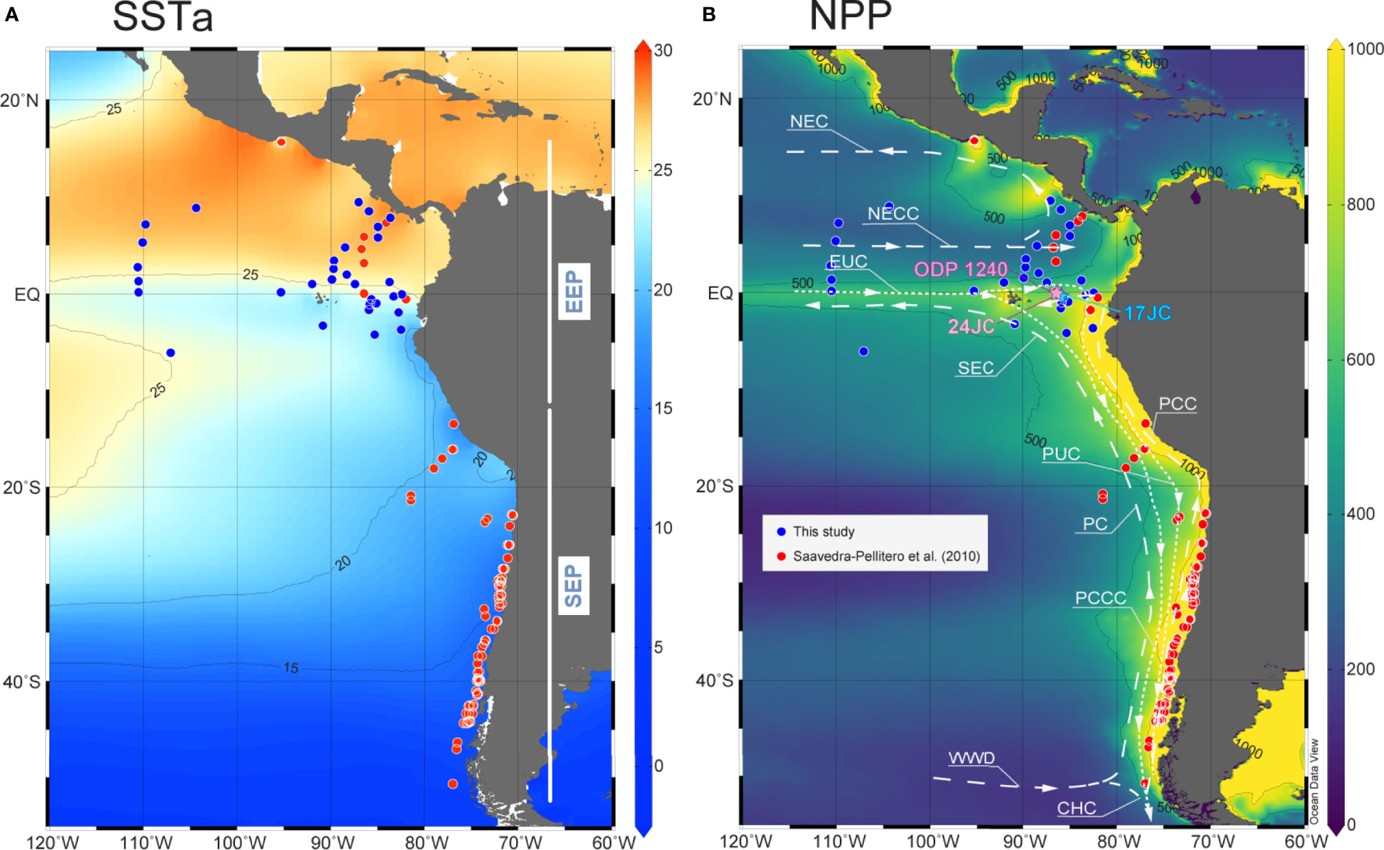
Figure 1 Study area. (A) Annual sea surface temperature (SSTa, in °C) from the World Ocean Atlas 2013 (WOA13) (Locarnini et al., 2013). (B) Annual mean of net primary productivity (NPP, in mg C m^-2 day^-1) estimated using the VGPM algorithm (Behrenfeld and Falkowski, 1997). The red (Saavedra-Pellitero et al., 2010) and blue (present study) dots indicate location of the surface sediment samples with coccolithophore assemblage data. ODP Site 1240, ME0005-24JC (24JC in the map), MV1014-02-17JC (17JC in the map) and the major surface and subsurface currents in the eastern Pacific Ocean (Strub et al., 1998; Feldberg and Mix, 2002; Fiedler and Talley, 2006) are shown: WWD, West Wind Drift; PC, Peru Current; PCC, Peru-Chile Current; PCCC, Peru-Chile Countercurrent; PUC, Peru Undercurrent; SEC, South Equatorial Current; EUC, Equatorial Undercurrent; NECC, North Equatorial Countercurrent and NEC, North Equatorial Current.

The geographic area that covers the whole surface sediment sample dataset is characterized by a strong gradient in annual mean temperatures, with SST ranging from ca. 28°C north of the Equator, to ca.~20°C in equatorial and Peru-Chile upwelling systems, down to 8°C in southern high latitudes (Figure 1A). In the EEP, the seasonal changes in SST are linked to shifts in the position of the Intertropical Convergence Zone (Wyrtki, 1966). Upwelling along the Equator and in the eastern boundary current, offshore Peru and Chile, supplies nutrient‐rich waters (Berger et al., 1987), resulting in high NPP values (up to 1000 mg C m^-2 day^-1) (Figure 1B). In contrast, productivity drastically decreases towards the Southern Pacific Gyre where nutrients are very limited. Productivity is lower during boreal winter at the Equator, although winds blowing from the Central American Cordillera cause localized upwelling and decrease of temperatures north of the Equator (Xie et al., 2005).

3 Material and Methods

3.1 Modern Coccolithophore and Environmental Data Sets

For the present study we considered new and published data (Table S1; Supplementary Material). The new dataset consists of 48 surface sediment samples retrieved between ca. 11°N and 12°S (core locations and sample codes can be found in Table S1). The uppermost centimetre was sampled from sediment cores retrieved between 152 and 5086 m water depth. Most of the samples are located above the present Carbonate Compensation Depth –CCD- (4000 m) and Carbonate Lysocline (3800 m) in the equatorial Pacific (Thompson, 1976; Farrell and Prell, 1989). Thirty two surface sediment samples were considered for this study (blue dots in Figures 1A, B), all above the CCD. A further 16 were found to be devoid of coccoliths and therefore excluded from the considered dataset. Based on published radiocarbon dating of planktonic forminifera shells from surface sediments of the EEP (e.g., Koutavas and Lynch-Stieglitz, 2003; Mekik, 2014; Studer et al., 2021) (Table S2; Supplementary Material) as well as on available literature focusing on the south-eastern Pacific (SEP) area (e.g., Abrantes et al., 2007; Saavedra-Pellitero et al., 2010; Saavedra-Pellitero et al., 2011; Saavedra-Pellitero et al., 2013) the age of the sediments can be regarded as no older than late Holocene to Recent, as it mostly lies between 0.79 and 3.57 Cal age ka BP.

The present study follows the coccolithophore taxonomy of Jordan and Kleijne (1994); Jordan et al. (2004), and the electronic guide to the biodiversity and taxonomy of coccolithophores Nannotax 3 (http://ina.tmsoc.org/Nannotax3/index.html) by Young et al. (2020), with few additional considerations, for instance small-sized Gephyrocapsa (< 3 µm) is referred here as small Gephyrocapsa, for consistency with Saavedra-Pellitero et al. (2010). Annual averaged present-day environmental variables such as the annual sea-surface temperature (SSTa) (Locarnini et al., 2013), annual-sea surface salinity (SSS) (Zweng et al., 2013), apparent oxygen utilization, as well as nitrate and phosphate contents obtained at 10 m water depth in the eastern Pacific Ocean (Garcia et al., 2014) were taken from the World Ocean Atlas 2013 (WOA 13), using Ocean Data View 5.3 (ODV) software (Schlitzer, 2021). NPP estimates were based on MODIS chlorophyll-a, SSTa and photosynthetic active radiation satellite data, using the standard vertically Generalized Production Model (VGPM) (Behrenfeld and Falkowski, 1997). These environmental data were interpolated to the geographic location of new surface sediment samples, and the ones from Saavedra-Pellitero (2010) to keep consistency in the data, using a weighted average gridding as implemented in ODV. Water depth and distance to the coast were also considered here. The first one refers to the depth at which the surface sediment sample was retrieved, in order to assess potential dissolution effects. The distance to the coast (in km) may control the amount of terrigenous material (including reworked material from continental shelves) delivered to the ocean.

3.2 Downcore Dataset: ODP Site 1240

ODP Site 1240 (Leg 202) is located in the southern Panama Basin (0° 1.311’N, 86° 27.258’W) at 2921 m water depth (Figure 1B). Studied sediments consist mostly of nannofossil ooze rich in foraminifera with varying amounts of diatoms, and rare siliciclastic components (Mix et al., 2003). The age model for the sedimentary sequence at ODP Site 1240 has previously been established by Pena et al. (2008), and it is based on radiocarbon ages of 11 samples of the planktonic foraminifera Neogloboquadrina dutertrei for the studied interval in the present work. ODP Site 1240 is ideally located to capture climate and oceanographic signals related to the past upwelling and biological production changes in the EEP, due to the relatively high sedimentation rates (allowing high temporal resolution studies), calcium carbonate content and general good preservation of carbonate microfossils (Mix et al., 2003). Additionally, the availability of multiple climate proxies at the ODP Site 1240 location (or nearby) is crucial in order to improve the reliability of climate reconstructions. The mean sedimentation rate varies from ~25 cm kyr^-1 during the Termination I to ~7 cm kyr^-1 during the late Holocene. For this study, a total of 270 samples were collected every centimetre covering the last 19.8 kyr (Table S3; Supplementary Material). The temporal average resolution of this study is 66 yr.

3.3 Sample Preparation and Microscope Observations

Slides were prepared following the well-established settling technique of Flores and Sierro (1997). Observations and coccolith counts were made with a Leica light microscope at 1000x magnification. A minimum of 500 coccoliths were counted per sample, ensuring that all species with an abundance above 1% were represented (Dennison and Hay, 1967; Fatela and Taborda, 2002). From the 270 samples considered for this study, 127 samples covering the Holocene were already available and therefore included (Cabarcos et al., 2014) (Table S1; Supplementary Material). The coccolith assemblage composition is reported in this work as relative abundance. Additionally, total absolute abundance of coccoliths (N, coccoliths per g of sediment) was calculated with the formula:

$\begin{array}{ll}N=\frac{n R^2 V}{r^{2 }g v}& \text{[Equation 1]}\end{array}$

where n is the number of coccoliths counted in a random visual field; R is the radius of the Petri dish used; V is the volume of buffered water added to the dry sediment; r is the radius of the microscope visual field; g is the dry sediment weight; and v is the volume of mixture pipetted. Knowing the dry density of the sediment and the sedimentation rate, it was possible to calculate the total coccolith accumulation rate (CAR) as follows:

$\begin{array}{ll}\mathrm{CAR}=Nds& \text{[Equation 2]}\end{array}$

where N is the absolute abundance of coccolithophores; d is the dry bulk density of the sediment (https://web.iodp.tamu.edu/), and s is the linear sedimentation rate.

3.4 Coccolith Preservation

A dissolution index was calculated to assess the potential effect of preferential carbonate dissolution on the coccolith assemblage. The CEX’ index (Boeckel and Baumann, 2004) represents the ratio between small and delicate E. huxleyi + small Gephyrocapsa (= small placoliths) and the strongly calcified Calcidiscus leptoporus as follows:

$\begin{array}{ll}\mathrm{CEX\prime }=\frac{\%\mathrm{ small placoliths}}{\%\mathrm{ small} \mathrm{placoliths} +\%\mathit{ C}\mathit{. leptoporus}}& \text{[Equation 3]}\end{array}$

CEX’ ranges from 0 to 1, with values closer to 1 suggesting a better preservation of coccoliths.

3.5 Statistical Analyses

A principal component analysis (PCA) was performed to explore the main gradients in the environmental dataset. The purpose of this analysis was to summarize the multivariate environmental data using components that explain the variance in the dataset (Davis, 1986; Harper, 1999). The ‘broken stick’ model was used to assess the significance of the PCA axes (Jackson, 1993).

Detrended correspondence analysis (DCA) with detrending by segments (Hill and Gauch, 1980) on the species data was used to estimate the length of the ecological gradient, to decide whether lineal or unimodal multivariate statistical methods should be used (Birks et al., 1990). As the length of the first DCA was shorter than 2 Standard Deviation (SD), i.e. 1.25 SD, we assumed that the species response was lineal, as it was in Saavedra-Pellitero et al., (2013), and applied the appropriate linear ordination method (Ter Braak, 1987; Ter Braak and Prentice, 1988). Redundancy Analysis (RDA) was performed on square root species abundances, with down-weight of rare species and scaling focused on inter-species distances, to explore the environmental-species relationships. We calculated the ratio of the first constrained eigenvalue to the first unconstrained eigenvalue (i.e. RDA1/PCA1 = λ1/λ2) to assess the significance of each environmental variable on the modern coccolith dataset (Juggins, 2013), with values >1 indicating a strong response of the assemblage to the variable of interest.

For the development of the transfer function, we used the well-stablished regression method Imbrie and Kipp factor analysis (IKFA) (Imbrie and Kipp, 1971), because it is suitable for short gradients. The coefficient of determination (R²) and root mean square of prediction (RMSEP) were assessed by bootstrapping cross-validation (999 permutation cycles) (Vaughan and Ormerod, 2005). The optimal number of factors in the final IKFA model was chosen by establishing a ≥5% improvement in RMSEP over alternatives with less components (Birks, 1998). Outliers were identified as those samples with absolute residuals (difference between observed and predicted values) higher than 2SD of the environmental variable of interest. Similarity between the modern and the fossil dataset was evaluated calculating the chord distance between both (or analogue distance) (Overpeck et al., 1985) (Figure S1A; Supplementary Material). To evaluate whether the variable in the final model was also significant for the downcore assemblage and ODP Site 1240, we used the statistical test developed by Telford and Birks (2011). This method compares the variance in the fossil assemblage explained by the environmental variable of interest with the proportion of the variance explained by randomly generated environmental variables (Figure S1B; Supplementary Material). The multivariate ordination analyses, transfer function model, significance and analogue test were performed with the R software (version 3.5; R Core Team, 2018), using the packages ‘rioja’ (Juggins, 2017), ‘vegan’ (Oksanen et al., 2019), ggpaleo (Telford, 2020), ‘palaeoSig’ (Telford, 2019) and ‘analogue’ (Simpson and Oksanen, 2020). Species thermal niche was calculated adapting the code used in Jonkers and Kucera (2019) (https://github.com/lukasjonkers/species_selection).

3.6 Past Primary Productivity Estimates

The percentage abundance of the deep-dwelling species Florisphaera profunda is a well-established proxy for primary productivity (Molfino and McIntyre, 1990b; Molfino and McIntyre, 1990a; Beaufort et al., 1997). The abundance of this species has been calibrated to satellite-derived NPP across multiple oceanic regions, at mid-to-low latitudes (Hernández-Almeida et al., 2019) resulting in the relationship:

$\begin{array}{ll}\mathrm{lo}{g}_{10} \left(\mathrm{Npp}\right) =3.11-0.01\left(\%\mathit{ F}.\mathit{ profunda}\right)& \text{ [Equation 4]}\end{array}$

In this calibration core-top dataset the EEP was only represented by 10 samples, taken from Saavedra-Pellitero et al. (2010). Here we re-evaluate and update the F. profunda-NPP relationship in the EEP with the addition of 32 new calibration points. This new calibration is then used to reconstruct NPP for the last 20 kry at ODP Site 1240.

3.7 Export Production Estimates

We calculated the export production (e_f) at ODP Site 1240 using the following equation from Laws et al. (2011) and our SSTa and NPP estimates:

$\begin{array}{ll}{e}_f= 0.04756 \left(0.78-\frac{0.43 \mathrm{SSTa}}{30}\right) \mathrm{NPP}{}^{0.307}& \text{[Equation 5]}\end{array}$

Additionally, the transfer efficiency (T_eff) was calculated for the neighbouring core ME0005-24JC using the equation from Henson et al. (2012):

$\begin{array}{ll}{T}_{\mathrm{eff}} = 0.196\left(\pm 0.006\right) – 0.066\left(\pm 0.004\right) \mathit{opal} + 0.017\left(\pm 0.004\right) \mathit{CaC}{\mathit{O}}_{\mathit{3}}& \text{ [Equation 6]}\end{array}$

Where opal is the Th-normalized opal flux and CaCO₃ is the Th-normalized carbonate flux (Kienast et al., 2007).

4 Results

4.1 Distribution of Coccoliths in Surface Sediment Samples From the EEP

Here we focus on core top assemblage data for the EEP sector, comprising the new dataset and a few surface sediment samples located between 15.7°N and 12°S published by Saavedra-Pellitero et al. (2010). There is a wide range of coccolith preservation state recorded across the study area (ranging from poor to good) but for most samples it is good, with a CEX’ generally >0.9 (Figure 2). The best-preserved coccoliths are recovered from sediments in the Panama Basin, whilst the most poorly preserved ones (or samples devoid of coccoliths) are found between ~6°N and ~12°N, ~7°S and ~13°S in the EEP region.

FIGURE 2

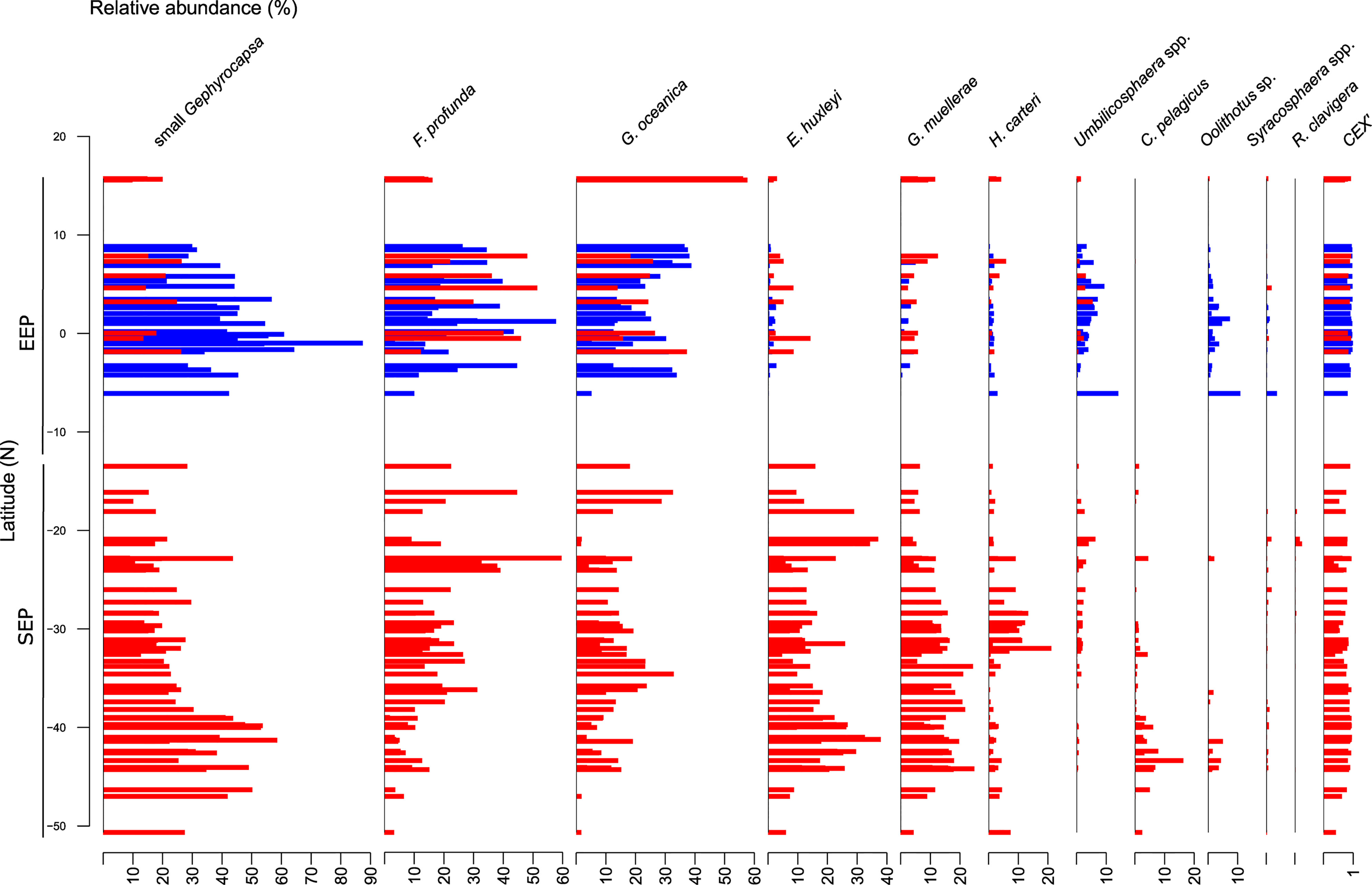
Figure 2 Relative abundance of the most important coccolithophore species (>1% on average) in the surface sediment samples (sorted by latitude) and CEX’ index. The red and blue bars correspond to the samples from Saavedra-Pellitero et al. (2010) and this study, respectively.

Gephyrocapsids are the most abundant coccolithophore taxa in the surface sediment samples from the EEP, with small Gephyrocapsa dominating assemblages (35.7% on average) and reaching highest relative abundances > 80% in the southern area of the Panama Basin, at ~1°S (Figure 2). The abundance of small Gephyrocapsa decreases from the Panama Basin towards northern latitudes. Gephyrocapsa oceanica is represented with a mean relative abundance of 23.9%, reaching a maximum of 57.7% offshore Mexico at ~15.6°S (Figure 2).

The lower photic zone taxa F. profunda is relatively common in the EEP region, with percentages ranging from 3.6% to 59.7%, and a mean of 26% (Figure 2). Gephyrocapsa muellerae occurs with a mean relative abundance of 2.6% and maximum of 12.5%, with low relative abundances in the EEP, which are similar to those of E. huxleyi with a mean abundance of 2.1% and a maximum of 14.2% at ~0.5°S (Figure 2). The abundance of Calcidiscus leptoporus varies from 0.7% to 9.9%, with a mean relative abundance of 3%. Umbilicosphaera spp. is present with an average relative abundance of 3.4%, reaching maxima of 14.1% at ~6.1°S in the Panama Basin, similar as Oolithotus sp. (maxima of 10.9%) (Figure 2). Other taxa, such as Coccolithus pelagicus, are absent from the EEP, while Rhabdosphaera clavigera is only occasionally present in very low abundances.

4.2 Modern Environmental Characterization and Statistical Analyses for the EEP and SEP

The new data generated in this work notably expands the environmental gradients presented by Saavedra Pellitero et al. (2010; 2013). For instance, the total SST range considered by Saavedra-Pellitero et al. (2013) was only 6°C, while in the current study is 19°C. The PCA indicates that 65% of the variance is explained by the two main components (PCA1 and PCA2, Figure 3). SSTa and NPP are the main two environmental factors contributing to the PCA1, which explains 35% of the total variance. The PCA shows that the largest environmental gradient corresponds to SSTa, which is strongly anticorrelated to NPP. The rest of the environmental variables initially considered (i.e. SSS, depth, distance to the coast as well as nitrate, phosphate and apparent oxygen utilization) mostly contribute to PCA2, accounting for 25% of the variance.

FIGURE 3

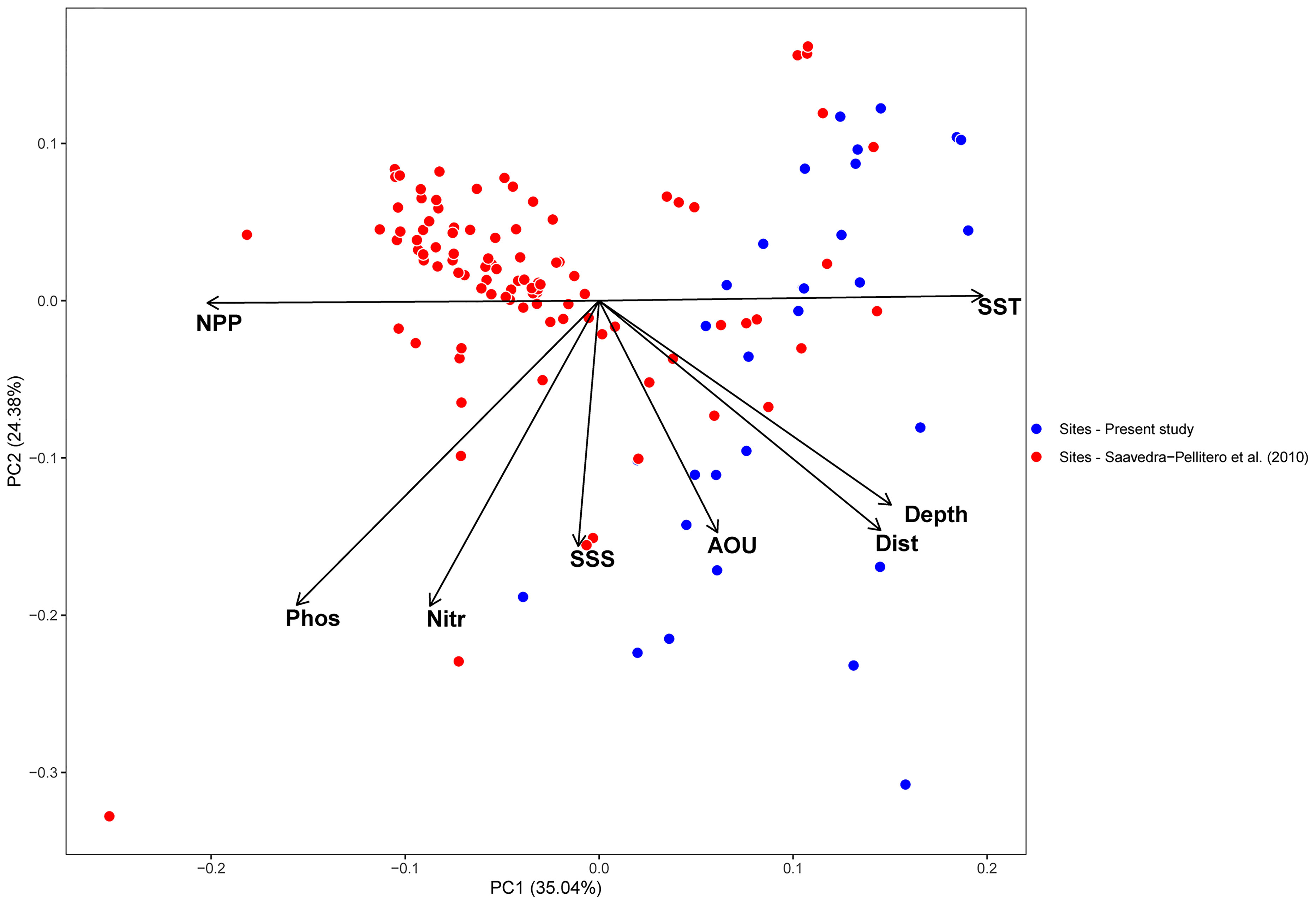
Figure 3 Principal component analysis (PCA) of the environmental dataset. The red and blue dots correspond to the scores of the samples from Saavedra-Pellitero et al. (2010) and the present study, respectively. AOU=apparent oxygen utilization, Depth = sample depth, Dist. = distance to the coast, NPP = annual averaged Net Primary Productivity, Nitr = annual averaged nitrate content at 10 m water depth, Phos = annual averaged phosphate content at 10 m, SSS = annual averaged sea surface salinity at 10 m and SST = annual averaged sea surface temperature at 10 m.

The RDA shows that there is large compositional difference between the coccolith assemblages from the new dataset and from Saavedra-Pellitero et al. (2010) (Figure 4). However, despite sampling across larger environmental gradients, the species-environment response remains linear (DCA1: 1.25 SD). The variance explained by the environmental variables included in the RDA is ca. 36%. The samples analysed in this study are located in the left side of the ordination plot, related to higher SSTa. Species such as G. oceanica, Oolithotus sp., Umbilicosphaera spp., and F. profunda appear related to these higher SSTa, whilst G. muellerae, E. huxleyi, C. leptoporus, and C. pelagicus appear on the right side of the RDA plot, characterized by lower SSTa and higher NPP values (Figure 4). The ratio between the first constrained axis (RDA1) and the first unconstrained axis (PC1) is the highest for SSTa (1.5), indicating that this variable should be the one used in the model. SSTa explains more than 15% of the coccolith species-environment variation.

FIGURE 4

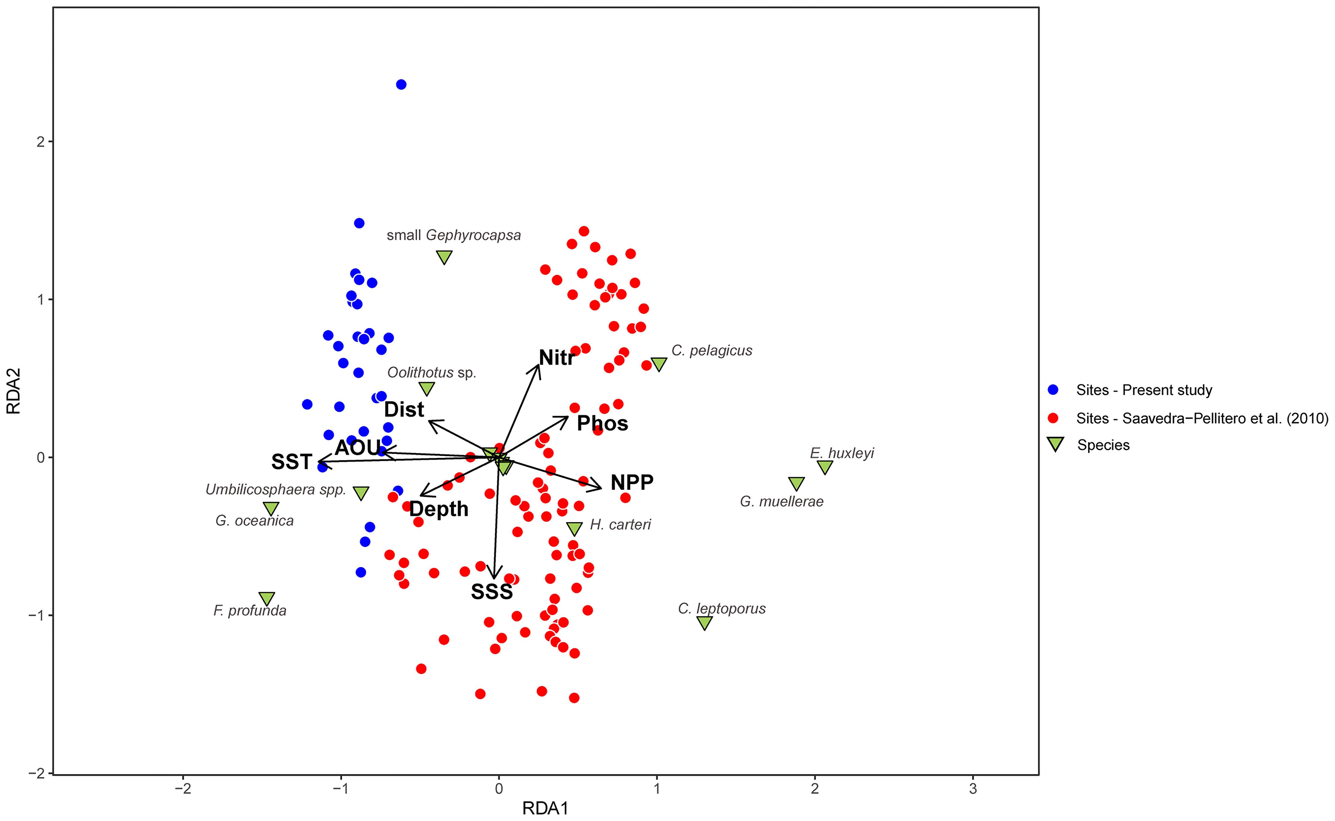
Figure 4 Redundancy Analysis (RDA) biplot showing the sample scores in red (Saavedra-Pellitero et al., 2010) and blue (present study), and the species scores in green. AOU=apparent oxygen utilization, Depth = sample depth, Dist. = distance to the coast, NPP = annual averaged Net Primary Productivity, Nitr = annual averaged nitrate content at 10 m water depth, Phos = annual averaged phosphate content at 10 m, SSS = annual averaged sea surface salinity at 10 m and SST = annual averaged sea surface temperature at 10 m.

The lineal species-environment response and the thermal tolerances of the coccolithophore species indicate that some of the taxa, such as small Gephyrocapsa, show similar abundances across a SSTa range of almost ~20°C (Figure 5). Species such as E. huxleyi, G. muellerae, C. leptoporus and Helicosphaera carteri show higher abundances at SSTa below 20°C, although they do not indicate a uniform increase with decreasing temperatures. Other species show a clearer response to changes in SSTa, including increased abundances of Florisphaera profunda above 14°C, and of C. pelagicus below 13°C. Other taxa show potential thermal niches in the SEP and EEP, ranging 12-17°C for Pontosphaera spp., and 17-20°C for Calciosolenia sp. However, the taxa which show more defined SSTs are not as abundant as taxa with higher ecological plasticity, such as those from the genus Gephyrocapsa.

FIGURE 5

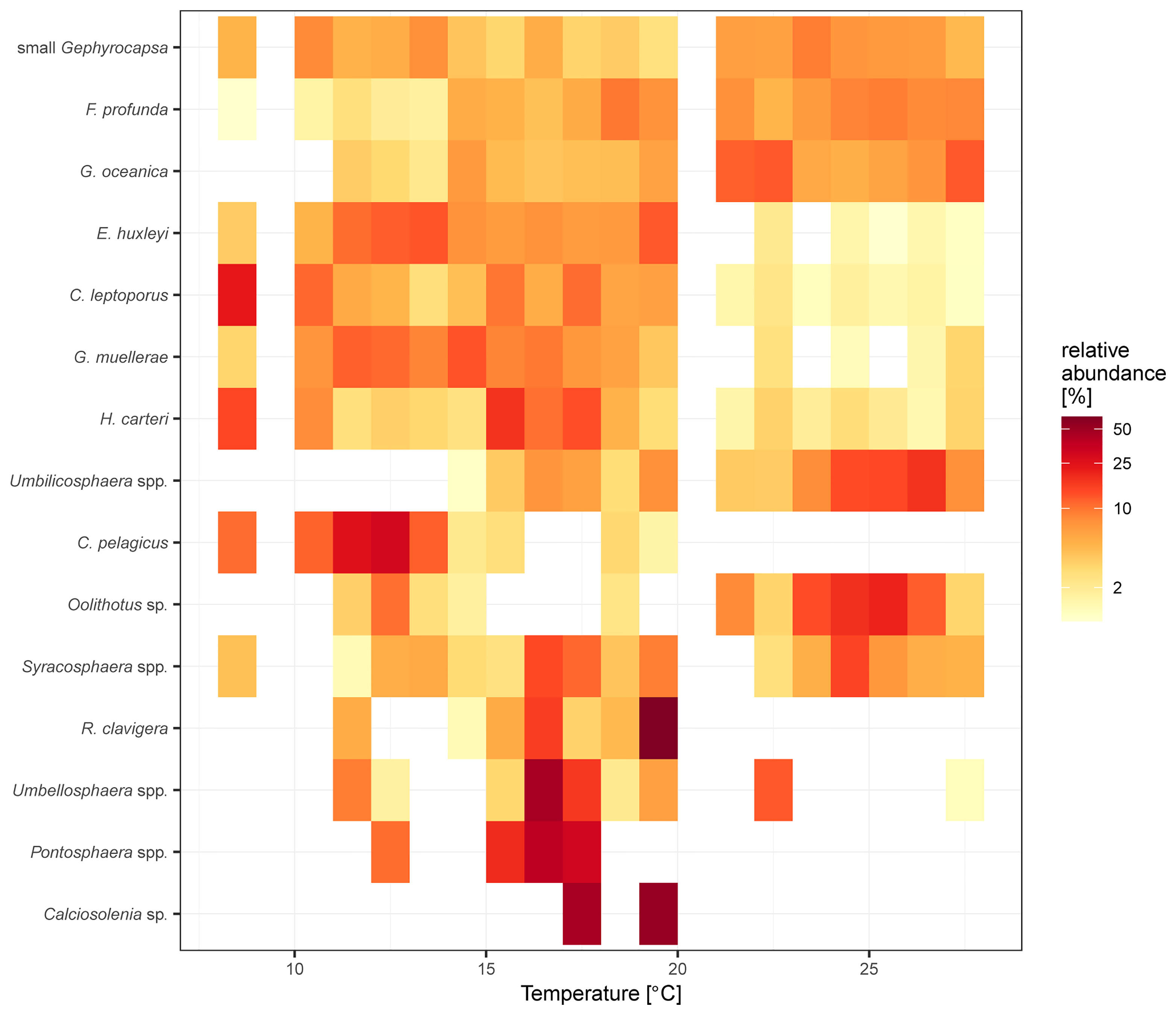
Figure 5 Coccolithophore species thermal niche for surface sediment samples from Saavedra-Pellitero et al. (2010) and the present study. Colors indicate average relative abundance within 1°C bins. Note the gaps at 9-10°C and between 20-21°C, due to the lack of samples covering those specific SSTa ranges.

4.3 Coccolith-Based SSTa Model

For the coccolith-temperature based regression, we applied the R² of the final model using IKFA regression with 2-factors (assessed using a screeplot) - 0.82 - with an RMSEP of 2.4°C (Figure 6A). There are only minor gaps in the SSTa gradient (9-10°C and 20-21°C) due to absence of surface sediment samples covering these SSTa values in the modern calibration dataset. Interestingly, the fitting line for the EEP (SSTa range between 28-20°C) samples from Saavedra-Pellitero et al. (2010) shows a different slope than the 1:1 line, while the predicted temperatures based on the new EEP surface samples in this study show a better fit to the observed values. No outliers, as defined as residuals higher than 2 * SD the SSTa at 10 m, were identified (Figure 6B).

FIGURE 6

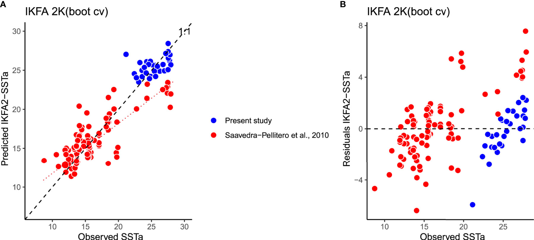
Figure 6 (A) Observed versus Predicted annual SSTa at 10 m using coccolith assemblages from the surface sediments in samples from Saavedra-Pellitero et al. (2010) (red) and the present study (blue), using a Imbrie-Kipp factor analysis (IKFA) with 2 factors, under bootstrapping cross-validation (999 iterations). (B) Residual versus Observed annual SSTa at 10 m. Dashed line in (A) indicates the regression line between all the observed vs predicted SSTs, and dotted line just considering Saavedra-Pellitero et al. (2010).

4.4 Florisphaera profunda-Based NPP Model

For the F. profunda-NPP regression, we added 32 new samples from the EEP to the global regression made by Hernández-Almeida et al. (2019) (Figure 7). These new data fits well with the previous F. profunda-NPP regression (see blue dots in Figure 7), and the new determination coefficient of this model (R² = 0.52, standard error = 1.02 mg C m^-2 day^-1) does not differ significantly from that originally published (R² = 0.54). It is important to note that the new samples show a better fit to the regression line compared to EEP samples from Saavedra-Pellitero et al. (2011).

FIGURE 7

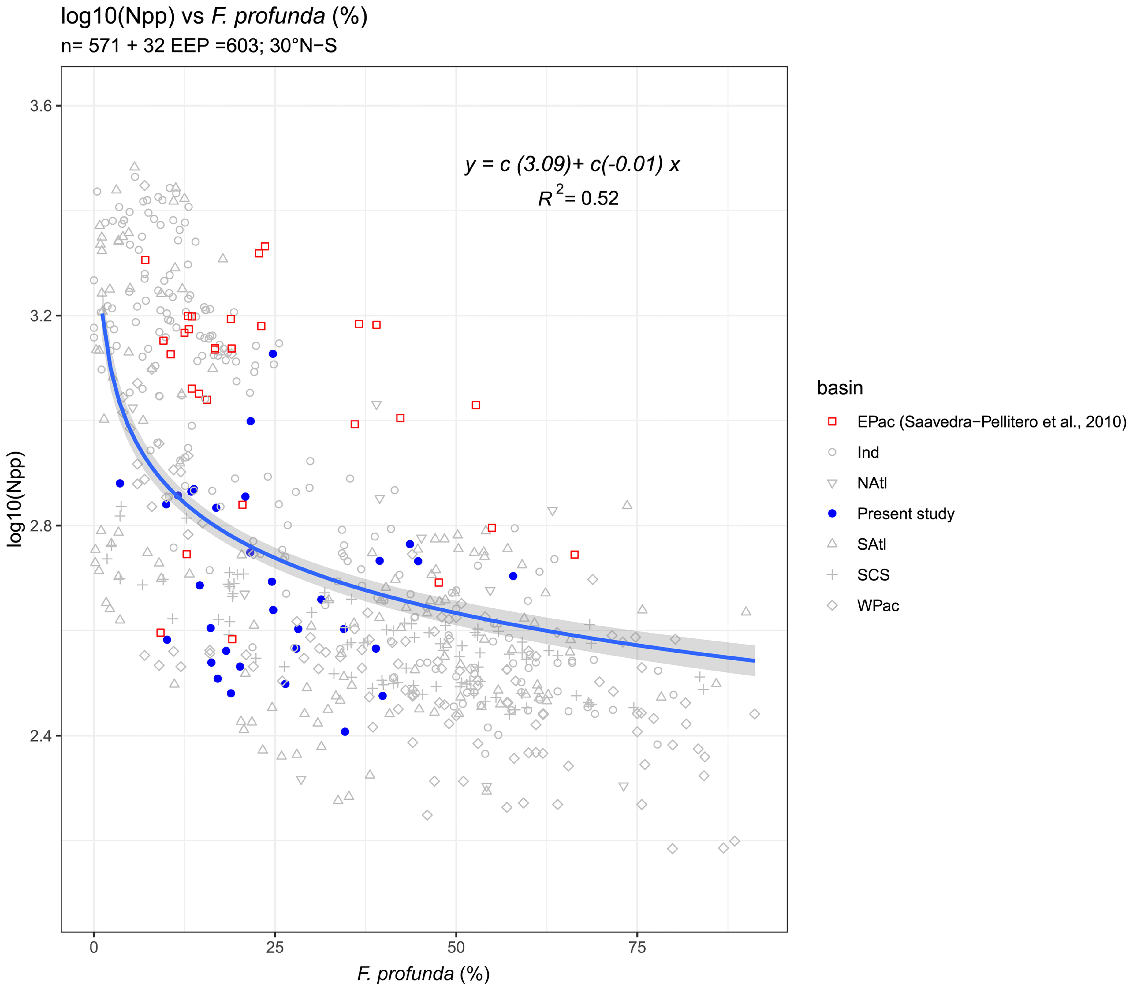
Figure 7 Regression between relative abundance of Florisphaera profunda in surface sediments located between 30°N-30°S in different basins across the World’s oceans and NPP (in mg C m^-2 day^-1) from VGPM estimates for the same locations (Hernández-Almeida et al., 2019) indicated with a blue line. The regression includes samples from Saavedra-Pellitero et al. (2010) located in the Eastern Pacific (EPac, indicated with red squares). The blue dots represent the F. profunda-NPP relationship for the new surface sediment samples from this study, located in the Eastern Equatorial Pacific and the grey shaded area shows the residual standard error (0.63).

4.5 Downcore Coccolith Assemblage, Abundance and Preservation

Coccolith CEX’ values at ODP Site 1240 are in general above 0.9 suggesting moderate to good preservation (Figure 8J). CEX’ values are below 0.9 only at the beginning of Termination I, between ~19 and ~17.5 kyr, due to an increase in the relative abundance of C. leptoporus probably due to low SSTs, and perhaps to preservation (not obvious in light microscope observations). The sub-fossil coccolithophore taxa preserved in the surface sediment samples are also present in the section studied. The downcore assemblage is dominated by small Gephyrocapsa, G. oceanica, and F. profunda. Small Gephyrocapsa ranges between 18.4% and 52.5% (mean of 37.5%) and is present in low abundance at the beginning of Termination I, with a marked increase between 17.5 to 16.5 kyr. High percentages of small Gephyrocapsa are recorded between 16.5 to 15.5 kyr, around 14.5 kyr, and between 13.5 and 12 kyr, followed by a relatively gradual decrease after 13 ka. Gephyrocapsa oceanica makes up a mean relative abundance of 26.4%, and varies from 10.3% to 50.9%. This species is more abundant at the beginning of Termination I with marked drops between 17.5 – 17 kyr and during the warm Bølling–Allerød (BA) period, from 14.7 to 12.9 kyr. Lower percentages (ca. 20%) of G. oceanica are observed during the Holocene, with an occasional increase at around 5.5 ka. Florisphaera profunda is an abundant taxon which varies from 7.7% to 45%, and shows increasing values from the beginning of the studied interval towards present times. The coccolith assemblage is dominated by F. profunda during most of the Holocene.

FIGURE 8

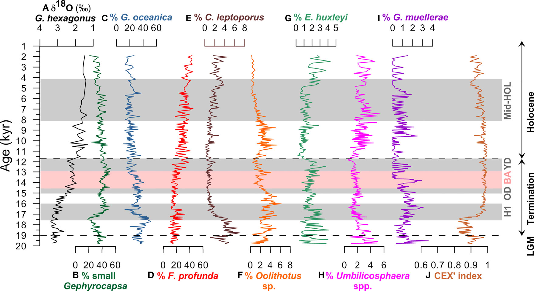
Figure 8 (A) Downcore δ¹⁸O (‰) record from the planktonic foraminifera Globorotaloides hexagonus (Max et al., 2017; Rippert et al., 2017), relative abundances of the most important coccolithophore species (>1% on average): (B) small Gephyrocapsa, (C) Gephyrocapsa oceanica, (D) Florisphaera profunda, (E) Calcidiscus leptoporus, (F) Oolithotus sp., (G) Emiliania huxleyi, (H) Umbilicosphaera spp., (I) Gephyrocapsa muellerae, and (J) CEX’ at ODP Site 1240 between 20-1.9 kyr. Shaded areas indicate the Heinrich 1 (H1), Older Dryas (OD), Bølling–Allerød (BA) and Younger Dryas (YD) time intervals. Dashed lines indicate the limits between the Last Glacial Maximum (LGM)-Termination I, and Termination I-Holocene.

Other taxa are subordinate, with low relative abundances of G. muellerae recorded during Termination I (near 3%), and marked increases around 16.5 and 14 kyr, although relative abundances remained below 1% for many intervals of the studied period. Emiliania huxleyi fluctuates throughout the sedimentary sequence, reaching a maximum abundance of 4.3% around 2.5 ka, and lowest abundance between 11.5 – 5 kyr. The relative abundance of C. leptoporus is highest at the beginning of Termination I, especially from ca. 20 – 17 kyr (reaching a maximum of 6.9%), and during the late Holocene. Umbilicosphaera spp. reaches relatively high relative abundance before the BA and during the Holocene, up to 5.3%, and has low values between 17 – 11 kyr. The total CAR showed maximum values during Termination I with a marked decrease at the end of the YD (Figure 10A). Increased CAR values were recorded from ca. 10.5 to 5 kyr, and the lowest values during the Holocene, from ca 4.5 to 1.9 kyr.

4.6 Temperature and Productivity Reconstructions

We applied the new IKFA-2 calibration model to the downcore coccolithophore assemblages at ODP Site 1240 to reconstruct SSTa (Figure 9). Estimated SSTa vary between ~20.7 and 25.4°C for the last ~20 kyr, with the lowest values recorded at ~19.8 kyr, during the LGM, and highest at the beginning of the Holocene, at ~10.5 ka (Figure 9C). The SST change across the Termination goes from 22.4 to 25.4°C at the highest warming, which is above the calibration error (2.4°C). Other thermal oscillations of smaller magnitude have to be taken with caution, because they are within the magnitude error. A drop in SSTa coincident with the Antarctic Cold reversal, an Antarctic cooling event which started at 14.5 and lasted ca. two millennia (Blunier et al., 1997) is recorded during Termination I, from ~14.7 to ~11.4 kyr. From the beginning of the Holocene towards modern times (i.e., 1.9 kyr), SSTa fluctuate, but generally decrease (Figure 9). The squared chord distance of the nearest analogue from the modern dataset in this study to each fossil sample for Site 1240 is shown in Supplementary Figure S1A, and “good” analogues could be identified among the modern samples for the fossil assemblages. The analyses for the significance of the environmental variables in the downcore data shows that the fossil assemblage at Site 1240 is driven by SSTa (p<0.05) (Supplementary Figure S1B).

FIGURE 9

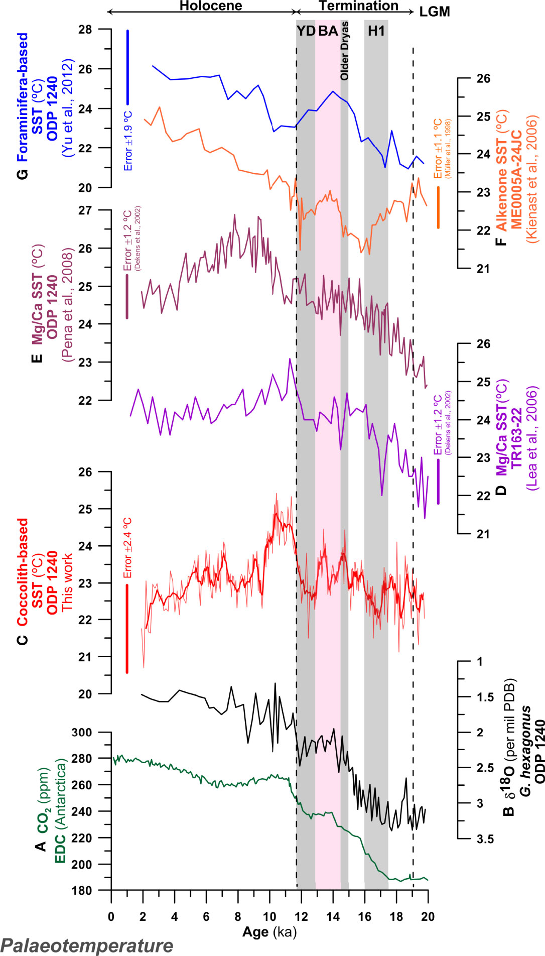
Figure 9 Palaeotemperature records for the last 20 kyr in eastern equatorial Pacific Ocean. (A) CO₂ (ppm) EDC (Luthi et al., 2008); (B) δ¹⁸O (‰) record from the planktonic foraminifera Globorotaloides hexagonus at ODP Site 1240 (Max et al., 2017; Rippert et al., 2017); (C) coccolith-derived sea surface temperature SSTa, (°C) at ODP Site 1240 (this work) with 5-point running average smoothing; (D) SSTs (°C) based on Mg/Ca from Globigerinoides ruber in the core TR-163-22 (Lea et al., 2006); (E) SSTs (°C) based on Mg/Ca in G. ruber at ODP Site 1240 (Pena et al., 2008); (F) alkenone-derived sea SSTs (°C) from core ME0005A-24JC (Kienast et al., 2006); (G) Foraminifera-derived SSTs (°C) at ODP Site 1240 (Yu et al., 2012). Shaded areas indicate the Heinrich 1 (H1), Older Dryas, Bølling–Allerød (BA) and Younger Dryas (YD). Vertical bars indicate the error estimated for the different SST proxies; Müller et al. (1998) was used for alkenones and Dekens et al. (2002) for Mg/Ca.

Estimated palaeoproductivity based on the global calibration of the relative abundance of F. profunda (Hernández-Almeida et al., 2019) varies between ~448.2 and 1071.6 mg C m^-2 day^-1 ( ± 1.02 mg C m^-2 day^-1) for the last ~20 kyr. Highest NPP values are recorded prior to 17 kyr, while low NPP occurs during mid to late Holocene (Figure 10). The reconstructed NPP shows variations with a clear gradual decreasing trend for the last ~20 kyr (Figure 10), punctuated by two troughs at 17 and 12 ka.

FIGURE 10

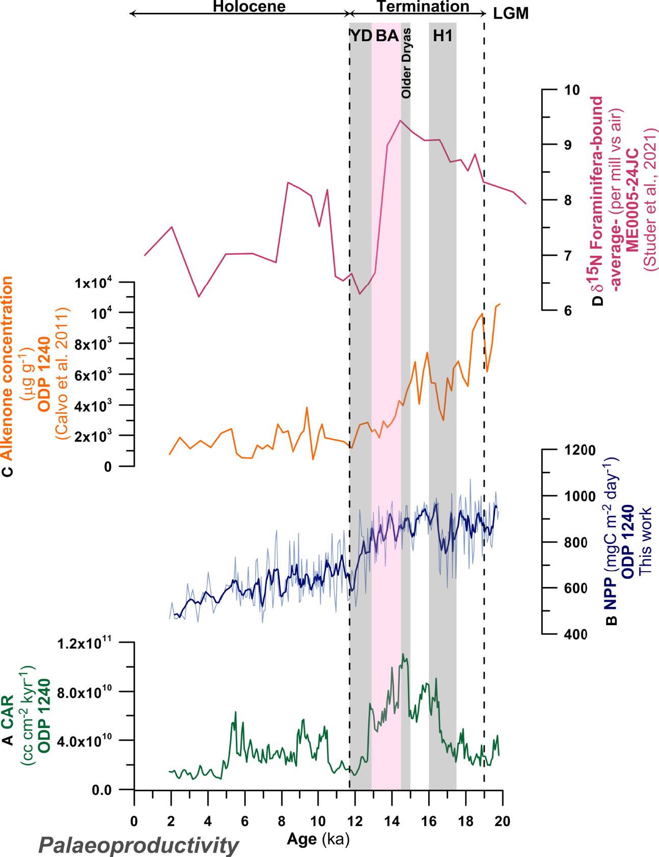
Figure 10 Palaeoproductivity records for the last 20 kyr in eastern equatorial Pacific Ocean. Left panel: (A) Coccolith accumulation rate (CAR, cc cm^-2 kyr^-1) at ODP Site 1240; (B) coccolith-derived Net Primary Productivity (NPP, mg C m^-2 day^-1) at ODP Site 1240 (this work) including error estimates and with a 5-point running average smoothing; (C) alkenone concentration (µg g^-1) at ODP Site 1240 (Calvo et al., 2011); (D) Foraminifera-bound δ¹⁵N (‰ vs air) (average of Neogloboquadrina dutertrei and N. incompta) (Studer et al., 2021). Shaded areas indicate the Heinrich 1 (H1), Older Dryas, Bølling–Allerød (BA) and Younger Dryas (YD).

5 Discussion

Strong and dynamic changes in temperature and primary productivity occur across the EEP in response to recent major climate Pleistocene-Holocene transitions (e.g., Dubois et al., 2009; Kienast et al., 2013; Costa et al., 2017; Ford et al., 2018). However, conflicting SST and NPP reconstructions through Termination I and the Holocene may reflect real variability in the EEP or might be artifacts of the different proxies and techniques used in various studies (Costa et al., 2017). Almost all proxies are susceptible to seasonal or water depth habitat biases (e.g., Mix, 2006; Dubois et al., 2009; Leduc et al., 2010; Timmermann et al., 2014), but considering these as part of a multiproxy study, alongside the coccolithophore-based approaches presented here, allows a more nuanced assessment of past productivity and temperature variability. Our new models for SSTa and NPP are used to generate a high-resolution reconstruction of oceanographic conditions at ODP Site 1240 over the last 20 kyr.

Assessment of our new IKFA-2 coccolith-based SSTa calibration model shows a better performance (R² = 0.82, RMSEP = 2.4) compared to the previous coccolithophore-based transfer functions to reconstruct SST in the EEP (Saavedra-Pellitero et al., 2011; Saavedra-Pellitero et al., 2013) (R² = 0.57 -not cross-validated-; R² = 0.702, RMSEP = 0.803 -cross validated-, respectively). The samples at locations with SST >22°C in the previous calibration model of Saavedra-Pellitero et al. (2011) fall below the 1:1 line in the observed vs predicted SST (dotted line in Figure 6A), systematically underestimating SSTs. This trend could be due to the fact that the old approach of Saavedra-Pellitero et al. (2011) was based on Principal Component Analysis and the main factor dominating in the EEP was not considered for the palaeoenvironmental reconstruction. That factor (Factor 1) explained 31.58% of the variance, was correlated with silicate content and SST and dominated by the species F. profunda and G. oceanica. Most likely, the temperature underestimates could be due to the use of G. oceanica in the model, which shows similar abundances across a SSTa range of almost ~20°C in the SEP and EEP (Figure 5). Regarding the follow-up model of Saavedra-Pellitero et al. (2013), low latitude surface sediment samples were excluded in that calibration, therefore the SST range was narrower than in this work and the potential for reconstructions became reduced and restricted just to the SEP. With the addition of the surface sediment samples analyzed in this study, the slope of the predicted versus observed SSTa new model has a value ca. 1 (Figure 6A), which leads to a more robust calibration in the EEP and allows the model’s application to fossil coccolithophore records in the Eastern Pacific, from the Equator to Southern mid-latitudes (ca. 47˚S), with increased confidence.

5.1 SSTa Reconstruction at ODP Site 1240

5.1.1 Termination I

All planktonic foraminiferal-based proxies at ODP Site 1240 show a trend of more-or-less consistent warming through the last Termination of ~4°C (Lea et al., 2006; Pena et al., 2008; Yu et al., 2012) (Figures 9B, D, E, G). This pattern of warming contrasts with coccolithophore-derived, alkenone-based SST (UK’₃₇) estimates from core ME0005A-24JC (0°01′N, 86°27′W, 2941 m depth) (Kienast et al., 2006), that show a distinct ~1.5°C cooling between ~18 and 15 kyr, before warming a similar amount by the BA/Younger Dryas (YD) (Figure 9F). Interestingly, our new assemblage-based SST estimates (Figure 9C) show an intermediate behavior, with cycles of warming and cooling of magnitudes <1.5°C through the Termination but with only a small long-term background warming trend across the whole Termination. Particular cool intervals are associated with Heinrich 1 (H1) and the YD and, in this, most closely resemble the planktonic foraminiferal Mg/Ca records from the nearby Site TR-163-22 (0°3′N, 92°23′W, 2830 m water depth, Figure 9D) (Lea et al., 2006). We speculate that these patterns could suggest certain degree of seasonal or inter-annual offset between the bloom-forming alkenone-producers, mainly Gephyrocapsa species in this instance, and the wider and phylogenetically more diverse community that contributes to the warmer assemblage-based SSTs (such as Oolithotus sp., Umbilicosphaera spp. and F. profunda; see Figure 5). Additionally, Kienast et al. (2006) suggest that the ENSO-related dynamics could have an overprint on the alkenone-based SST record in the EEP. The offsets between alkenone and assemblage-based SSTs are most marked in the interval between H1 and the Older Dryas (15 – 16 kyrs), where alkenone-production appears to be in waters ~1.5°C cooler than the temperatures indicated by the whole assemblage.

Increasing seasonality of production through the Termination could also explain the increasing offset between foraminiferal- and coccolithophore-derived SSTs, if algal production was biased towards early upwelling of cold-tongue waters as have been ascribed in the EEP and elsewhere (e.g., Kienast et al., 2006; Leduc et al., 2010; Schneider et al., 2010; Timmermann et al., 2014). For example, foraminifera-based Mg/Ca-data potentially reflects boreal summer insolation changes, as shown by present-day G. ruber fluxes in the Panama Basin (Thunell et al., 1983; Leduc et al., 2010), whilst coccolithophore-derived alkenone SSTs reflecting a bias towards boreal winter temperatures (Timmermann et al., 2014). Taken together, this data indicates seasonal warming of boreal winters through Termination I, but with the persistent presence of colder upwelling waters, with a boreal winter or even Southern Hemisphere-sourced temperature signal (Martínez-Botí et al., 2015; Diz et al., 2018).

5.1.2 Holocene SSTs

Foraminiferal Mg/Ca temperatures from both ODP Site 1240 and core TR-163-22 reach peak temperatures in the early Holocene (~ 6 to 10 kyr), before either cooling slightly and stabilizing (TR-163-22, Figure 9D) or cooling to almost the Recent (ODP 1240) (Figure 9E). The discrepancies between both Mg/Ca SST records from near-by locations are attributed to the differential impacts of dissolution between the sites (e.g., Mekik et al., 2007; Dubois et al., 2009; Leduc et al., 2010), with foraminiferal preservation getting worse during late Holocene at core TR-163-22 (Lea et al., 2006). In contrast, alkenone-based SST records warm by almost 2°C through the Holocene (Figure 9F), but only so as to converge on the warmer (~24 – 25°C) Mg/Ca SSTs in the late Holocene. Foraminiferal assemblage SSTs (Figure 9G) are also consistently warm through the Holocene, but are ~2°C warmer than the alkenone SSTs. Again, these patterns suggests a warm-season/boreal signal recorded within the G. ruber Mg/Ca data, whilst alkenone (and foraminiferal assemblage data) track the temperature trends of Southern Ocean-derived upwelling waters. The coccolithophore assemblage-based signal (Figure 9C) thereby tracks the Mg/Ca data more closely, with a general slight cooling through the Holocene, but with the coolest late-Holocene temperatures of any of the proxies. These trends indicate a long-term warm-season (G. ruber-like) behavior but with a potential cool-bias in the modern calibration data, as indicated by latest Holocene/pre-industrial SST estimates of ~22 – 23°C against measured mean annual temperatures at this location of ~24.5°C.

5.2 Productivity Reconstruction at ODP Site 1240

In the same way that SST records can vary according to the different proxy sensitivities (Figure 9), conflicting EEP productivity reconstructions for the last 20 kyr may reflect real variability or be artifacts of the proxy techniques used (Costa et al., 2017). Combining a range of proxies responsive to productivity provides a better understanding of the interaction between nutrient availability, consumption and NPP in the surface ocean, its transport in the water column and burial in the sea-floor.

5.2.1 Termination I

While alkenone concentration (Calvo et al., 2011) at ODP Site 1240 (Figure 10C), show high values during the LGM and gradually decrease during Termination I, F. profunda-based NPP (Figure 10B) is fairly consistent from LGM to mid-BA, when it starts to decline. The general declining trend is also observed in reconstructed NPP at low resolution at ODP 677B (1.28°N; 83.748°W, 3461 m depth; Martínez et al., 2006) and RC13-110 (0.097°S, 95.653°W, 3231 m depth; Beaufort et al., 2001) using the calibration of Hernández-Almeida et al. (2019) (Figures S2A, C). The NPP-F.profunda in MD02-2529 (8.208° N, 84.125° W, 1619 m depth; Ivanova et al., 2012), however, shows an increase from the LGM to the YD, which then only slowly declines through the Holocene (Figure S2D). The NPP-F.profunda data, CAR and alkenone concentration at ODP Site 1240 show a significant up swing through the end of H1 and persisting the trough the BA (alkenone accumulation) or YD (NPP-F.profunda and CAR) (Figures 10A–C). Using CAR as a coccolithophore productivity proxy assumes that there is no preservation (carbonate dissolution) and/or dilution bias, in our case supported by high CEX’ values (Figure 8). Both, Anderson et al. (2019) and Jacobel et al. (2020), using different sensitive redox proxies, determined that higher alkenone concentration record prior to the Holocene and deglaciation are the result of changes in bottom water oxygenation at Site 1240. These and other studies in the Pacific Ocean observed enhanced alkenone preservation during poor oxygenation conditions, indicating that alkenone abundance at ODP Site 1240 could be controlled as much by preservation as by primary productivity (Anderson et al., 2019). Although this may account for some of the decline and its dynamics between the LGM and Holocene, the timing of the increase in alkenone accumulation, coincident with other proxies at the end of H1, implies a strong primary signal from increased coccolithophore production at H1. This pattern of coccolithophore productivity increase through H1 to YD is also more consistent with the NPP-F.profunda records from MD02-2529, which peak during the same interval (Figure S2).

The relatively high primary phytoplankton production from H1 to YD (with estimated NPP values ranging from ca. 1000 to 700 mg C m^-2 day^-1, Figure 1H) is consistent with a broad peak in ²³⁰Th normalized organic carbon burial flux at ME0005A-24JC (a site survey core for ODP Site 1240) (Figure 11D). Even though Kienast et al. (2006) proposed that high palaeoproductivity was fueled by coastal upwelling during those intervals, the records presented here suggest that increased primary production in the EEP phytoplankton community and associated increased organic carbon export was also a strong feature of this interval.

FIGURE 11

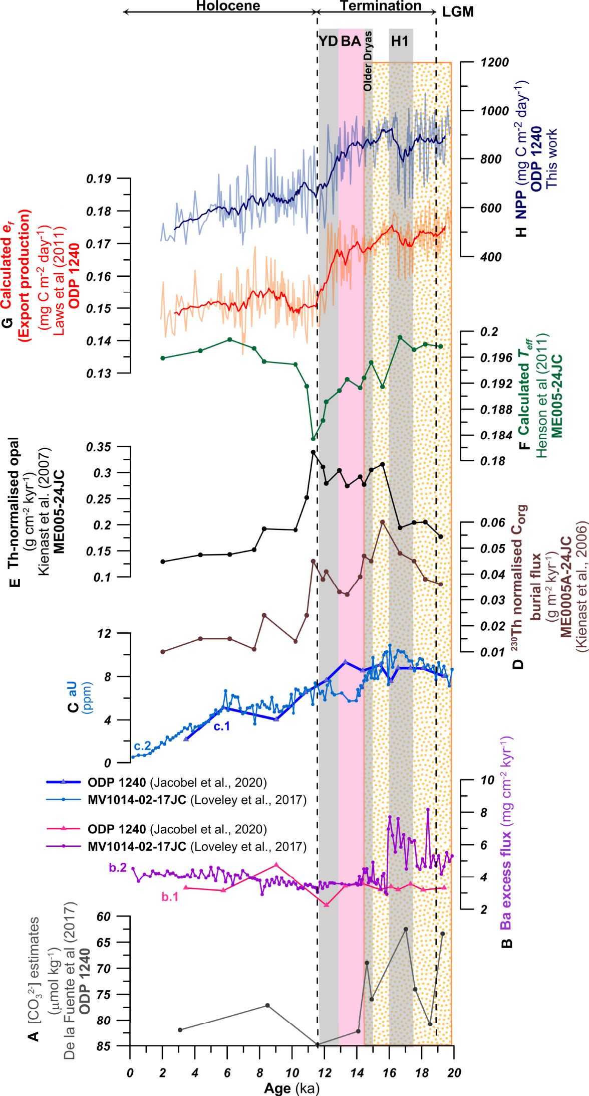
Figure 11 Variations in the components of the biological pump since the late LGM at ODP Site 1240 and ME0005A-24JC. (A) $\left[{\text{CO}}_3^{2-}\right]$ estimates (µmol kg^-1) (de la Fuente et al., 2017) -note the inverted scale-, (B) b.1: Ba excess flux (mg cm^-2 ka^-1) at ODP Site 1240 –triangles- (Jacobel et al., 2020) and b.2: Ba excess flux (mg cm^-2 ka^-1) at MV101402-17JC –dots- (Loveley et al., 2017); (C) c.1: authigenic uranium (aU, in ppm) at ODP Site 1240 –triangles- (Jacobel et al., 2020) and c.2: aU (in ppm) at MV101402-17JC –dots- (Loveley et al., 2017); (D) ²³⁰Th-normalized organic carbon burial flux at ME0005A-24JC (g m^-2 yr^-1) (Kienast et al., 2006); (E) ²³⁰Th-normalized opal flux (g m^-2 yr^-1) (Kienast et al., 2007); (F) Calculated transfer efficiency (T_eff) following Henson et al. (2012); (G) calculated export production (e_f) using equation 5 (mg C m^-2 day^-1) following Laws et al. (2011) and with 13-point running average smoothing; (H) F. profunda-derived NPP (mg C m^-2 day^-1, this work with 13-point running average smoothing). Black dashed lines indicate the late LGM, Termination I and the Holocene. Shaded areas indicate the Heinrich 1 (H1), Older Dryas, Bølling–Allerød (BA) and Younger Dryas (YD). The orange dotted interval highlights high NPP and export production, and low oxygenation of the deep-ocean.

Ba fluxes, an inorganic productivity proxy for carbon rain, have been also measured at ODP Site 1240 (Jacobel et al., 2020) (Figure 11B b.1), but at a much lower resolution than our NPP record, which makes comparison complicated. At Site MV1014-02-17JC (0.18°S, 85.86°W), however, Ba fluxes show a step-change at H1 (Figure 11B b.2), more than halving from high LGM values, which broadly correlates with the increase in coccolithophore productivity indices at ODP Site 1240 (NPP-F.profunda, CAR and alkenone accumulation, Figure 10) and a marked rise in Th-normalized opal accumulation, which is another proxy for carbon flux at ME005-24JC (Figure 11E). Together, these clearly show a switch in productivity and export production regimes, with an increase in calcareous phytoplankton productivity, as well as in opal export, but a marked decline in excess Ba flux. These combined signals are potentially indicative of increased ventilation of sub-thermocline water together with increase nutrient upwelling to the mixed-layer, stimulating phytoplankton production but markedly reducing Ba export. It is worth noting that this is also the start of the decoupling between CAR and NPP-F. profunda (carbonate-based proxies) and alkenone accumulation rates (organic proxy) (Figure 10) and the start of a decline in ²³⁰Th normalized organic carbon burial flux (Figure 11D). Again, this all suggests a decoupling between the export efficiency of organic carbon and carbonate through the Termination, whilst primary production remained high.

Foraminifera bound δ¹⁵N (¹⁵N/¹⁴N ratio, a proxy for water-column denitrification) measured on Neogloboquadrina dutertrei and N. incompta (average values in Figure 10D) at ME0005A-24JC, show higher values up to the BA suddenly dropping during the YD (Studer et al., 2021). This pattern shows similarities with our CAR and NPP-F.profunda reconstructions, which drop at the end of Termination I (Figures 10A, B). Studer et al. (2021) suggests that planktonic foraminifera δ¹⁵N could be driven by changes in the δ¹⁵N in intermediate water, nitrogen advection and nitrogen utilization by the phytoplankton, on top of the previously inferred δ¹⁵N reduction in water column denitrification during the glacial suggested by Dubois and Kienast (2011) -based on bulk measurements-. The nitrogen utilization by phytoplankton as an explanation for part of the δ¹⁵N variability is supported by our F. profunda-based data, with high steady NPP during Termination I (up to the BA) and a lower values during the Holocene.

5.2.2 Holocene

Almost all of the productivity indicators we considered here are consistent in reconstructing substantially lower Holocene primary productivity and export than that through either the LGM or the Termination, with a long-term trend of decline towards 1.9 ka. There is, however, a broad distinction between those related to organic carbon export and burial (alkenone accumulation, ²³⁰Th normalized organic carbon burial flux, Ba excess flux and Th-normalized opal accumulation) which all decline markedly either through or sharply at the end of Termination I (Figure 10C and Figures 11B, D, E), and primary productivity proxies based on coccolithophore assemblages or accumulation rates that decrease more steadily through the Holocene (Figures 10A, B). In some instances, in proxies such as our CAR record at ODP Site 1240, there are actual transient increases in the early Holocene, with moderate values persisting through the mid Holocene. By the last 5 kyr, however, even CAR has reached a minimum for the entire record. As with the discussion above for the LGM to Termination interval, this indicates either a decoupling between primary production and organic carbon export efficiency, with the former declining more slowly in the early Holocene, or a potential shift in nutrient regimes that impacted siliceous primary production and organic carbon export at the end of the Termination, but that had less of an impact on the calcareous phytoplankton, which, instead, experienced a more gradual decline in productivity through the Holocene.

5.3 Implications for the Export Productivity at ODP Site 1240

In order to better understand the fate of the plankton primary production sinking throughout the water column, we calculated the ratio of export production to total NPP (e_f) at ODP Site 1240 (Equation 5 in this paper) following Laws et al. (2011). For this, we combined our estimates of NPP and SSTa. The reconstructed e_f (Figure 11G) shows a pattern with higher export during the LGM and throughout Termination I, which decreases rapidly at the start of the Holocene, followed by a small increase between 9-5 kyr, to decrease again towards the most recent times. The high glacial e_f is followed by a rapid decrease from the BA to the beginning of the Holocene. This rapid decrease in e_f is also observed in the transfer efficiency (T_eff) (Figure 11F), calculated using Th-normalized opal and CaCO₃ fluxes at ME0005-24JC.

We interpret the higher e_f values during LGM and the deglaciation (Figure 11G) as a rise in nutrient supply to the thermocline, as noted by the higher δ¹⁵N in planktonic foraminifera (N. dutertrei and N. incompta) (Studer et al., 2021) (Figure 10D), which resulted in higher NPP and export production (Costa et al., 2017; Jacobel et al., 2020). The lower SST during this interval prevented high remineralization of the organic detritus in the photic zone, leading to a more efficient downward transport of organic detritus and burial in the sea-floor (Henson et al., 2012). This higher e_f during the LGM and Termination I indicates that the productivity at the EEP contributed actively to decrease the atmospheric CO₂ levels (Figure 9A), as it was suggested by other studies (e.g., de la Fuente et al., 2017).

The coupled decrease in productivity, e_f and T_eff during the end of Termination I and the beginning of the Holocene (Figures 11F, G, H) contrasts with the elevated biogenic opal and organic Carbon fluxes (Figures 11D, E) at that time. The increased opal productivity between 15-11 kyr has been explained by a higher influence of Si-rich waters from the Southern Ocean transported to the Equator, which stimulated diatom productivity with respect to coccolithophore productivity during the deglaciation (Calvo et al., 2011). It is important to note that the change in ecosystem structure, from calcareous to siliceous plankton, and expected reduction in the carbonate pump (lower calcareous productivity), was not translated into a more efficient export production, as seen by the decrease in T_eff (Figure 11F). A potential explanation for this is the ‘packaging effect’ (Francois et al., 2002) associated with the shift in the floral community, in which fast-sinking fecal pellets are produced in carbonate-dominated environments, while opal-dominated regions are characterized by very loose aggregates that may sink slower and can be more readily remineralized, reducing the T_eff (Henson et al., 2011). Another alternative explanation for the higher opal content, not matching the NPP and e_f reconstructions, would be that between 16-9 ka sedimentation rates are higher at site ME0005-24. Faster burial could lead to better preservation of biogenic opal in the sediment (Kienast et al., 2007). Calcium carbonate dissolution has been observed in different Late Pleistocene records of the EEP (e.g., Ivanova et al., 2012; Diz et al., 2018), and would be a mechanism to explain the increase in opal at ME0005A-24JC and decrease in carbonate-based productivity indicators (NPP and CaCO₃%) between 15-11 kyr. However, good to moderate coccolith preservation has been observed at ODP Site 1240 for the last seven glacial cycles (López-Otálvaro et al., 2008), which is supported by the low CEX’ values calculated for our study (Figure 8J). This suggests that the lysocline was located below 2900 m at Site 1240 for the last ca. 20 kyr. Consequently, we hypothesize that the decoupling between estimates of NPP and e_f based on calcareous proxies and % opal is a combined result of shifts in plankton community forced by hydrographic factors, and the better preservation of opal during intervals of higher sedimentation rates in the EEP.

Our records showing higher NPP, e_f and T_eff during the last part of the LGM and H1 compared to the Holocene, interpreted as a decrease in export production, do not agree with the reconstruction of organic carbon rain at Site 1240 using Th-normalized fluxes of excess of biogenic barium (Ba_xs) by Jacobel et al. (2020), which does not show significant change before and after the LGM (Figure 11B). To evaluate the signal production and preservation as well as support their interpretation, Jacobel et al. (2020) also measured the authigenic Uranium (aU), a redox proxy, at ODP Site 1240. These authors argue that the lack of correlation between aU and Ba_xs (Figures 11B, C) indicates that the redox proxies are primarily influenced by changes in oxygenation rather than carbon export. However, the Ba_xs signal from Site 1240 differs from the higher resolution record at MV1014-02-17JC (Loveley et al., 2017) (Figure 11B), which is around 50 km away and at a similar depth (2846 m) than Site 1240, and shows a more abrupt transition from high to low Ba_xs at 15 ka, coinciding with a similar shift from higher to low productivity and export production based on our proxies. We are uncertain about the causes of this difference in Ba_xs records from cores located so close, in particular when aU from both sites show the same trends and absolute values (Figure 11C). It has been argued that under certain oxygen conditions at the sea-floor Ba_xs can re-precipitate (McManus et al., 1998), but both sites are have similar deep-ocean oxygen levels, as seen from the similar trend and absolute values in aU. Age model discrepancies are also excluded given the good correlation and absence of lags in both aU records. Although we are not able to explain why the Ba_xs records from these sites are different, we can conclude that, given the collective evidence of proxy data at these sites that there was a significant change in surface productivity between the LGM and the Holocene, which also resulted in a change in the flux of carbon to the sea-floor. The reconstruction of bottom $\left[{\text{CO}}_3^{2-}\right]$ at Site 1240 (de la Fuente et al., 2017) shows lower values during the LGM and H1 and a rapid increase after BA (Figure 11A). Accurate comparison is challenging due to the low number of data points in the $\left[{\text{CO}}_3^{2-}\right]$ reconstruction, but in general lower CaCO₃ and CARs during H1 would be explained by the higher NPP and e_f that demand higher levels of carbon respiration at the seafloor, decreasing the $\left[{\text{CO}}_3^{2-}\right]$. Therefore, combined productivity and deep carbonate proxies would indicate a more efficient biological pump and enhanced storage of respired carbon in the EEP prior to the deglaciation. Although the YD-Holocene transition is represented by just two points in the $\left[{\text{CO}}_3^{2-}\right]$ reconstruction, the general trend shows an increase in $\left[{\text{CO}}_3^{2-}\right]$, which could be explained by a decrease in productivity as displayed by the NPP reconstruction.

6 Conclusions

We have developed a new high-resolution reconstruction of annual sea-surface temperature (SSTa) and net primary productivity (NPP) for the Eastern Equatorial Pacific (EEP) based on novel coccolithophore-based models. The addition of coccolithophore assemblage data from 32 surface sediment samples located in the EEP improves previous SST-calibrations, and results in higher confidence reconstruction of temperatures warmer than 20°C. Moreover, we observe that the relative abundance of the deep-photic species Florisphaera profunda in these samples fits well with existing calibrations for tropical regions, providing evidence of the robust relationship between this species and satellite-derived NPP within the EEP.

The reconstructed SSTa at ODP Site 1240 using the coccolith-based calibration shows alternating episodes of warming and cooling throughout Termination I, a long-term warming trend across the whole deglaciation and a general slight cooling trend throughout the Holocene. Our SSTa reconstruction differs in the timing and magnitude from other available SST-reconstructions based on biogeochemical and faunal proxies (e.g., foraminiferal Mg/Ca, foraminiferal assemblages, alkenones). We suggest that these discrepancies could be the result of the proxies differing responses to forcings, seasonal bias and/or preservation artifacts. The reconstructed NPP displays a steady trend during last Glacial and Termination I (up to the Bølling–Allerød) generally decreasing trend to recent times, but differs from other coccolith-based productivity indicators, such as the coccolith accumulation rate (CAR). The increase in coccolithophore productivity proxies at ODP Site 1240 (NPP-F. profunda, CAR and alkenone accumulation) during Heinrich 1, coincides with a marked rise in Th-normalized opal accumulation at ME005-24JC. We attribute this change to increased nutrient upwelling to the mixed-layer caused by the intensification of the trade winds. The calculated ratio of export production to total NPP (e_f) at ODP Site 1240 also indicates higher export during the late Last Glacial Maximum (LGM) and throughout Termination I. The lower SST during this interval prevented high remineralization of the organic detritus in the photic zone, leading to a more efficient downward transport of organic detritus and burial within the sea-floor.

The coupled decrease in reconstructed NPP, e_f and transfer efficiency (T_eff) during the end of Termination I, as well as the beginning of the Holocene, contrasts with higher % biogenic opal and organic Carbon fluxes at that time. These changes support the idea of a change in the plankton ecosystem structure at the end of Termination I, from calcareous to siliceous, and a concomitant reduction in the carbonate pump (i.e., lower calcareous productivity). The decrease in export productivity indicators (i.e., Ba_xs) fluxes at the neighboring Site MV1014-02-17JC suggest a decoupling between the surface productivity and its accumulation at the sea-floor, which could be due to a better ventilation of the deep-ocean. This is supported by the redox proxies at ODP Site 1240. All productivity indicators are consistent in reconstructing a lower Holocene primary and exported productivity than during the LGM or the Termination I, consistent with a weakening of wind-driven equatorial upwelling towards recent times.

Data Availability Statement

The original contributions presented in the study are included in the article/Supplementary Material. Further inquiries can be directed to the corresponding author.

Author Contributions

The study was designed by J-AF, FJS, MS-P, IH-A, and K-HB. EC analyzed the sediment samples, calculated coccolith abundances and wrote an earlier version of the manuscript. IH-A made the statistical analyses. MS-P and IH-A wrote the manuscript, with input from K-HB, TDJ, J-AF, and FJS. All authors approved the submitted version.

Funding

This research has received funding from the UKRI funding NE/T009489/1 and from the European Union's Horizon 2020 Research and Innovation Programme under the Marie Sklodowska Curie Grant Agreement No. 799531 awarded to MS-P. EC, J-AF, and FJS acknowledge the Spanish Ministerio de Ciencia e Innovación CONSOLIDER-INGENIO CSD 2007-00067, PASUR CGL2009-08651, CONSOLIDER-GRACCIE VACLIODP339 and MINECO CTM2012-38248 projects.

Conflict of Interest

The authors declare that the research was conducted in the absence of any commercial or financial relationships that could be construed as a potential conflict of interest.

Publisher’s Note

All claims expressed in this article are solely those of the authors and do not necessarily represent those of their affiliated organizations, or those of the publisher, the editors and the reviewers. Any product that may be evaluated in this article, or claim that may be made by its manufacturer, is not guaranteed or endorsed by the publisher.

Acknowledgments

The authors wish to thank the Integrated Ocean Drilling Program and the Oregon State University for the material supplied, as well as Dr. Isabel Cacho, Dr. Eva Calvo, Dr. Leopoldo Pena, and Dr. Markus Kienast for the geochemical data provided. The authors are grateful to Dr. Rosie Sheward and Prof. Mário A. P. Cachão for their suggestions on a previous version of the paper and to the Editor, Dr. Marina Rillo. Dr. William Brocas is thanked for proofreading the manuscript, Dr. Julio Saavedra for his continuous encouragement, and M. Mates for their support.

Supplementary Material

The Supplementary Material for this article can be found online at: https://www.frontiersin.org/articles/10.3389/fmars.2022.865846/full#supplementary-material

References

Abrantes F., Lopes C., Mix A., Pisias N. (2007). Diatoms in Southeast Pacific Surface Sediments Reflect Environmental Properties. Quaternary. Sci. Rev. 26 (1-2), 155–169. doi: 10.1016/j.quascirev.2006.02.022

CrossRef Full Text | Google Scholar

Agnini C., Monechi S., Raffi I. (2017). Calcareous Nannofossil Biostratigraphy: Historical Background and Application in Cenozoic Chronostratigraphy. Lethaia 50 (3), 447–463. doi: 10.1111/let.12218

CrossRef Full Text | Google Scholar

Anderson R. F., Sachs J. P., Fleisher M. Q., Allen K. A., Yu J., Koutavas A., et al. (2019). Deep-Sea Oxygen Depletion and Ocean Carbon Sequestration During the Last Ice Age. Global Biogeochem. Cycle. 33 (3), 301–317. doi: 10.1029/2018GB006049

CrossRef Full Text | Google Scholar

Ausín B., Hernández-Almeida I., Flores J. A., Sierro F. J., Grosjean M., Francés G., et al. (2015). Development of Coccolithophore-Based Transfer Functions in the Western Mediterranean Sea: A Sea Surface Salinity Reconstruction for the Last 15.5 Kyr. Clim. Past. 11 (12), 1635–1651. doi: 10.5194/cp-11-1635-2015

CrossRef Full Text | Google Scholar

Baumann K.-H., Freitag T. (2004). Pleistocene Fluctuations in the Northern Benguela Current System as Revealed by Coccolith Assemblages. Mar. Micropaleontol. 52 (1–4), 195–215. doi: 10.1016/j.marmicro.2004.04.011

CrossRef Full Text | Google Scholar

Beaufort L., de Garidel-Thoron T., Mix A. C., Pisias N. G. (2001). ENSO-Like Forcing on Oceanic Primary Production During the Late Pleistocene. Science 293 (5539), 2440–2444. doi: 10.1126/science.293.5539.2440

PubMed Abstract | CrossRef Full Text | Google Scholar

Beaufort L., Lancelot Y., Camberlin P., Cayre O., Vincent E., Bassinot F., et al. (1997). Insolation Cycles as a Major Control of Equatorial Indian Ocean Primary Production. Science 278 (5342), 1451–1454. doi: 10.1126/science.278.5342.1451

PubMed Abstract | CrossRef Full Text | Google Scholar

Behrenfeld M. J., Falkowski P. G. (1997). Photosynthetic Rates Derived From Satellite-Based Chlorophyll Concentration. Limnol. Oceanog. 42 (1), 1–20. doi: 10.4319/lo.1997.42.1.0001

CrossRef Full Text | Google Scholar

Behrenfeld M. J., Worthington K., Sherrell R. M., Chavez F. P., Strutton P., McPhaden M., et al. (2006). Controls on Tropical Pacific Ocean Productivity Revealed Through Nutrient Stress Diagnostics. Nature 442 (7106), 1025–1028. doi: 10.1038/nature05083

PubMed Abstract | CrossRef Full Text | Google Scholar

Berger W. H., Fischer K., Lai C., Wu G. (1987). Ocean Productivity and Organic Flux Part I: Overview And Maps of Primary Production and Export Production (University of California, San Diego:Scripps Institution of Oceanography Reference Series), 87–130.

Google Scholar

Birks H. J. B. (1998). D.G. Frey and E.S. Deevey Review 1: Numerical Tools in Palaeolimnology – Progress, Potentialities, and Problems. J. Paleolimnol. 20 (4), 307–332. doi: 10.1023/A:1008038808690

CrossRef Full Text | Google Scholar

Birks H., Braak C., Line J. M., Juggins S., Stevenson A. C., Battarbee R. W., et al. (1990). Diatoms and pH Reconstruction. Philos. Trans. R. Soc. London. B. Biol. Sci. 327 (1240), 263–278. doi: 10.1098/rstb.1990.0062

CrossRef Full Text | Google Scholar

Blunier T., Schwander J., Stauffer B., Stocker T., Dällenbach A., Indermühle A., et al. (1997). Timing of the Antarctic Cold Reversal and the Atmospheric CO2 Increase With Respect to the Younger Dryas Event. Geophys. Res. Lett. 24 (21), 2683–2686. doi: 10.1029/97GL02658

CrossRef Full Text | Google Scholar

Boeckel B., Baumann K.-H. (2004). Distribution of Coccoliths in Surface Sediments of the South-Eastern South Atlantic Ocean: Ecology, Preservation and Carbonate Contribution. Mar. Micropaleontol. 51 (3-4), 301–320. doi: 10.1016/j.marmicro.2004.01.001

CrossRef Full Text | Google Scholar

Cabarcos E., Flores J.-A., Sierro F. J. (2014). High-Resolution Productivity Record and Reconstruction of ENSO Dynamics During the Holocene in the Eastern Equatorial Pacific Using Coccolithophores. Holocene. 24 (2), 176–187. doi: 10.1177/0959683613516818

CrossRef Full Text | Google Scholar

Calvo E., Pelejero C., Pena L. D., Cacho I., Logan G. A. (2011). Eastern Equatorial Pacific Productivity and Related-CO₂ Changes Since the Last Glacial Period. Proc. Natl. Acad. Sci. 108 (14), 5537–5541. doi: 10.1073/pnas.1009761108

CrossRef Full Text | Google Scholar

Cane M. A. (1998). A Role for the Tropical Pacific. Science 282 (5386), 59–61. doi: 10.1126/science.282.5386.59

CrossRef Full Text | Google Scholar

Costa K. M., Jacobel A. W., McManus J. F., Anderson R. F., Winckler G., Thiagarajan N. (2017). Productivity Patterns in the Equatorial Pacific Over the Last 30,000 Years. Global Biogeochem. Cycle. 31 (5), 850–865. doi: 10.1002/2016GB005579

CrossRef Full Text | Google Scholar

Davis J. C. (1986). Statistics and Data Analysis in Geology. University of Minnesota, Minneapolis (John Wiley & Sons)

Google Scholar

Dekens P. S., Lea D. W., Pak D. K., Spero H. J. (2002). Core Top Calibration of Mg/Ca in Tropical Foraminifera: Refining Paleotemperature Estimation. Geochem. Geophys. Geosys. 3 (4), 1–29. doi: 10.1029/2001GC000200

CrossRef Full Text | Google Scholar

de la Fuente M., Calvo E., Skinner L., Pelejero C., Evans D., Müller W., et al. (2017). The Evolution of Deep Ocean Chemistry and Respired Carbon in the Eastern Equatorial Pacific Over the Last Deglaciation. Paleoceanography 32 (12), 1371–1385. doi: 10.1002/2017PA003155

CrossRef Full Text | Google Scholar

Dennison J. M., Hay W. W. (1967). Estimating the Needed Sampling Area for Subaquatic Ecologic Studies. J. Paleontol. 41 (3), 706–708.

Google Scholar

Diz P., Hernández-Almeida I., Bernárdez P., Pérez-Arlucea M., Hall I. R. (2018). Ocean and Atmosphere Teleconnections Modulate East Tropical Pacific Productivity at Late to Middle Pleistocene Terminations. Earth Planet. Sci. Lett. 493, 82–91. doi: 10.1016/j.epsl.2018.04.024

CrossRef Full Text | Google Scholar

Dubois N., Kienast M. (2011). Spatial Reorganization in the Equatorial Divergence in the Eastern Tropical Pacific During the Last 150 Kyr. Geophys. Res. Lett. 38 (16), L16606. doi: 10.1029/2011GL048325

CrossRef Full Text | Google Scholar

Dubois N., Kienast M., Kienast S., Calvert S. E., François R., Anderson R. F. (2010). Sedimentary Opal Records in the Eastern Equatorial Pacific: It is Not All About Leakage. Global Biogeochem. Cycle. 24 (4), GB4020. doi: 10.1029/2010GB003821

CrossRef Full Text | Google Scholar

Dubois N., Kienast M., Kienast S. S., Timmermann A. (2014). Millennial-Scale Atlantic/East Pacific Sea Surface Temperature Linkages During the Last 100,000 Years. Earth Planet. Sci. Lett. 396, 134–142. doi: 10.1016/j.epsl.2014.04.008

CrossRef Full Text | Google Scholar

Dubois N., Kienast M., Normandeau C., Herbert T. D. (2009). Eastern Equatorial Pacific Cold Tongue During the Last Glacial Maximum as Seen From Alkenone Paleothermometry. Paleoceanography 24 (4), PA4207. doi: 10.1029/2009PA001781

CrossRef Full Text | Google Scholar

Farrell J. W., Prell W. L. (1989). Climatic Change and CaCO₃ Preservation: An 800,000 Year Bathymetric Reconstruction From The Central Equatorial Pacific Ocean. Paleoceanography 4, 447–466. doi: 10.1029/PA004i004p00447

CrossRef Full Text | Google Scholar

Fatela F., Taborda R. (2002). Confidence Limits of Species Proportions in Microfossil Assemblages. Mar. Micropaleontol. 45 (2), 169–174. doi: 10.1016/S0377-8398(02)00021-X

CrossRef Full Text | Google Scholar

Feldberg M. J., Mix A. C. (2002). Sea-Surface Temperature Estimates in the Southeast Pacific Based on Planktonic Foraminiferal Species; Modern Calibration and Last Glacial Maximum. Mar. Micropaleontol. 44, 1–29. doi: 10.1016/S0377-8398(01)00035-4

CrossRef Full Text | Google Scholar

Fiedler P. C., Talley L. D. (2006). Hydrography of the Eastern Tropical Pacific: A Review. Prog. Oceanog. 69 (2), 143–180. doi: 10.1016/j.pocean.2006.03.008

CrossRef Full Text | Google Scholar

Flores J. A., Sierro F. J. (1997). Revised Technique for Calculation of Calcareous Nannofossil Accumulation Rates. Micropaleontology 43 (3), 321–324. doi: 10.2307/1485832

CrossRef Full Text | Google Scholar

Ford H. L., McChesney C. L., Hertzberg J. E., McManus J. F. (2018). A Deep Eastern Equatorial Pacific Thermocline During the Last Glacial Maximum. Geophys. Res. Lett. 45 (21), 11806–811816. doi: 10.1029/2018GL079710

CrossRef Full Text | Google Scholar

Francois R., Honjo S., Krishfield R., Manganini S. (2002). Factors Controlling the Flux of Organic Carbon to the Bathypelagic Zone of the Ocean. Global Biogeochem. Cycle. 16 (4), 34–31-34-20. doi: 10.1029/2001GB001722

CrossRef Full Text | Google Scholar

Garcia H. E., Locarnini R. A., Boyer T. P., Antonov J. I., Baranova O. K., Zweng M. M., et al. (2014). “World Ocean Atlas 2013” in NOAA Atlas NESDIS 76. Eds. Levitus S. E., Mishonov A. (Washington, D.C: U.S. Government Printing Office), 25.

Google Scholar

Gu D., Philander S. G. H. (1995). Secular Changes of Annual and Interannual Variability in the Tropics During the Past Century. J. Climate 8 (4), 864–876. doi: 10.1175/1520-0442(1995)008<0864:Scoaai>2.0.Co;2

CrossRef Full Text | Google Scholar

Harper D. A. T. (1999). Numerical Palaeobiology (Chichester, New York, Weinheim, Brisbane, Singapore, Toronto:John Wiley & Sons).

Google Scholar

Henson S. A., Sanders R., Madsen E. (2012). Global Patterns in Efficiency of Particulate Organic Carbon Export and Transfer to the Deep Ocean. Global Biogeochem. Cycle. 26 (1), GB1028. doi: 10.1029/2011GB004099

CrossRef Full Text | Google Scholar

Henson S. A., Sanders R., Madsen E., Morris P. J., Le Moigne F., Quartly G. D. (2011). A Reduced Estimate of the Strength of the Ocean's Biological Carbon Pump. Geophys. Res. Lett. 38 (4), L04606. doi: 10.1029/2011GL046735

CrossRef Full Text | Google Scholar

Hernández-Almeida I., Ausín B., Saavedra-Pellitero M., Baumann K.-H., Stoll H. M. (2019). Quantitative Reconstruction of Primary Productivity in Low Latitudes During the Last Glacial Maximum and the Mid-to-Late Holocene From a Global Florisphaera Profunda Calibration Dataset. Quaternary. Sci. Rev. 205, 166–181. doi: 10.1016/j.quascirev.2018.12.016

CrossRef Full Text | Google Scholar

Hill M. O., Gauch H. G. (1980). Detrended Correspondence Analysis: An Improved Ordination Technique. Vegetatio 42 (1), 47–58. doi: 10.1007/BF00048870

CrossRef Full Text | Google Scholar

Imbrie J., Kipp N. G. (1971). “A New Micropaleontological Method for Quantitative Paleoclimatology: Application to a Late Pleistocene Caribbean Core” in The Late Cenozoic Glacial Ages. Ed. Turekian K. K. (New Haven, Connecticut: Yale University Press), 71–181.

Google Scholar

Ivanova E. V., Beaufort L., Vidal L., Kucera M. (2012). Precession Forcing of Productivity in the Eastern Equatorial Pacific During the Last Glacial Cycle. Quaternary. Sci. Rev. 40, 64–77. doi: 10.1016/j.quascirev.2012.02.020

CrossRef Full Text | Google Scholar

Jackson D. A. (1993). Stopping Rules in Principal Components Analysis: A Comparison of Heuristical and Statistical Approaches. Ecology 74 (8), 2204–2214. doi: 10.2307/1939574

CrossRef Full Text | Google Scholar

Jacobel A. W., Anderson R. F., Jaccard S. L., McManus J. F., Pavia F. J., Winckler G. (2020). Deep Pacific Storage of Respired Carbon During the Last Ice Age: Perspectives From Bottom Water Oxygen Reconstructions. Quaternary. Sci. Rev. 230, 106065. doi: 10.1016/j.quascirev.2019.106065

CrossRef Full Text | Google Scholar

Jonkers L., Kučera M. (2019). Sensitivity to Species Selection Indicates the Effect of Nuisance Variables on Marine Microfossil Transfer Functions. Clim. Past. 15 (3), 881–891. doi: 10.5194/cp-15-881-2019

CrossRef Full Text | Google Scholar

Jordan R. W., Cros L., Young J. R. (2004). A Revised Classification Scheme for Living Haptophytes. Micropaleontology 50 (1), 55–79. doi: 10.2113/50.Suppl_1.55

CrossRef Full Text | Google Scholar

Jordan R. W., Kleijne A. (1994). “A Classification System for Living Coccolithophores” in Coccolithophores. Eds. Winter A., Siesser W. G. (Cambridge: Cambridge University Press), 83–105.

Google Scholar

Juggins S. (2013). Quantitative Reconstructions in Palaeolimnology: New Paradigm or Sick Science? Quaternary. Sci. Rev. 64, 20–32. doi: 10.1016/j.quascirev.2012.12.014

CrossRef Full Text | Google Scholar

Juggins S. (2017) Rioja: Analysis of Quaternary Science Data, R Package Version 0.9-21. Available at: http://cran.r-project.org/package=rioja (Accessed 2021).

Google Scholar

Kameo K., Shearer M. C., Droxler A. W., Mita I., Watanabe R., Sato T. (2004). Glacial–interglacial Surface Water Variations in the Caribbean Sea During the Last 300 Ky Based on Calcareous Nannofossil Analysis. Palaeogeograph. Palaeoclimatol. Palaeoecol. 212 (1), 65–76. doi: 10.1016/j.palaeo.2004.05.017

CrossRef Full Text | Google Scholar

Kienast S. S., Friedrich T., Dubois N., Hill P. S., Timmermann A., Mix A. C., et al. (2013). Near Collapse of the Meridional SST Gradient in the Eastern Equatorial Pacific During Heinrich Stadial 1. Paleoceanography 28 (4), 663–674. doi: 10.1002/2013PA002499

CrossRef Full Text | Google Scholar

Kienast M., Kienast S. S., Calvert S. E., Eglinton T. I., Mollenhauer G., François R., et al. (2006). Eastern Pacific Cooling and Atlantic Overturning Circulation During the Last Deglaciation. Nature 443 (7113), 846–849. doi: 10.1038/nature05222

PubMed Abstract | CrossRef Full Text | Google Scholar

Kienast S. S., Kienast M., Mix A. C., Calvert S. E., François R. (2007). Thorium-230 Normalized Particle Flux and Sediment Focusing in the Panama Basin Region During the Last 30,000 Years. Paleoceanography 22 (2), PA2213. doi: 10.1029/2006PA001357

CrossRef Full Text | Google Scholar

Koutavas A., Lynch-Stieglitz J. (2003). Glacial-Interglacial Dynamics of the Eastern Equatorial Pacific Cold Tongue-Intertropical Convergence Zone System Reconstructed From Oxygen Isotope Records. Paleoceanography 18 (4), 1089. doi: 10.1029/2003PA000894

CrossRef Full Text | Google Scholar

Koutavas A., Sachs J. P. (2008). Northern Timing of Deglaciation in the Eastern Equatorial Pacific From Alkenone Paleothermometry. Paleoceanography 23 (4), PA4205. doi: 10.1029/2008PA001593

CrossRef Full Text | Google Scholar

Krumhardt K. M., Lovenduski N. S., Freeman N. M., Bates N. R. (2016). Apparent Increase in Coccolithophore Abundance in the Subtropical North Atlantic From 1990 to 2014. Biogeosciences 13 (4), 1163–1177. doi: 10.5194/bg-13-1163-2016

CrossRef Full Text | Google Scholar

Kucera M., Weinelt M., Kiefer T., Pflaumann U., Hayes A., Weinelt M., et al. (2005). Reconstruction of Sea-Surface Temperatures From Assemblages of Planktonic Foraminifera: Multi-Technique Approach Based on Geographically Constrained Calibration Data Sets and its Application to Glacial Atlantic and Pacific Oceans. Quaternary. Sci. Rev. 24 (7-9), 951–998. doi: 10.1016/j.quascirev.2004.07.014

CrossRef Full Text | Google Scholar

Lamy F., Kaiser J., Arz H. W., Hebbeln D., Ninnemann U., Timm O., et al. (2007). Modulation of the Bipolar Seesaw in the Southeast Pacific During Termination 1. Earth Planet. Sci. Lett. 259 (3-4), 400–413. doi: 10.1016/j.epsl.2007.04.040

CrossRef Full Text | Google Scholar

Lamy F., Kaiser J., Ninnemann U., Hebbeln D., Arz H. W., Stoner J. (2004). Antarctic Timing of Surface Water Changes Off Chile and Patagonian Ice Sheet Response. Science 304, 1959–1962. doi: 10.1126/science.1097863

PubMed Abstract | CrossRef Full Text | Google Scholar

Laufkötter C., Vogt M., Gruber N., Aita-Noguchi M., Aumont O., Bopp L., et al. (2015). Drivers and Uncertainties of Future Global Marine Primary Production in Marine Ecosystem Models. Biogeosciences 12 (23), 6955–6984. doi: 10.5194/bg-12-6955-2015

CrossRef Full Text | Google Scholar

Laws E. A., D'Sa E., Naik P. (2011). Simple Equations to Estimate Ratios of New or Export Production to Total Production From Satellite-Derived Estimates of Sea Surface Temperature and Primary Production. Limnol. Oceanog.: Methods 9 (12), 593–601. doi: 10.4319/lom.2011.9.593

CrossRef Full Text | Google Scholar

Lea D. W., Pak D. K., Belanger C. L., Spero H. J., Hall M. A., Shackleton N. J. (2006). Paleoclimate History of Galápagos Surface Waters Over the Last 135,000yr. Quaternary. Sci. Rev. 25 (11), 1152–1167. doi: 10.1016/j.quascirev.2005.11.010

CrossRef Full Text | Google Scholar

Leduc G., Schneider R., Kim J. H., Lohmann G. (2010). Holocene and Eemian Sea Surface Temperature Trends as Revealed by Alkenone and Mg/Ca Paleothermometry. Quaternary. Sci. Rev. 29 (7), 989–1004. doi: 10.1016/j.quascirev.2010.01.004

CrossRef Full Text | Google Scholar

Lenton T. M., Rockström J., Gaffney O., Rahmstorf S., Richardson K., Steffen W., et al. (2019). Climate Tipping Points — Too Risky to Bet Against. Nature 575, 592–595. doi: 10.1038/d41586-019-03595-0

PubMed Abstract | CrossRef Full Text | Google Scholar

Lin J., Qian T. (2019). Impacts of the ENSO Lifecycle on Stratospheric Ozone and Temperature. Geophys. Res. Lett. 46 (17-18), 10646–10658. doi: 10.1029/2019GL083697

CrossRef Full Text | Google Scholar

Liu Z., Yang H. (2003). Extratropical Control of Tropical Climate, the Atmospheric Bridge and Oceanic Tunnel. Geophys. Res. Lett. 30 (5), 1230. doi: 10.1029/2002GL016492

CrossRef Full Text | Google Scholar

Liu Z., Zhu J., Rosenthal Y., Zhang X., Otto-Bliesner B. L., Timmermann A., et al. (2014). The Holocene Temperature Conundrum. Proc. Natl. Acad. Sci. 111 (34), E3501–E3505. doi: 10.1073/pnas.1407229111

CrossRef Full Text | Google Scholar

Locarnini R. A., Mishonov A. V., Antonov J. I., Boyer T. P., Garcia H. E., Baranova O. K., et al. (2013). “"World Ocean Atlas 2013," in Volume 1: Temperature” in NOAA Atlas NESDIS, vol. vol. 73 . Eds. Levitus S. E., Mishonov A. (Silver Spring, Md: NOAA), 40.

Google Scholar

Lopes C., Kucera M., Mix A. C. (2015). Climate Change Decouples Oceanic Primary and Export Productivity and Organic Carbon Burial. Proc. Natl. Acad. Sci. 112 (2), 332–335. doi: 10.1073/pnas.1410480111

CrossRef Full Text | Google Scholar

López-Otálvaro G.-E., Flores J.-A., Sierro F. J., Cacho I. (2008). Variations in Coccolithophorid Production in the Eastern Equatorial Pacific at ODP Site 1240 Over the Last Seven Glacial-Interglacial Cycles. Mar. Micropaleontol. 69 (1), 52–69. doi: 10.1016/j.marmicro.2007.11.009

CrossRef Full Text | Google Scholar

Loveley M. R., Marcantonio F., Wisler M. M., Hertzberg J. E., Schmidt, Matthew W., et al. (2017). Millennial-Scale Iron Fertilization of the Eastern Equatorial Pacific Over the Past 100,000 Years. Nat. Geosci. 10 (10), 760–764. doi: 10.1038/ngeo3024

CrossRef Full Text | Google Scholar

Luthi D., Le Floch M., Bereiter B., Blunier T., Barnola J.-M., Siegenthaler U., et al. (2008). High-Resolution Carbon Dioxide Concentration Record 650,000-800,000 Years Before Present. Nature 453 (7193), 379–382. doi: 10.1038/nature06949

PubMed Abstract | CrossRef Full Text | Google Scholar

Martínez-Botí M. A., Marino G., Foster G. L., Ziveri P., Henehan M. J., Rae J. W. B., et al. (2015). Boron Isotope Evidence for Oceanic Carbon Dioxide Leakage During the Last Deglaciation. Nature 518 (7538), 219–222. doi: 10.1038/nature14155

PubMed Abstract | CrossRef Full Text | Google Scholar

Martínez I., Rincon D., Yokoyama Y., Barrows T. (2006). Foraminifera and Coccolithophorid Assemblage Changes in the Panama Basin During the Last Deglaciation: Response to Sea-Surface Productivity Induced by a Transient Climate Change. Palaeogeograph. Palaeoclimatol. Palaeoecol. 234 (1), 114–126. doi: 10.1016/j.palaeo.2005.10.022

CrossRef Full Text | Google Scholar

Max L., Rippert N., Lembke-Jene L., Mackensen A., Nürnberg D., Tiedemann R. (2017). Evidence for Enhanced Convection of North Pacific Intermediate Water to the Low-Latitude Pacific Under Glacial Conditions. Paleoceanography 32 (1), 41–55. doi: 10.1002/2016PA002994

CrossRef Full Text | Google Scholar

McManus J., Berelson W. M., Klinkhammer G. P., Johnson K. S., Coale K. H., Anderson R. F., et al. (1998). Geochemistry of Barium in Marine Sediments: Implications for Its Use as a Paleoproxy. Geochim. Cosmochim. Acta 62 (21), 3453–3473. doi: 10.1016/S0016-7037(98)00248-8

CrossRef Full Text | Google Scholar

Mekik F. (2014). Radiocarbon Dating of Planktonic Foraminifer Shells: A Cautionary Tale. Paleoceanography 29 (1), 13–29. doi: 10.1002/2013PA002532

CrossRef Full Text | Google Scholar

Mekik F., François R., Soon M. (2007). A Novel Approach to Dissolution Correction of Mg/Ca–based Paleothermometry in the Tropical Pacific. Paleoceanography 22 (3), 706–721. doi: 10.1029/2007PA001504

CrossRef Full Text | Google Scholar

Mix A. C. (2006). Running Hot and Cold in the Eastern Equatorial Pacific. Quaternary. Sci. Rev. 25 (11), 1147–1149. doi: 10.1016/j.quascirev.2006.03.008

CrossRef Full Text | Google Scholar

Mix A. C., Morey A. E., Pisias N. G., Hostetler S. W. (1999). Foraminiferal Faunal Estimates of Paleotemperature: Circumventing the No-Analog Problem Yields Cool Ice Age Tropics. Paleoceanography 14 (3), 350–359. doi: 10.1029/1999PA900012

CrossRef Full Text | Google Scholar

Mix A. C., Tiedemann R., Blum P., Abrantes F. F., Benway H., Cacho-Lascorz I., et al. (2003). Leg 202 Summary (College Station, Tex: Ocean Drill Program).

Google Scholar

Molfino B., McIntyre A. (1990a). Nutricline Variation in the Equatorial Atlantic Coincident With the Younger Dryas. Paleoceanography 5 (6), 997–1008. doi: 10.1029/PA005i006p00997

CrossRef Full Text | Google Scholar

Molfino B., McIntyre A. (1990b). Precessional Forcing of Nutricline Dynamics in the Equatorial Atlantic. Science 249 (4970), 766–769. doi: 10.1126/science.249.4970.766

PubMed Abstract | CrossRef Full Text | Google Scholar

Müller P. J., Kirst G., Ruhland G., von Storch I., Rosell-Melé A. (1998). Calibration of the Alkenone Paleotemperature Index U₃₇^K' Based on Core-Tops From the Eastern South Atlantic and the Global Ocean (60°N-60°S). Geochim. Cosmochim. Acta 62 (10), 1757–1772. doi: 10.1016/S0016-7037(98)00097-0

CrossRef Full Text | Google Scholar

Murray J. W., Barber R. T., Roman M. R., Bacon M. P., Feely R. A. (1994). Physical and Biological Controls on Carbon Cycling in the Equatorial Pacific. Science 266 (5182), 58–65. doi: 10.1126/science.266.5182.58

PubMed Abstract | CrossRef Full Text | Google Scholar

Oksanen J., Blanchet F. G., Friendly M., Kindt R., Legendre P., McGlinn D., et al. (2019) Vegan: Community Ecology Package. R Package Version 2.5-6. Available at: https://CRAN.R-project.org/package=vegan (Accessed 2021).

Google Scholar

Overpeck J. T., Webb T., Prentice I. C. (1985). Quantitative Interpretation of Fossil Pollen Spectra: Dissimilarity Coefficients and the Method of Modern Analogs. Quaternary. Res. 23 (1), 87–108. doi: 10.1016/0033-5894(85)90074-2

CrossRef Full Text | Google Scholar

Patarroyo G. D., Martínez J. I. (2015). Late Quaternary Sea Bottom Conditions in the Southern Panama Basin, Eastern Equatorial Pacific. J. South Am. Earth Sci. 63, 346–359. doi: 10.1016/j.jsames.2015.07.010

CrossRef Full Text | Google Scholar

Pena L. D., Cacho I., Ferretti P., Hall M. A. (2008). El Niño-Southern Oscillation-Like Variability During Glacial Terminations and Interlatitudinal Teleconnections. Paleoceanography 23, PA3101. doi: 10.1029/2008PA001620

CrossRef Full Text | Google Scholar

Pennington J. T., Mahoney K. L., Kuwahara V. S., Kolber D. D., Calienes R., Chavez F. P. (2006). Primary Production in the Eastern Tropical Pacific: A Review. Prog. Oceanog. 69 (2), 285–317. doi: 10.1016/j.pocean.2006.03.012

CrossRef Full Text | Google Scholar

Pisias N. G., Heusser L., Heusser C., Hostetler S. W., Mix A. C., Weber M. (2006). Radiolaria and Pollen Records From 0 to 50 Ka at ODP Site 1233: Continental and Marine Climate Records From the Southeast Pacific. Quaternary. Sci. Rev. 25 (5-6), 455–473. doi: 10.1016/j.quascirev.2005.06.009

CrossRef Full Text | Google Scholar

Pisias N. G., Roelofs A., Weber M. (1997). Radiolarian-Based Transfer Functions for Estimating Mean Surface Ocean Temperatures and Seasonal Range. Paleoceanography 12 (3), 365–379. doi: 10.1029/97PA00582

CrossRef Full Text | Google Scholar

R Core Team (2018). R: A Language and Environment for Statistical Computing (Vienna: R Foundation for Statistical Computing). Available at: https://www.R-project.org/.

Google Scholar

Rippert N., Max L., Mackensen A., Cacho I., Povea P., Tiedemann R. (2017). Alternating Influence of Northern Versus Southern-Sourced Water Masses on the Equatorial Pacific Subthermocline During the Past 240 Ka. Paleoceanography 32 (11), 1256–1274. doi: 10.1002/2017PA003133

CrossRef Full Text | Google Scholar

Robinson R. S., Martinez P., Pena L. D., Cacho I. (2009). Nitrogen Isotopic Evidence for Deglacial Changes in Nutrient Supply in the Eastern Equatorial Pacific. Paleoceanography 24 (4), PA4213. doi: 10.1029/2008PA001702

CrossRef Full Text | Google Scholar

Saavedra-Pellitero M., Baumann K.-H., Gallagher S. J., Sagawa T., Tada R. (2019). Paleoceanographic Evolution of the Japan Sea Over the Last 460 Kyr – A Coccolithophore Perspective. Mar. Micropaleontol. 152, 101720. doi: 10.1016/j.marmicro.2019.01.001

CrossRef Full Text | Google Scholar

Saavedra-Pellitero M., Baumann K.-H., Hernández-Almeida I., Flores J. A., Sierro F. J. (2013). Modern Sea Surface Productivity and Temperature Estimations Off Chile as Detected by Coccolith Accumulation Rates. Palaeogeograph. Palaeoclimatol. Palaeoecol. 392 (0), 534–545. doi: 10.1016/j.palaeo.2013.10.010

CrossRef Full Text | Google Scholar

Saavedra-Pellitero M., Flores J.-A., Baumann K.-H., Sierro F.-J. (2010). Coccolith Distribution Patterns in Surface Sediments of Equatorial and Southeastern Pacific Ocean. Geobios 43 (1), 131–149. doi: 10.1016/j.geobios.2009.09.004

CrossRef Full Text | Google Scholar

Saavedra-Pellitero M., Flores J. A., Lamy F., Sierro F. J., Cortina A. (2011). Coccolithophore Estimates of Paleotemperature and Paleoproductivity Changes in the Southeast Pacific Over the Past ~27 Kyr. Paleoceanography 26 (1), PA1201. doi: 10.1029/2009pa001824

CrossRef Full Text | Google Scholar

Schlitzer R. (2021). "Ocean Data View, Odv.Awi.De". Bremerhaven (Alfred Wegener Institute)

Google Scholar

Schneider B., Bopp L., Gehlen M., Segschneider J., Frölicher T. L., Cadule P., et al. (2008). Climate-Induced Interannual Variability of Marine Primary and Export Production in Three Global Coupled Climate Carbon Cycle Models. Biogeosciences 5 (2), 597–614. doi: 10.5194/bg-5-597-2008

CrossRef Full Text | Google Scholar

Schneider B., Leduc G., Park W. (2010). Disentangling Seasonal Signals in Holocene Climate Trends by Satellite-Model-Proxy Integration. Paleoceanography 25 (4), PA4217. doi: 10.1029/2009PA001893

CrossRef Full Text | Google Scholar

Shaari H.b., Yamamoto M., Irino T. (2013). Enhanced Upwelling in the Eastern Equatorial Pacific at the Last Five Glacial Terminations. Palaeogeograph. Palaeoclimatol. Palaeoecol. 386, 8–15. doi: 10.1016/j.palaeo.2013.03.022

CrossRef Full Text | Google Scholar

Simpson G. L., Oksanen J. (2020) Analogue: Analogue Matching and Modern Analogue Technique Transfer Function Models. R Package Version 0.17-4. Available at: https://cran.r-project.org/package=analogue (Accessed 2021).

Google Scholar

Strub P. T., Mesias J. M., Montecino V., Ruttlant J., Salinas S. (1998). “Coastal Ocean Circulation Off Western South America” in The Global Coastal Ocean. Regional Studies and Syntheses. Eds. Robinson R., Brink K. H.. New York (John Wiley & Sons) 273–315.

Google Scholar

Strutton P. G., Evans W., Chavez F. P. (2008). Equatorial Pacific Chemical and Biological Variability, 1997–2003. Global Biogeochem. Cycle. 22 (2), GB2001. doi: 10.1029/2007GB003045

CrossRef Full Text | Google Scholar

Studer A. S., Mekik F., Ren H., Hain M. P., Oleynik S., Martínez-García A., et al. (2021). Ice Age-Holocene Similarity of Foraminifera-Bound Nitrogen Isotope Ratios in the Eastern Equatorial Pacific. Paleoceanog. Paleoclimatol. 36 (5), e2020PA004063. doi: 10.1029/2020PA004063

CrossRef Full Text | Google Scholar

Tangunan D., Baumann K.-H., Fink C. (2020). Variations in Coccolithophore Productivity Off South Africa Over the Last 500 Kyr. Mar. Micropaleontol. 160, 101909. doi: 10.1016/j.marmicro.2020.101909

CrossRef Full Text | Google Scholar

Tangunan D., Berke M. A., Cartagena-Sierra A., Flores J. A., Gruetzner J., Jiménez-Espejo F., et al. (2021). Strong Glacial-Interglacial Variability in Upper Ocean Hydrodynamics, Biogeochemistry, and Productivity in the Southern Indian Ocean. Commun. Earth Environ. 2 (1), 80. doi: 10.1038/s43247-021-00148-0

CrossRef Full Text | Google Scholar

Telford R. (2019) Palaeosig: Significance Tests of Quantitative Palaeoenvironmental Reconstructions, R Package Version (2.0-3). Available at: https://cran.r-project.org/web/packages/palaeoSig/index.html (Accessed 2021).

Google Scholar

Telford R. (2020) Ggpalaeo: Ggplot2 Plots For Analogue and Rioja Packages. R Package Version 0.0.0.9005. Available at: https://github.com/richardjtelford/ggpalaeo (Accessed 2021).

Google Scholar

Telford R. J., Birks H. J. B. (2011). A Novel Method for Assessing the Statistical Significance of Quantitative Reconstructions Inferred From Biotic Assemblages. Quaternary. Sci. Rev. 30 (9), 1272–1278. doi: 10.1016/j.quascirev.2011.03.002

CrossRef Full Text | Google Scholar

Ter Braak C. J. F. (1987). The Analysis of Vegetation-Environment Relationships by Canonical Correspondence Analysis. Vegetatio 69 (1), 69–77. doi: 10.1007/BF00038688

CrossRef Full Text | Google Scholar

Ter Braak C. J. F., Prentice I. C. (1988). “"A Theory of Gradient Analysis", in Advances in Ecological Research". Eds. Begon M., Fitter A. H., Ford E. D., Macfadyen A. (London, San Diego, New York, Boston, Sydney, Tokyo, Toronto:Academic Press), 271–317.

Google Scholar

Thompson P. R. (1976). Planktonic Foraminiferal Dissolution and the Progress Towards a Pleistocene Equatorial Pacific Transfer Function. J. Foraminiferal. Res. 6 (3), 208–227. doi: 10.2113/gsjfr.6.3.208

CrossRef Full Text | Google Scholar

Thunell R. C., Curry W. B., Honjo S. (1983). Seasonal Variation in the Flux of Planktonic Foraminifera: Time Series Sediment Trap Results From the Panama Basin. Earth Planet. Sci. Lett. 64 (1), 44–55. doi: 10.1016/0012-821X(83)90051-1

CrossRef Full Text | Google Scholar

Timmermann A., Sachs J., Timm O. E. (2014). Assessing Divergent SST Behavior During the Last 21 Ka Derived From Alkenones and G. Ruber-Mg/Ca in the Equatorial Pacific. Paleoceanography 29 (6), 680–696. doi: 10.1002/2013PA002598

CrossRef Full Text | Google Scholar

Toggweiler J. R., Dixon K., Broecker W. S. (1991). The Peru Upwelling and the Ventilation of the South Pacific Thermocline. J. Geophys. Res. 96, 20467–20497. doi: 10.1029/91JC02063

CrossRef Full Text | Google Scholar

Tomczak M., Godfrey J. S. (1994). “CHAPTER 8 - The Pacific Ocean” in Regional Oceanography. Eds. Tomczak M., Godfrey J. S. Amsterdam (Pergamon), 113–147.

Google Scholar

Vaughan I. P., Ormerod S. J. (2005). The Continuing Challenges of Testing Species Distribution Models. J. Appl. Ecol. 42 (4), 720–730. doi: 10.1111/j.1365-2664.2005.01052.x

CrossRef Full Text | Google Scholar

Wyrtki K. (1966). Oceanography of the Eastern Equatorial Pacific Ocean. Oceanog. Mar. Biol. Annu. Rev. 4, 33–68.

Google Scholar

Wyrtki K. (1981). An Estimate of Equatorial Upwelling in the Pacific. J. Phys. Oceanog. 11 (9), 1205–1214. doi: 10.1175/1520-0485(1981)011<1205:Aeoeui>2.0.Co;2

CrossRef Full Text | Google Scholar

Xie S.-P., Xu H., Kessler W. S., Nonaka M. (2005). Air–Sea Interaction Over the Eastern Pacific Warm Pool: Gap Winds, Thermocline Dome, and Atmospheric Convection. J. Climate 18 (1), 5–20. doi: 10.1175/jcli-3249.1

CrossRef Full Text | Google Scholar

Young J. R., Bown P. R., Lees J. A. (2020) Nannotax3 Website. International Nannoplankton Association. Available at: http://www.mikrotax.org/Nannotax3 (Accessed January 2020).

Google Scholar

Yu P.-S., Kienast M., Chen M.-T., Cacho I., Flores J. A., Mohtadi M., et al. (2012). Influences of Extratropical Water Masses on Equatorial Pacific Cold Tongue Variability During the Past 160 Ka as Revealed by Faunal Evidence of Planktic Foraminifers. J. Quaternary. Sci. 27 (9), 921–931. doi: 10.1002/jqs.2582

CrossRef Full Text | Google Scholar

Zhang H., Liu C., Jin X., Shi J., Zhao S., Jian Z. (2016). Dynamics of Primary Productivity in the Northern South China Sea Over the Past 24,000 Years. Geochem. Geophys. Geosys. 17 (12), 4878–4891. doi: 10.1002/2016GC006602

CrossRef Full Text | Google Scholar

Zweng M. M., Reagan J. R., Antonov J. I., Locarnini R. A., Mishonov A. V., Boyer T. P., et al. (2013). “"World Ocean Atlas 2013" in Volume 2: Salinity,” in NOAA Atlas NESDIS, vol. 74 . Eds. Levitus S. E., Mishonov A. (Silver Spring, Md: NOAA), 39.

Google Scholar