 Anaïs Aubert1*
 Olivier Beauchard1,2
 Reinhoud de Blok1,3
 Luis Felipe Artigas4
 Koen Sabbe3
 Wim Vyverman3
 Luz Amadei Martínez1,3
 Klaas Deneudt1
 Arnaud Louchart4
 Jonas Mortelmans1
 Machteld Rijkeboer5
 Elisabeth Debusschere1*
- 1Marine Observation Center, Flanders Marine Institute (VLIZ), Oostende, Belgium
- 2Department of Estuarine and Delta Systems, Netherlands Institute for Sea Research and Utrecht University, Yerseke, Netherlands
- 3Laboratory of Protistology and Aquatic Ecology, Department of Biology, Ghent University, Ghent, Belgium
- 4Université du Littoral Côte d’Opale, Univ. Lille, CNRS, UMR 8187, LOG, Laboratoire d’Océanologie et de Géosciences, Wimereux, France
- 5Laboratory for Hydrobiological Analysis, Rijkswaterstaat (RWS), Lelystad, Netherlands
Plankton comprises a large diversity of organisms, from pico- to macro-sized classes, and spans several trophic levels, whose population dynamics are characterized by a high spatio-temporal variability. Studies integrating multiple plankton groups, in respect to size classes and trophic levels, are still rare, which hampers a more thorough description and elucidation of the full complexity of plankton dynamics. Here, we present a study on the spatial variability of five in-situ monitored plankton components, ranging from bacteria to meso-zooplankton, and using a complementary set of molecular, chemical and imaging tools, with samples obtained during the phytoplankton spring bloom in the hydrodynamically complex Southern Bight of the North Sea. We hypothesized that while generally recognized spatial gradients in e.g. salinity, turbidity and nutrients will have a strong impact on plankton spatial distribution patterns, interactions within the plankton compartment but also lag effects related to preceding bloom-related events will further modulate spatial structuring of the plankton. Our study indeed revealed an overriding imprint of regional factors on plankton distribution patterns. The dominant spatial pattern mainly reflected regional differences in dissolved inorganic nutrients and particulate matter concentrations related to differences in phytoplankton bloom timing between the two main regions of freshwater influence, the Thames and the Scheldt-Rhine-Meuse. A second major pattern corresponded to the expected nearshore-offshore gradient, with increasing influence of low turbidity and low nutrient Atlantic waters in the offshore stations. Environmental forcing on specific plankton groups and inter-plankton relationships also appeared to drive plankton distribution. Although the marine plankton comprises heterogeneous functional groups, this study shows that multiple planktonic ecosystem components can be parts of common spatial gradients and that often neglected small planktonic organisms can be key drivers of such gradients. These analytical outcomes open questions on regional and seasonal reproducibility of the highlighted gradients.
Introduction
Phytoplankton blooms are key drivers of zooplankton secondary production, which in turn modulates concentrations of dissolved nutrients and particulate matter through excretion and egestion, creating a positive feedback loop to phytoplankton and bacterial heterotrophic production (Transvik, 1992; cf. Figure 2 in Hébert et al., 2017), and regulating the protist community composition and dynamics. However, while phytoplankton and zooplankton are major contributors to primary and secondary production (Hays et al., 2005; Beaugrand et al., 2010; Falkowski, 2012), the plankton compartment is still too often regarded as a predominantly “phytoplankton-zooplankton” two box system, represented as bulk parameters in ecosystemic approaches (McQuatters-Gollop et al., 2017; Schartau et al., 2017; Lombard et al., 2019; Prowe et al., 2019). This approach largely neglects the complexity of the plankton realm, which comprises a wide range of prokaryotic and eukaryotic organisms, encompassing several orders of magnitude in size (from pico-sized organisms, such as viruses, bacteria and pico-eukaryotes, to meters-wide medusae [cf. De Vargas et al., 2015; Ibarbalz et al., 2019)], and representing a far more complex network of interactions, including mutual dependencies, parasitic and toxicity-effect relationships and a continuum in trophic strategies (Berge et al., 2017; Chust et al., 2017; Stoecker et al., 2017; Cirri & Pohnert, 2019; D'Alelio et al., 2019; Schneider et al., 2020).
New advances in plankton data collection and analysis such as in vivo/in situ single-cell optical/imaging technologies in combination with advances in automated classification, omics, remote sensing, and statistical and mechanistic modelling techniques (Möller et al., 2012; Chust et al., 2017; Lombard et al., 2019), now allow documenting plankton dynamics at unprecedented temporal and spatial scales, especially for the smaller size classes which to date remain understudied (Keeling et al., 2014; Chain et al., 2016; Chust et al., 2017). Despite the important amount of data made available by such high-throughput approaches, only few studies address several plankton trophic levels, from nutrients to secondary consumers, simultaneously (Boyce et al., 2015; Petitgas et al., 2018). This lack of integrated studies hinders a more thorough understanding of plankton complexity in space and time, as well as our ability to discern potentially important underlying biotic drivers of community changes (Lima-Mendez et al., 2015). Such integrated approaches would also strengthen the implementation of community-based approaches in the framework of holistic management strategies and maritime spatial planning in the context of marine biodiversity, food webs and productivity (Lassalle et al., 2011; Aubert et al., 2017; Tam et al., 2017).
During an oceanographic cruise in May 2017, in order to study the spring phytoplankton bloom in the Strait of Dover and the Southern Bight of the North Sea, we used a complementary set of molecular, chemical and imaging tools to build an integrated data set spanning a wide range of planktonic groups, from bacteria to meso-zooplankton, and associated abiotic data. The investigated area constitutes a highly hydrodynamic zone characterized by a long history of anthropogenic eutrophication, which drives intense phytoplankton blooms, including toxic and other nuisance algae, during the spring-summer season (Desmit et al., 2015; Desmit et al., 2019). During the last decades, clear spatial and temporal changes in plankton dynamics have been evidenced in the North Sea. Regional bathymetry, hydrodynamics, riverine, Atlantic and climate influences were shown to specifically affect plankton dynamics (Beaugrand & Ibanez, 2004; McQuatters-Gollop et al., 2007; Capuzzo et al., 2017). More locally, in the Southern Bight, numerous works on the plankton through space and time have been carried out. Variations in composition, structure and bloom phenology have been studied (Lefebvre et al., 2011; Nohe et al., 2020; Schneider et al., 2020), but mainly on a limited number of planktonic groups whereas there is still no snapshot of spatial gradients considering simultaneously multiple functional groups. In order to enhance our understanding of how abiotic and internal biotic controls affect the dynamics of the plankton compartment, we studied spatial commonalities and differences among multiple planktonic groups in the context of abiotic environmental variability during the late spring bloom in the strait of Dover and Southern Bight of the North Sea. This area has a permanently mixed regime, with important continental water inputs along the coasts known to result in strong nearshore-offshore gradients in salinity, suspended particulate matter (SPM) and nutrients (Lacroix et al., 2004; Brion et al., 2008; Dulière et al., 2019). Furthermore, large-scale Atlantic water movements are known to influence the area (Huthnance, 1991; Winther & Johannessen, 2006), but amongst local and regional processes, the prevailing determinants of the spatial dynamics of the pelagic system in the zone are still unknown. Therefore, this work aimed to explore the spatial patterns of the planktonic system through a simultaneous analysis of all planktonic components. The multi-table ordination technique used here, the STATIS method (Abdi et al., 2012), is applied for the first time on a multi-trophic planktonic compartment. We hypothesized that while generally recognized spatial gradients in e.g. salinity, turbidity and nutrients are expected to have a strong impact on plankton spatial distribution patterns, interactions within the plankton compartment but also lag effects related to preceding bloom-related events would further modulate spatial structuring of the plankton.
Materials and Methods
Study Area
The study area straddles the Strait of Dover and extends from the 50.5° N to 52.0° N, comprising the extreme north-eastern part of the English Channel and the Southern Bight of the North Sea (SBNS, Figure 1). The main water inflows include Atlantic water masses entering the English Channel in the southwest and passing through the Strait of Dover at high velocity (mean annual flow velocity = 0.16x10⁶m3 s-1; Winther & Johannessen, 2006), and a current along the UK east coast with a NE-SW direction originating from the northern North Sea (Figure 1).
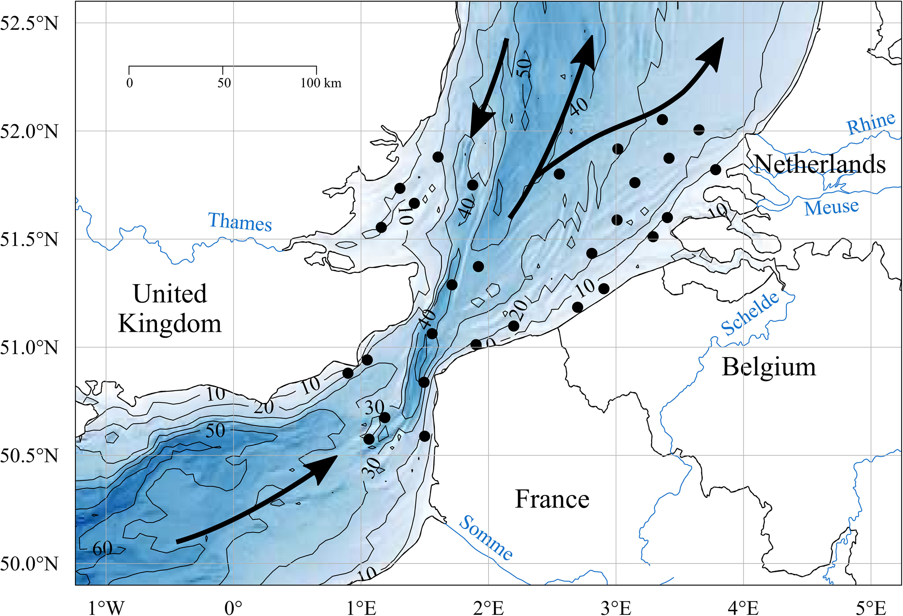
Figure 1 (IN COLOUR). Map of the study area with the black dots representing the sampling stations. The contour lines indicate the depth in meters, associated with gradual colours. The main residual currents of the study zone are indicated with the black arrows, and the main freshwater outputs by the represented rivers (blue lines).
The study area constitutes a temperate, shallow, permanently mixed system, presenting some zones of intermittent stratification such as the offshore north-eastern part of the Belgian sector and some parts of the offshore waters of the Dutch sector (De Boer et al., 2009; Van Leeuwen et al., 2015). The main freshwater inputs into the southern North Sea come from the Rhine and Meuse, and to a much lower extent from the Scheldt (Figure 1), which constitute together the main freshwater discharge of the zone, and called the Rhine-Meuse-Scheldt system throughout this article. On the coast of England and the coast of France in the English Channel, the Thames (Figure 1) and the Seine respectively constitute the main freshwater inputs (Desmit et al., 2018). For the Channel coast of France, the Somme estuary and smaller estuaries are responsible for a coastal Region of Freshwater Influence (ROFI) known as the “coastal river flow” (Brylinski et al., 1991).
As part of the H2020 JERICO-NEXT project (https://www.jerico-ri.eu/), an oceanographic campaign was carried out on board the RV “Simon Stevin” between 8th and 12th of May 2017, covering a short temporal window of the productive spring bloom season. It involved five research institutions, two from the Netherlands (RWS, NIOZ), two from Belgium (Ghent University (UGENT) and Flanders Marine Institute (VLIZ)) and one from France [Oceanology and Geosciences Laboratory (LOG)].
A total of 29 stations (Figure 1), with a minimum and maximal distance (Euclidian) of 11 and 240 km respectively from each other, were sampled for environmental parameters (defined as abiotic factors; depth, water velocity, temperature, salinity, SPM and inorganic dissolved nutrients concentrations and ratios), bacteria, protists, pigments and zooplankton. Several sampling and analytical methods for characterizing the plankton compartment were applied, resulting in the consideration of five ecosystem components in addition to the abiotic factors: bacterial diversity analysed by amplicon sequencing, protist diversity (at the genus level) analysed with the FlowCAM, pico- to micro-plankton groups abundance analysed by flow cytometry (CytoSense), pigment concentrations analysed by HPLC and zooplankton taxonomic group abundances analysed with the ZooScan. The sampling and analytical methodologies are presented for each ecosystem component separately in the following sections.
Abiotic Parameters
At every station, discrete water samples were taken at 3 meters depth by means of six Niskin bottles (5 L) attached to a CTD-carrousel (Seabird SBE25plus). For each sample, 200 mL of sea water were then filtered through a 47 mm, 0.2 µm cellulose-acetate filter (Sigma-Aldrich). The filtrates were analysed using a SEAL QuAAtro analysis for concentrations of dissolved inorganic silica, phosphorous, ammonium, nitrite, and nitrate (expressed in µmol L-1). Total nitrogen was calculated by computing the sum of ammonium, nitrite and nitrate. Full protocols are described in Mortelmans et al. (2019a). The SPM data were generated using a generic multi-sensor algorithm (Nechad et al., 2010) applied to the red remote sensing reflectance band (665 nm) available on the CMEMS server (OCEANCOLOUR_ATL _OPTICS_L3_REP_ OBSERVATIONS_009_0661). Additional parameters originating from an underway data acquisition system were selected based on the time of arrival at each station, and include depth, temperature and salinity (SBE21 sensor). Associated current velocities were obtained based on the sdmpredictors R-package using mean surface current velocities (BO2_curvelmean_ss) from bio-ORACLE v2.0 >(Tyberghein et al., 2012; Assis et al., 2018).
Amplicon Sequencing of Bacteria
A subsample of seawater from the sampler carousel (3 m depth) was filtered over a 25 mm 0.22 µm polycarbonate filter (mixed cellulose ester membrane GSWP filter, Merck) until saturation. After filtration the filter was stored in a 1.5 mL Eppendorf tube, snap frozen and transported to the laboratory in liquid nitrogen, where it was transferred for storage in the -80°C freezer until analysis. Extraction and isolation of genomic DNA included a beat-beating method with phenol-chloroform extraction based on the protocol of Zwart et al. (1998).
For each sample, bacterial amplicon libraries were constructed. For bacteria, the V1-V3 regions of the 16S SSU rRNA gene were amplified using the forward primer pA (5′-AGAGTTTGATCCTGGCTCAG-3′) (Edwards et al., 1989) and reverse primer BKL1 (5′-GTATTACCGCGGCTGCTGGCA-3′) (Cleenwerck et al., 2007). Amplifications were performed in duplicates with Polymerase Chain Reaction (PCR), using 2.5 µL PCR reaction buffer, 2.5 µL dNTP (2 mM) (Life technologies Inc.), 0.25 µL Fast Start High fidelity Taq polymerase (Roche Inc.), 2 µL of 16s and 18s SSU rRNA primer (0.25 μM) and 1 μL of extracted DNA. Sterilized HPLC grade water was added to obtain a final volume of 25 μL.
The PCR-program started with a DNA denaturation step of 96°C for 5 min, followed by 35 cycles of denaturation at 96°C for 1 min, annealing at 52-57°C for 1 min, extension at 72°C for 3 min, and a final elongation at 72°C for 20 min. The PCR products were purified with Agencourt AMPure XP beads (Beckman Coulter Inc.), duplicates were pooled after quality control with a BioAnalyzer (Agilent Inc.) and Qubit (Thermo Fisher Inc.) and the amplicon libraries were barcoded using the NEXTERA XT DNA kit (Illumina Inc.). High throughput sequencing was performed using a 300bp paired-end Illumina MiSeq machine (MiSeq, Edinburgh genomics). The forward and reverse reads were merged using Pear (Paired-End reAd merger) v.0.9.11. The UPARSE pipeline (Edgar, 2013) was used for dereplication, removal of singletons, removal of chimera’s and de‐novo clustering to the 97% similarity level and to transform the raw sequences to Operational Taxonomic Units (OTU). The Bayesian classifier of Mothur v.1.39.5 was used, with a cut-off of 80 to blast the bacteria against the SILVA Ribosomal Reference database (SILVA SSU Parc, version 123 (Yilmaz et al., 2014). Unclassified OTU’s were removed from the dataset. A threshold of 1x10⁻⁵ was used to create a binary outlier variable to remove species with low variances. The Trimmed Mean of Mu;-values (TMM) was used to calculate standardization factors to normalise the data (Robinson et al., 2010; Robinson & Oshlack, 2010) and systematic variability (false positive) was removed. The bacterial groups obtained were expressed in standardized number of reads per OTU per sample and the whole component is referred to as “Bacteria” in the rest of the present paper.
Protists via FlowCAM Analysis
The larger size fraction of the protists (>55 µm) was collected by filtering 50 L of surface water through a 55 µm Apstein net. The content of the cod end was retrieved and preserved in 2-5% final concentration acid Lugol solution and stored in dark conditions at 4°C. The samples were brought and stored at VLIZ marine station before being analysed with the FlowCAM VS-4 (Fluid Imaging Technologies), which combines the technology of flow cytometry, camera and microscopy (Álvarez et al., 2011). Before processing, the samples were sieved over a 300 µm mesh to remove large colonies (which clog the FlowCAM flow cell) and diluted when necessary. Thus, it is important to stress that the results will not comprise plankton colonies and individuals larger than 300 µm or protists smaller than 55 µm.
For each sample, 15 mL was then processed at a flow rate of 1.7 mL min-1, using a FC300 flow cell and a 4X objective. The AutoImage mode captures 20 frames per second, imaging every particle between 70 to 300 Equivalent Spherical Diameter (ESD). The Region of Interest (ROI) per frame were semi-automated identified with the auto-classification tool of VisualSpreadsheet software, using the filters based on a reference library learning set created for the Belgian Part of the North Sea (BPNS) within the LifeWatch framework (Amadei Martínez et al., 2020).
The learning set consists of 26 libraries, each with their own filter. Then, the classification was manually validated to remove the errors of the automatic prediction (using books of Tomas, 1997; Kraberg et al., 2010 and Alfred Wegener Institute for Polar and Marine Research (AWI), 2020). Finally, abundances (cells per Liter) were calculated, dividing the total number of counts per taxon by the fluid volume imaged, the volume of water filtered and the dilution factor (Amadei Martínez et al., 2020). Only plankton genera were considered in the statistical analysis since the FlowCAM also provides counts for non-organic particles such as detritus (pieces of plants, plastics, etc.), air-bubbles and camera artefacts. In addition and in relation to the scope of the initial project, only autotrophic groups have been considered in the analysis. Thus, apart from two genera not strictly autotrophic considered (Protoperidinium and Tripos, being heterotrophic and mixotrophic respectively), the nano-and micro-heterotrophic groups are not part of the data-set. This FlowCam data-set is referred to as “Protist-FlowCAM” in the rest of the manuscript.
Protists via Flow Cytometry
A CytoSense® (Cytobuoy b.v., the Netherlands) automated flow cytometer (FCM) was connected to the RV Simon Stevin underway data acquisition system, which pumps sea water at 3 m depth, for in situ protists measurements. This device is a “pulse shape-recording” flow cytometer, which records the complete scatter and fluorescence pulse shape of each particle (1-800 µm) that passes the laser beams. Particles are pumped with a calibrated peristaltic pump to pass the laser beams in a laminar flow, ensuring a single-cell/particle analysis of the samples.
The flow cytometer is equipped with two lasers, a blue (488 nm – 50 mW solid-state laser (Coherent Inc.) and a red one (635 nm – 50 mW solid-state laser (Coherent Inc.)). To capture the scattered and fluorescent light, the flow cytometer records the forward scatter signal (FWS) through a PIN photodiode and the sideward scatter (SWS), fluorescence orange (FLO) (536-601 nm), fluorescence yellow (FLY) (601-668 nm) and fluorescence red (FLR) (668 – 734 nm) on PhotoMultiplier Tubes (PMT). A measurement protocol with a pump speed of 2.1 µL s-1 was applied for six minutes, resulting in an analysed volume of on average 500 µL per sample (favouring small cells counting). The sensitivity of the PMT was set for SWS = 60, FLO = 80, FLY = 80, FLR1 (FLR 488 nm laser) = 95, FLR2 (FLR 635 nm laser) = 95. A trigger was set on the SWS (29 mV) to eliminate background noise and unwanted particles. To remove unwanted non-fluorescent particles an additional trigger was applied, respectively on maximum fluorescence red on the blue laser (FLR1 max 6).
Prior to the clustering analysis the generated dataset required pre-processing to remove signals from unwanted particles. All pre-processing was carried out with the Cytoclus 3 v3.7.4.14 software (Cytobuoy b.v., the Netherlands). Protist clusters were defined based on their light scattering and fluorescence properties using Easyclus version 1.28 (Easyclus© v1.28, Thomas Rutten Projects, the Netherlands). Two different clustering tools were combined. The first one was the lasso tool, which used a training dataset to define polygons (lasso’s) around the Synechococcus and Cryptophytes clusters, thus defining the polygons to be used to cluster the rest. The defined selection sets of the lasso tool were then combined with the size fractionation (pico <3 µm; nano 3-20 µm; micro >20 µm), based on the length measurement obtained from the FWS signal, in the fixed clustering tool. Following this approach, a total of 5 clusters were defined: pico-red, nano-red, micro-red, pico-Synecho and nano-Crypto, which correspond to standardized flow cytometer cluster names being respectively eukaryote pico-phytoplankton, eukaryote nano-phytoplankton, micro-phytoplankton, Synechococcus and Cryptophytes (www.bodc.ac.uk) (Table 1). The abundance of individual clusters was expressed in cells L-1. This component is referred to as “Protist - FCM” in the rest of the paper.
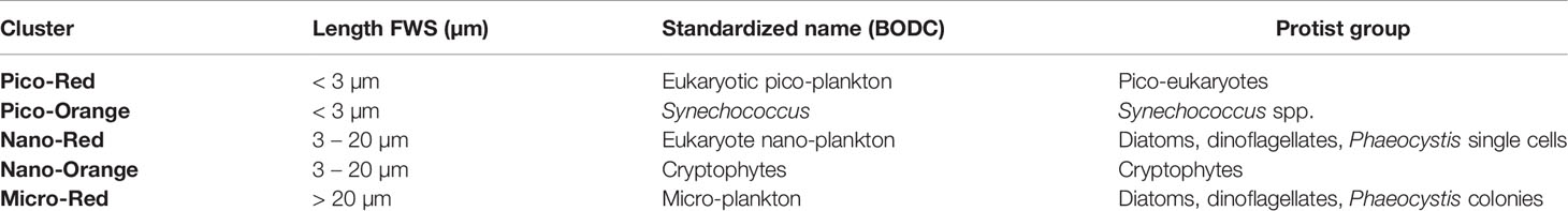
Table 1 Protist clusters detected by FCM, standardized names (https://www.bodc.ac.uk/resources/vocabularies/vocabulary_search/F02/) and main species/groups contributing to these clusters (Roy et al., 2011).
Pigments via HPLC Analysis
The water samples for the pigment analysis were obtained from the same six Niskin bottles (5 L) deployed at 3 m depth and used for the nutrient analysis. Using a vacuum pump, the water was filtered on a 47 mm, 0.4 µm glass fibre filter (Whatman GF/F) up to saturation. Immediately after filtration, the filter was stored in a 1.5 mL Eppendorf tube, snap-frozen in liquid nitrogen and kept frozen at -80°C until analysis. Pigments were extracted in 90% HPLC grade acetone and sonicated for 30 seconds at 40 Hertz. After extraction, the extracts were immediately analysed by reverse phase HPLC following the protocol described by Van Heukelem and Thomas (2001), using an Agilent 1100 series HPLC system, with an Agilent Eclipse XDB-C8 column. Marker pigments of key phytoplankton groups were identified based on their retention time and absorption spectra and were validated using pure pigment standards (DHI Denmark). The final concentrations are expressed in µg per L. and we refer to this component as “Pigment”. The different pigments analysed can be seen listed in Table Ain theSupplementary Material.
Zooplankton via ZooScan Analysis
Zooplankton was sampled at each station with a 200 µm-mesh size WP-2 net, with a flow-meter attached to the frame, and deployed vertically from near-bottom to surface. Organisms collected in the cod-end were immediately preserved on-board with 7% buffered-formaldehyde and then stored, after the campaign, at the Marine Station Ostend, Belgium (MSO). Each sample was analysed with a ZooScan and processed with the Zooprocess software for semi-automated zooplankton identification (Gorsky et al., 2010). For more details on these specific steps, see Mortelmans et al. (2019b). The learning set used consists of 22 zooplankton taxa (at the class, phylum or order level) and one detritus group. These groups have been specifically created for the BPNS within the framework of the LifeWatch program (Mortelmans et al. 2019b). Noctiluca is a heterotrophic dinoflagellate of very large size, which is not adequately quantified by the method used for the protist-FlowCAM here. Since the ZooScan better quantifies the abundances of this group, Noctiluca has been considered within the zooplankton component in this paper. The final classification was manually validated to ensure the data quality. Zooplankton counts were then expressed as abundance (individuals per L.) using the sampled volume calculated from the flow meter data.
Summary: Planktonic Compartment
The different plankton compartments considered in this study and their sampling and analysis details are summarized in Table 2.
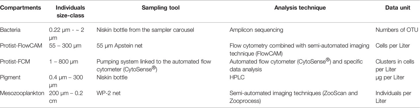
Table 2 The five biotic plankton compartments with their respective sampled size-classes, sampling tool, analysis techniques, and final data units produced.
Data Analysis
The six ecosystem components (the abiotic component and the five biotic ones) were simultaneously analysed by focusing on the structural commonalities between the six “sampling stations × variables” data tables.
While some overlap exists in terms of size range amongst some biotic components, each of them represents a different and complementary ecological information justifying the inclusion of all components in a single analysis. The data set can be viewed as six sets of variables returning six spatial distributional patterns with their respective specificities, but also with potential commonalities.
In order to simultaneously handle the spatial variability of the six ecosystem components, the STATIS method was used (Structuration des Tableaux A Trois Indices de la Statistique; Abdi et al., 2012). STATIS is a multi-table ordination technique, which goes beyond traditional multi-variable analyses such as Principal Component Analysis (PCA) since it takes into account the importance of both individual variables and data tables on the multivariate axes (Thioulouse et al., 2018). Prior to the analysis, the data were appropriately transformed. Abiotic descriptors, given their different measurement units, were standardized (centred and reduced). Ranges of biotic descriptors strongly differed between tables so that non-zero values (presences) were rescaled between 1 and 5 within tables (intervals of 0.2 quantiles), after which they were centred.
The STATIS method proceeds in two main steps. Firstly, it builds a matrix of correlations between tables using the vectorial correlation RV (Robert & Escoufier, 1976), a multivariate equivalent of Pearson’s r-correlation coefficient. This matrix is then diagonalized to generate a system of axes called the “interstructure”, enabling the ordination of tables as in PCA, showing the degree of structural similarity between ecosystem components. Secondly, the first interstructure axis score, indicating the average correlation strength of each table with the others, is used to weight tables, in order to give them more or less importance in a second system of axes, called the “compromise”. Compromise axes are built from the sum of the six station-vector correlation matrices, maximizing the overall covariation between tables and providing synthetic scores of stations as an average spatial pattern associated to the projections of ecosystem component descriptors. Hence, the compromise axes were used to represent small- to larger-scale variations of the pelagic plankton system. A given ecosystem component may not be necessarily expressed on all compromise axes, and thus, we also considered the projections of the six separate PCA axes onto the STATIS compromise axes. The analysis was carried out in R 4.0.3 (R Core Team, 2020) with the package “ade4” (Chessel et al., 2004; Dray et al., 2007).
Results
Abiotic Aspects and Total Densities of the Biotic Components
Figure 2 displays the spatial variations of the abiotic descriptors in the study area; complementarily, Table 3 provides statistical details on each descriptor. Chlorophyll a is also displayed as it is a core parameter measured in oceanographic studies. For conciseness, we will refer hereafter to “west coast” for the UK coast, and to “east coast” for the coast of continental Europe.
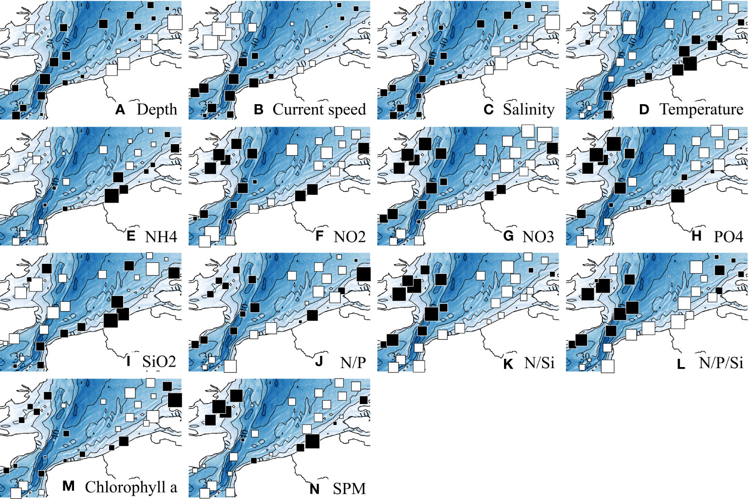
Figure 2 Spatial distributions of abiotic descriptors. Chlorophyll a is also displayed as it is a core parameter measured in oceanographic studies. Values, after ln-transformation, were standardized with mean = 0 and SD = 1. White and black squares, values respectively lower and greater than the mean; square size is proportional to the deviation from the mean. Statistical details of each descriptor are provided in Table 3.
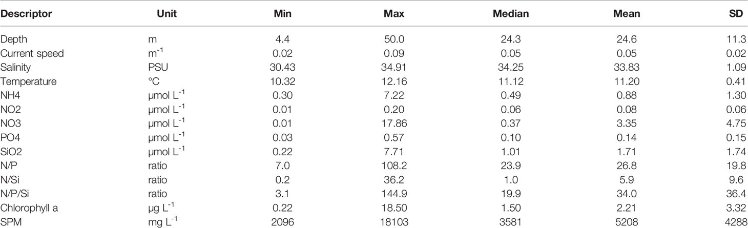
Table 3 Descriptive statistics of abiotic variables.
The depth pattern reflected the nearshore-offshore gradient. Current speeds were highest in the Strait of Dover, and tended to be overall lower in the shallower coastal zones. Salinity was lowest in the Belgian and Dutch coastal waters. Although the east coast was warmer, the thermal range of variation remained limited (10.3°C min – 12.2°C max). Nutrient concentrations and ratios were overall higher in shallow coastal waters, although high values were more homogeneously found in the western part, except for NH4 and SiO2, in higher concentrations along the eastern part. Whereas SPM concentrations decreased with depth according to a nearshore-offshore gradient, the pattern in Chlorophyll a was less clear, with lowest values isolated in the southwest and northeast zones of the study area.
Figure 3 displays the spatial variations of each biotic component total densities; complementarily, Table Ain theSupplementary Material provides statistical details for the descriptors of each biotic component. Lowest bacterial densities were concentrated around the Strait of Dover and the west side, without much variations elsewhere (Figure 3A). Protist-FlowCam densities globally decreased from the nearshore to the offshore from both west and east sides (Figure 3B), whilst Protist-FCM densities exhibited opposite trends (Figure 3C). Pigment distribution (Figure 3D) was quite similar to Chlorophyll a distribution (Figure 2M), with lowest values isolated in the southwest and northeast zones. Zooplankton density exhibited the clearest pattern with highest densities concentrated along the east coast (Figure 3E).
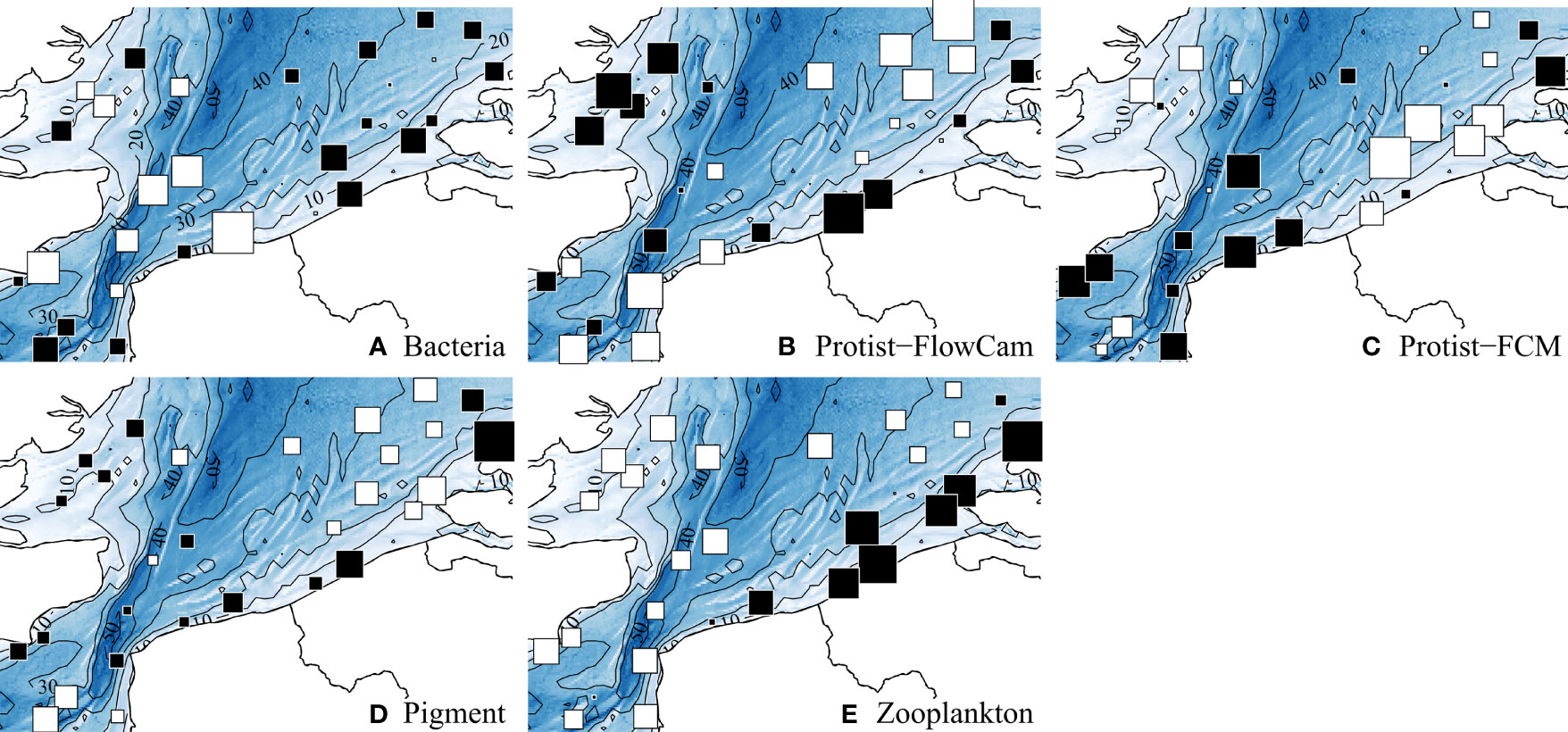
Figure 3 Spatial distributions of the total density for each biotic component. Values were standardized with mean = 0 and SD = 1. White and black squares, values respectively lower and greater than the mean; square size is proportional to the deviation from the mean. A summary of the ranges is provided in the supplementary material, Supplementary Material.
STATIS Analysis: Relationships Between Ecosystem Components (Interstructure)
The STATIS interstructure, i.e. the relationships between the ecosystem components, is displayed on Figure 4 and shows a general uni-dimensional pattern as all components were mostly correlated along the first axis. This indicated that the ecosystem components were not independent from each other and that they reflected a common spatial pattern. As displayed in Table 4, correlations between ecosystem components were relatively homogeneous (weight around 0.40 for each component) with Bacteria and Pigment showing respectively the lowest weight (0.38 and 0.39) and Protist-FlowCAM the highest (0.45).
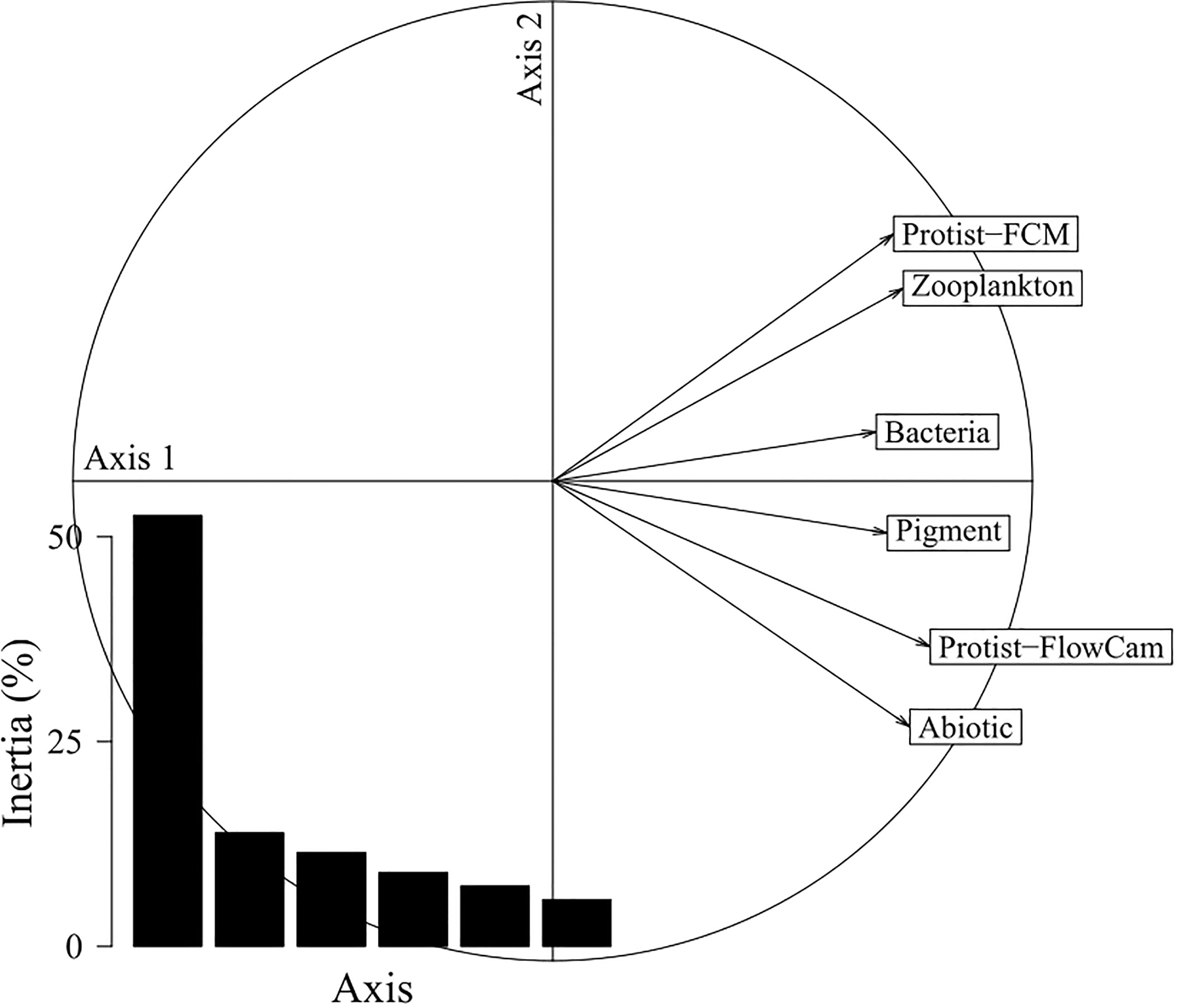
Figure 4 STATIS interstructure correlation circle. Bar diagram, eigenvalues showing the uni-dimensional nature of the pattern, with ecosystem components being mainly correlated with the dominant first axis (53%). Correlations between ecosystem components (RV-coefficients) are provided in Table 4.
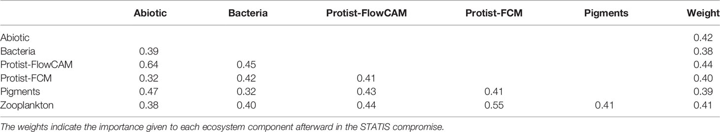
Table 4 RV correlations between ecosystem components.
STATIS Analysis: Spatial Patterns (Compromise)
Three main axes emerged from the STATIS compromise, representing nearly 50% of the total variance of the data set (Figure 5A). The scores of the sampling stations for these three axes are mapped in Figures 5B–D.
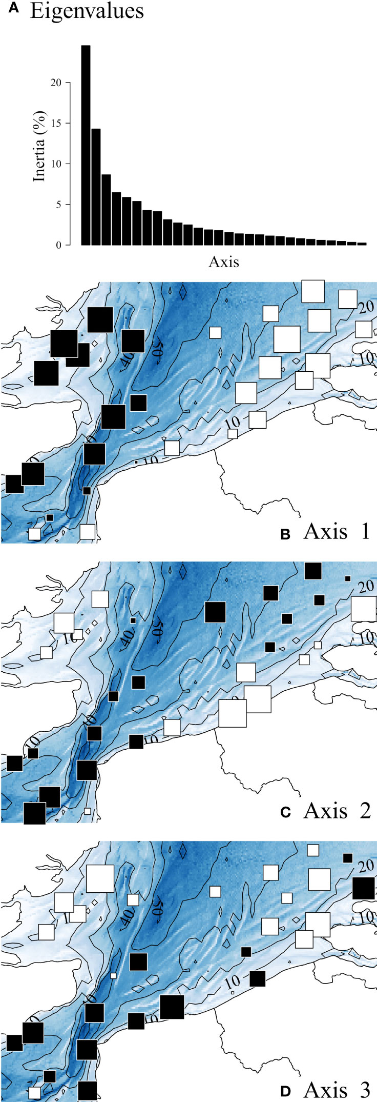
Figure 5 STATIS compromise. (A) Eigenvalue diagram showing three dominant axes: axis 1: 25%; axis 2: 14%; axis 3: 9%. (B–D) Spatial distributions of compromise axis scores. White and black squares, values lower and greater than the mean axis score (0) respectively; square size is proportional to the deviation from the mean.
This first axis of the STATIS compromise (Figure 5B), was spatially expressed as a longitudinal gradient opposing the western (coastal areas of the UK, high axis scores) to the eastern part (coastal areas of continental Europe, low axis scores) of the study area. The second axis of the STATIS compromise (Figure 5C) mainly reflected nearshore-offshore gradients with positive scores in the offshore zone. The third axis (Figure 5D), mainly opposed the southern from the northern parts.
The contributions of each ecosystem component to each compromise axis are displayed in Figure 6. All components substantially contributed to the first axis (as seen on the correlation circles). Globally, the total ecosystem component covariation with the compromise was best for Protist-FlowCAM and Abiotic descriptors, unlike Bacteria and Zooplankton for which projections were limited to the first compromise axis (RV-coefficients, Figure 6), and in agreement with their respective contribution to the initial STATIS interstructure.
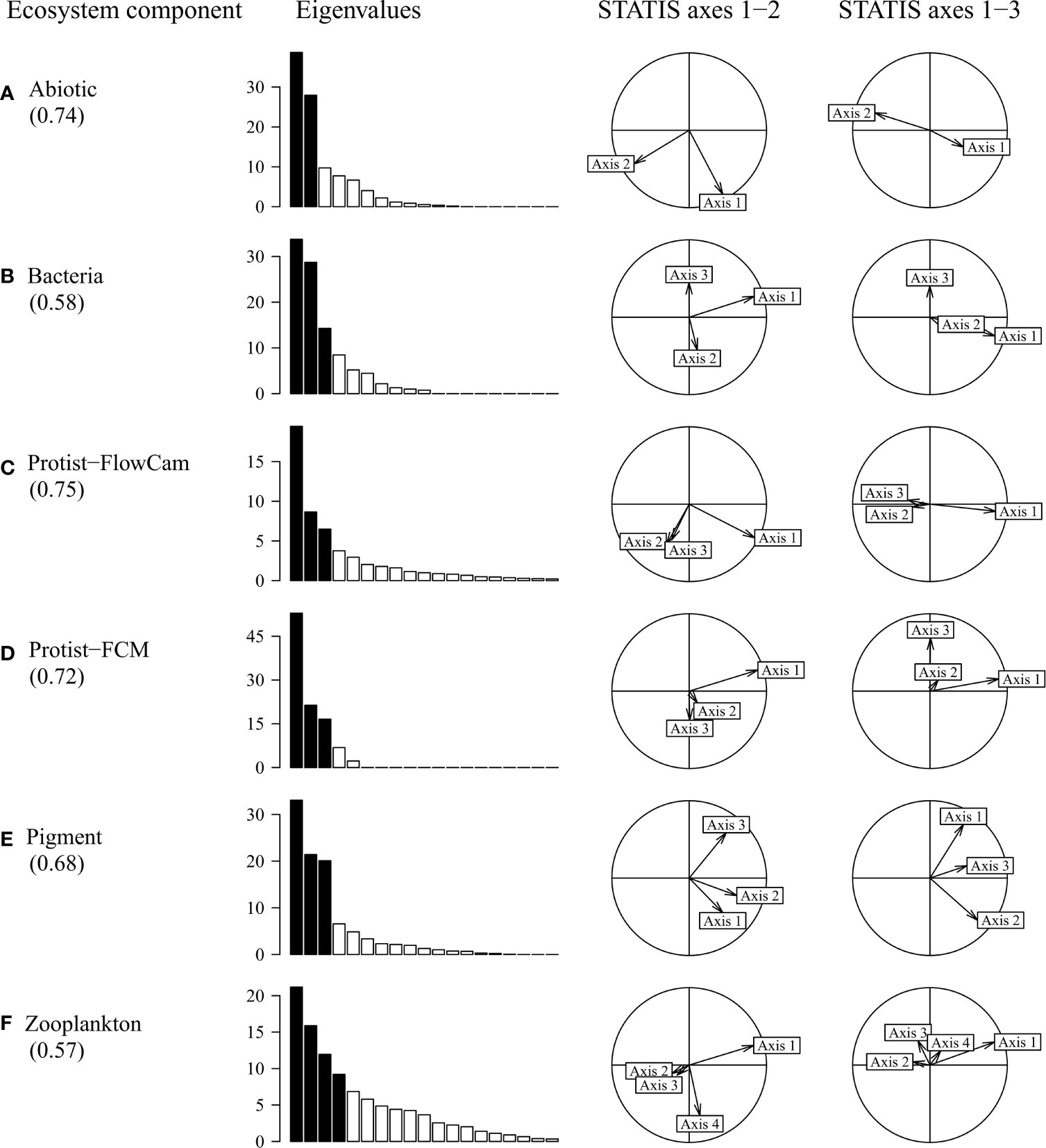
Figure 6 Ecosystem component importance on the STATIS compromise axes. Values within parentheses below each component represent the RV-coefficients indicating the covariant part of the ecosystem component with the overall compromise (fitting between separate PCA axes and compromise axes). For each ecosystem component, the eigenvalue diagram (% of total inertia) indicates the dimensionality of the PCA data structure; black bars, most contributing axes. The correlation circles display the projections of these contributing axes (vectors) onto the three STATIS compromise axes (spatial patterns from Figures 5B–D): Axis 1, horizontal; Axis 2, first column, vertical; Axis 3, second column, vertical; the degree of PCA axis projection (i.e. vector length) indicates where the interpretation of individual variables is relevant in Figures 7 and 8.
All ecosystem components contributed significantly to the first STATIS compromise axis (Figure 6). In comparison, bacteria, Protist-FCM and Zooplankton had a lower contribution to the second STATIS compromise (Figures 6B,D, F). The third axis resulted mostly from the covariation of Protist-FCM and Pigment (Figures 6D, E).
In Figure 6A, the PCA of Abiotic component returned two main axes that were mostly correlated with the two first STATIS axes (left correlation circle), whereas these two axes were weakly expressed on the third STATIS axis (right correlation circle, vertical axis). By contrast, Zooplankton (Figure 6F) shows a more complex PCA structure, expressed mostly on the first STATIS axis, the fourth Zooplankton axis (fourth eigenvalue) inducing little variance on the second STATIS axis; no Zooplankton axis was substantially expressed on the third STATIS axis.
Interplays between ecosystem component descriptors on the compromise axes are provided in Figure 7 for axes 1 and 2, and in Figure 8 for axes 2 and 3. In Supplementary Material, Table B provides correlations between descriptors and axes, and Supplementary Figures C-G and G provide the spatial distribution of each descriptor, respectively for Bacteria, Protist-FlowCAM, Protist-FCM, Pigment and Zooplankton.
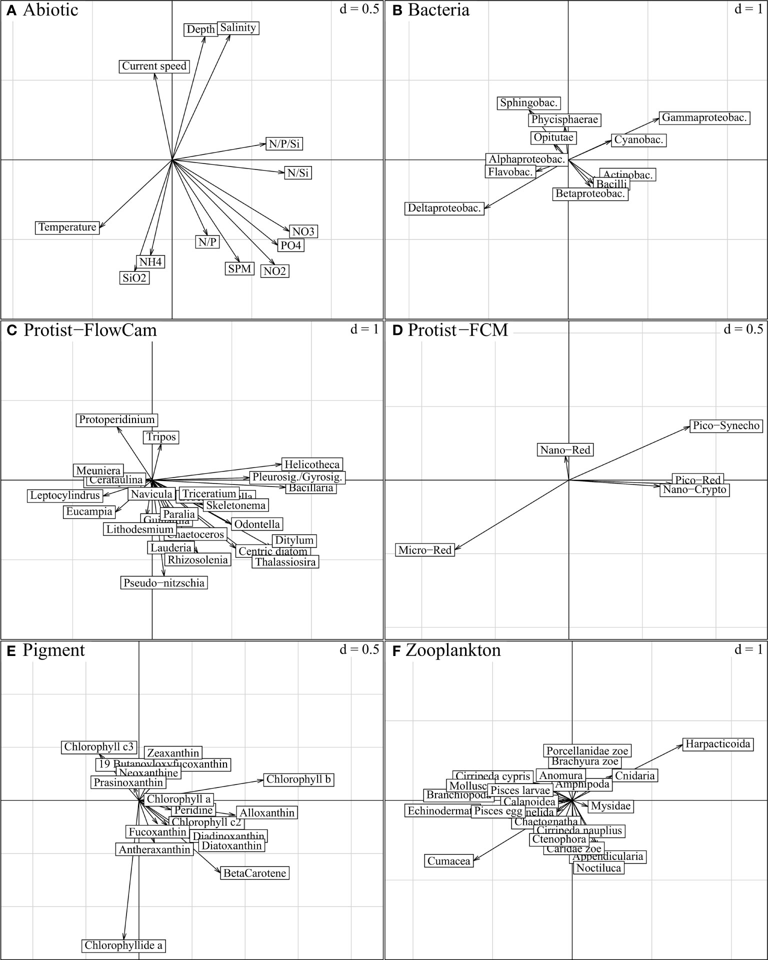
Figure 7 STATIS compromise, projection of descriptors per ecosystem component on compromise axis 1 (horizontal) and axis 2 (vertical); “d” indicates the grey grid scale, i.e. the axis unit. The variables expressed on these axes characterise the spatial variations in Figure 5B (axis 1; from left to right, east-west gradient) and Figure 5C (axis 2; down-top, nearshore-offshore gradient), respectively. Both axes are characterized by nutrient load variations, physical aspects being more specific to axis 2 (A). Biotic entities associated to these physico-chemical gradients are best represented by the longest and respectively collinear vectors in (B-F). As emphasized in Figure 6 (“STATIS axes 1-2”), most ecosystem components are expressed on both axes, except Protist-FCM with lower expression on the second axis.
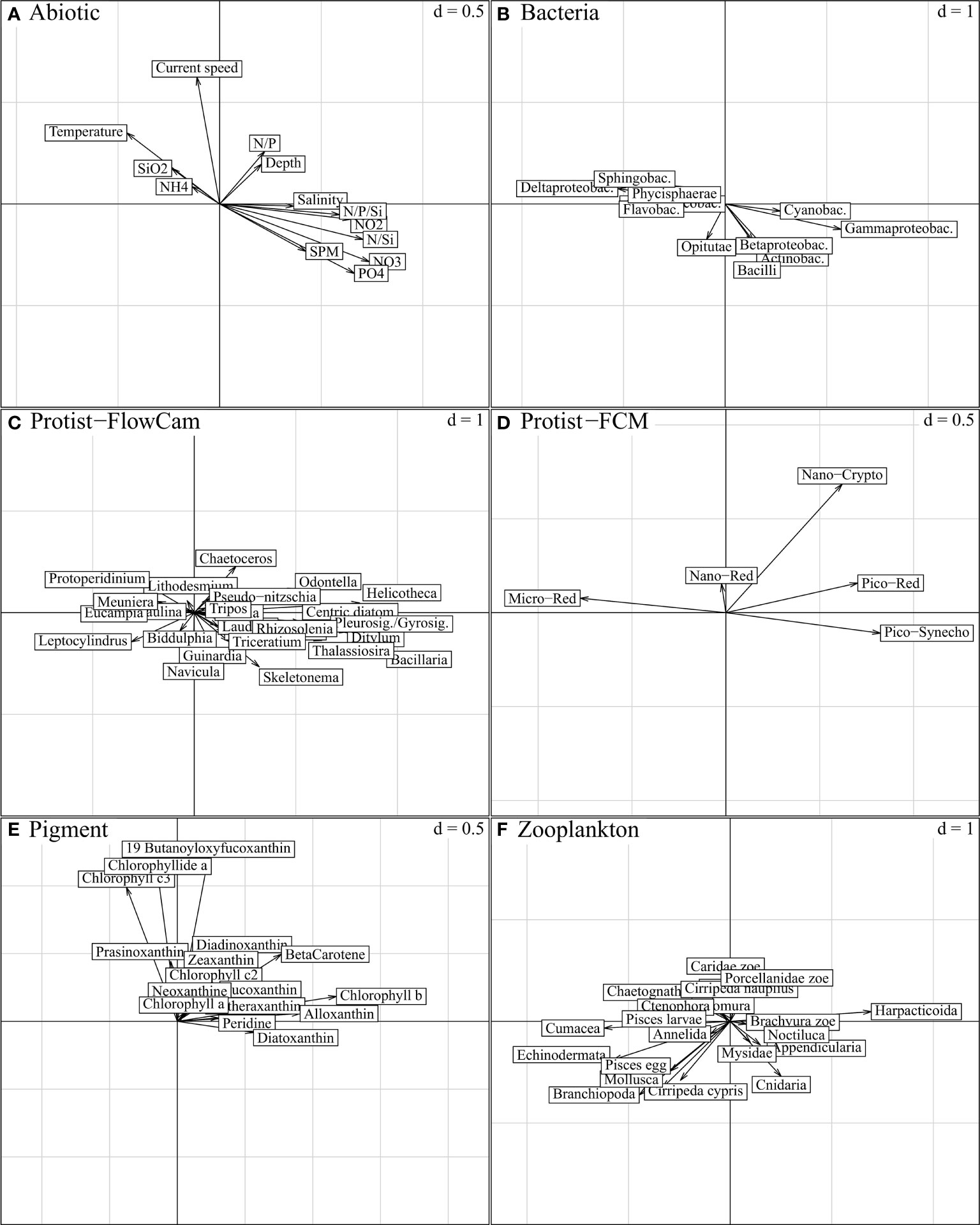
Figure 8 STATIS compromise, projection of descriptors per ecosystem component on compromise axis 1 (horizontal) and axis 3 (vertical); “d” indicates the grey grid scale, i.e. the axis unit. The variables expressed on these axes characterize the spatial variations in Figure 5B (axis 1; from left to right, east-west gradient) and Figure 5D (axis 3; down-top, north-south gradient), respectively. Axis 1 is mainly characterized by nutrient load variations, and associated biotic entities are best represented by the longest and respectively collinear vectors in (B–F). As emphasized in Figure 6 (“STATIS axes 1-3”), only Protist-FCM and Pigment components are substantially expressed on both axes. Axis 3, with limited abiotic significance, is mostly a combination of Nano-Crypto protists (D) and some pigments (E).
The first axis was strongly explained by the nutrient concentrations and ratios (NO2, NO3, PO4, N/P/Si and N/Si) (Figures 7A and 8A), consistently with the longitudinal trends visible in Figure 5B, which increased from the left to the right side of the axis (from the eastern to the western part, respectively). Among biotic components, size effects (multiple and positive covariances) were the most prominent features along this gradient. Most Protist-FlowCAM and Pigment descriptors (9 out of 16) covaried to the western part (Figures 7C, E); Bacillaria, Helicotheca and Pleurosigma/Gyrosigma were the most strongly characteristic taxa, followed by Ditylum, Odontella, Thalassiosira and other centric diatoms (Figure 7C and Supplementary Figure D); chlorophyll b, alloxanthin and beta-carotene, followed by diatoxanthin and diadoxinoxanthin were the most characteristic pigments (Figure 7E). Reversely, most Zooplankton descriptors positively covaried to the east coast, especially represented by Cumacea, Echinodermata and Branchiopoda, and with Harpaticoida more specific to the western part (Figure 7F). More symmetrically, Bacteria were represented in the western part by Gammaproteobacteria, and, to a lesser degree, Actinobacteria and Cyanobacteria; Deltaproteobacteria and Flavobacteria were the main representative of the eastern part (Figure 7B). Pico-Red, Pico-Syneco and Nano-Red were the dominant Protist-FCM clusters in the western part, opposed to Micro-Red, highly specific to the eastern part (Figure 7D). Nano-Crypto to a smaller extent was associated with the western part but only in the Strait of Dover.
The second axis, as a nearshore-offshore gradient (Figure 5C), showed increasing depth and current speed from the lower to the upper part of the axis (Figure 7A). Offshore stations (positive axis scores, Figure 5C) included those located in the Strait of Dover and accurately aligned with the main SW-NE directed inflow of Atlantic water (Figure 1). In addition, the negative axis scores were associated with high values of SiO2 and NH4+and SPM, nutrients, and less specifically high temperature, N/P ratio and nutrient contents (NO2 and PO43; Figure 7A) which corresponded to the characteristics of the stations in the coastal shallow areas (Figure 2).
Most Protist-FlowCAM taxa, especially the pennate diatom Pseudo-nitzschia (due to its high abundance in the coastal BPNS; Supplementary Figure D), and the centric diatoms Lauderia, Rhizosolenia, Thalassiosira and Lithodesmium (Figure 7C) were associated with the low axis scores and thus with the coastal areas. The dinoflagellates Protoperidinium and Tripos, heterotrophic and mixotrophic genus respectively, were the only taxa specific to the high axis scores, and thus to the offshore zone and the coastal stations in the Strait of Dover (Figure 7C). The main pigments associated with the coastal waters were chlorophyllide a, betacarotene, fucoxanthin and antheraxanthin in opposition to zeaxanthin characterizing the offshore zone (Figure 7E). The bacterial signature was limited to an offshore-nearshore opposition of Sphingobacteria and Gammaproteobacteria to Deltaproteobacteria (Figure 7B and Supplementary Figure C). Zooplankton was only expressed by its fourth axis (Figure 6), and no clear trends could be distinguished on this second axis due to the absence of dominance in the offshore zone (Supplementary Figure G).
The third compromise axis (Figure 8) was mostly limited to the expression of Protist-FCM and Pigment (Figures 6D, E; Figures 8D, E). Within these components, limited positive covariances could be observed for nano-Crypto, 19-butanoyloxyfucoxanthin, chlorophyll c3, chlorophyllide a and diadinoxanthin (Figures 8D, E and Supplementary Table B) and seemed to create a slight south-north gradient along the axis.
Discussion
The results from the STATIS analysis showed the existence of clear spatial gradients and pronounced commonalities in the spatial distribution of the different ecosystem components. We expected strong relationships between nutrients and bloom productivity in this period of the year (Reid et al., 1990; Nohe et al., 2020) to be the main driver of the plankton spatial structure, especially along a nearshore-offshore gradient, notably in relation to eutrophication on the coasts (Desmit et al., 2015; van Beusekom, 2018). While the nearshore-offshore gradient, indeed, significantly affected the planktonic system (STATIS axis 2; Figures 5A, C), regional contingencies in the study area between the two main coastal parts, the ROFI of the Thames in the western part and, the ROFI of the Scheldt-Rhine-Meuse in the eastern part, explained most of the variation of the planktonic structure (STATIS axis 1; Figures 5A, B). All descriptors, except zooplankton, were in higher concentrations in the ROFI of the Thames, potentially in relation to interactions within the plankton compartment but also lag effects related to preceding bloom-related events, at least at the time of sampling. These hypotheses will be further discussed in the next paragraphs. While the first two main axes were strongly related to both abiotic and biotic variations, the third STATIS axis reflected mainly biological variations in plankton along a latitudinal gradient.
East-West Contrasts in Plankton Community Structure in the Southern Bight
The main regional gradient opposed the two main ROFIs and was strongly determined by both abiotic and biotic components, particularly nutrient concentrations and phytoplankton descriptors (Protist-FlowCAM, and Protist-FCM), with higher concentrations in the Thames ROFI. High nutrients and SPM concentrations were not limited to the coastal part near the Thames estuary, and actually extended to the stations offshore and NW of the estuary, most likely explained by the extent of the estuarine output, which forms an extensive plume as shown by satellite data for the study period (NASA Worldview, 20202). Given that abiotic descriptors are known to be determinant during the productive bloom season in the area (Lefebvre et al., 2011; Desmit et al., 2015; Desmit et al., 2019), particularly in relation to nutrient load, a reversed spatial pattern could have been expected, i.e. with higher concentrations in the Scheldt-Rhine-Meuse ROFI. Indeed, the nutrient load of the Scheldt-Rhine-Meuse system is on average 6 and 7 times higher in terms of N and P respectively than in the Thames (Pätsch et al., 2004; Desmit et al., 2019). In addition, the NE-SW current along the UK coast, originating from the northern North Sea and influencing the Thames ROFI, has not been reported to be nutrient rich (Blauw et al., 2012).
The different nutrient concentrations and ratios measured in the two ROFIs thus rather suggest variations in the uptake by the biotic compartment, in agreement with the strong relationships between nutrients and bloom productivity at this period (Reid et al., 1990; Nohe et al., 2020) and the potential variability in bloom timing and bloom species composition (Moschonas et al., 2017; Browning et al., 2020). On the western side, total Protist-FlowCAM concentrations were higher (Supplementary Figure D), particularly in the Thames ROFI, and was characterized by a mix of highly silicified taxa (e.g. Ditylum) and less silicified ones [Rhizosolenia (Rousseau et al., 2002), Bacillaria and Helicotheca (Kapinga & Gordon, 1992; Mann, 2006)], by specific diatom markers (diatoxanthin and diadoxinoxanthin), as well as by Gammaproteobacteria, which have been shown to be often associated to diatoms (Bidle & Azam, 2001; Klindworth et al., 2014; Wemheuer et al., 2014). In contrast, the east exhibited lower concentrations in protist descriptors, and the most characteristic ones, i.e. micro-red and to a lesser extent chlorophyll c3 and nano-red, tend to be used as indicators of the presence of Phaeocystis (Astoreca et al., 2009; Bonato et al., 2015; Li et al., 2021). This translates into different timing of the bloom period between the two ROFIs, in agreement with the large spatio-temporal variability characterisation of bloom season of the Southern part of the North Sea, which extends from February to October (Dulière et al., 2019).
In the western part, the descriptors indicated an exponential diatom bloom phase, as a result of silica uptake (Billen et al., 1991; Rousseau et al., 2002) and potential adaptation to low silicate levels (mainly under 2 µM), a yearly characteristic of this zone (Weston et al., 2008). Protists within the micro- and nano- size classes, given their concentrations and size, were most likely responsible for most of the bulk primary producers’ biomass in agreement with a clear bloom situation (Weston et al., 2008; Mills & Arrigo, 2010). A decrease in SPM, better light conditions and important dissolved nitrogen amounts are factors most likely explaining that picoeukaryotes were also present in higher concentrations in this zone (pico-red and pico-Synecho, Supplementary Figure E) compared to the east side. Pico-plankton organisms have the ability to increase simultaneously with diatoms during diatom-dominated blooms (Barber & Hiscock, 2006) and their abundances largely outnumbered both the ones of the nano- and micro-phytoplankton groups (Protist-FCM data), a feature also confirmed for some stations of the same zone and period by Louchart et al. (2020). Low concentrations of their potential grazers, notably nano- and micro-dinoflagellates (Jeong et al., 2010), not measured in the present study, might have enhanced their presence, at least for the Thames ROFI since both nano- groups and pico-Synecho were in higher concentrations in the more southern UK coast. The bloom situation did not translate into the presence of mesozooplankton grazers in this west zone potentially due to the late diatom bloom timing rendering most mesozooplankton not able to meet their food requirement earlier in the season. Harpacticoid copepods were an exception, probably in relation to the ability of some species to withstand extreme conditions and undergo states of dormancy (Williams-Howze, 1997).
Late spring stage including the ending of a Phaeocystis globosa bloom would be the most straightforward explanation for nutrient depletion, with lower total Protist-FlowCAM concentrations in the east compared to the west (where only silicates were depleted) and despite continuous nutrient-rich river discharge in the Scheldt ROFI (also clearly indicated by the low salinities in this zone, cf. Figure 2). This is in agreement with the bloom onset occurring earlier than in the Thames ROFI (Gohin et al., 2019; Louchart et al., 2020), the latter having a peak generally in late May when the high SPM concentrations in this strong tidal mixing regime decrease (Blauw et al., 2018).
The Southern Bight of the North Sea, particularly along the coasts, is usually characterized by diatom blooms preceding, succeeding, or concomitant with a large bloom of Phaeocystis globosa that can represent 80% of the total bloom biomass (Breton et al., 2006; Lefebvre et al., 2011; Aardema et al., 2019). The presence of P. globosa suggested by our results (strong signature of micro-red, chlorophyll c3 and nano-red) was confirmed by the complementary study of Louchart et al. (2020) showing that the species was present in late spring 2017 all along the French coast by the Dover strait and the southern North sea. Most of the time, Phaeocytis globosa might have co-occurred with lower concentrations in diatoms compared to the west, with the exception of the coastal stations of the BPNS (Supplementary Figure E). The BPNS was the only zone in the east to be low in chlorophyll c3 (Supplementary Figure F) while high in micro-red concentrations related to a bloom of Pseudo-nitzschia (representing >70% of total Protist-FlowCAM abundance in the BPNS). This pennate diatom is characteristic of the intermediate assemblage and occurs before the summer season in this zone (Nohe et al., 2020). Correspondingly, the concentrations of mesozooplankton were particularly higher on the Belgian coast, potentially indicating grazing on this nano-colonial Pseudo-nitzschia (Harðardóttir et al., 2015; Hoffmeyer et al., 2020).
Interestingly, the higher mesozooplankton concentrations along the east coast do not only indicate that the earlier bloom situation was more adequate for the development of important contributor species of the meso-zooplankton communities compared to the west (Mackas et al., 2012; Mortelmans et al., 2021), but also indicates that mesozooplankton may benefit from grazing on P. globosa. In the most north-eastern side of the study area, the high characterisation by Cumacea (Supplementary Figure G) also corresponded to a strong characterisation of the zone by the indicators of P. globosa. This is in agreement with the results of Dauvin et al. (2008) which showed that Cumacea, a suprabenthic mesozooplankton group (feeding temporarily in the water-column), significantly increased its vertical migration into the water column during a P. globosa bloom in the eastern English Channel.
Nearshore-Offshore Contrast in Plankton Community Structure in the Southern Bight
The second spatial gradient depicted through the analysis corresponded to the expected nearshore-offshore trend. It directly supports the implication of Atlantic influence that strengthens the ecological contrasts with the coast, except for the coastal part of the Strait of Dover to some extent, where the Atlantic influence generally dominates over local coastal processes (Lee, 1980; Huthnance, 1991; Dulière et al., 2019). In addition, and as expected, the Atlantic influx of water from the English Channel was characterized by low SPM and low concentrations of nutrients (Ruddick & Lacroix, 2006; Desmit et al., 2015; Dulière et al., 2019).
Along the coast, the continental input could be clearly seen through high concentrations of autotrophic protists within the nano- and micro-size classes (Protist-FlowCAM, and to a lower extent nano-red from the FCM), represented by centric diatoms, with the exception of the bloom of the diatom Pseudo-nitzschia in the BPNS. This was also confirmed by the fucoxanthin signature (Claustre, 1994; Jeffrey & Vesk, 1997) in both the east and the west coastal part of the study area (Supplementary Figure F). Diatoms were more characteristic of the west coast, as seen previously, and within the centric diatoms, only Rhizosolenia was present in both coastal areas. Except in the BPNS, this taxon dominated the relative abundance of the Protist-FlowCam in the coastal stations, which has been shown to be typical of the late bloom stage and/or summer assemblage (Weston et al., 2008; Nohe et al., 2020). Another coastal feature was the strong characterisation by chlorophyllide a, exhibiting higher concentration at a few stations in the BPNS and in the most north-eastern part (Supplementary Figure F). While chlorophyllide a has been usually considered as a physiological marker of chlorophyllase-containing diatoms (Barrett & Jeffrey, 1971; Bidigare, 1989), a recent study (Helmann, 2019) suggested that it should be used as an indicator of senescent, physiologically compromised phytoplankton due to stress. The bloom of potentially toxin-producing Pseudo-nitzschia (Trainer et al., 2012; Xu et al., 2015) in the BPNS and the presence of Phaeocystis colonies in the north-east could have been thus causing stress for the other phytoplankton species present.
In agreement with the onshore-offshore gradient in salinity, SPM and nutrients, the offshore stations were, in contrast with the coastal part, poorly characterized by the large protist size-class (Protist-FlowCAM, Figure 3 and Supplementary Figure D). They were however highly characterized by higher concentrations of large heterotrophic/mixotrophic dinoflagellate taxa, Protoperidinium and Tripos. Dinoflagellates, in particular Protoperidinium, have been shown to be able to cope with highly turbulent systems (Hernández-Fariñas et al., 2014; Smayda et al., 2010), and can have a high grazing rate on autotrophic phytoplankton (Gribble et al., 2007; Grattepanche et al., 2011). While no important concentrations of autotrophic large cells were present in the offshore zone, dinoflagellates could have potentially taken advantage of the nano-plankton (nano-red), present in higher concentrations in most offshore stations, and of nano-Crypto and pico-plankton (both pico-red and pico-Synecho, cf. Supplementary Figure E) in the southwestern offshore part corresponding mainly to the Strait of Dover. Part of the nano-red might actually correspond to the diatoms of the nano size class found with the FlowCAM (i.e. Chaetoceros, Navicula, centric diatoms; Supplementary Figure D). In addition, cyanobacteria, indicated by zeaxanthin and matching the spatial distribution of pico-Synecho for the whole Strait of Dover, appeared as an important contributor to the offshore plankton pattern. These results corroborates with nano-and pico-size plankton being respectively an important proportion of the protist assemblage in the Atlantic offshore water and in oligotrophic waters more generally (Gibb et al., 2000; Marañón et al., 2003; Kostadinov et al., 2010; Marie et al., 2010; Masquelier et al., 2011). In spite of high nano- and pico-plankton concentrations in several offshore stations, the Protist-FCM component was not strongly expressed along this nearshore-offshore gradient (second STATIS axis, Figure 5c) due to a strong contribution of the pico-plankton groups to the east-west gradient (first axis, Figure 5b) but also to the differential spatial distribution of nano-Crypto according to a south-north opposition.
Latitudinal Contrasts in Plankton Community Structure in the Southern Bight
The south-north gradient drove a substantial part of the total spatial variation (STATIS axis 3, Figures 5a,d), with a strong characterisation of the south part by nano-Crypto which however did not match higher concentrations of its pigment marker, alloxanthin (Ansotegui et al., 2001). The nano-Crypto cluster, in this case, might has been rather composed of colonies of Synechococcus and Cyanobacteria, as supported by the distribution of their pigment marker zeaxanthin, and as they are known to be present in this zone (Supplementary Figure F; Mackey et al., 1996; Bonato et al., 2015). Some inconsistencies were also detected for the strong signature of the carotenoid 19-butanoyloxyfucoxanthin, defined as a clear marker of pelagophytes within the pico-size class (Irigoien et al., 2004; Raven, 2012), while its distribution did not exactly match the one of the pico-plankton groups. On the other hand, the characterisation by chlorophyll c3 for this south part, more particularly on the coast of France and in the north-easternmost zone, matched the one of the stress related pigment chlorophyllide a, most likely indicating the characteristic presence of Phaeocystis at this period (Astoreca et al., 2009; Bonato et al., 2015; Louchart et al., 2020; Li et al., 2021).
Conclusive Remarks and Implication for Monitoring Purposes
This study showed that the plankton spatial distribution during the productive spring period in the study area did not follow a unique pattern but was characterized by an overriding imprint of both local and regional drivers. High spatial heterogeneity in plankton distribution has been previously highlighted in this study area (Blauw et al., 2018; Aardema et al., 2019). However, while a nearshore-offshore gradient under Atlantic influence could be expected, spring bloom timing appeared to be a dominant driver of plankton community structure differing between the two main ROFI of the study area, bringing complementary insights on this spatial heterogeneity. By simultaneously considering several components of the plankton, our results also point to potential interactions within the plankton realm that are rarely assessed, especially at spatial scales beyond a unique sampling station.
However, while this study included five different plankton components, some plankton size-classes and groups are still missing from the analysis, limiting the extent of the data interpretation. For instance, we could infer the presence of Phaeocystis from proxies (micro-red, chlorophyll c3 and nano-red), but it would have been more adequate to assert its presence through microscopic counts, especially to provide quantitative data for such important protist biomass contributor. Blooms of colonial large protists such as P. globosa are often problematic for semi-automatic imaging devices (clogging effect) and thus, complementary classical techniques based on microscopy should complement the data analysis to allow a full coverage of the nano- and micro-protist size-classes. This is in general true for most plankton size-classes since the calibration settings and the volume of water sampled considered for semi-autonomous devices create some limitations (as an example, the calibration used for the flow cytometer, in this case study, favoured small organisms with the use of small sample volumes of 500 µL). For instance, taxonomic information for the nano-size classes complementing the data from the flow cytometer would have allowed us to better discuss potential inter-plankton relationships helping the interpretation of axis 3 and discrepancies between some descriptors. A full coverage of the plankton size-spectra would be also beneficial to address the challenging exercise in disentangling the complex interaction of abiotic and biotic factors driving the plankton distribution (Lima-Mendez et al., 2015; Bunse et al., 2016; Striebel et al., 2016). Nevertheless, in spite of missing groups, our results showed that usually neglected small components can have a preponderant structuring role as evidenced by the dominant weight of Protist-FlowCam in the STATIS analysis.
Despite some limitations, our joint analysis of abiotic factors and several plankton compartments enabled us to highlight interesting issues, particularly in the frame of monitoring. Chlorophyll a, often used as a proxy for phytoplankton biomass (Garmendia et al., 2013; Harvey et al., 2015), did not appear as an important factor contributing to the main spatial plankton distribution pattern during this period of intense production for instance. The use of chlorophyll a alone could have thus not enabled to highlight all the regional differences revealed by our analysis, with the exception of the expected nearshore-offshore gradient in protist biomass. While P. globosa is also generally considered detrimental for zooplankton grazers (Weisse et al., 1994; Rousseau et al., 2000; Nejstgaard et al., 2008), the present results suggests a positive interaction with higher planktonic trophic levels. As such, and more generally, our observations underscore that mere monitoring of bulk phytoplankton biomass is often insufficient and even inaccurate to inform about the plankton status. This strengthens the general requirement for a multi-faceted plankton monitoring which includes information on the plankton composition and which consider complementary techniques including the classical ones based on microscopy (Alvarez-Fernandez & Riegman, 2014; Aubert et al., 2017; McQuatters-Gollop et al., 2017).
Finally, only a snapshot of the seasonal cycle was considered here, and the question of temporal variability remains to be explored. The smallest planktonic size-classes (bacteria to nano-plankton) have different population dynamics compared to larger plankton (micro-phytoplankton and zooplankton) and are often neglected in monitoring programs, particularly in the frame of management strategies (Aubert et al., 2017). As they clearly constitute an important component of the plankton as demonstrated by our study, their integration in plankton studies could improve our understanding of ecosystem dynamics (Aubert et al., 2017; Chust et al., 2017; Lombard et al., 2019), especially in areas of high spatio-temporal variations such as the Southern Bight (Blauw et al., 2018; Ivanov et al., 2020). A more in depth understanding of the whole plankton dynamics, considering plankton inter-relationships, will definitely help to improve our predictability analysis in areas such the Southern Bight known to experience important bloom dynamics shifts (Aardema et al., 2019; Nohe et al., 2020; Mortelmans et al., 2021).
Data Availability Statement
The datasets presented in this study can be found in online repositories. The names of the repositories and accession numbers can be found below: https://www.ebi.ac.uk/ena/browser/view/PRJEB52461?swho=reads; Flanders Marine Institute (VLIZ): Belgium; Royal Netherlands Institute for Sea Research (NIOZ); Rijkswaterstaat (RWS): Netherlands; The National Center for Scientific Research (CNRS): France; (2022): Plankton biodiversity data from a LifeWatch/Jerico North Sea Cruise with R/V Simon Stevin in May 2017. Marine Data Archive. https://doi.org/10.14284/549.
Author Contributions
AA: validation, formal analysis, data curation, writing - original draft, writing - review and editing, visualization, supervision. OB: conceptualization, methodology, software, formal analysis, writing - original statistical methodology and results parts draft, writing - review and editing, visualization. RB: investigation, data curation, writing - original method part draft, writing - review and editing. LA: validation, writing - review and editing. KS: writing - review and editing. WV: writing - review and editing. LA: investigation, data curation, writing - review and editing. KD: conceptualization, resources, supervision, project administration, funding acquisition. AL: investigation, writing - review and editing. JM: investigation, resources, data curation, writing - review and editing. MR: investigation, data curation, writing - review and editing. ED: conceptualization, data curation, writing - original method part draft, project administration, supervision, writing - review and editing. All authors contributed to the article and approved the submitted version.
Funding
The oceanographic campaign was organised within the H2020 INFRAIA Joint European Research Infrastructure for Coastal Observatories-New Expertise (JERICO-NEXT) project (2015-2019), grant agreement N° 654410. Funding for the data collection and management were provided by VLIZ as part of the Flemish contribution to LifeWatch ESFRI.
Conflict of Interest
The authors declare that the research was conducted in the absence of any commercial or financial relationships that could be construed as a potential conflict of interest.
Publisher’s Note
All claims expressed in this article are solely those of the authors and do not necessarily represent those of their affiliated organizations, or those of the publisher, the editors and the reviewers. Any product that may be evaluated in this article, or claim that may be made by its manufacturer, is not guaranteed or endorsed by the publisher.
Acknowledgments
Dimitry Van der Zande (RBINS, Belgium) is acknowledged for providing and processing the SPM data within the DCS4COP project (European Union’s Horizon 2020 research and innovation programme, grant agreement No 776342). Finally, special thanks to Tyberghein L., Goossens J. and the crew of the RV Simon Stevin for logistical and practical support.
Supplementary Material
The Supplementary Material for this article can be found online at: https://www.frontiersin.org/articles/10.3389/fmars.2022.863996/full#supplementary-material
Footnotes
- ^ https://resources.marine.copernicus.eu/product-detail/OCEANCOLOUR_ATL_OPTICS_L3_REP_OBSERVATIONS_009_066/DATA-ACCESS
- ^ https://worldview.earthdata.nasa.gov/
References
Aardema H. M., Rijkeboer M., Lefebvre A., Veen A., Kromkamp J. C. (2019). High-Resolution Underway Measurements of Phytoplankton Photosynthesis and Abundance as an Innovative Addition to Water Quality Monitoring Programs. Ocean Sci. 15 (5), 1267–1285. doi: 10.5194/os-15-1267-2019
Abdi H., Williams L. J., Valentin D., Bennani-Dosse M. (2012). STATIS and DISTATIS: Optimum Multitable Principal Component Analysis and Three Way Metric Multidimensional Scaling. in Wiley Interdisciplinary Reviews: Computational Statistics. 6, 124–167. doi: 10.1002/wics.198
Alfred Wegener Institute for Polar and Marine Research (AWI) Plankton net. Available at: http://planktonnet.awi.de (Accessed October 2020).
Alvarez-Fernandez S., Riegman R. (2014). Chlorophyll in North Sea Coastal and Offshore Waters Does Not Reflect Long-Term Trends of Phytoplankton Biomass. J. Sea Res. 91, 35–44. doi: 10.1016/j.seares.2014.04.005
Álvarez E., López-Urrutia Á., Nogueira E., Fraga S. (2011). How to Effectively Sample the Plankton Size Spectrum? A Case Study Using FlowCAM. J. Plankton Res. 33 (7), 1119–1133. doi: 10.1093/plankt/fbr012
Amadei Martínez L., Mortelmans J., Dillen N., Debusschere E., Deneudt K. (2020). LifeWatch Observatory Data: Phytoplankton Observations in the Belgian Part of the North Sea. Biodivers. Data J. 8, e57236. doi: 10.3897/BDJ.8.e57236
Ansotegui A., Trigueros J. M., Orive E. (2001). The Use of Pigment Signatures to Assess Phytoplankton Assemblage Structure in Estuarine Waters. Estuarine Coast. Shelf Sci. 52 (6), 689–703. doi: 10.1006/ecss.2001.0785
Assis J., Tyberghein L., Bosh S., Verbruggen H., Serrão E. A., De Clerck O. (2018). Bio-ORACLE V2.0: Extending Marine Data Layers for Bioclimatic Modelling. Global Ecol. Biogeogr. 27 (3), 277–284. doi: 10.1111/geb.12693
Astoreca R., Rousseau V., Ruddick K., Knechciak C., Van Mol B., Parent J. Y., et al. (2009). Development and Application of an Algorithm for Detecting Phaeocystis Globosa Blooms in the Case 2 Southern North Sea Waters. J. plankton Res. 31 (3), 287–300. doi: 10.1093%2Fplankt%2Ffbn116
Aubert A., Rombouts I., Artigas F., Budria A., Ostle C., Padegimas B., et al. (2017). “Combining Methods and Data for a More Holistic Assessment of the Plankton Community,” in Contribution to the EU Co-Financed EcApRHA Project (Applying an Ecosystem Approach to (Sub) Regional Habitat Assessments) (London: OSPAR) 41. Available at: https://www.ospar.org/work-areas/bdc/ecaprha/reports.
Barber R. T., Hiscock M. R. (2006). A Rising Tide Lifts All Phytoplankton: Growth Response of Other Phytoplankton Taxa in Diatom-Dominated Blooms. Global Biogeochem. Cycles 20 (4), 1–12. doi: 10.1029/2006GB002726
Barrett J., Jeffrey S. W. (1971). A Note on the Occurrence of Chlorophyllase in Marine Algae. J. Exp. Mar. Biol. Ecol. 7 (3), 255–262. doi: 10.1016/0022-0981(71)90008-6
Beaugrand G., Edwards M., Legendre L. (2010). Marine Biodiversity, Ecosystem Functioning, and Carbon Cycles. Proc. Natl. Acad. Sci. United States America 107 (22), 10120–10124. doi: 10.1073/pnas.0913855107
Beaugrand G., Ibanez F. (2004). Monitoring Marine Plankton Ecosystems. II: Long-Term Changes in North Sea Calanoid Copepods in Relation to Hydro-Climatic Variability. Mar. Ecol. Prog. Ser. 284, 35–47. doi: 10.3354/meps284035
Berge T., Chakraborty S., Hansen P., Andersen K. (2017). Modeling Succession of Key Resource-Harvesting Traits of Mixotrophic Plankton. ISME J. 11, (212–223). doi: 10.1038/ismej.2016.92
Bidigare R. R. (1989). “Photosynthetic Pigment Composition of the Brown Tide Alga: Unique Chlorophyll and Carotenoid Derivatives,” in Novel Phytoplankton Blooms. Coastal and Estuarine Studies (Formerly Lecture Notes on Coastal and Estuarine Studies), vol. 35) . Eds. Cosper E. M., Bricelj V. M., Carpenter E. J. (Berlin: Springer), 57–75. doi: 10.1007/978-3-642-75280-3_4
Bidle K. D., Azam F. (2001). Bacterial Control of Silicon Regeneration From Diatom Detritus: Significance of Bacterial Ectohydrolases and Species Identity. Limnol. Oceanogr. 46 (7), 1606–1623. doi: 10.4319/lo.2001.46.7.1606
Billen G., Lancelot C., Meybeck M. (1991). “N, P and Si Retention Along the Aquatic Continuum From Land to Ocean,” in Ocean Margin Processes in Global Change, Dalhem Workshop Report. Eds. Mantoura R. F. C., Martin J. M., Wollast R. (New York: WileyLiss Inc), 19–44.
Blauw A. N., Beninca E., Laane R. W., Greenwood N., Huisman J. (2012). Dancing With the Tides: Fluctuations of Coastal Phytoplankton Orchestrated by Different Oscillatory Modes of the Tidal Cycle. PloS One 7 (11), e49319. doi: 10.1371/journal.pone.0049319
Blauw A. N., Benincà E., Laane R. W., Greenwood N., Huisman J. (2018). Predictability and Environmental Drivers of Chlorophyll Fluctuations Vary Across Different Time Scales and Regions of the North Sea. Prog. Oceanogr. 161, 1–18. doi: 10.1016/j.pocean.2018.01.005
Bonato S., Christaki U., Lefebvre A., Lizon F., Thyssen M., Artigas L. F. (2015). High Spatial Variability of Phytoplankton Assessed by Flow Cytometry, in a Dynamic Productive Coastal Area, in Spring: The Eastern English Channel. Estuarine Coast. Shelf Sci. 154, 214–223. doi: 10.1016/j.ecss.2014.12.037
Boyce D. G., Frank K. T., Leggett W. C. (2015). From Mice to Elephants: Overturning the ‘One Size Fits All’ Paradigm in Marine Plankton Food Chains. Ecol. Lett. 18 (6), 504–515. doi: 10.1111/ele.12434
Breton E., Rousseau V., Parent J. Y., Ozer J., Lancelot C. (2006). Hydroclimatic Modulation of Diatom/Phaeocystis Blooms in Nutrient-Enriched Belgian Coastal Waters (North Sea). Limnol. Oceanogr. 51 (3), 1401–1409. doi: 10.4319/lo.2006.51.3.1401
Brion N., Jans S., Chou L., Rousseau V. (2008). “Nutrient Loads to the Belgian Coastal Zone,” in Current Status of Eutrophication in the Belgian Coastal Zone. Eds. Rousseau V., Lancelot C., Cox D. (Brussels: Presses Universitaires de Bruxelles), 17–44.
Browning T. J., Al-Hashem A. A., Hopwood M. J., Engel A., Wakefield E. D., Achterberg E. P. (2020). Nutrient Regulation of Late Spring Phytoplankton Blooms in the Midlatitude North Atlantic. Limnol. Oceanogr. 65 (6), 1136–1148. doi: 10.1002/lno.11376
Brylinski J. M., Lagadeuc Y., Gentilhomme V., Dupont J. P., Lafite R., Dupeuble P. A., et al. (1991). Le Fleuve Côtier: Un Phénomène Hydrologique Important En Manche Orientale. Exemple Du Pas-De-Calais. Oceanologica Acta Volume Special 11), 197–203.
Bunse C., Bertos-Fortis M., Sassenhagen I., Sildever S., Sjöqvist C., Godhe A., et al. (2016). Spatio-Temporal Interdependence of Bacteria and Phytoplankton During a Baltic Sea Spring Bloom. Front. Microbiol. 7 (517). doi: 10.3389/fmicb.2016.00517
Capuzzo E., Lynam C. P., Barry J., Stephens D., Forster R. M., Greenwood N., et al. (2017). Decline in Primary Production in the North Sea Over 25 Years, Associated With Reductions in Zooplankton Abundance and Fish Stock Recruitment. Global Change Biol. 24 (1), e352–e364. doi: 10.1111/gcb.13916
Chain F. J., Brown E. A., MacIsaac H. J., Cristescu M. E. (2016). Metabarcoding Reveals Strong Spatial Structure and Temporal Turnover of Zooplankton Communities Among Marine and Freshwater Ports. Diversity Dis. 22 (5), 493–504. doi: 10.1111/ddi.12427
Chessel D., Dufour A. B., Thioulouse J. (2004). The Ade4 Package-I – One-Table Methods. R News 4 (1), 5–10.
Chust G., Vogt M., Benedetti F., Nakov T., Villéger S., Aubert A., et al. (2017). Mare Incognitum: A Glimpse Into Future Plankton Diversity and Ecology Research. Front. Mar. Sci. 4. doi: 10.3389/fmars.2017.00068
Cirri E., Pohnert G. (2019). Algae– Bacteria Interactions That Balance the Planktonic Microbiome. New Phytol. 223 (1), 100–106. doi: 10.1111/nph.15765
Claustre H. (1994). The Trophic Status of Various Oceanic Provinces as Revealed by Phytoplankton Pigment Signatures. Limnol. Oceanogr. 39 (5), 1206–1210. doi: 10.4319/lo.1994.39.5.1206
Cleenwerck I., Camu N., Engelbeen K., De Winter T., Vandemeulebroecke K., De Vos P., et al. (2007). Acetobacter Ghanensis Sp. Nov., a Novel Acetic Acid Bacterium Isolated From Traditional Heap Fermentations of Ghanaian Cocoa Beans. Int. J. syst. evol. Microbiol. 57 (7), 1647–1652. doi: 10.1099/ijs.0.64840-0
D'Alelio D., Eveillard D., Coles V. J., Caputi L., d’Alcalà M. R., Ludicone D. (2019). Modelling the Complexity of Plankton Communities Exploiting Omics Potential: From Present Challenges to an Integrative Pipeline. Curr. Opin. Syst. Biol. 13, 68–74. doi: 10.1016/j.coisb.2018.10.003
Dauvin J. C., Desroy N., Denis L., Ruellet T. (2008). Does the Phaeocystis Bloom Affect the Diel Migration of the Suprabenthos Community? Mar. pollut. Bull. 56 (1), 77–87. doi: 10.1016/j.marpolbul.2007.09.041
De Boer G. J., Pietrzak J. D., Winterwerp J. C. (2009). SST Observations of Upwelling Induced by Tidal Straining in the Rhine ROFI. Cont. Shelf Res. 29 (1), 263–277. doi: 10.1016/J
Desmit X., Nohe A., Borges A. V., Prins T., De Cauwer K., Lagring R., et al. (2019). Changes in Chlorophyll Concentration and Phenology in the North Sea in Relation to De-Eutrophication and Sea Surface Warming. Limnol. Oceanogr. 65 (4), 828–847. doi: 10.1002/lno.11351
Desmit X., Ruddick K., Lacroix G. (2015). Salinity Predicts the Distribution of Chlorophyll a Spring Peak in the Southern North Sea Continental Waters. J. Sea Res. 103, 59–74. doi: 10.1016/j.seares.2015.02.007
Desmit X., Thieu V., Billen G., Campuzano F., Dulière V., Garnier J., et al. (2018). Reducing Marine Eutrophication may Require a Paradigmatic Change. Sci. Total Environ. 635, 1444–1466. doi: 10.1016/j.scitotenv.2018.04.181
De Vargas C., Audic S., Henry N., Decelle J., Mahé F., Logares R., et al. (2015). Eukaryotic Plankton Diversity in the Sunlit Ocean. Science 348 (6237), 1261605–1-1261605-11. doi: 10.1126/science.1261605
Dray S., Dufour A. B., Chessel D. (2007). The Ade4 Package – II: Two-Table and K-Table Methods. R News 7 (2), 47–52.
Dulière V., Gypens N., Lancelot C., Luyten P., Lacroix G. (2019). Origin of Nitrogen in the English Channel and Southern Bight of the North Sea Ecosystems. Hydrobiologia 845 (5917), 13–33. doi: 10.1007/s10750-017-3419-5
Edgar R. C. (2013). UPARSE: Highly Accurate OTU Sequences From Microbial Amplicon Reads. Nat. Methods 10 (10), 996–998. doi: 10.1038/nmeth.2604
Edwards U., Rogall T., Blöcker H., Emde M., Böttger E. C. (1989). Isolation and Direct Complete Nucleotide Determination of Entire Genes. Characterization of a Gene Coding for 16S Ribosomal RNA. Nucleic Acids Res. 17 (19), 7843–7853. doi: 10.1093%2Fnar%2F17.19.7843
Falkowski P. (2012). Ocean Science: The Power of Plankton. Nature 483 (7387), S17–S20. doi: 10.1038/483S17a
Garmendia M., Borja Á., Franco J., Revilla M. (2013). Phytoplankton Composition Indicators for the Assessment of Eutrophication in Marine Waters: Present State and Challenges Within the European Directives. Mar. pollut. Bull. 66 (1-2), 7–16. doi: 10.1016/j.marpolbul.2012.10.005
Gibb S. W., Barlow R. G., Cummings D. G., Rees N. W., Trees C. C., Holligan P., et al. (2000). Surface Phytoplankton Pigment Distribution in the Atlantic Ocean: An Assessment of Basin Scale Variability Between 50°N and 50°S. Prog. Oceanogr. 45 (3-4), 339–368. doi: 10.1016/S0079-6611(00)00007-0
Gohin F., van der Zande D., Tilstone G., Eleveld M. A., Lefebvre A., Andrieux-Loyer F., et al. (2019). Twenty Years of Satellite and in Situ Observations of Surface Chlorophyll-a From the Northern Bay of Biscay to the Eastern English Channel. Is the Water Quality Improving? Remote Sens. Environ. 233, (111343). doi: 10.1016/j.rse.2019.111343
Gorsky G., Ohman M. D., Picheral M., Gasparini S., Stemmann L., Romagnan J.-B., et al. (2010). Digital Zooplankton Image Analysis Using The ZooScan Integrated System. J. Plankton Res. 32 (3), 285–303. doi: 10.1093/plankt/fbp124
Grattepanche J. D., Breton E., Brylinski J. M., Lecuyer E., Christaki U. (2011). Succession of Primary Producers and Micrograzers in a Coastal Ecosystem Dominated by Phaeocystis Globosa Blooms. J. Plankton Res. 33 (1), 37–50. doi: 10.1093/plankt/fbq097
Gribble K. E., Nolan G., Anderson D. M. (2007). Biodiversity, Biogeography and Potential Trophic Impact of Protoperidinium Spp. (Dinophyceae) Off the Southwestern Coast of Ireland. J. Plankton Res. 29 (11), 931–947. doi: 10.1093/plankt/fbm070
Harðardóttir S., Pančić M., Tammilehto A., Krock B., Møller E. F., Nielsen T. G., et al. (2015). Dangerous Relations in the Arctic Marine Food Web: Interactions Between Toxin Producing Pseudo-Nitzschia Diatoms and Calanus Copepodites. Mar. Drugs 13 (6), 3809–3835. doi: 10.3390/md13063809
Harvey E. T., Kratzer S., Philipson P. (2015). Satellite-Based Water Quality Monitoring for Improved Spatial and Temporal Retrieval of Chlorophyll-a in Coastal Waters. Remote Sens. Environ. 158, 417–430. doi: 10.1016/j.rse.2014.11.017
Hays G. C., Richardson A. J., Robinson C. (2005). Climate Change and Marine Plankton. Trends Ecol. Evol. 20 (6), 337–344. doi: 10.1016/j.tree.2005.03.004
Hébert M. P., Beisner B. E., Maranger R. (2017). Linking Zooplankton Communities to Ecosystem Functioning: Toward an Effect-Trait Framework. J. Plankton Res. 39 (1), 3–12. doi: 10.1093/plankt/fbw068
Helmann S. C. (2019). Chlorophyllide a: Fact or Artifact-Resolution of the Chlorophyllide a Problem in the Routine Measurement of Planktonic Chlorophyll a. Capstone Projects Master's Theses, 652.
Hernández-Fariñas T., Soudant D., Barillé L., Belin C., Lefebvre A., Bacher C. (2014). Temporal Changes in the Phytoplankton Community Along the French Coast of the Eastern English Channel and the Southern Bight of the North Sea. ICES J. Mar. Sci. 71 (4), 821–833. doi: 10.1093/icesjms/fst192
Hoffmeyer M. S., Dutto M. S., Berasategui A. A., Garcia M. D., Pettigrosso R. E., Almandoz G. O., et al. (2020). DOMOIC Acid, Pseudo-Nitzschia Spp and Potential Vectors at the Base of the Pelagic Food Web Over the Northern Patagonian Coast, Southwestern Atlantic. J. Mar. Syst. 212, (103448). doi: 10.1016/j.jmarsys.2020.103448
Huthnance J. M. (1991). Physical Oceanography of the North Sea. Ocean shoreline Manage. 16 (3-4), 199–231. doi: 10.1016/0951-8312(91)90005-M
Ibarbalz F. M., Henry N., Brandão M. C., Martini S., Busseni G., Byrne, et al. (2019). Global Trends in Marine Plankton Diversity Across Kingdoms of Life. Cell 179 (5), 1084–1097. doi: 10.1016/j.cell.2019.10.008
Irigoien X., Meyer B., Harris R., Harbour D. (2004). Using HPLC Pigment Analysis to Investigate Phytoplankton Taxonomy: The Importance of Knowing Your Species. Helgoland Mar. Res. 58 (2), 77–82. doi: 10.1007/s10152-004-0171-9
Ivanov E., Capet A., Barth A., Delhez E. J., Soetaert K., Grégoire M. (2020). Hydrodynamic Variability in the Southern Bight of the North Sea in Response to Typical Atmospheric and Tidal Regimes. Benefit of Using a High Resolution Model. Ocean Model. 154, (101682). doi: 10.1016/j.ocemod.2020.101682
Jeffrey S. W., Vesk M. (1997). “Introduction to Marine Phytoplankton and Their Pigment Signatures,” in Phytoplankton Pigments in Oceanography. Eds. Jeffrey S. W., Mantoura R. F. C., Wright S. W. (Paris: UNESCO), 37–84.
Jeong H. J., Du Yoo Y., Kim J. S., Seong K. A., Kang N. S., Kim T. H. (2010). Growth, Feeding and Ecological Roles of the Mixotrophic and Heterotrophic Dinoflagellates in Marine Planktonic Food Webs. Ocean Sci. J. 45 (2), 65–91. doi: 10.1007/s12601-010-0007-2
Kapinga M. R., Gordon R. (1992). Cell Attachment in the Motile Colonial Diatom Bacillaria Paxillifer. Diatom Res. 7 (2), 215–220. doi: 10.1080/0269249X.1992.9705214
Keeling P. J., Burki F., Wilcox H. M., Allam B., Allen E. E., Amaral-Zettler L. A., et al. (2014). The Marine Microbial Eukaryote Transcriptome Sequencing Project (MMETSP): Illuminating the Functional Diversity of Eukaryotic Life in the Oceans Through Transcriptome Sequencing. PloS Biol. 12 (6), e1001889. doi: 10.1371/journal.pbio.1001889
Klindworth A., Mann A. J., Huang S., Wichels A., Quast C., Waldmann J., et al. (2014). Diversity and Activity of Marine Bacterioplankton During a Diatom Bloom in the North Sea Assessed by Total RNA and Pyrotag Sequencing. Mar. Genomics 18 B, 185–192. doi: 10.1016/j.margen.2014.08.007
Kostadinov T. S., Siegel D. A., Maritorena S. (2010). Global Variability of Phytoplankton Functional Types From Space: Assessment via the Particle Size Distribution. Biogeosciences 7 (10), 3239–3257. doi: 10.5194/bg-7-3239-2010
Kraberg A., Baumann M., Dürselen C. D. (2010). Coastal Phytoplankton: Photo Guide for Northern European Seas. Ed. Pfeil V. Dr. F.. (München: Dr. Friedrich Pfeil), 204.
Lacroix G., Ruddick K., Ozer J., Lancelot C. (2004). Modelling the Impact of the Scheldt and Rhine/Meuse Plumes on the Salinity Distribution in Belgian Waters (Southern North Sea). J. Sea Res. 52 (3), 149–163. doi: 10.1016/j.seares.2004.01.003
Lassalle G., Lobry J., Le Loc’H F., Bustamante P., Certain G., Delmas D., et al. (2011). Lower Trophic Levels and Detrital Biomass Control the Bay of Biscay Continental Shelf Food Web: Implications for Ecosystem Management. Prog. Oceanogr. 91 (4), 561–575. doi: 10.1016/j.pocean.2011.09.002
Lee A. J. (1980). “North Sea: Physical Oceanography,” in The North-West European Shelf Seas: The Sea Bed and the Sea in Motion, II, ed. Eds. Banner F. T., Collins M. B., Massie K. S. (Amsterdam: Elsevier), 467–493.
Lefebvre A., Guiselin N., Barbet F., Artigas F. L. (2011). Long-Term Hydrological and Phytoplankton Monitorin–2007) of Three Potentially Eutrophic Systems in the Eastern English Channel and the Southern Bight of the North Sea. ICES J. Mar. Sci. 68 (10), 2029–2043. doi: 10.1093/icesjms/fsr149
Lima-Mendez G., Faust K., Henry N., Decelle J., Colin S., Carcillo F. (2015). Determinants of Community Structure in the Global Plankton Interactome. Science 348, (6237). doi: 10.1126/science.1262073
Li X., Shang S., Lee Z., Lin G., Zhang Y., Wu J., et al. (2021). Detection and Biomass Estimation of Phaeocystis Globosa Blooms Off Southern China From UAV-Based Hyperspectral Measurements. IEEE Trans. Geosci. Remote Sens. 99), 1–13. doi: 10.1109/TGRS.2021.3051466
Lombard F., Boss E., Waite A. M., Vogt M., Uitz J., Stemmann L., et al. (2019). Globally Consistent Quantitative Observations of Planktonic Ecosystems. Front. Mar. Sci. 6. doi: 10.3389/fmars.2019.00196
Louchart A., DeBlok R., Debuschere E., Gomez F., Lefebvre A., Lizon F., et al. (2020). “Automated Techniques to Follow the Spatial Distribution of Phaeocystis Globosa and Diatoms Spring Blooms in the Channel and North Sea,” in Proceedings of the ICHA2018 (18th International Conference on Harmful algae, Nantes 21-26 October 2018). Nantes: International Society for the Study of Harmful Algae (ISSHA), Institut Francais de Recherche pour l'Exploitation de la Mer (Ifremer), Intergovernmental Oceanographic Commission of the United Nations Educational, Scientific and Cultural Organization(IOC/UNESCO), 51–54.
Mackas D. L., Greve W., Edwards M., Chiba S., Tadokoro K., Eloire D., et al. (2012). Changing Zooplankton Seasonality in a Changing Ocean: Comparing Time Series of Zooplankton Phenology. Prog. Oceanogr. 97, 31–62. doi: 10.1016/j.pocean.2011.11.005
Mackey M. D., Mackey D. J., Higgins H. W., Wright S. W. (1996). CHEMTAX-A Program for Estimating Class Abundances From Chemical Markers: Application to HPLC Measurements of Phytoplankton. Mar. Ecol. Prog. Ser. 144, 265–283. doi: 10.3354/meps144265
Mann D. G. (2006). Specifying a Morphogenetic Model for Diatoms: An Analysis of Pattern Faults in the Voigt Zone. Nova Hedwigia 130), 97–118.
Marañón E., Behrenfeld M. J., González N., Mouriño B., Zubkov M. V. (2003). High Variability of Primary Production in Oligotrophic Waters of the Atlantic Ocean: Uncoupling From Phytoplankton Biomass and Size Structure. Mar. Ecol. Prog. Ser. 257, 1–11. doi: 10.3354/meps257001
Marie D., Shi X. L., Rigaut-Jalabert F., Vaulot D. (2010). Use of Flow Cytometric Sorting to Better Assess the Diversity of Small Photosynthetic Eukaryotes in the English Channel. FEMS Microbiol. Ecol. 72 (2), 165–178. doi: 10.1111/j.1574-6941.2010.00842.x
Masquelier S., Foulon E., Jouenne F., Ferréol M., Brussaard C. P., Vaulot D. (2011). Distribution of Eukaryotic Plankton in the English Channel and the North Sea in Summer. J. sea Res. 66 (2), 111–122. doi: 10.1016/j.seares.2011.05.004
McQuatters-Gollop A., Johns D. G., Bresnan E., Skinner J., Rombouts I., Stern R., et al. (2017). From Microscope to Management: The Critical Value of Plankton Taxonomy to Marine Policy and Biodiversity Conservation. Mar. Policy 83, 1–10. doi: 10.1016/j.marpol.2017.05.022
McQuatters-Gollop A., Raitsos D. E., Edwards M., Pradhan Y., Mee L. D., Lavender S. J., et al. (2007). A Long-Term Chlorophyll Dataset Reveals Regime Shift in North Sea Phytoplankton Biomass Unconnected to Nutrient Levels. Limnol. Oceanogr. 52 (2), 635–648. doi: 10.4319/lo.2007.52.2.0635
Mills M., Arrigo K. (2010). Magnitude of Oceanic Nitrogen Fixation Influenced by the Nutrient Uptake Ratio of Phytoplankton. Nat. Geosci. 3), 412–416. doi: 10.1038/ngeo856
Möller K. O., John M. S., Temming A., Floeter J., Sell A. F., Herrmann J. P., et al. (2012). Marine Snow, Zooplankton and Thin Layers: Indications of a Trophic Link From Small-Scale Sampling With the Video Plankton Recorder. Mar. Ecol. Prog. Series 468, 57–69. doi: 10.3354/meps09984
Mortelmans J., Aubert A., Reubens J., Otero V., Deneudt K., Mees J. (2021). Copepods (Crustacea: Copepoda) in the Belgian Part of the North Sea: Trends, Dynamics and Anomalies. J. Mar. Syst. 220. doi: 10.1016/j.jmarsys.2021.103558
Mortelmans J., Deneudt K., Cattrijsse A., Beauchard O., Daveloose I., Vyverman W., et al. (2019a). Nutrient, Pigment, Suspended Matter and Turbidity Measurements in the Belgian Part of the North Sea. Sci. Data 6 (22), 1–8. doi: 10.1038/s41597-019-0032-7
Mortelmans J., Goossens J., Amadei Martínez L., Deneudt K., Cattrijsse A., Hernández F. (2019b). LifeWatch Observatory Data: Zooplankton Observations in the Belgian Part of the North Sea. Geosci. Data J. 6 (2), 76–84. doi: 10.14284/329
Moschonas G., Gowen R. J., Paterson R. F., Mitchell E., Stewart B. M., McNeill S., et al. (2017). Nitrogen Dynamics and Phytoplankton Community Structure: The Role of Organic Nutrients. Biogeochemistry 134, 125–145. doi: 10.1007/s10533-017-0351-8
NASA Worldview (2020). https://worldview.earthdata.nasa.gov/. (Accessed April 4, 2018).
Nechad B., Ruddick K., Park Y. (2010). Calibration and Validation of a Generic Multisensor Algorithm for Mapping of Total Suspended Matter in Turbid Waters. Remote Sens. Environ. 114, 854–866. doi: 10.1016/j.rse.2009.11.022
Nejstgaard J. C., Frischer M. E., Simonelli P., Troedsson C., Brakel M., Adiyaman F., et al. (2008). Quantitative PCR to Estimate Copepod Feeding. Mar. Biol. 153 (4), 565–577. doi: 10.1007/s00227-007-0830-x
Nohe A., Goffin A., Tyberghein L., Lagring R., De Cauwer K., Vyverman W., et al. (2020). Marked Changes in Diatom and Dinoflagellate Biomass, Composition and Seasonality in the Belgian Part of the North Sea Between the 1970s and 2000s. Sci. Total Environ. 716, (136316). doi: 10.1016/j.scitotenv.2019.136316
Pätsch J., Lenhart H.-J., Schütt M. (2004). Daily Loads of Nutrients, Total Alkalinity, Dissolved Inorganic Carbon and Dissolved Organic Carbon of the European Continental Rivers for the Years 1977–2002. Berichte. aus. dem. Zentrum. für Meeres- und Klimaforschung Reihe B: Ozeanographie 48), 159.
Petitgas P., Huret M., Dupuy C., Spitz J., Authier M., Romagnan J. B., et al. (2018). Ecosystem Spatial Structure Revealed by Integrated Survey Data. Prog. Oceanogr. 166, 189–198. doi: 10.1016/j.pocean.2017.09.012
Prowe A. F., Visser A. W., Andersen K. H., Chiba S., Kiørboe T. (2019). Biogeography of Zooplankton Feeding Strategy. Limnol. Oceanogr. 64 (2), 661–678. doi: 10.1002/lno.11067
Raven J. A. (2012). Algal Biogeography: Metagenomics Shows Distribution of a Picoplanktonic Pelagophyte. Curr. Biol. 22 (17), R682–R683. doi: 10.1016/j.cub.2012.07.030
R. Core (2020)."R Core Team R: A Language and Environment for Statistical Computing". Foundation for Statistical Computing
Reid P. C., Lancelot C., Gieskes W. W. C., Hagmeier E., Weichart G. (1990). Phytoplankton of the North Sea and its Dynamics: A Review. Netherlands J. Sea Res. 26 (2-4), 295–331. doi: 10.1016/0077-7579(90)90094-W
Robert P., Escoufier Y. (1976). A Unifying Tool for Linear Multivariate Statistical Methods: The RV Coefficient. J. R. Stat. Soc. Appl. Stat Ser. C 25 (3), 257–265. doi: 10.2307/2347233
Robinson M. D., Mccarthy D. J., Gordon G. K. (2010). Edger: A Bioconductor Package for Differential Expression Analysis of Digital Gene Expression Data. Bioinformatics 26 (1), 139–140. doi: 10.1093/bioinformatics/btp616
Robinson M. D., Oshlack A. (2010). A Scaling Normalization Method for Differential Expression Analysis of RNA-Seq Data. Genome Biol. 11 (3), 1–9. doi: 10.1186/gb-2010-11-3-r25
Rousseau V., Becquevort S., Parent J. Y., Gasparini S., Daro M. H., Tackx M., et al. (2000). Trophic Efficiency of the Planktonic Food Web in a Coastal Ecosystem Dominated by Phaeocystis Colonies. J. Sea Res. 43, 357–372. doi: 10.1016/S1385-1101(00)00018-6
Rousseau V., Leynaert A., Daoud N., Lancelot C. (2002). Diatom Succession, Silicification and Silicic Acid Availability in Belgian Coastal Waters (Southern North Sea). Mar. Ecol. Prog. Ser. 236, 61–73. doi: 10.3354/meps236061
Roy S., Llewellyn C. A., Egeland E. S., Johnsen G. (2011). Phytoplankton Pigments: Characterization, Chemotaxonomy and Applications in Oceanography (Eds.) (New York: Cambridge University Press).
Ruddick K., Lacroix G. (2006). “Hydrodynamics and Meteorology of the Belgian Coastal Zone,” in Current Status of Eutrophication in the Belgian Coastal Zone. Eds. Rousseau V., Lancelot C., Cox D. (Bruxelles: Presses Universitaires de Bruxelles), 1–15.
Schartau M., Wallhead P., Hemmings J., Löptien U., Kriest I., Krishna S., et al. (2017). Reviews and Syntheses: Parameter Identification in Marine Planktonic Ecosystem Modelling. Biogeosciences 14, 1647–1701. doi: 10.5194/bg-14-1647-2017
Schneider L. K., Flynn K. J., Herman P. M. J., Troost T. A., Stolte W. (2020). Exploring the Trophic Spectrum: Placing Mixoplankton Into Marine Protist Communities of the Southern North Sea. Front. Mar. Sci. 7. doi: 10.3389/fmars.2020.586915
Smayda T. J., Trainer V. L. (2010). Dinoflagellate Blooms in Upwelling Systems: Seeding, Variability, and Contrasts With Diatom Bloom Behaviour. Prog. Oceanography 85 (1-2), 92–107. doi: 10.1016/j.pocean.2010.02.006
Stoecker D. K., Hansen P. J., Caron D. A., Mitra A. (2017). Mixotrophy in the Marine Plankton. Annu. Rev. Mar. Sci. 9, 311–335. doi: 10.1146/annurev-marine-010816-060617
Striebel M., Schabhüttl S., Hodapp D., Hingsamer P., Hillebrand H. (2016). Phytoplankton Responses to Temperature Increases are Constrained by Abiotic Conditions and Community Composition. Oecologia 182 (3), 815–827. doi: 10.1007/s00442-016-3693-3
Tam J. C., Link J. S., Rossberg A. G., Rogers S. I., Levin P. S., Rochet M. J., et al. (2017). Towards Ecosystem-Based Management: Identifying Operational Food-Web Indicators for Marine Ecosystems. ICES J. Mar. Sci. 74 (7), 2040–2052. doi: 10.1093/icesjms/fsw230
Thioulouse J., Dray S., Dufour A. B., Siberchicot A., Jombart T., Pavoine S. (2018). Multivariate Analysis of Ecological Data With Ade4 Vol. 329 (Villeurbanne-Cedex: Springer). doi: 10.1007/978-1-4939-8850-1
Tomas C. (1997). Identifying Marine Phytoplankton. 1st ed. Elsevier (Ed.) (Florida: Academic press), 874.
Trainer V. L., Bates S. S., Lundholm N., Thessen A. E., Cochlan W. P., Adams N. G., et al. (2012). Pseudo-Nitzschia Physiological Ecology, Phylogeny, Toxicity, Monitoring and Impacts on Ecosystem Health. Harmful algae 14, 271–300. doi: 10.1016/j.hal.2011.10.025
Transvik L. J. (1992). “Allochthonous Dissolved Organic Matter as an Energy Source for Pelagic Bacteria and the Concept of the Microbial Loop,” in Dissolved Organic Matter in Lacustrine Ecosystems. Eds. Salonen K., Kairesalo T., Jones R. I. (Dordrecht: Springer), 107–114.
Tyberghein L., Verbruggen H., Pauly K., Troupin C., Mineur F., De Clerck O. (2012). Bio-ORACLE: A Global Environmental Dataset for Marine Species Distribution Modelling. Global Ecol. Biogeogr. 21 (2), 272–281. doi: 10.1111/j.1466-8238.2011.00656.x
van Beusekom J. E. E. (2018). “Eutrophication,” in Handbook on Marine Environment Protection. Eds. Salomon M., Markus T. (Cham: Springer). doi: 10.1007/978-3-319-60156-4_22
Van Heukelem L., Thomas C. S. (2001). Computer-Assisted High-Performance Liquid Chromatography Method Development With Applications to the Isolation and Analysis of Phytoplankton Pigments. J. Chromatogr. A 910 (1), 31–49. doi: 10.1016/S0378-4347(00)00603-4
van Leeuwen S., Tett P., Mills D., van der Molen J. (2015). Stratified and Nonstratified Areas in the North Sea: Long-Term Variability and Biological and Policy Implications. J. Geophys. Res. Oceans 120, 4670–4686. doi: 10.1002/2014JC010485
Weisse T., Tande K., Verity P., Hansen F., Gieskes W. (1994). The Trophic Significance of Phaeocystis Blooms. J. Mar. Syst. 5 (1), 67–79. doi: 10.1016/0924-7963(94)90017-5
Wemheuer B., Güllert S., Billerbeck S., Giebel H. A., Voget S., Simon M., et al. (2014). Impact of a Phytoplankton Bloom on the Diversity of the Active Bacterial Community in the Southern North Sea as Revealed by Metatranscriptomic Approaches. FEMS Microbiol. Ecol. 87 (2), 378–389. doi: 10.1111/1574-6941.12230
Weston K., Greenwood N., Fernand L., Pearce D. J., Sivyer D. B. (2008). Environmental Controls on Phytoplankton Community Composition in the Thames Plume, UK. J. Sea Res. 60 (4), 246–254. doi: 10.1016/j.seares.2008.09.003
Williams-Howze J. (1997). “Dormancy in the Free-Living Copepod Orders Cyclopoida, Calanoida, and Harpacticoida. Oceanography and Marine Biology Annual Review, 35,” in Oceanography and Marine Biology: An Annual Review (London: Aberdeen University Press/Allen and Unwin), 257–321.
Winther N. G., Johannessen J. A. (2006). North Sea Circulation: Atlantic Inflow and its Destination. J. Geophys. Res. 111, (C12). doi: 10.1029/2005JC003310
Xu N., Tang Y. Z., Qin J., Duan S., Gobler C. J. (2015). Ability of the Marine Diatoms Pseudo-Nitzschia Multiseries and P. pungens to Inhibit the Growth of Co-occurring Phytoplankton via Allelopathy. Aq. Micro. Ecol 74, 29–41. doi: 10.3354/ame01724
Yilmaz P., Parfrey L. W., Yarza P., Gerken J., Pruesse E., Quast C., et al. (2014). The SILVA and “All-Species Living Tree Project (LTP)” Taxonomic Frameworks. Nucleic Acids Res. 42 (D1), D643–D648. doi: 10.1093/nar/gkt1209
Keywords: marine plankton, spatial distribution, spring bloom, plankton dynamics, abiotic factors, imaging-technique
Citation: Aubert A, Beauchard O, de Blok R, Artigas LF, Sabbe K, Vyverman W, Martínez LA, Deneudt K, Louchart A, Mortelmans J, Rijkeboer M and Debusschere E (2022) From Bacteria to Zooplankton: An Integrative Approach Revealing Regional Spatial Patterns During the Spring Phytoplankton Bloom in the Southern Bight of the North Sea. Front. Mar. Sci. 9:863996. doi: 10.3389/fmars.2022.863996
Received: 27 January 2022; Accepted: 26 May 2022;
Published: 05 July 2022.
Edited by:
Suzanne Jane Painting, Centre for Environment, Fisheries and Aquaculture Science (CEFAS), United KingdomReviewed by:
Elisa Capuzzo, Centre for Environment, Fisheries and Aquaculture Science (CEFAS), United KingdomLisa Kathleen Schneider, Deltares, Netherlands
Francisco G. Figueiras, Institute of Marine Research (CSIC), Spain
Copyright © 2022 Aubert, Beauchard, de Blok, Artigas, Sabbe, Vyverman, Martínez, Deneudt, Louchart, Mortelmans, Rijkeboer and Debusschere. This is an open-access article distributed under the terms of the Creative Commons Attribution License (CC BY). The use, distribution or reproduction in other forums is permitted, provided the original author(s) and the copyright owner(s) are credited and that the original publication in this journal is cited, in accordance with accepted academic practice. No use, distribution or reproduction is permitted which does not comply with these terms.
*Correspondence: Anaïs Aubert, YW5haXMuYXViZXJ0LmFhMTRAZ21haWwuY29t; Elisabeth Debusschere, ZWxpc2FiZXRoLmRlYnVzc2NoZXJlQHZsaXouYmU=