 Meiping Feng1
 Shiquan Lin2
 Wuchang Zhang3*
 Chunsheng Wang2*
 Hongbin Liu4
 Shunyan Cheung4
 Haibo Li3
 Michael R. Stukel5
 John Paul Irving5Na Li1
- 1College of Marine Ecology and Environment, Shanghai Ocean University, Shanghai, China
- 2Key Laboratory of Marine Ecosystem Dynamics, Second Institute of Oceanography, Ministry of Natural Resources, Hangzhou, China
- 3Key Laboratory of Marine Ecology and Environmental Sciences, Institute of Oceanology, Chinese Academy of Sciences, Qingdao, China
- 4Department of Ocean Science, The Hong Kong University of Science and Technology, Hong Kong, Hong Kong SAR, China
- 5The Department of Earth, Ocean, and Atmospheric Science, Center for Ocean-Atmospheric Prediction Studies (COAPS), Florida State University, Tallahassee, FL, United States
We explored the relationships among different tintinnid populations on micro-, meso-, and basin-scales from three regions across the Pacific Ocean, including the Costa Rica Dome (CRD) in the Eastern Pacific Ocean, the Celebes Sea (CS), and the Tokara Strait (TS) in the Western Pacific Ocean. We quantified the species occurrence, vertical and biogeographic distribution patterns, and morphological parameters of tintinnid assemblages. A total of 46 tintinnid species were observed, with more than half (63.0%) in common among the three areas, accounting for 97.1% of the total abundances. The numerically abundant forms remained more or less the same set of species in the three areas. However, community structure analyses, in terms of species, lorica oral diameter (LOD) size classes, and genera, revealed clear distinctions among different regions, as well as among different water depths. A Lagrangian simulation of passive dispersal in ocean currents across the Pacific Ocean, supported the hypothesis that greater similarity between tintinnid populations in the CS and TS (relative to CRD), was related to ocean circulation linkages between the populations. A latitudinal decline of tintinnid species richness was observed, mainly as a result of a decline of redundant species and warm-water species in colder areas. These data provide information unique insight into population variability of microzooplankton communities on micro- to meso- and even large scales in the world oceans.
Introduction
The microbial loop dominates in the stratified temperate and tropical open ocean, where pico- and nano-sized (0.2–2 and 2–20 μm, respectively), phytoplankton are the major primary producers and microzooplankton play a major role in the transfer of energy and material through the pelagic food web (Azam et al., 1983; Gómez, 2007). Ciliates and heterotrophic flagellates have a pivotal position as they are expected to be the main grazers of both phytoplankton and bacteria (Marshall, 1973; Lynn, 2008; Olson and Daly, 2013; Christaki et al., 2015; Forster et al., 2015). Recent studies have focused on molecular diversity and distribution patterns of ciliates (Santoferrara et al., 2016; Dolan and Marro, 2020; Ganser et al., 2021; Liu et al., 2021; Song et al., 2021). Ciliate abundances vary greatly, and form patches on meso- (km), fine- (m), micro- (cm) scales (Haury et al., 1978), or meso to large scale view (Yang et al., 2012; Varotsos et al., 2015). A clear understanding of the spatial scales of variation of ciliate diversity is still in need (Grattepanche et al., 2016). Recognizing the extent of the patchy distribution of ciliates and their prey will have a strong impact on our interpretation of how pelagic systems work (Davis et al., 1991) and will stimulate new ways in which ciliates are placed into models.
Tintinnids, as models for marine plankton, are one of the best-known groups of ciliates (Dolan et al., 2013). They are planktonic and suggested as indicators of water masses, upwelling events, and other oceanic conditions (Kato and Taniguchi, 1993; Jiang et al., 2011; Feng et al., 2015; Li et al., 2021; Zhong et al., 2021). For tintinnids, characteristics of the lorica are not only of taxonomic but also ecological significance (Dolan et al., 2007). Tintinnid species with a similar LOD, or mouth size, are usually similar in terms of both preferred prey size and maximum growth rate; here these similarities are taken as indicating ecological redundancy (Dolan et al., 2016).
To assess the relationship among tintinnid populations from geographically distant regions (144° longitude apart), we investigated tintinnid assemblages in three regions around the North Pacific Subtropical Gyre including the Costa Rica Dome (CRD) in the Eastern Tropical Pacific Ocean, the Celebes Sea (CS), and the Tokara Strait (TS) in the Western Pacific Ocean. In the CS, the Indonesian Throughflow provides a low-latitude pathway for warm, freshwater to move from the Pacific to the Indian Ocean and this serves as the upper branch of the global heat conveyor belt. Another investigated area in the TS was between the Tokara and Amami Islands, with Kuroshio Current flowing through from Southwest to Northeast. Our sampling sites covered both the Kuroshio Current and its adjacent waters. The CRD is a unique region of open-ocean upwelling and shoaling of isopycnals in the Eastern Tropical Pacific (Wyrtki, 1964; Fiedler, 2002), with remarkably large populations of the microorganisms (Li et al., 1983; Saito et al., 2005).
The objectives of this study are to: (1) quantify the relationships among the tintinnid populations in the three investigated regions around the Pacific Ocean; (2) investigate the endemic species, species in common and fluctuant species in tintinnid migrations; and (3) determine the suitability of tintinnid abundance or morphology as bioindicator of water masses on micro/meso/basin-scales.
Materials and Methods
Sampling and Laboratory Procedures
Three investigations were conducted around the Pacific Ocean in the CRD, CS, and TS, as shown in Figure 1 with current data from Hu et al. (2015). Two of the investigated regions (CRD and CS) were classified as the North Pacific Tropical Water and the TS were classified as Subtropical area (Suga et al., 2000). Basic hydrographic data (i.e., salinity, temperature, depth, and chlorophyll a in vivo fluorescence) and water samples were collected using a conductivity-temperature-depth (CTD) rosette system, with Sea-Bird oxygen sensors (Sea Bird Electronics Incorporation, Bellevue, WA, United States).
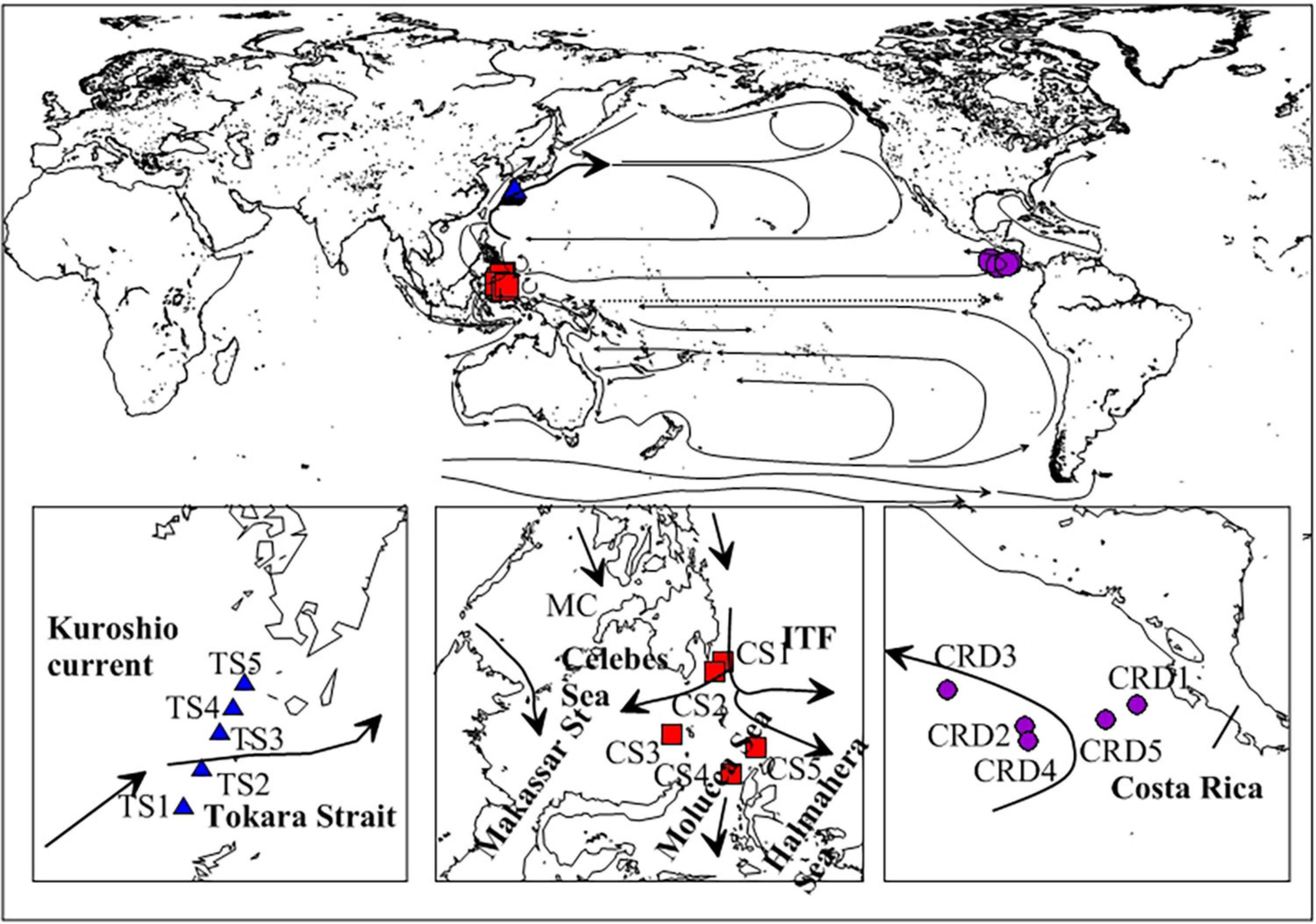
Figure 1. Locations of the sampling stations in three investigated regions around the Pacific Ocean, including Costa Rica Dome (CRD), Celebes Sea (CS), and Tokara Strait (TS; ITF, The Indonesian throughflow).
Sampling plans included: (1) Tintinnid samples in the CRD were conducted at 5 sites from June 25 to July 22 in 2010 (8°30′–10°8′ N, 86°52′–92°59′ W, Figure 1). At each site, 7 layers were sampled from 0 to 200 m: surface layer, surface mixed layer, the layer above Chl a max, Chl a max layer, layer below Chl a max, interface layer, and deep control layer. (2) Tintinnid samples in the CS were collected at 5 sites from November 30 to December 5 in 2012 (2°–6°12′ N, 124°50′–128° E, Figure 1). The sampling depths ranged from 0 to 200 m or 2 m up to the bottom: 5, 30, 50, 75, 100, 150, and 200 m. (3) Tintinnid samples in the TS were collected at 5 sites in December 2012 (29°0.1′–31°0.2′ N, 129°0.6′–130°0.1′ E, Figure 1). The sampling depths ranged from 0 to 200 m or 2 m above the bottom: 5, 30, 50, 100, and 200 m.
Sampling methods were similar in the three investigated regions. At each site, a 10, 20, or 30 L water sample was collected using Niskin bottles at each layer, and then filtered slowly and gently through a net (mesh size 20 μm). The concentrated samples (∼150 ml) were fixed with formalin solution to 5% final concentration and stored in adiaphanous plastic bottles in the lab. Tintinnid enumeration was conducted according to the method of Utermöhl (1958). Subsamples of 20 ml from well-mixed concentrated samples were pipetted into a sedimentation chamber and settled for 24 h, and subsequently counted under an Olympus IX 71 inverted microscope (200× or 400×) with a photographic measurement system.
Tintinnid species identifications were made on the basis of lorica morphology and dimensions according to literature (Kofoid and Campbell, 1929, 1939; Zhang et al., 2012; Santoferrara et al., 2017). Here we employed an approach (Dolan et al., 2006) to identification: any intermediate forms or slight variants were pooled with the morphologically closest and most numerous species. To measure the lorica oral diameter (LOD) and lorica length (LL), 10 to 20 individuals of each species were randomly picked and measured, and lorica volume (LV) was calculated. Species with rare occurrences were assigned the average dimensions reported in literatures as mentioned above.
Data Analysis
Water masses were distinguished by the temperature-salinity diagram based on Kato and Taniguchi (1993) and Gallager et al. (1996), with consideration of cluster analysis by PRIMER version 6.1 package (Clarke and Gorley, 2006). The tintinnid species pool in this study excluded species that only occurred once in the whole observation of total samples (strays and questionable species). Taxonomic diversity was estimated for each sample as species richness, which was represented by the total number of species in a sampling or in an investigated area. Based on Dolan et al. (2009), species were classified as “core species,” found in all the three investigated regions, or “common species,” which indicates occurrence in two investigated regions, or “endemic species” which only occurred in one area. Abundant species herein was defined as species that occupied >5% of the total abundance. Carbon biomass (C) was estimated using the equation: C = 444.5 + 0.053 × LV (Verity and Langdon, 1984).
Morphological diversity was estimated by placing species into size classes of LOD, which indicates ecological role relative to preferred prey size (Dolan, 2010). Size-class diameters were binned over 4 μm intervals beginning with the smallest diameter encountered and continuing to the overall largest specimen (Dolan et al., 2006; Dolan, 2010). Species occupying a size-class along with one or more other species were defined as “ecological redundants” and the number of size-classes containing more than one species was given as size-classes co-habitated (Dolan et al., 2016). Tintinnid genera were assigned to different biogeographic distribution patterns according to Dolan et al. (2013).
We calculated the mean abundance for each species, ranked from highest to lowest. Species abundance distribution (SAD) was used to describe the variation of abundance for each species ranked from highest to lowest (Dolan et al., 2007; Zhang et al., 2017). SADs were fitted with 4 common distribution models by the maximum likelihood method with the following numerical optimization: geometric, log-normal, log-series, and mZSM distribution. Fitting of the models and Akaike’s information criterion (AIC) were carried out using the sads package in the R program. Principal coordinate analysis (PCoA) was performed to explore the spatial variations of tintinnid assemblages, and redundancy analysis (RDA) was conducted to explore the relationships between tintinnid assemblages and abiotic factors using the R program. Univariate correlation analyses were carried out using the statistical program SPSS version 13.0 to explore the Pearson relationships between biotic variables across all sites. An ANOVA test (5% significance level) was used to test differences of tintinnid abundances (log-transformed) between seasons and regions by SPSS version 13.0.
To reveal the tintinnids migration among the three investigated regions through the Pacific Ocean, the migration simulation of the Lagrangian model was built using an off-line run of the MITgcm (MIT general circulation model) floats package1 as used in Shropshire et al. (2021) forced with three-dimensional circulation from the global HYCOM reanalysis GLBv0.08 product (Chassignet et al., 2007; Cummings and Smedstad, 2013). Results were analyzed with Matlab version 2020b. A total of 43,800 particles were released from the three regions at 8 depths with passive dispersal for a time span of 20 years and sampled with a 10-day interval.
Results
General Hydrology
Environmental factors were different in the three investigated regions (Figure 2). The temperature ranged from 11.97 to 28.51 (18.59 ± 5.96)°C, 13.55 to 29.18 (24.42 ± 4.94)°C, and 12.75 to 24.40 (21.91 ± 3.27)°C in the CRD, CS, and TS, respectively. Salinity fell in the ranges of 33.45–34.93 (34.51 ± 0.54), 31.55–35.13 (34.14 ± 1.48), and 34.14–34.86 (34.44 ± 0.17) in the CRD, CS, and TS, respectively. Chl a in vivo fluorescence ranged from 0.10 to 1.22 (0.53 ± 0.28), 0.04–1.01 (0.22 ± 0.22), and 0.05–0.84 (0.37 ± 0.24) in the CRD, CS, and TS, respectively. Chl a values were highest in the CRD. With consideration of water depths and cluster analysis, four water masses were distinguished by the temperature-salinity diagram in each of the three sampling regions (Figure 2A).
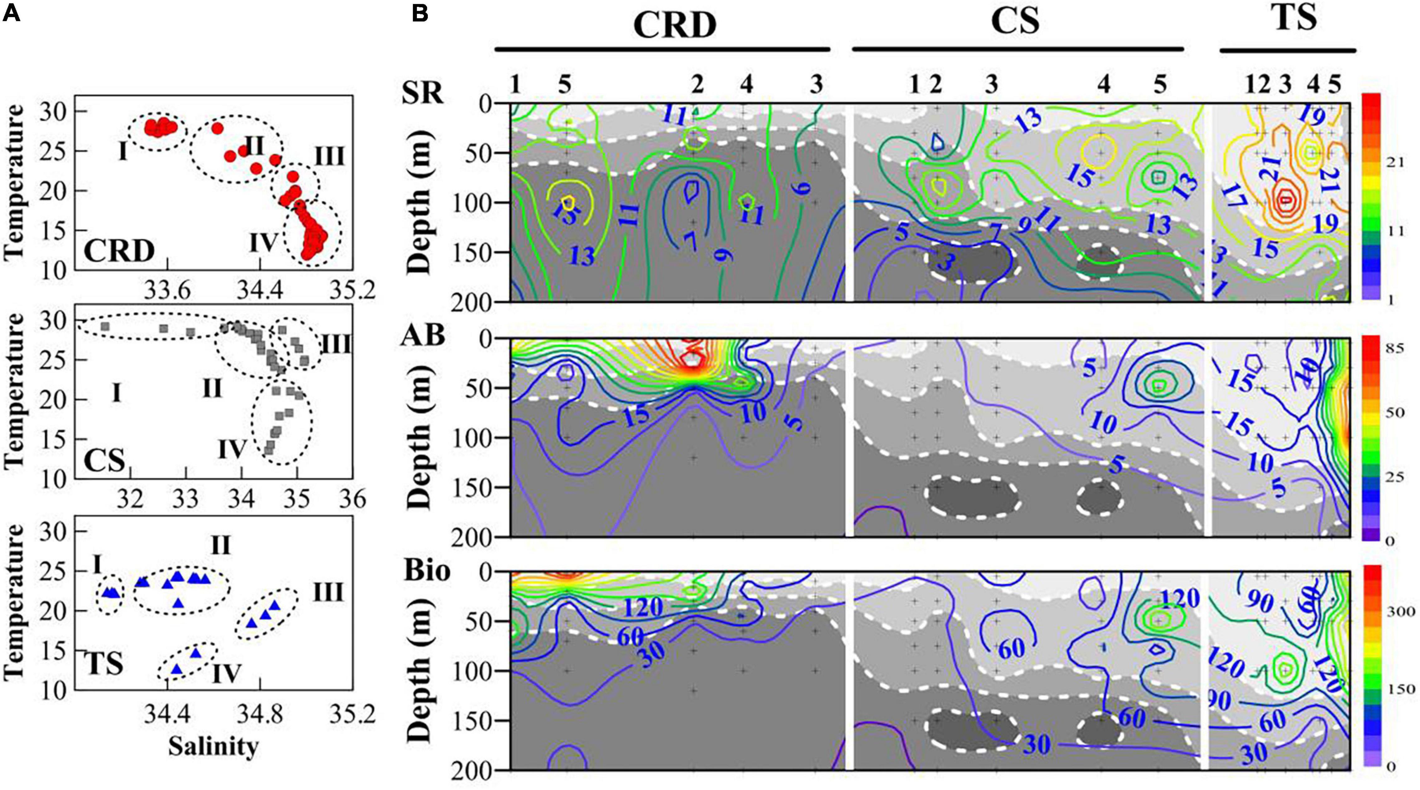
Figure 2. (A) Different water masses were identified from temperature-salinity diagrams with consideration of cluster analysis for the three investigated regions: CRD, CS, and TS, I–IV indicates four water masses in each of the three investigated regions. (B) Vertical distribution of species richness (SR), abundance (AB, × 103 ind m–3), and biomass (Bio, μg m–3) of tintinnid assemblages. White dotted lines show limits between different water masses defined in Panel (A).
General Tintinnid Assemblages
In total, 46 species of tintinnids were found across the three investigated regions (Table 1), with a total of 37, 38, and 34 species in the CRD, CS, and TS, respectively. Total tintinnid abundances and biomass ranged 533–93,624 ind m–3 (2.2–372.9 μg C m–3 for biomass) in the CRD, 100–35,600 ind m–3 (0.2–238.8 μg C m–3) in the CS, and 2,200–69,400 ind m–3 (13.1–263.7 μg C m–3) in TS, respectively. Tintinnid assemblages in the CS had the largest species number, but were lowest in both abundances and biomass (Figure 2B). Log-transformed abundances followed a normal distribution. ANOVA with main effects (regions and seasons) without interaction showed clear effects on tintinnid assemblages for regions (p < 0.05) but not for seasons. Margalef’s species richness index (D) ranged 0.4–1.7 in the CRD, 0–2 in the CS, and 1.3–2.9 in the TS, respectively. Shannon diversity index (H’) ranged 1.2–2.6 in the CRD, 0–2.6 in the CS, and 2–2.8 in the TS, respectively. Pielou’s evenness index (J) ranged 0.6–1 in the CRD, 0.8–1 in the CS, and 0.7–0.9 in the TS, respectively.
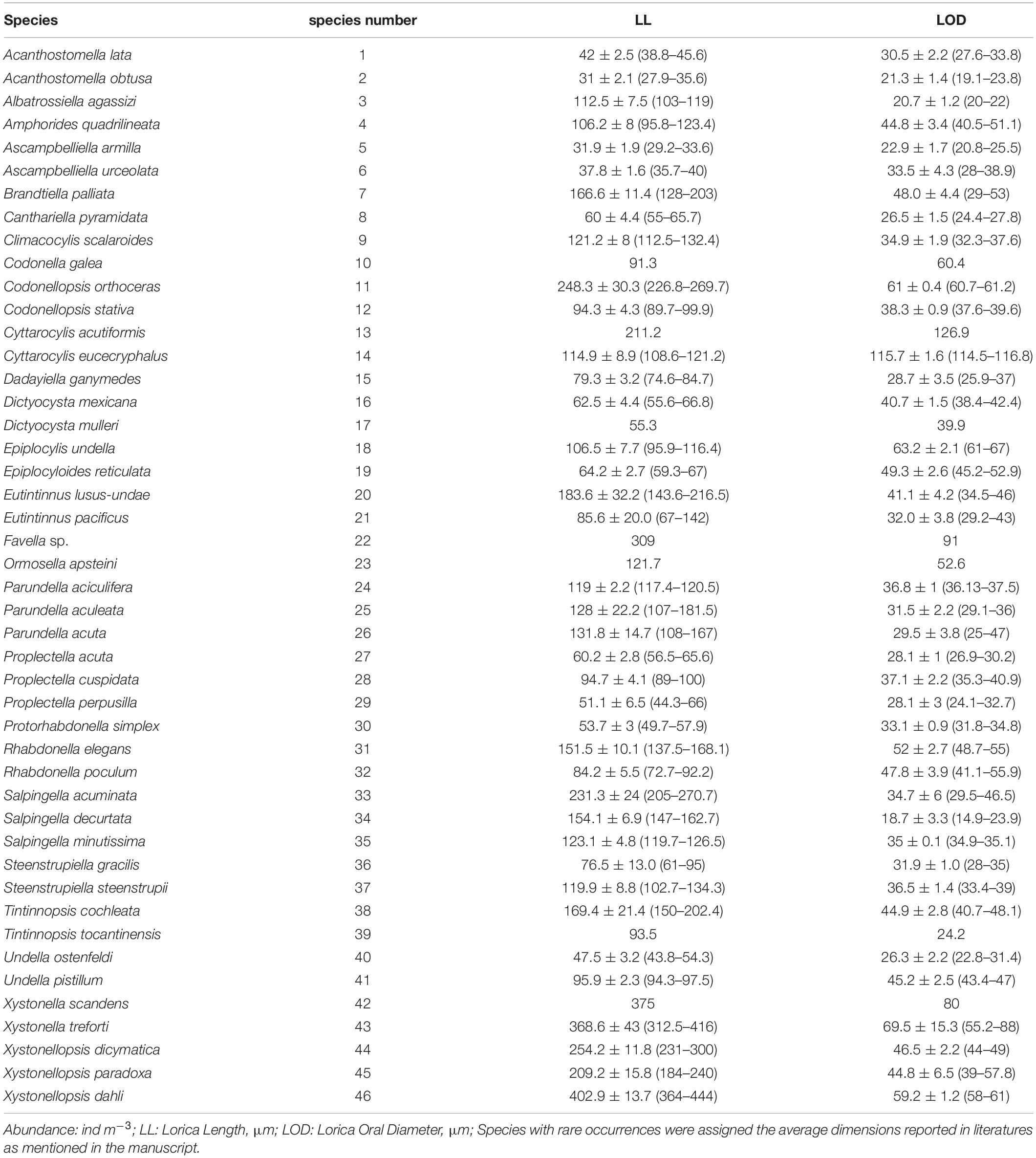
Table 1. Tintinnid species list and measurement data including lorica length and lorica oral diameter.
For all three investigated regions, maxima of tintinnid species richness and abundances always occurred in the upper two water masses (Figure 2B), although richness and abundance maxima were not always co-located, and high values were more likely to occur at the interface of different water masses. In the CRD, tintinnid abundances peaked in water mass CRDII at 20 m in St. CRD2 in relatively strong temperature gradients at interfaces between water masses, while biomass peaked in St. CRD5 due to the dominance shift from small individuals Ascampbelliella armilla to a larger species Rhabdonella elegans. In the CS, tintinnid species richness peaked in water mass CSII at St. CS4 and changed largely with low total abundances in the thermohaline intrusion in the upper 100 m in St. CS2 at the entrance of the CS. In the TS, tintinnid species richness and abundances peaked in water mass TSII especially in the intersection of different water masses where isotherms sloped sharply, whereas the least individuals were found in water mass IV. Tintinnid abundances in water mass TSI were consistently high while those in water mass TSIII were similarly low. When water mass intrusions were dramatic, tintinnid abundance decreased but species richness remained high.
Comparisons of Taxonomic Composition
For tintinnid assemblages in the three investigated regions, similar taxonomic compositions were revealed in terms of species, abundant species, genera, LOD size classes, and biogeographic patterns (Figure 3 and Tables 2, 3). A total of 29 species (63.0% of total species richness, Figure 3A) occurred in all three regions, i.e., core species, which significantly comprised 97.1% of the total abundances. These core species also occupied 77.8% of the total genera (21 genera out of 27, occupying 99.3% of total abundances, Figure 3B), and 81.3% of size-classes (13 out of 16, occupying 99.9% of total abundances, Figure 3C). In total, 5 common species and 12 endemic species were found in this study, although all their abundances were very low (<2,000 ind m–3, except Steenstrupiella gracilis). The overwhelming majority of core species indicated the numerically abundant forms remained more or less the same set of species in the three regions.
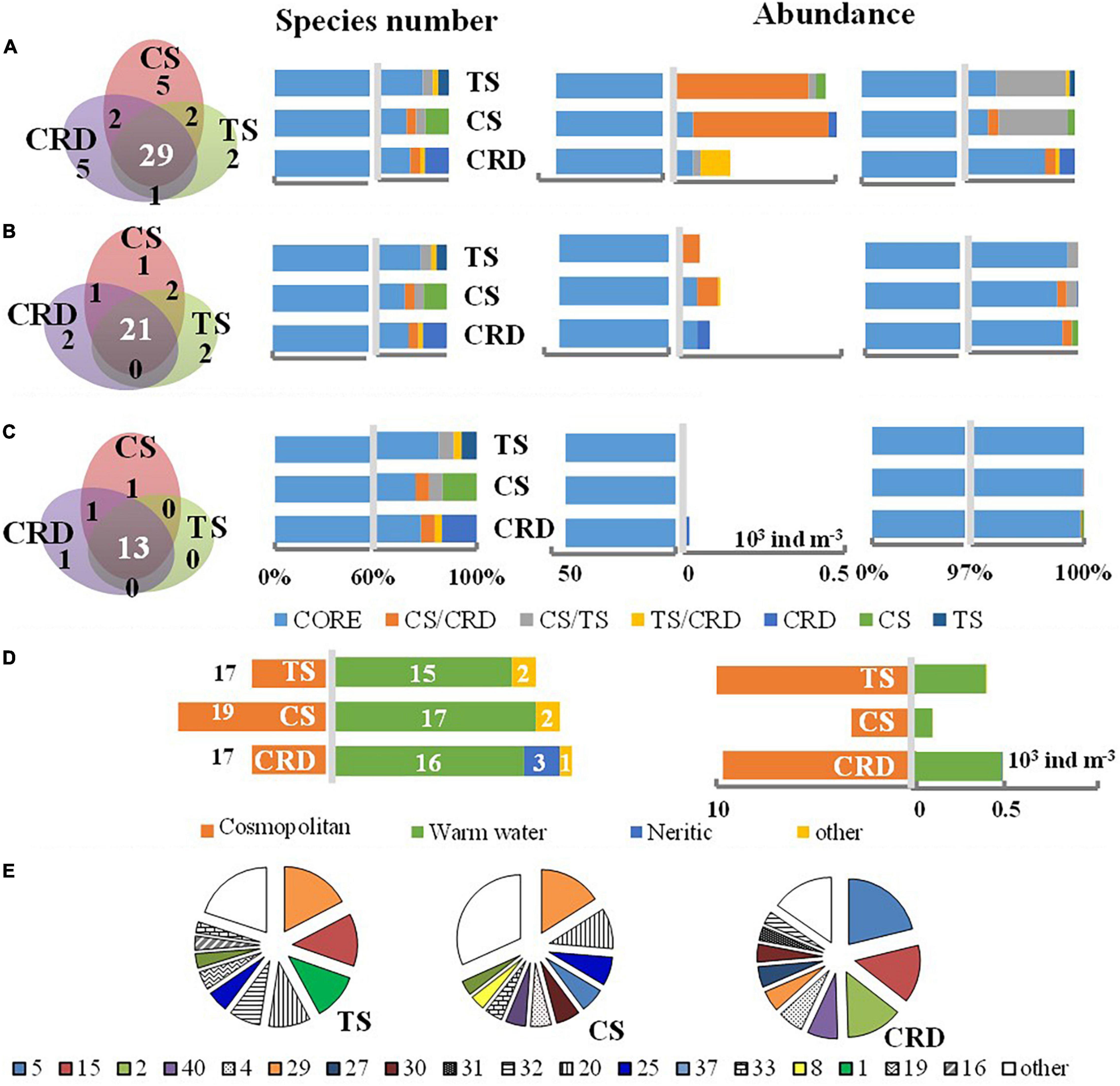
Figure 3. Comparisons of the taxonomic composition of tintinnid assemblages in terms of species (A), genera (B), LOD size-class (C), biogeographic patterns (D), and abundant species (E) in the CRD, CS, and TS, with consideration of species richness and abundances. Core (CORE), common (CS/CRD, CS/TS, and TS/CRD), and endemic species (CRD, CS, and TS) are shown in Panels (A–C). The abundance percentages of the first 10 abundant species are shown in Panel (E). Species numbers are shown in Table 1.
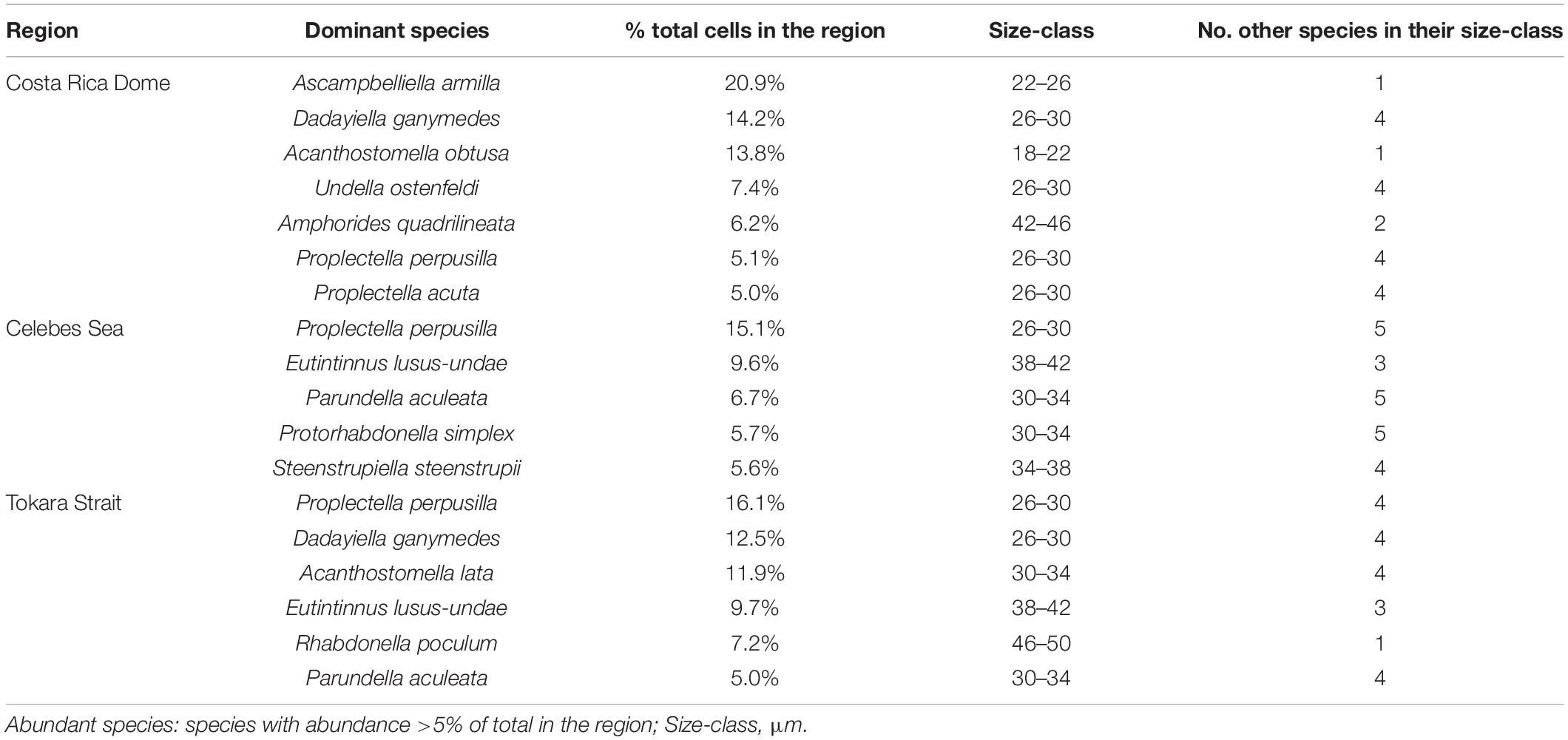
Table 2. Identity and morphology of the dominant species in the assemblages.
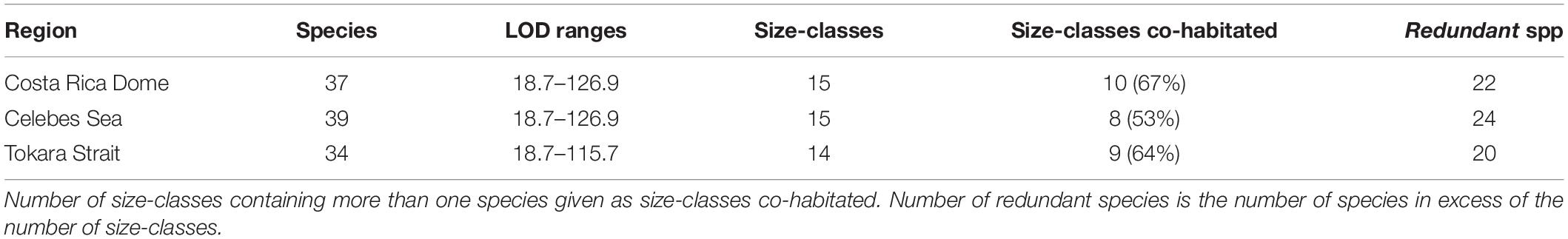
Table 3. Summary of morphological data by region.
Although abundant species were different (Table 2 and Figure 3E), all of them occurred as core species in the three regions. There were 7, 5, and 6 abundant species observed in samples of the CRD, CS, and TS, respectively. In all three regions, Proplectella perpusilla (P. perpusilla) was the numerically dominant species. There were 3 dominant species (P. perpusilla, Eutintinnus lususundae, and Parundella aculeate) in common between the TS and CS, and 2 dominant species (Dadayiella ganymedes and P. perpusilla) in common between the TS and CRD. However, tintinnids in the CRD had no dominant species in common with the CS, which was consistent with the largest distance between the two investigated regions. Abundances of all the dominant species were found significantly positively correlated to total abundances (p < 0.05).
Similar compositions of tintinnid assemblages were revealed among the three regions in terms of LOD size classes (Table 2 and Figure 3C). The LOD ranges and number of size-classes of all and co-habitated species were similar in the three regions (Table 3), and LOD size-class 26–30 μm contained the most redundant species and the largest proportion of total abundances (Figure 3C). Notably, tintinnid populations in the CRD were clearly distinguished from those in the CS and TS in LOD size classes for abundant species. Three out of 4 LOD size classes were the same in the CS and TS, while only one was the same as in the CRD. Redundants were most numerous in the size classes of the first dominant species in the CS and TS, but not in the CRD.
Three biogeographic distribution patterns were identified: cosmopolitan, warm-water, and neritic which occurred only in one site in the CRD nearest to the coast. All the core species were found as two biogeographic patterns: cosmopolitan (16 species) and warm-water (12 species). The two types occupied most of the species number with similar proportions, while abundances of the cosmopolitan type were higher than those of warm water in the TS and CS (Figure 3D). Endemic species of the three regions were revealed related to biogeographic types, i.e., endemic species were neritic, cosmopolitan, and warm-water species in the CRD, CS, and TS, respectively, with the addition of warm-water species in each area. The endemic species of the CRD were restricted to water masses CRDIII and CRDIV in the intermediate layer, while endemic species of the TS were restricted to water mass TSI and TSIII in the upper layer.
Comparisons of Community Structure
To explore the overall variability in community composition, we performed PCoA which revealed a clear separation between samples in the 0–50 m depth range and deeper depths (Figures 4A–C), and depth explained even more of the variance in terms of LOD size class. Furthermore, to explore the relationships between abiotic factors and tintinnids, we conducted RDA analysis and found clear distinctions among samples from different water depths, especially in terms of LOD size-class (Figures 4E,E1, r2 = 0.59, p < 0.01). Samples above 100 m were clearly distinguished from those below 100 m (Figures 4E1,F1). Water depth was negatively correlated tintinnid species richness and abundance (p < 0.05). Clear distinctions were also revealed by RDA analysis among tintinnid assemblages in the three regions in terms of species and genera (Figures 4D,F,D1,F1), while tintinnid assemblages in the TS were aggregated and close to those in the CS in terms of LOD size-class (Figure 4E). The latitudinal decline of tintinnid species richness (Dolan et al., 2016) was evident in the case of the CRD (r = −0.359, p < 0.05) and the CS (r = −0.302, p < 0.05), but not in the TS. Temperature and Chl a were positively correlated with tintinnid species richness and abundances (p < 0.01).
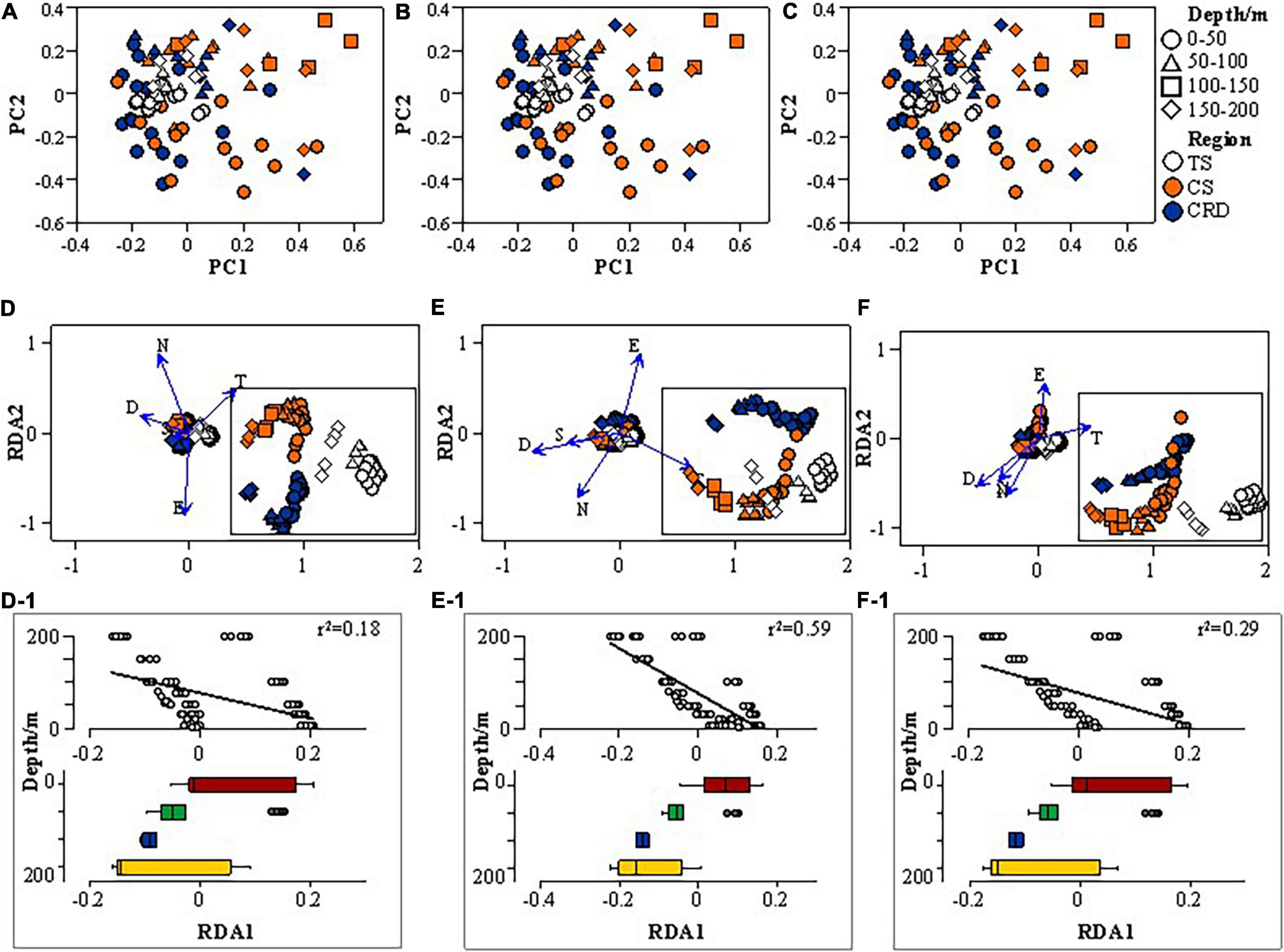
Figure 4. Principal coordinate (PC) analysis performed on community composition dissimilarities (Bray-Curtis) of tintinnid samples in the CRD, CS, and TS in terms of species (A) and LOD size-class (B), and genera (C), and RDA analysis performed on the abiotic factors (E, longitude; N, latitudinal; D, Depth; T, Temperature; S, Salinity) in the three investigated regions in terms of species (D) and LOD size-class (E), and genera (F), with consideration of depth. Boxplots (D-1–F-1) of the first PC illustrate differences between depth layers.
Species abundance distribution was fitted to the geometric, log-normal, log-series, and mZSM distributions by the AIC statistic (Table 4 and Figure 5). The log-normal distribution provided the best match to the observed pattern in the CRD and TS while the geometric distribution gave the best fit in the CS both in terms of species and LOD size-class. The AIC values of the geometric distribution in the CS were very close to those of log-normal distributions. The geometric series, describing a sequential monopolization of resources, described well the tintinnid assemblages in the CS, which were warmest, with largest species richness but least abundance, and highly dominated by Proplectella perpusilla and Eutintinnus lususundae. The log-normal distribution, thought to result from complex species interactions, provided the best fit for the CRD and TS. For most sites, the observed distribution most closely matched log-series, coherent with the neutral theory of random colonization from a large species pool.
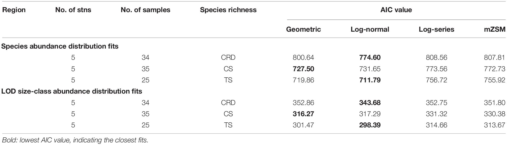
Table 4. Results of the analysis of tintinnid species abundance distribution (SAD) and LOD size-class abundance distribution in the Costa Rica Dome (CRD), Celebes Sea (CS), and Tokara Strait (TS). LOD: lorica oral diameter; AIC: Akaike’s information criterion; mZSM: meta-community zero-sum multinominal.
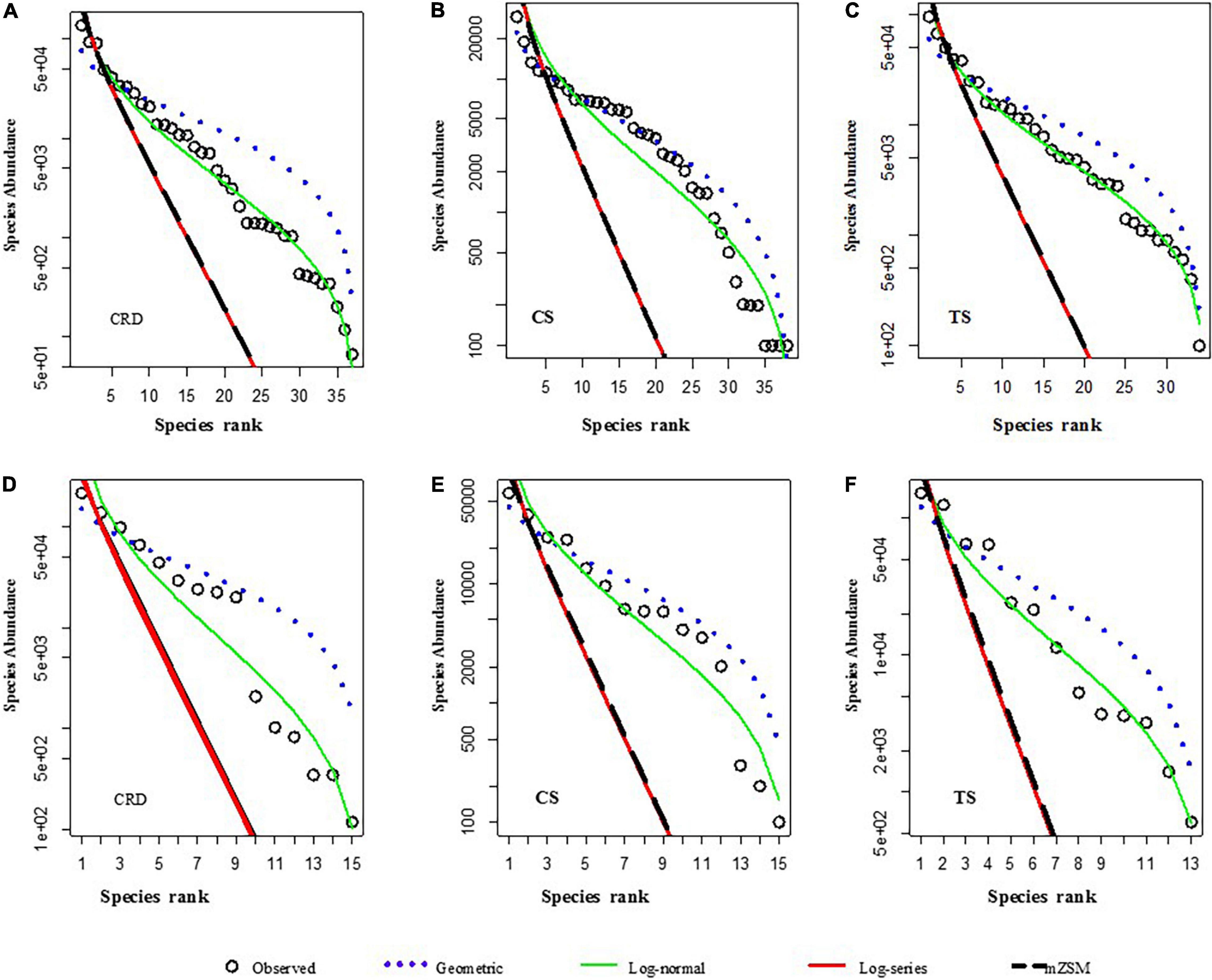
Figure 5. Species abundance distribution (A–C) and LOD size-class abundance distribution (D–F) of tintinnid populations in the CRD, CS, and TS. For species abundance distribution, the geometric distribution gave the best fit in CS (B), and the log-normal distribution provided the best fit for the CRD (A) and TS (C). For LOD size-class abundance distribution, the geometric distribution gave the best fit in the CS (E), and the log-normal distribution provided the best fit for the CRD (D) and TS (F). Actual observed abundances are shown in circles, and lines are the expected abundance from 4 theoretical distributions, MZSM: meta-community zero-sum multinomial.
Tintinnids Migration Simulation
We hypothesized that the greater similarity between tintinnid populations in the CS and TS (relative to CRD) was the result of geographical proximity and circulation patterns that link these regions. Lagrangian simulations (Supplementary Figure 1) revealed that it took the particles ≥710 days to migrate from the CS to CRD and ≥450 days to travel from the CRD to the CS, which approaches the cycle time of Pacific Equatorial Countercurrent. Thus, the result supported our hypothesis that tintinnid population could migrate across the Pacific Ocean near the equator, and they are more likely moving from the CS to CRD. Transit time from the CS to TS was ≥160 days (≥420 days from TS to CS), while it required ≥1,670 days for ciliates to be advected from the TS to CRD and 1,870 days from CRD to TS. With consideration of the Kuroshio Current and Mindanao Current, we deduced that tintinnids should migrate from someplace between the two currents, and migrate to the TS along with Kuroshio Current and the CS along with the Mindanao Current and then reach the CRD along with the Pacific Equatorial Countercurrent.
Discussion
Tintinnid Assemblages Migration in the Open Sea
What are the basin-scale relationships among the tintinnid assemblages as evidenced by the data from three different regions in this study? Based on the distance and ocean currents, we may have three possible scenarios. The first one is that tintinnid populations might migrate from the CRD to CS along with the North Equatorial Current and then to the TS along with the Kuroshio Current. Alternatively, tintinnid populations in the CS and TS might derive from the same origin or share a similar community structure, whereas tintinnids migration from the CRD to the other two regions is questionable. The third scenario is that there is no similarity among those tintinnid populations in the three regions. Comparisons of taxonomic compositions in terms of species, abundant species, LOD size classes, and genera supported the second scenario. Kim et al. (2012b) revealed tintinnids as bioindicators that more sensitively detected water mass extension and intrusion than physical properties. El-Serehy et al. (2014) reported the Suez Canal as a selective barrier and/or as a link in the migration of tintinnid protozoa. Li et al. (2016) excavated the interactions between different tintinnids in different water masses.
While our simple Lagrangian model allowed us to quantify advection patterns that potentially link these study regions, several points could be included in future-focused models: (1) the growth, death, and predation and life cycle of tintinnids could be explicitly models to assay community turnover and thus the succession of tintinnid communities during transit; (2) species growth responses to environmental variables could be included to differentiate between the importance local growth and advective processes in maintaining species patterns and determine the differences between “invasion” verse “migration” for the advected species competing with local species; and (3) the effects of chaotic advection by oceanic currents on biodiversity patterns of rare protist species could be investigated (mentioned by Martin et al., 2020).
Advantages of Tintinnids as Bioindicator in the Open Ocean
Plankton carried by the current often have distinct environmental niches and remain recognizable until they die and disintegrate, which make them reliable indicators of water mass movements (Kim et al., 2012a,b). The reliability of an indicator species is determined by the higher frequency of occurrence in a particular water mass and by identifiable morphology. The indicator species must be resistant to gradual changes in water properties (Schwenke, 1971), but should not be sufficiently capable of survival over a wide range of the change (Raymont, 1980; Kato and Taniguchi, 1993). Thus, with hard lorica, tintinnids are a reliable indicator of water mass movements (e.g., Kato and Taniguchi, 1993; Kim et al., 2012a,b; El-Serehy et al., 2014; Li et al., 2016), and information from tintinnid biological indicators was suggested to support physical oceanographic data to confirm ambiguous water mass properties (Kim et al., 2012a).
The hard loricae outside the tintinnids can remain even after their death making tintinnids even more effective as bioindicator of large-scale currents. Empty loricae of tintinnids have been used as indicators for tracing the movement of water masses and currents because their sinking rate, as well as decomposition rate, can be assumed to be very slow (Taniguchi, 1983; Kato and Taniguchi, 1993; Pierce and Turner, 1993; Suzuki and Taniguchi, 1995). Empty loricae were transported long distances by currents before settling to the sediments (Echols and Fowler, 1973). On the other hand, when loricae were found empty or damaged, this might indicate long-distance transport. Conversely, when loricae occupied by a living ciliate were observed, it was likely that the species lived either at or near the sampling site (Kim et al., 2012b). In this regard, the proportion of empty or damaged loricae was suggested as a useful property in tintinnid investigation in the open sea. However, there are limitations for tintinnids usage as bioindicators: the absence of standardization of the sampling methods, fixation method and analytical protocols, discrepancy of different identification schemes in the literature, as well as several highly polymorphic genera and the fact that criteria for the delimitation of the species may vary among the observers (Gómez, 2007).
Tintinnid Distribution at Micro/Meso-Scales
Gómez (2007) recorded 42 tintinnid species with low density (> 10 ind l–1 from Figures) in the CS and vicinity, while abundance was about 20–30 cells l–1 in the south of the Kuroshio Current. This study revealed similar results in the CS (Taniguchi, 1977) and in the CRD (Freibott et al., 2016), and higher abundance in the TS than those in the south of Kuroshio Current (Gómez, 2007). The assemblage of abundant species in the CRD appeared distinct from those abundant species of the CS and TS in terms of LOD size classes, presumably reflecting exploitation of different sizes of prey items. Many factors influencing tintinnid abundance have been discussed, including temperature, salinity, Chl a (e.g., Wang et al., 2018), water masses, latitude (Dolan et al., 2016), copepod nauplii and bottom depth (Santoferrara et al., 2011), mutualistic diatoms (Vincent et al., 2018), food conditions (Kazama and Urabe, 2016), etc. Most of these factors were assessed at micro-scales, while this study provided the possibility and practicability of quantifying tintinnid variation at the meso-scale. As Woods (1999) mentioned, we still cannot explain quantitatively how the relative abundance of plankton species varies geographically.
Redundant species were more common in the CS in low latitude than other regions, while warm-water species decreased with increasing latitude, providing a possible explanation of the latitudinal decline of tintinnid species richness. Redundants were most numerous in the size classes of the dominant species and can likely replace a dominant species, a result that is consistent with Dolan et al. (2016).
Species abundance distributions describe community structure and are a key component of biodiversity theory and research (Antão et al., 2021) and have been conducted on tintinnids in several previous studies (Dolan et al., 2016; Zhang et al., 2017). It was generally accepted that most distributions of species abundance in large assemblages are log-normally distributed (Gaston and Blackburn, 2000; Magurran and Henderson, 2003). This study showed that a log-normal distribution provided the best fit for tintinnid abundance distribution in the CRD and TS although a geometric distribution was the best fit in the CS both in terms of species and LOD size-class. Geometric distributions of LOD size-class abundance are most simply attributed to the availability of prey concentration and size given the close relationship between LOD size and prey exploited by tintinnids (Dolan, 2010). Geometric distribution mainly occurs in species-poor and often harsh environments (Magurran, 1988; Fattorini, 2005), or in the very early stages of succession (Whittaker, 1972; Matthews and Whittaker, 2015). The potential of the elucidation of macroscale species abundance has far been an inaccessible but critical property of biodiversity (Fukaya et al., 2020). Several theories have been involved in the SAD, including at different scales—the Neutral Theory of Biodiversity (NTB; Hubbell, 2001) and the Maximum Entropy Theory of Ecology (METE; Harte et al., 2008), and supporting or disproving these and other theories will require more studies that quantify the species distributions of plankton in the open seas.
Conclusion
1. More than half (64.0%) of tintinnid species were found in all three regions (144° longitude apart) around the North Pacific Ocean, accounting for 97.1% of total abundances, which indicated that the numerically abundant forms remain more or less the same set of species in the three regions.
2. Tintinnid community structure analyses, with respect to species, LOD, and genera, revealed clear distinctions among different regions and water depths, while tintinnid assemblages in the TS were closer to those in the CS than those in the CRD. Consequently, species occurrences changed remarkably, although the abundant tintinnid species were the same.
3. The Lagrangian simulation showed tintinnid migration in ocean currents across the Pacific Ocean, supporting the hypothesis that ocean circulation explains the similarity in tintinnid populations in the CS and TS, and that these are probably derived from the same origin, and are clearly distinct from those in the CRD.
Data Availability Statement
The original contributions presented in the study are included in the article/Supplementary Material, further inquiries can be directed to the corresponding authors.
Author Contributions
CW, WZ, HoL, and MF contributed to the conception, design, and development of the study. SL, SC, and HaL collected the samples on board and contributing authors participated in the collection of data. MF conducted samples identification and counting. WZ validated the species identification. MS, JI, and NL completed the simulation model. All authors approved the final version of the manuscript.
Funding
This study was supported by the National Science Foundation of China (NSFC Nos. 41806160 and 41706192), the Science and Technology Development Program of Shanghai Ocean University (A2-2006-21-200319 and A2-2006-20-200207), and the China Ocean Mineral Resources Research and Development Association Program (DY135-E2-3-4).
Conflict of Interest
The authors declare that the research was conducted in the absence of any commercial or financial relationships that could be construed as a potential conflict of interest.
Publisher’s Note
All claims expressed in this article are solely those of the authors and do not necessarily represent those of their affiliated organizations, or those of the publisher, the editors and the reviewers. Any product that may be evaluated in this article, or claim that may be made by its manufacturer, is not guaranteed or endorsed by the publisher.
Acknowledgments
We want to acknowledge the support of the crew of onboard the R/V Tansei Maru (JAMSTEC), R/V Melville, and R/V Kexue I.
Supplementary Material
The Supplementary Material for this article can be found online at: https://www.frontiersin.org/articles/10.3389/fmars.2022.863549/full#supplementary-material
Footnotes
References
Antão, L. H., Magurran, A. E., and Dornelas, M. (2021). The shape of species abundance distributions across spatial scales. Front. Ecol. Evol. 9:626730. doi: 10.3389/fevo.2021.626730
Azam, F., Fenchel, T., Field, J. G., Gray, J. S., Meyer-Reil, L. A., and Thingstad, F. (1983). The ecological role of water-column microbes in the sea. Mar. Ecol. Prog. Ser. 10, 257–263. doi: 10.3354/meps010257
Chassignet, E. P., Hurlburt, H. E., Smedstad, O. M., Halliwell, G. R., Hogan, P. J., Wallcraft, A. J., et al. (2007). The HYCOM (HYbrid Coordinate Ocean Model) data assimilative system. J. Mar. Sys. 65, 60–83. doi: 10.1016/j.jmarsys.2005.09.016
Christaki, U., Georges, C., Genitsaris, S., and Monchy, S. (2015). Microzooplankton community associated with phytoplankton blooms in the naturally iron-fertilized Kerguelen area (Southern Ocean). FEMS Microbiol. Ecol. 91:fiv068. doi: 10.1093/femsec/fiv068
Cummings, J. A., and Smedstad, O. M. (2013). “Variational data assimilation for the global ocean,” in Data Assimilation for Atmospheric, Oceanic and Hydrologic Applications, eds S. Park and L. Xu, (Berlin: Springer), Vol. II, 303–343.
Davis, C. S., Flierl, G. R., Wiebe, P. H., and Franks, P. J. S. (1991). Micropatchiness, turbulence and recruitment in plankton. J. Mar. Res. 49, 109–151. doi: 10.1357/002224091784968602
Dolan, J. R. (2010). Morphology and ecology in tintinnid ciliates of the marine plankton: correlates of lorica dimensions. Acta Protozool. 49, 235–244. doi: 10.1186/1471-2105-11-2
Dolan, J. R., and Marro, S. (2020). A note on the differences found between examining whole water vs. phytoplankton net (52 μm mesh) samples to characterize abundance and community composition of tintinnid ciliates (marine microzooplankton). Limnol. Oceanogr. Methods 18, 163–168. doi: 10.1002/lom3.10348
Dolan, J. R., Jacquet, S., and Torreton, J. P. (2006). Comparing taxonomic and morphological biodiversity of tintinnids (planktonic ciliates) of New Caledonia. Limnol. Oceanogr. 51, 950–958. doi: 10.2307/3841102
Dolan, J. R., Montagnes, D. J., Agatha, S., Coats, D. W., and Stoecker, D. K. (2013). The Biology and Ecology of Tintinnid Ciliates: Models for Marine Plankton. Hoboken, NJ: Wiley-Blackwell.
Dolan, J. R., Ritchie, M. E., and Ras, J. (2007). The “neutral” community structure of planktonic herbivores, tintinnid ciliates of the microzooplankton, across the SE Tropical Pacific Ocean. Biogeoscience 4, 297–310. doi: 10.5194/bg-4-297-2007
Dolan, J. R., Ritchie, M. E., Tunin-Ley, A., and Pizay, M. D. (2009). Dynamics of core and occasional species in the marine plankton: tintinnid ciliates in the north-west Mediterranean Sea. J. Biogeogr. 36, 887–895. doi: 10.1111/j.1365-2699.2008.02046.x
Dolan, J. R., Yang, E. J., Kang, S. H., and Rhee, T. S. (2016). Declines in both redundant and trace species characterize the latitudinal diversity gradient in tintinnid ciliates. ISME J. 10, 2174–2183. doi: 10.1038/ismej.2016.19
Echols, R. J., and Fowler, G. A. (1973). Agglutinated tintinnid loricae from some recent and late pleistocene shelf sediments. Micropaleontology 19, 431–442.
El-Serehy, H. A., Al-Misned, F. A., Abdel-Rahman, N. S., and Al-Rasheid, K. A. (2014). Tintinnids (Ciliophora: Choreotrichia) of the Suez Canal and their transmigration process between the Red Sea and the Mediterranean Sea. Aquat. Ecosyst. Health Manag. 17, 454–462. doi: 10.1080/14634988.2014.979601
Fattorini, S. (2005). A simple method to fit geometric series and broken stick models in community ecology and island biogeography. Acta Oecol. 28, 199–205. doi: 10.1016/j.actao.2005.04.003
Feng, M. P., Zhang, W. C., Wang, W. D., Zhang, G. T., Xiao, T., and Xu, H. L. (2015). Can tintinnids be used for discriminating water quality status in marine ecosystems? Mar. Pollut. Bull. 101, 549–555. doi: 10.1016/j.marpolbul.2015.10.059
Fiedler, P. C. (2002). The annual cycle and biological effects of the Costa Rica Dome. Deep Sea Res. 49, 321–338. doi: 10.1016/S0967-0637(01)00057-7
Forster, D., Bittner, L., Karkar, S., Dunthorn, M., Romac, S., Audic, S., et al. (2015). Testing ecological theories with sequence similarity networks: marine ciliates exhibit similar geographic dispersal patterns as multicellular organisms. BMC Biol. 13:16. doi: 10.1186/s12915-015-0125-5
Freibott, A., Taylor, A. G., Selph, K. E., Liu, H., Zhang, W., and Landry, M. R. (2016). Biomass and composition of Protistan grazers and heterotrophic bacteria in the Costa Rica Dome during summer 2010. J. Plankton Res. 38, 230–243. doi: 10.1093/plankt/fbv107
Fukaya, K., Kusumoto, B., Shiono, T., Fujinuma, J., and Kubota, Y. (2020). Integrating multiple sources of ecological data to unveil macroscale species abundance. Nat. Commun. 11:1695. doi: 10.1038/s41467-020-15407-5
Gallager, S. M., Davis, C. S., Epstein, A. W., Solow, A., and Beardsley, R. C. (1996). High-resolution observations of plankton spatial distributions correlated with hydrography in the Great South Channel, Georges Bank. Deep Sea Res. Top. Stud. Oceanogr. 43, 1627–1663. doi: 10.1016/S0967-0645(96)00058-6
Ganser, M. H., Forster, D., Liu, W., Lin, X., Stoeck, T., and Agatha, S. (2021). Genetic diversity in marine planktonic ciliates (Alveolata, Ciliophora) suggests distinct geographical patterns – data from Chinese and European Coastal Waters. Front. Mar. Sci. 8:643822. doi: 10.3389/fmars.2021.643822
Gómez, F. (2007). Trends on the distribution of ciliates in the open Pacific Ocean. Acta Oecol. 32, 188–202. doi: 10.1016/j.actao.2007.04.002
Grattepanche, J. D., McManus, G. B., and Katz, L. A. (2016). Patchiness of ciliate communities sampled at varying spatial scales along the New England shelf. PLoS One 11:e0167659. doi: 10.1371/journal.pone.0167659
Harte, J., Zillio, T., Conlisk, E., and Smith, A. (2008). Maximum entropy and the state-variable approach to macroecology. Ecology 89, 2700–2711. doi: 10.1890/07-1369.1
Haury, L. R., McGowan, J. A., and Wiebe, P. H. (1978). “Patterns and processes in the time-space scales of plankton distributions,” in Spatial Pattern in Plankton Communities, ed. J. H. Steele (New York: Plenum Press), 277–327.
Hu, D., Wu, L., Cai, W., Gupta, A. S., Ganachaud, A., Qiu, B., et al. (2015). Pacific western boundary currents and their roles in climate. Nature 522, 299–308. doi: 10.1038/nature14504
Hubbell, S. P. (2001). The Unified Neutral Theory of Biodiversity and Biogeography. Princeton, NY: Princeton University Press.
Jiang, Y., Xu, H. L., Hu, X. Z., Zhu, M. Z., Khaled, A. S., and Al-Rasheid, et al. (2011). An approach to analyzing spatial patterns of planktonic ciliate communities for monitoring water quality in Jiaozhou Bay, northern China. Mar. Pollut. Bull. 62, 227–235. doi: 10.1016/j.marpolbul.2010.11.008
Kato, S., and Taniguchi, A. (1993). Tintinnid ciliates as indicator species of different water masses in the western North Pacific. Fish. Oceanogr. 2, 166–174. doi: 10.1111/j.1365-2419.1993.tb00132.x
Kazama, T., and Urabe, J. (2016). Relative importance of physical and biological factors regulating tintinnid populations: a field study with frequent samplings in Sendai Bay, Japan. Mar. Freshwater Res. 67, 492–504. doi: 10.1071/MF14256
Kim, Y. O., Noh, J. H., Lee, T. H., Jang, P. G., Ju, S. J., and Choi, D. L. (2012a). Using tintinnid distribution for monitoring water mass changes in the Northern East China Sea. Ocean Polar Res. 34, 219–228. doi: 10.4217/OPR.2012.34.2.219
Kim, Y. O., Shin, K., Jang, P. G., Choi, H. W., Noh, J. H., Yang, E. J., et al. (2012b). Tintinnid species as biological indicators for monitoring intrusion of the warm oceanic waters into Korean coastal waters. Ocean Sci. J. 47, 161–172. doi: 10.1007/s12601-012-0016-4
Kofoid, C. A., and Campbell, A. S. (1929). A Conspectus of the Marine and Fresh Water Ciliata Belonging to Suborder Tintinnoinea, With Descriptions of New Species Principally from the Agassiz Expedition to the Eastern Tropical Pacific 1904-1905. Berkeley, CA: University of California Press.
Kofoid, C. A., and Campbell, A. S. (1939). Reports on the scientific results of the expedition to the eastern tropical Pacific, in charge of Alexander Agassiz, by the U.S. Fish Commission Steamer “Albatross”, from october 1904 to March 1905, Lieutenant Commander L.M. Garrett, U.S.N., commanding. XXXVII. The Ciliata: the Tintinnoinea. Bull. Mus. Comp. Zool. Harv. Coll. 84, 369–408. doi: 10.5962/bhl.part.27494
Li, H., Xuan, J., Wang, C., Chen, Z., Grégori, G., Zhao, Y., et al. (2021). Summertime tintinnid community in the surface waters across the North pacific transition zone. Front. Microbiol. 12:697801. doi: 10.3389/fmicb.2021.697801
Li, H., Zhao, Y., Chen, X., Zhang, W., Xu, J., Li, J., et al. (2016). Interaction between neritic and warm water tintinnids in surface waters of East China Sea. Deep Sea Res. Top. Stud. Oceanogr. 124, 84–92. doi: 10.1016/j.dsr2.2015.06.008
Li, W. K. W., Rao, S., Harrison, W. G., Smith, J. C., Cullen, J. J., Irwin, B., et al. (1983). Autotrophic picoplankton in the tropical ocean. Science 219, 292–295. doi: 10.1126/science.219.4582.292
Liu, W., McManus, G. B., Lin, X., Huang, H., Zhang, W., and Tan, Y. (2021). Distribution patterns of ciliate diversity in the South China Sea. Front. Microbiol. 12:689688. doi: 10.3389/fmicb.2021.689688
Lynn, D. H. (2008). The Ciliated Protozoa: Characterization, Classification, and Guide to the Literature: (3rd). Berlin: Springer Verlag, doi: 10.1007/978-1-4020-8239-9
Magurran, A. E. (1988). Ecological Diversity and its Measurement. Princeton, NJ: Princeton University Press.
Magurran, A. E., and Henderson, P. A. (2003). Explaining the excess of rare species in natural species abundance distributions. Nature 422, 714–716. doi: 10.1038/nature01547
Marshall, S. M. (1973). Respiration and feeding in copepods. Adv. Mar. Biol. 11, 57–120. doi: 10.1016/S0065-2881(08)60268-0
Martin, P. V., Bucek, A., Bourguignon, T., and Pigolotti, S. (2020). Ocean currents promote rare species diversity in protists. Sci. Adv. 6:eaaz9037. doi: 10.1101/2020.01.10.901165
Matthews, T. J., and Whittaker, R. J. (2015). On the species abundance distribution in applied ecology and biodiversity management. J. Appl. Ecol. 52, 443–454. doi: 10.1111/1365-2664.12380
Olson, M. B., and Daly, K. L. (2013). Micro-grazer biomass, composition and distribution across prey resource and dissolved oxygen gradients in the far eastern tropical North Pacific Ocean. Deep Sea Res. Top. Stud. Oceanogr. 75, 28–38. doi: 10.1016/j.dsr.2013.01.001
Pierce, R. W., and Turner, J. T. (1993). Global biogeography of marine tintinnids. Mar. Ecol. Prog. Ser. 94, 11–26. doi: 10.3354/meps094011
Raymont, J. E. G. (1980). Plankton and productivity in the oceans. Q. Rev. Biol. 2, 456–475. doi: 10.1016/B978-0-08-021551-8.50016-4
Saito, M. A., Rocap, G., and Moffett, J. W. (2005). Production of cobalt binding ligands in a Synechococcus feature at the Costa Rica upwelling dome. Limnol. Oceanogr. 50, 279–290. doi: 10.4319/lo.2005.50.1.0279
Santoferrara, L. F., Alder, V. V., and Mcmanus, G. B. (2017). Phylogeny, classification and diversity of Choreotrichia and Oligotrichia (Ciliophora, Spirotrichea). Mol. Phylogenet. Evol. 112, 12–22. doi: 10.1016/j.ympev.2017.03.010
Santoferrara, L. F., Bachy, C., Alder, V. A., Gong, J., Kim, Y. O., Saccà, A., et al. (2016). Updating biodiversity studies in loricate protists: the case of the tintinnids (Alveolata, Ciliophora, Spirotrichea). J. Eukaryot. Microbiol. 63, 651–656. doi: 10.1111/jeu.12303
Santoferrara, L. F., Gomez, M. I., and Alder, V. A. (2011). Bathymetric, latitudinal and vertical distribution of protozooplankton in a cold-temperate shelf (southern Patagonian waters) during winter. J. Plankton Res. 33, 457–468. doi: 10.1093/plankt/fbq128
Schwenke, H. (1971). “Water movement: plants,” in Marine Ecology, ed. O. Kinne (London: Wiley-Interscience), 1091–1122.
Shropshire, T. A., Morey, S. L., Chassignet, E. P., Karnauskas, M., Coles, V. J., Malca, E., et al. (2021). Trade-offs between risks of predation and starvation in larvae make the shelf break an optimal spawning location for Atlantic bluefin tuna. J. Plankton Res. fbab041. doi: 10.1093/plankt/fbab041
Song, W., Xu, D., Chen, X., Warren, A., Shin, M. K., Song, W., et al. (2021). Overview of the diversity, phylogeny and biogeography of Strombidiid Oligotrich ciliates (Protista, Ciliophora), with a brief revision and a key to the known genera. Front. Microbiol. 12:700940. doi: 10.3389/fmicb.2021.700940
Suga, T., Kato, A., and Hanawa, K. (2000). North pacific tropical water: its climatology and temporal changes associated with the climate regime shift in the 1970s. Prog. Oceanogr. 47, 223–256. doi: 10.1016/S0079-6611(00)00037-9
Suzuki, T., and Taniguchi, A. (1995). Sinking rate of loricae of some common tintinnid ciliates. Fish. Oceanogr. 4, 257–263. doi: 10.1111/j.1365-2419.1995.tb00149.x
Taniguchi, A. (1977). Distribution of microzooplankton in the Philippine Sea and the Celebes Sea in summer, 1972. J. Oceanographical Soc. Japan 33, 82–89. doi: 10.1007/BF02110013
Taniguchi, A. (1983). Microzooplankton distribution along a transverse section crossing a marked oceanic front. Mer 21, 95–101.
Utermöhl, H. (1958). Zur Vervollkommnung der quantitativen Phytoplankton-Methodik. SIL Commun. 9, 1–38. doi: 10.1080/05384680.1958.11904091
Varotsos, C. A., Mazei, Y. A., Burkovsky, I., Efstathiou, M. N., and Tzanis, C. G. (2015). Climate scaling behaviour in the dynamics of the marine interstitial ciliate community. Theor. Appl. Climatol. 125, 439–447. doi: 10.1007/s00704-015-1520-0
Verity, P. G., and Langdon, C. (1984). Relationships between lorica volume, carbon, nitrogen, and ATP content of tintinnids in Narragansett Bay. J. Plankton Res. 6, 859–868. doi: 10.1093/plankt/6.5.859
Vincent, F. J., Colin, S., Romac, S., Scalco, E., Bittner, L., Garcia, Y., et al. (2018). The epibiotic life of the cosmopolitan diatom Fragilariopsis doliolus on heterotrophic ciliates in the open ocean. ISME J. 12, 1094–1108. doi: 10.1038/s41396-017-0029-1
Wang, C. F., Li, H. B., Zhao, L., Zhao, Y., Dong, Y., Zhang, W. C., et al. (2018). Vertical distribution of planktonic ciliates in the oceanic and slope areas of the western Pacific Ocean. Deep Sea Res. 167, 70–78. doi: 10.1016/j.dsr2.2018.08.002
Whittaker, R. H. (1972). Evolution and measurement of species diversity. Taxon 21, 213–251. doi: 10.2307/1218190
Woods, J. (1999). Understanding the ecology of plankton. Eur. Rev. 7, 371–384. doi: 10.1017/S1062798700004154
Yang, E. J., Hyun, J. H., Kim, D., Park, J., Kang, S. H., Shin, H. C., et al. (2012). Mesoscale distribution of protozooplankton communities and their herbivory in the western Scotia Sea of the Southern Ocean during the austral spring. J. Exp. Mar. Biol. Ecol. 428, 5–15. doi: 10.1016/j.jembe.2012.05.018
Zhang, C. X., Sun, J., Wang, D. X., Song, S. Q., Zhang, X. D., and Munir, S. (2017). Tintinnid community structure in the eastern equatorial Indian Ocean during the spring inter-monsoon period. Aquat. Biol. 26, 87–100. doi: 10.3354/ab00677
Zhang, W. C., Feng, M. P., Yu, Y., Zhang, C. X., and Xiao, T. (2012). An Illustrated Guide to Contemporary Tintinnids in the World. Beijing: Science Press.
Keywords: tintinnid communities, water mass, migration, micro/meso scale, North Pacific Ocean
Citation: Feng M, Lin S, Zhang W, Wang C, Liu H, Cheung S, Li H, Stukel MR, Irving JP and Li N (2022) Micro-/Meso-Scale Distinction and Horizontal Migration of Tintinnid (Ciliophora: Tintinnida) Assemblages in Three Regions Around the North Pacific Ocean. Front. Mar. Sci. 9:863549. doi: 10.3389/fmars.2022.863549
Received: 27 January 2022; Accepted: 14 February 2022;
Published: 25 March 2022.
Edited by:
Dongyan Liu, East China Normal University, ChinaReviewed by:
Dibyendu Rakshit, University of Calcutta, IndiaChih-Ching Chung, National Taiwan Ocean University, Taiwan
Copyright © 2022 Feng, Lin, Zhang, Wang, Liu, Cheung, Li, Stukel, Irving and Li. This is an open-access article distributed under the terms of the Creative Commons Attribution License (CC BY). The use, distribution or reproduction in other forums is permitted, provided the original author(s) and the copyright owner(s) are credited and that the original publication in this journal is cited, in accordance with accepted academic practice. No use, distribution or reproduction is permitted which does not comply with these terms.
*Correspondence: Chunsheng Wang, d2FuZy1zaW9AMTYzLmNvbQ==; Wuchang Zhang, d3VjaGFuZ3poYW5nQDE2My5jb20=