Evaluating the impacts of mesoscale eddies on abundance and distribution of neon flying squid in the Northwest Pacific Ocean

Mesoscale eddies are ubiquitous in global oceans yielding significant impacts on marine life. As a short-lived pelagic squid species, the population of neon flying squid (Ommastrephes bartramii) is extremely sensitive to changes in ambient oceanic variables. However, a comprehensive understanding of how mesoscale eddies affect the O. bartramii population in the Northwest Pacific Ocean is still lacking. In this study, a 10-year squid fisheries dataset with eddy tracking and high-resolution reanalysis ocean reanalysis data was used to evaluate the impact of mesoscale eddies and their induced changes in environmental conditions on the abundance and habitat distribution of O. bartramii in the Northwest Pacific Ocean. A weighted-based habitat suitability index (HSI) model was developed with three crucial environmental factors: sea surface temperature (SST), seawater temperature at 50-m depth (T_50m), and chlorophyll-a concentration (Chl-a). During years with an unstable Kuroshio Extension (KE) state, the abundance of O. bartramii was significantly higher in anticyclonic eddies (AEs) than that in cyclonic eddies (CEs). This difference was well explained by the distribution pattern of suitable habitats in eddies derived from the HSI model. Enlarged ranges of the preferred SST, T_50m, and Chl-a for O. bartramii within AEs were the main causes of more squids occurring inside the warm-core eddies, whereas highly productive CEs matching with unfavorable thermal conditions tended to form unsuitable habitats for O. bartramii. Our findings suggest that with an unstable KE background, suitable thermal conditions combined with favorable foraging conditions within AEs were the main drivers that yielded the high abundance of O. bartramii in the warm eddies.

1 Introduction

Neon flying squid (Ommastrephes bartramii) is a pelagic squid species extensively distributed in subtropical and temperate oceans. The North Pacific population of O. bartramii comprises two seasonal spawning cohorts (the winter-spring cohort and the autumn cohort) (Bower and Ichii, 2005). Both cohorts undergo meridional migrations between their spawning ground (subtropical frontal zone: 20–30°N) and feeding ground (Kuroshio–Oyashio transition and subarctic frontal zone: 30–50°N) within their 1-year lifespan (Murata, 1993). The importance of this species is underlined by its ecological significance as a structuring role to link different trophic levels (Watanabe et al., 2004), as well as its high commercial value to support international distant-water fisheries (Chen et al., 2008a). It is largely exploited by China (including Chinese Taipei), Japan, and Korea in the Northwest Pacific Ocean. Chinese squid-jigging fishing vessels mainly harvest the western stock of the winter-spring cohort of O. bartramii from July through November in the area bounded by 36°-48°N and 150°-165°E.

The subtropical and subpolar Northwest Pacific Ocean is dominated by two western boundary currents, the Kuroshio Current characterized as a warm and nutrient-poor current and the Oyashio Current characterized as a cold and nutrient-rich current. The Kuroshio-Oyashio transition zone with high biological productivity is an important feeding ground for many commercially important marine species including O. bartramii (Watanabe et al., 2008; Ohshimo et al., 2018; Ishak et al., 2020). Previous studies have suggested that the variability of the Kuroshio path can affect the abundance and distribution of O. bartramii (Shao et al., 2005; Chen et al., 2010a; Chen et al., 2012). The warm, northward-flowing waters of the Kuroshio Current separate from the Japanese coast to flow eastward into the North Pacific Ocean as a free jet-the Kuroshio Extension (KE) Current (Jayne et al., 2009). Based on the satellite altimeter measurement over the past decades, the interannual shifts of the KE path between a stable and an unstable dynamic state has been revealed (Qiu and Chen, 2005; Qiu and Chen, 2010). The impacts of this interannual variability of KE on eddy changes and marine primary production in the North Pacific Ocean have been emphasized by many studies (Lin et al., 2014; Yang et al., 2018). In addition, the impacts of the KE Current-related eddy changes on swordfish, a marine top predator, in the Northwest Pacific Ocean were pointed out by a recent study (Gómez et al., 2020).

Mesoscale eddies are ubiquitous in global oceans, ranging in size from tens to hundreds of kilometers with high energy (Chelton et al., 2011a). Eddies can be categorized as being either cyclonic eddies (cold-core; CE) or anticyclonic eddies (warm-core; AE), which rotate counterclockwise and clockwise in the northern hemisphere, respectively. Eddies modulate regional primary production through a variety of mechanisms, including vertical or horizontal advection of nutrients/phytoplankton, and regulation of light availability by changing ocean stratification (Gaube et al., 2014; McGillicuddy, 2016). Many studies have suggested that mesoscale eddies can attract a variety of marine organisms by providing foraging opportunities (Godø et al., 2012; Schmid et al., 2020) and favorable physical conditions (Gaube et al., 2018; Braun et al., 2019). CEs and AEs are known to have different effects on local marine ecosystems due to the opposite rotating direction and the accompanying opposite vertical movement pattern of water mass (Chelton et al., 2011b; Gaube et al., 2014). Typically, for most surface-intensified eddies, CE causes a vertical upward flow of seawater (upwelling) at its core and outward advection (divergence) at the surface. In contrast, AE causes downwelling at its core and convergent flow at the surface. Thus, CEs are generally considered to be productive due to the upwelling inside them, while AEs are considered to be unproductive ocean “deserts” (Gaube et al., 2014). The differences in the influence of CEs and AEs on biological communities, from plankton to predators, have been explored in numerous studies and have obtained diverse results (Gaube et al., 2014; Hsu et al., 2015; Gaube et al., 2018; Waite et al., 2019).

The KE Current is one of the most dynamic regions in the world’s oceans and contains highly energetic eddies that provide potential habitats for pelagic species (Polovina et al., 2006; Zainuddin et al., 2006). As for O. bartramii, it is believed that the existence of eddies is conducive to the formation of good fishing grounds (Chen, 1995). Sea surface height (SSH) and eddy kinetic energy (EKE), as two variables used to indicate ocean mesoscale dynamics, were widely applied to the evaluation of habitat patterns for O. bartramii (Chen et al., 2011; Yu et al., 2015; Yu et al., 2016). However, the variability and potentially different ecological roles of CEs and AEs cannot be comprehensively revealed by the two variables. A recent study using eddy identification methods suggested that the monthly squid habitat hotspots are likely associated with transient oceanic eddies, especially warm-core eddies (Alabia et al., 2015). The close association between the squid habitat and the eddies has not been confirmed, and the study region was limited to the central North Pacific.

Current knowledge of how the transient eddies affect O. bartramii stock in the Northwest Pacific Ocean is quite scattered. A comprehensive insight into the different roles of CEs and AEs in affecting the abundance and distribution of O. bartramii is still lacking. Based on a weighted-based habitat suitability index (HSI) model and data from 10-year long-term squid fisheries, eddies tracking, and high-resolution ocean reanalysis, this study evaluated the impacts of mesoscale eddies-induced changes in environmental conditions on the abundance and distribution of O. bartramii in the Northwest Pacific Ocean. The distinction between the impacts of cyclonic and anticyclonic eddies on an environment-sensitive squid species was emphasized.

2 Materials and methods

2.1 Fisheries data

The 10-year squid fisheries data between July and November from 2009 through 2018 used in this study were available from the Chinese Squid-jigging Science and Technology Group of Shanghai Ocean University. The study area was the main fishing ground of the western winter-spring cohort of O. bartramii in the Northwest Pacific Ocean bounded by 38–46°N and 145–165°E (Figure 1). The western winter-spring O. bartramii cohort was exploited by squid jigging fisheries without bycatch, and its catch accounted for most of the squid catches in the Northwest Pacific Ocean. Chinese squid-jigging vessels were equipped with an almost identical engine, lamp, and fishing power and all operated at night. The logbook information included fishing location (latitude and longitude), fishing date (year, month, and day), catch (tons), and fishing effort (in units of fishing days). Due to the homogeneous characteristics and operating behaviors of the Chinese squid-jigging vessels, Catch-per-unit-effort (CPUE) is regarded as a good indicator of O. bartramii stock abundance (Chen et al., 2008b). The CPUE was calculated as follows:

$$\text{CPUE}=\frac{{\sum }^{}\text{Catch}}{{\sum }^{}\text{Fishing effort}}$$

FIGURE 1

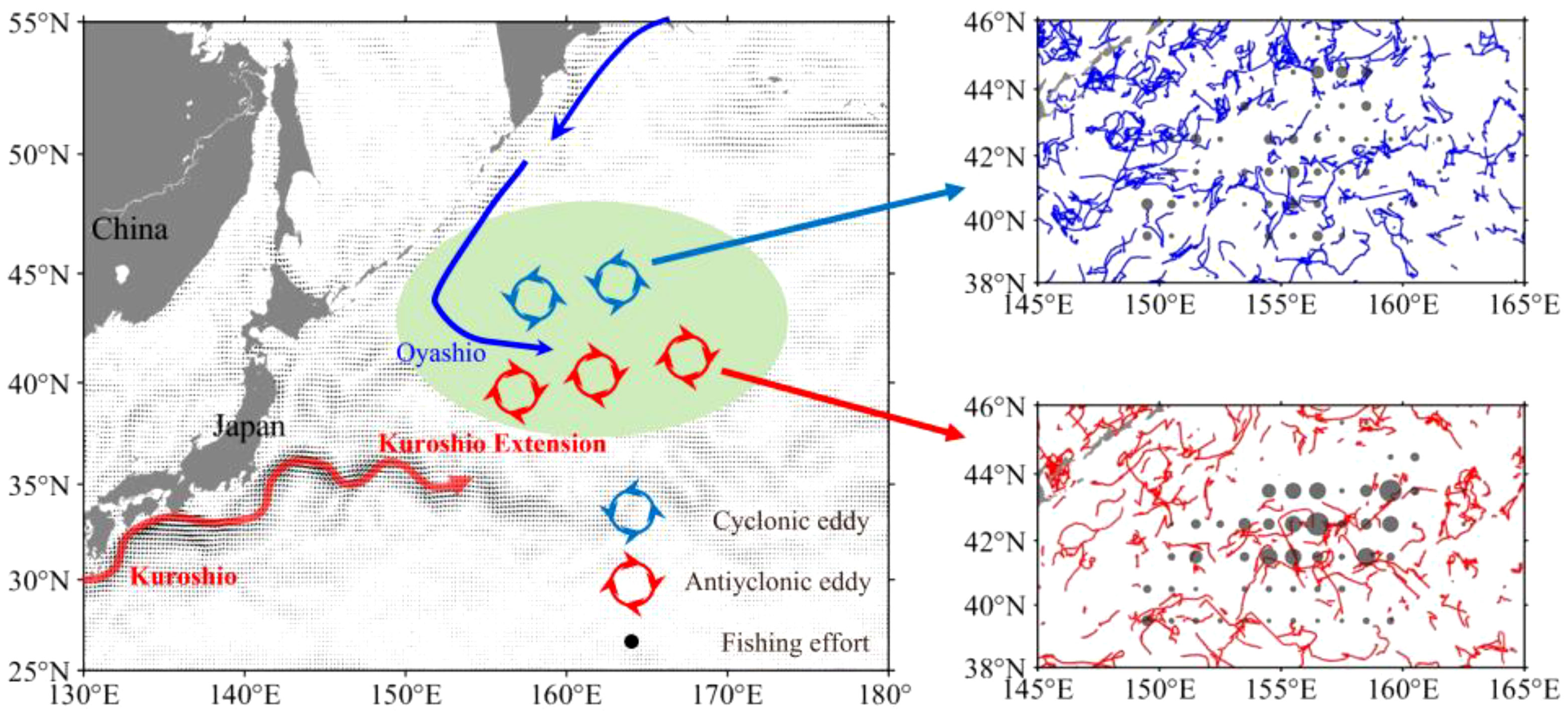
Figure 1 Schematic diagram of the Kuroshio, Oyashio and mesoscale eddies on the fishing ground of neon flying squid Ommastrephes bartramii in the Northwest Pacific Ocean and the average ocean current during the Kuroshio Extension unstable years in the background (left panel). Trajectory of cyclonic eddies (upper-right panel) and anticyclonic eddies (lower-right panel) overlaid with the fishing efforts inside the eddies in the fishing season during the unstable Kuroshio Extension years.

where catch and fishing efforts were the total catch and total fishing efforts, respectively. CPUE was used as an abundance index of O. bartramii stock.

2.2 Oceanographic data

According to Tian et al. (2020), multi-satellite merged altimeter data is more suitable for eddy tracking. Thus, this study uses an all-sat merged product (https://resources.marine.copernicus.eu/product-detail/SEALEVEL_GLO_PHY_L4_MY_008_047/INFORMATION). This up-to-date dataset includes up to four satellite missions and uses all available missions at any given time. The surface current velocity and Absolute Dynamic Topography (ADT) data used for the analysis of both KE dynamic state and mesoscale eddies were at a spatial and temporal resolution of 1/4° and daily.

Seawater temperatures at two different depths were obtained from the GLORYS12V1(https://resources.marine.copernicus.eu/product-detail/GLOBAL_MULTIYEAR_PHY_001_030/INFORMATION), which was sourced from the Copernicus Marine Environment Monitoring Service (CMEMS) global ocean eddy-resolving reanalysis with 1/12° (approximately 8 km) horizontal resolution and 50 standard vertical levels. Seawater temperature at two different layers was selected as Sea surface temperature (SST) and seawater temperature at 50-m depth (T_50m). Daily surface Chl-a concentration data were from Global Ocean Satellite Observation (Copernicus - GlobColour) (https://resources.marine.copernicus.eu/product-detail/OCEANCOLOUR_GLO_CHL_L4_REP_OBSERVATIONS_009_082/INFORMATION), and the reprocessed data were provided by CMEMS, which consisted of daily data interpolated and reprocessed from satellite observations and had a spatial resolution of 4 km. The Chl-a data were resampled to a uniform resolution with seawater temperature at 1/12°. All such ocean data were matched to the daily fishing locations using bilinear interpolation.

2.3 Methods

2.3.1 Kuroshio extension state analysis

In this study, the existence of a stable versus an unstable state of the KE system was emphasized, and the years from 2009 to 2018 were categorized as stable or unstable years. The main path of KE was defined as contour lines of SSH (Qiu and Chen, 2010), and we superimposed monthly KE paths separately to exhibit the two dynamic states of the KE.

2.3.2 Mesoscale eddy analysis

A state-of-the-art eddy detection algorithm based on physical parameters and geometrical properties is used to track the mesoscale eddies in this study (Le Vu et al., 2018). The eddies in the fishing ground were tracked daily, covering the spatial and temporal range of the fisheries data. Finally, eddies with a lifespan of fewer than 14 days were filtered due to their limited periods and impacts. Examples of the eddy tracking algorithm were showed in Figure S2 and Figure S3.

SST, T_50m, and Chl-a were analyzed to illustrate the eddy-induced oceanic changes on the fishing ground. A high-resolution grid with radial distance from the eddy center normalized by the eddy radius scale was built, covering the range of twice eddy radius ( ± 2R), while the radius of an individual eddy is defined as equal to the radius of a circle covering the same surface. The collocated values of oceanic factors were then referenced geographically to each eddy center and interpolated onto this grid, and then the grids were averaged over all eddies (Gaube et al., 2014). This normalization allows composites to be constructed from eddies of varying sizes on a common grid. To better represent the eddies that directly influence the O. bartramii fisheries, we counted the state of the eddies when there were fishing operations in the eddy that day.

2.3.3 Association between O. bartramii abundance and eddies

To investigate the effects of eddies on O. bartramii, the geospatial relationship between fisheries positions and eddies was analyzed. First, the distance from each fishing position to the geographically closest CE and AE was determined, respectively. A normalized relative distance was then used to illustrate the CPUE distribution with respect to the eddies. The relative distance was computed as follows:

$$Dx=\frac{Z_x}{R}$$

$$Dy=\frac{Z_y}{R}$$

where Z_x and Z_y were the zonal and meridional distance from the fishing position to the closest CE or AE center, R represented eddy radius and D_x and D_y were the normalized zonal and meridional relative distances, respectively. Additionally, a simple in-polygon algorithm was applied to accurately determine whether the fishing position was in the interior of an eddy, as the contours of eddies have been defined as approximate polygons.

2.3.4 Habitat suitability index model development and validation

In this study, a habitat suitability index (HSI) model was developed to evaluate the effects of the eddies on the O. bartramii habitat conditions. HSI was presented as an index on a scale of 0 – 1 as the combination or average of a suitable index (SIs) representing biophysical factors. SI was defined as the environmental preference of O. bartramii based on historical observation of abundance at different environmental values, ranging from 0 to 1 (Silva et al., 2016). Previous studies concluded that the favorable habitat ranges would be overestimated/underestimated only using one abundance indicator (Tian et al., 2009). Therefore, in this study, the SI value was quantified by averaging catch-based and effort-based SI values. Three factors, SST, T_50m and Chl-a, were selected to construct the HSI model with low collinearity been found. Each variable was divided into levels with intervals set to 1.0°C for SST and T_50m, and 0.1 mg/m³ for Chl-a, respectively. The catch-based SI value was calculated by the total catch of each class interval for each variable divided by the maximum catch of the classes for the variable, and the fishing effort-based SI was calculated by the same rule:

$${\text{SI}}_{i,k,\text{Catch}}=\frac{{\text{Catch}}_{i,k}}{{\text{Catch}}_{\text{max}}}$$

$${\text{SI}}_{i,k,\text{Effort}}=\frac{{\text{Effort}}_{i,k}}{{\text{Effort}}_{\text{max}}}$$

where Catch_i,k and Effort_i,k represent the sum of catch and fishing effort at class k for variable i; Catch_max and Effort_max represent the maximum of catch and fishing effort of the classes for variable i.

Then the catch-based and effort-based SI curves were fitted by an exponential parametric model, respectively:

$${\text{SI}}_{i,\text{Catch}}=\exp \left[a\times {\left({\text{variable}}_i-b\right)}^2\right]$$

$${\text{SI}}_{i,\text{Effort}}=\exp \left[a\times {\left({\text{variable}}_i-b\right)}^2\right]$$

where i represents the biophysical variable; a and b are the estimated model parameters, which were solved with a least square estimate to minimize the residuals between the observed and predicted SI values. The ultimate SI is calculated as follows:

$${\text{SI}}_i=\frac{1}{2}\left({\text{SI}}_{i,\text{Catch}}+{\text{SI}}_{i,\text{Effort}}\right)$$

The importance of model variables can be different. Thus, the HSI model was constructed based on a weighted arithmetic mean method (AMM). A total of 25 weighting scenarios were introduced to select the best combination of variable weights (Table S1). The weighted HSI model is calculated as follows:

$$\text{HSI}=\frac{1}{{\sum }_{i=1}^n{w}_i}\left({\text{SI}}_i\times w_i\right)$$

where SI_i is SI values for each variable i; w_i represents the weight of variable i; n is the number of variables included in the HSI model.

The weighted HSI model with the best performance was selected through a two-step test. First, the areas with HSI ≤ 0.2, with 0.2< HSI< 0.6, and with HSI ≥ 0.6 was defined as poor, common, and suitable habitat, respectively, for O. bartramii (Yu et al., 2015). For the optimal weighting scenario, the percentage of catch and fishing effort accounting for the total catches and fishing efforts in suitable habitats should be the highest and in poor habitats be the lowest, and with an increasing HSI, the CPUE also increased (Yu et al., 2019). After that, model performance was also evaluated by examining the linear relationship between the CPUE and HSI values.

2.3.5 Evaluation of the influences of cyclonic and anticyclonic eddy

We further explored the potential mechanisms of how mesoscale eddies affected the O. bartramii distribution. Based on the HSI model, how eddies modulated the distribution pattern of O. bartramii habitats was illustrated. The distribution pattern of SI value for each environmental factor and the integrated HSI value in the range of twofold eddy radius ( ± 2R) were shown in the same way as described above in 2.3.2. The SI and HSI values inside CEs and AEs were further quantitatively compared. As the areas with SI≥0.6 and HSI ≥0.6 were defined as suitable one-factor environmental conditions and suitable habitats, referring to the areas with high O. bartramii abundance, the proportion of these suitable areas within the CE and AE areas were also quantified.

3 Results

3.1 KE dynamic state

The annual dynamic state of the KE was shown by the 90-cm ADT contours representing the KE main path in the region between 30°-40°N and 140°-160°E (Figure S1). Two different dynamic states of the KE were exhibited: during 2009, 2016, and 2017, the KE underwent an unstable state, and it showed a more convoluted path with a large meridional fluctuation; while during the other years, the KE was at a relatively stable path with two quasi-stationary meanders. The monthly KE paths and the average EKE in the fishing season (July to November) during the stable and unstable years were shown in Figure 2. During the stable KE years, high EKE occurred along the main path of the KE, while in the unstable KE years, high EKE extended more widely due to a strongly fluctuating KE path.

FIGURE 2

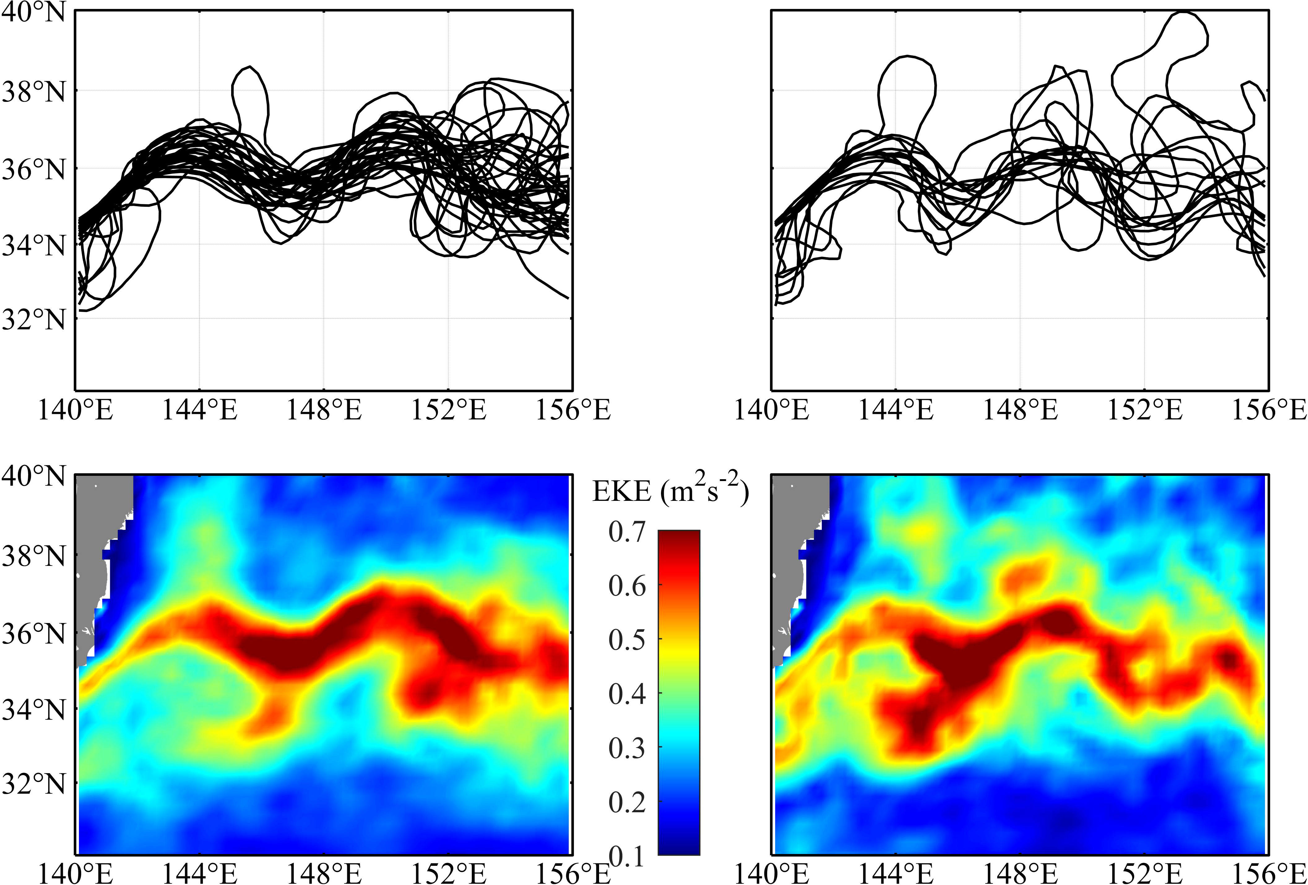
Figure 2 The monthly Kuroshio Extension (KE) path defined by the longest contour of 90 cm absolute dynamic topography (ADT) from July to November during the stable KE years (upper-left panel) and unstable years (upper-right panel). Average eddy kinetic energy (EKE) from July to November during the stable KE years (lower-left panel) and unstable years (lower-right panel).

3.2 Variations in O. bartramii catch and CPUE in relation to the KE dynamic state-related eddies changes

The variation of the abundance and distribution of O. bartramii with respect to eddies was shown, and a dramatic difference in O. bartramii CPUE between CEs and AEs was only found during the unstable KE years (Figure 3). The distribution pattern of CPUE in and around the two types of eddies was quite different. Widespread high CPUE was observed in the AE interior (Figure 3 lower-left panel), while it was sparse and much lower in the CE (Figure 3 upper-left panel). The total catch in AEs was approximately 11.5 times that of CEs (Figure 3 upper-right panel) and the median CPUE in AEs was about 70% higher than CEs (Figure 3 lower-right panel).

FIGURE 3

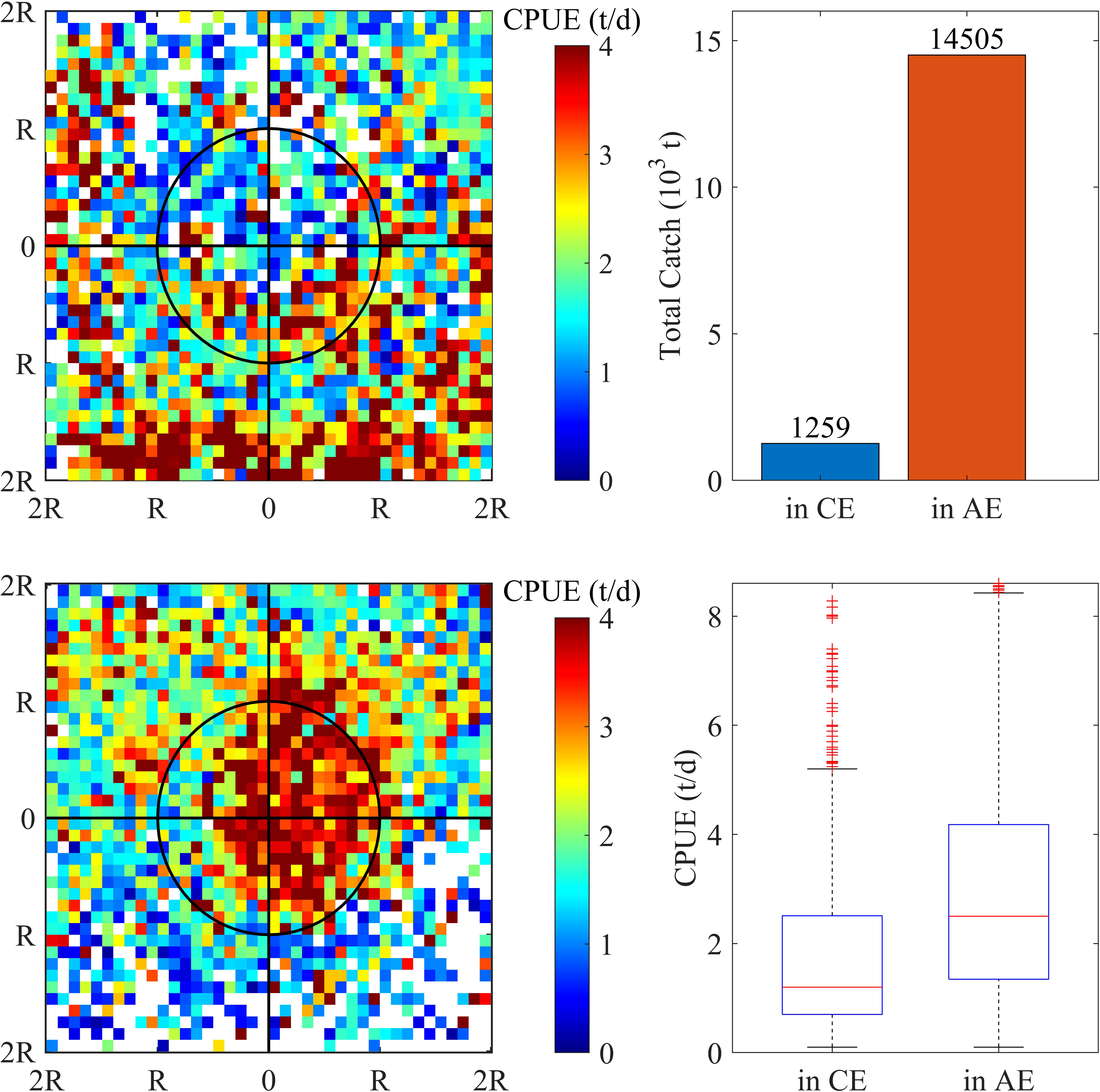
Figure 3 During the unstable Kuroshio Extension years, the distribution of O. bartramii CPUE (catch per unit effort) in the area of twofold radius ( ± 2R) of the cyclonic (upper-left panel) and anticyclonic eddies (lower-left panel). The distance was normalized by the radius of each individual eddy. Total catch (upper-right panel) and CPUE (upper-right panel) in the interior of cyclonic and anticyclonic eddies.

3.3 Eddy detection analysis and eddy-induced environmental changes

The trajectory of CEs and AEs and the distribution of fishing effort in the eddies during the KE unstable years were shown in Figure 1. Figure 4 showed the distribution pattern of the SST, T_50m, and Chl-a in and around the eddies. There was no significant difference in SST in the core of the two different types of eddies, but the pattern of temperature distribution differed because of the advection driven by the opposite rotational directions. The vertical flows, generally, upwelling in the CE and downwelling in the AE, caused significantly different distribution patterns of T_50m and Chl-a. The median difference in T_50m was higher than 2°C. Chl-a significantly increased and decreased in CEs and ACs, respectively, compared with the outside of the eddies.

FIGURE 4

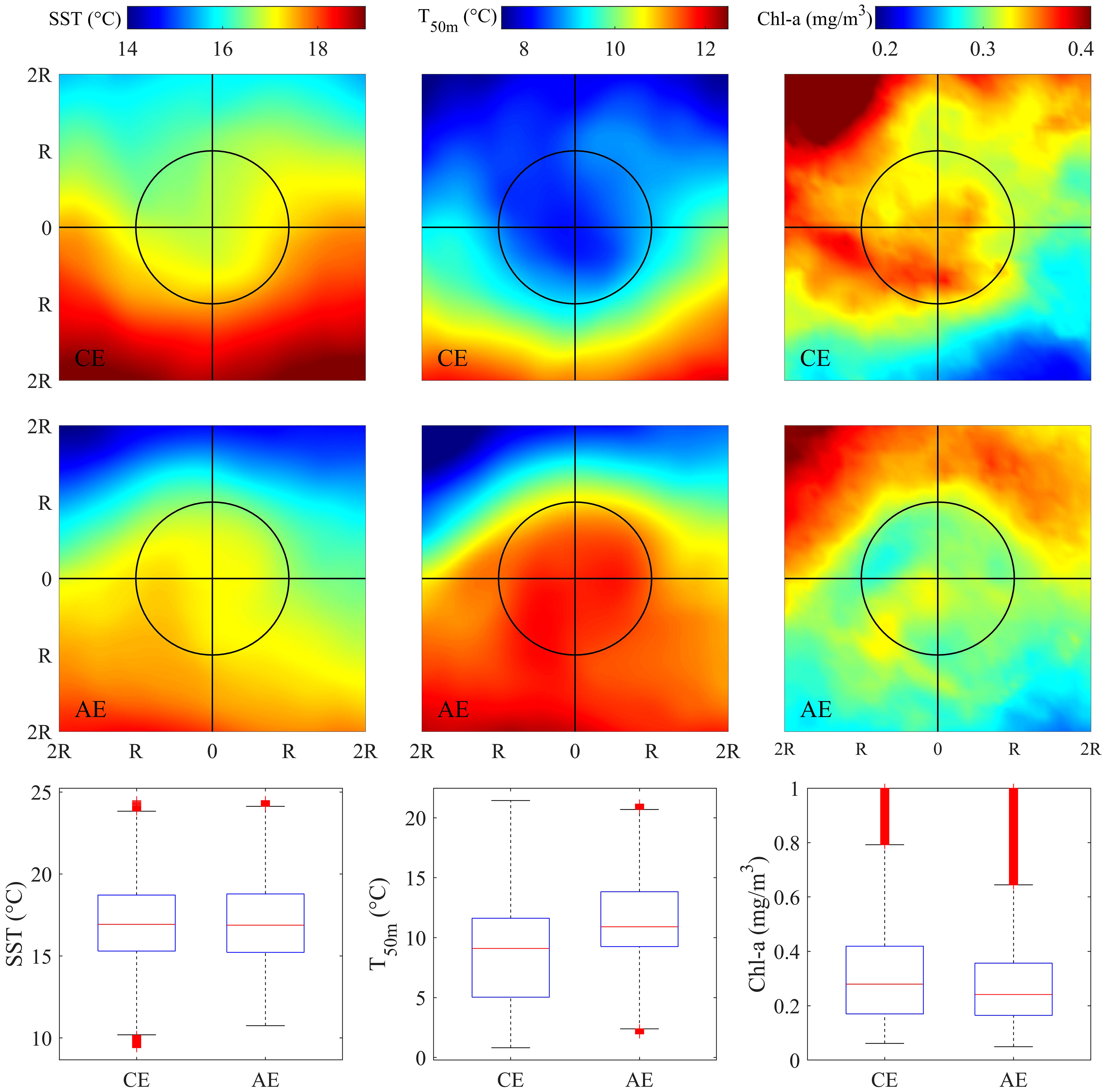
Figure 4 Spatial pattern of averaged sea surface temperature (SST), seawater temperature at depth of 50m (T_50m) and sea surface chlorophyll-a concentration (Chl-a) in the area of twofold radius ( ± 2R) of the cyclonic (upper panel) and anticyclonic eddies (middle panel) on the fishing ground. Boxplot of SST, T_50m and Chl-a in the interior of cyclonic and anticyclonic eddies during the unstable Kuroshio Extension years (bottom panel).

3.4 HSI model

The fitted curve, model, and statistical parameters of the monthly SI model established for each factor (SST, T_50m, and Chl-a) were shown in Figure S4 and Table S2. All the SI models were statistically significant (P<0.001) and with high correlation (R²>0.8).

To select the best weighting scenario, we first compared the frequency of the catch in each HSI class interval under different weighing scenarios (Table S3). The HSI model based on weighting scenarios case 10, with weights of SST, T_50m, and Chl-a being 0.25, 0.5, and 0.25, was considered to be the optimal model as the frequency of catch in suitable habitats was the highest and in poor habitats was the lowest, and CPUE increased with the higher HSI. Linear regression analysis showed that 70% of the variance in mean CPUE was explained by the HSI model (R² = 0.7) (Figure S5). Thus, the HSI model under weighting scenario case 10 was chosen as the optimal model.

3.5 Eddy-induced changes in distribution pattern of suitable habitats

The spatial pattern of the SI value for SST, T_50m and Chl-a derived from the composite averages constructed from eddies were shown in Figures 5A, B. Compared to CEs, high SIs were observed in the interior of AEs, with a strong gradient showing near the eddy periphery. The relative difference of each SI in the interior of CEs and AEs, as well as the proportion of suitable SI (SI ≥ 0.6) to the eddy area, were illustrated and quantified (Figures 5C, D and Table S4). For each environmental factor, the SI and the proportion of the suitable SI to the eddy area were higher in AEs than CEs, especially for T_50m and Chl-a. Mean SI and the proportion of suitable SI for T_50m were higher in AE than CE by 12.25% and 30.47%, and 20.30% and 23.52% for Chl-a. The difference was smaller but still persistent for SST, with mean SI and the proportion of suitable SI being higher by 6.08% and 13.85%.

FIGURE 5

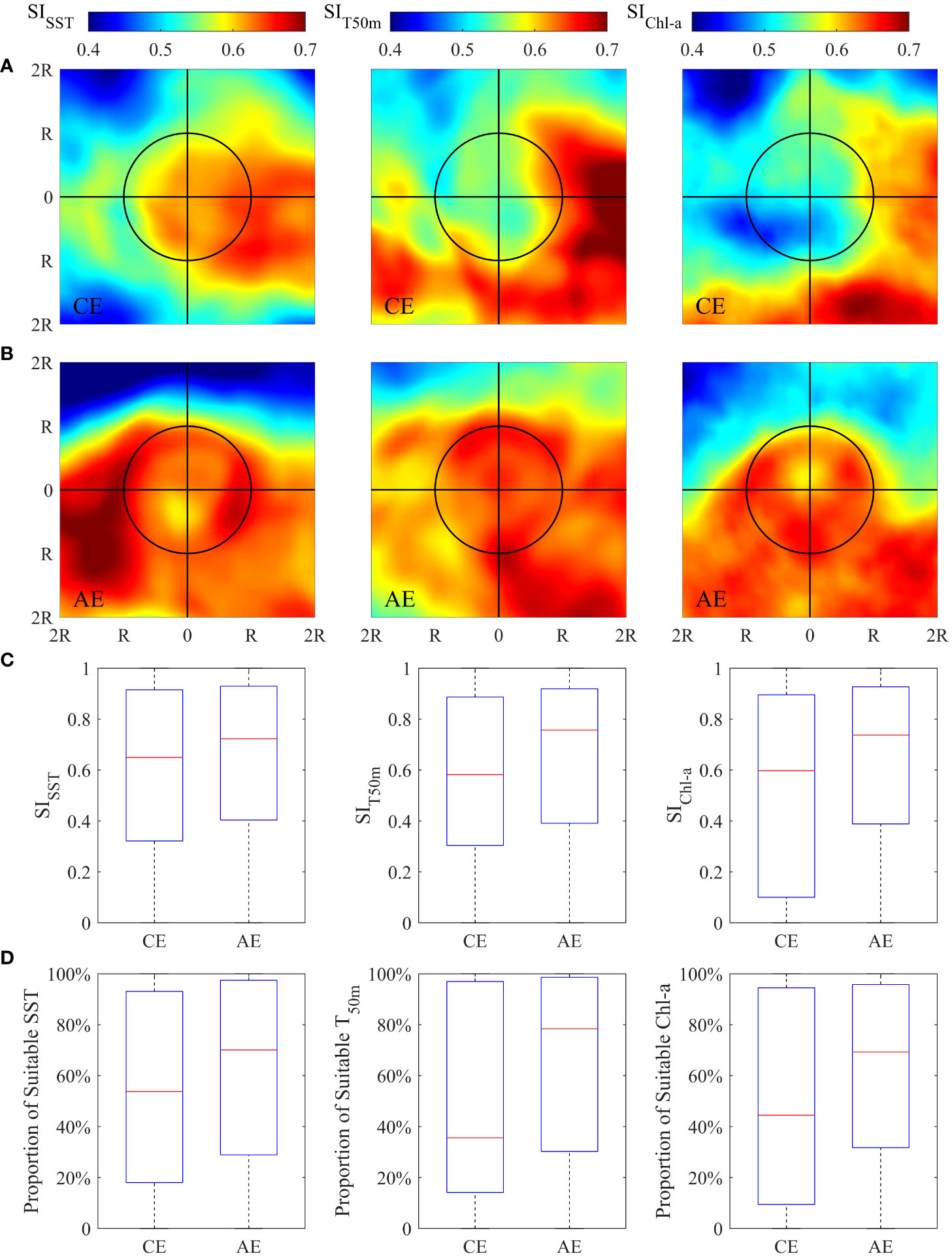
Figure 5 Spatial pattern of averaged suitability index for sea surface temperature (SST), seawater temperature at depth of 50m (T_50m) and sea surface chlorophyll-a concentration (Chl-a), respectively, in the area of twofold radius ( ± 2R) of the cyclonic (panel A) and anticyclonic eddies (panel B) on the fishing ground. Boxplot of SI_SST, SI_T50m and SI_Chl-a in the interior of cyclonic and anticyclonic eddies (panel C). Boxplot of the proportion of suitable SST, T_50m and Chl-a (SI≥0.6) to the area of cyclonic and anticyclonic eddies (panel D).

The distribution of the integrated HSI in and around the eddies is shown in Figure 6. Significant differences in squid habitat quality were found within AE and CE. It can be inferred that AEs tended to be capable of forming favorable habitats for O. bartramii according to the observed higher HSI. Average HSI within AE was higher than CE by 12.47% and the proportion of suitable HSI to the eddy area of AE was higher than CE by 43.57% (Table S4).

FIGURE 6

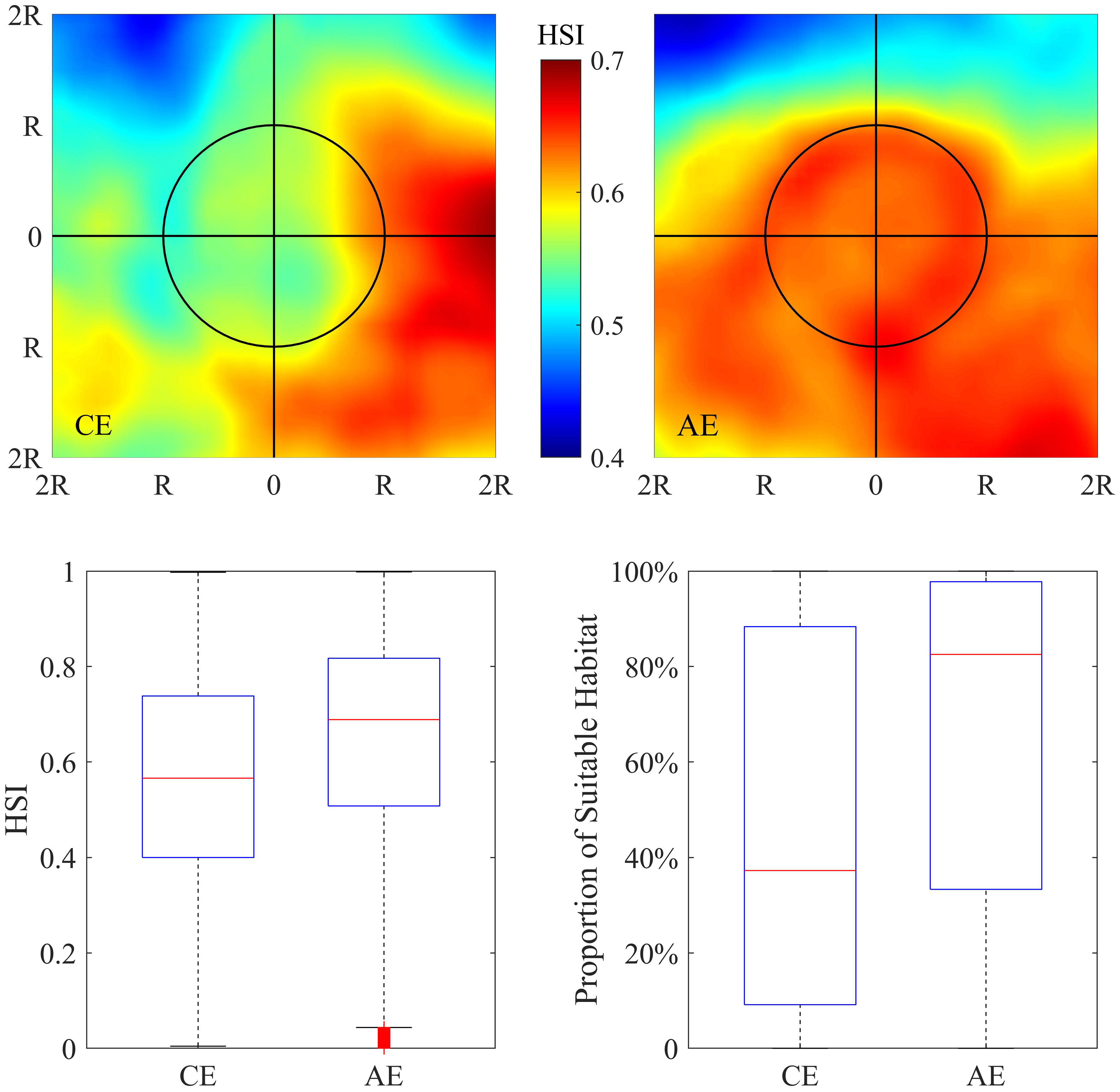
Figure 6 Pattern of averaged habitat suitability index (HSI) in the area of twofold radius ( ± 2R) of the cyclonic (upper-left panel) and anticyclonic eddies (upper-right panel). Boxplot of HSI in the interior of cyclonic and anticyclonic eddies (lower-left panel). Boxplot of the proportion of suitable habitats (HSI≥0.6) to the area of cyclonic and anticyclonic eddies (lower-right panel).

4 Discussion

In this study, the impacts of mesoscale eddies on the abundance and distribution of O. bartramii were evaluated in the Northwest Pacific Ocean. Cold-core CEs and warm-core AEs were found to have different impacts on O. bartramii population. A significantly higher abundance of O. bartramii was found in AEs than in CEs during KE unstable years, with a much higher catch and 70% higher CPUE (Figure 3). Based on a weighted AMM based HSI model with crucial ecological factors considered, the eddy-induced O. bartramii habitat distribution patterns were shown (Figure 6). The pattern of habitat explained the variation of O. bartramii distribution in and around the eddies.

Eddies have long been recognized as important oceanic features forming good fishing grounds of O. bartramii. In previous studies, the main mechanisms by which the eddy activities influence the O. bartramii distribution were generally considered to be related to the foraging conditions. The enhanced primary production stimulated by nutrient supply from upwelling occurring at the center of CEs and the edge of AEs (Chen et al., 2010b; Yu et al., 2016), and the aggregation of prey induced by the convergent flow at the center of AEs (Alabia et al., 2015), were believed to be the main reasons that the eddy activities attracted O. bartramii. However, little attention has been paid to the effects of eddies on the thermal adaptation of O. bartramii, especially based on the general understanding that warm-core AEs are oligotrophic (Gaube et al., 2014). And although seawater temperature, either at the surface or subsurface, has been recognized as a crucial factor affecting the distribution of O. bartramii, the link between this factor and the mesoscale eddies has been neglected. In this study, specific distribution patterns of biophysical factors indicating the thermal and nutrient conditions and their corresponding SIs in and around the eddies were shown (Figures 4 and 5). The effects of the factors were found of varying importance, with T_50m being considered the most important. It is suggested that the elevated T_50m in AEs producing an expanded suitable SI range was the main cause of the high O. bartramii abundance in the warm-core AEs. As for CEs, though the observed high Chl-a indicates high productivity conditions, the unfavorable thermal conditions prevented them from being very suitable habitats for O. bartramii.

O. bartramii is a pelagic warm water species. SST has long been considered as a crucial or dominant factor affecting the distribution of O. bartramii (Tian et al., 2009; Yu et al., 2019), in addition, increasing attention has also been paid to the role of the subsurface temperature (Alabia et al., 2016; Wang et al., 2022). In this study, T_50m was selected to characterize subsurface temperature. O. bartramii performs a typical diel vertical migration pattern (Murata and Nakamura, 1998), and they are fished by consistent specific squid jigging operation at about 50-m depth when floating to forage at nighttime. Previous studies have highlighted the role of the temperature vertical structure from the surface to 50-m depth in forming fishing grounds for O. bartramii (Chen et al., 2014). A recent study investigated the effects of subsurface temperature on O. bartramii in the Northwest Pacific Ocean and found that O. bartramii prefer relatively warm water at 30-m depth ranging from 11 – 18°C(Wang et al., 2022). The preference of O. bartramii to subsurface warm water at such depth is probably because it can meet the thermal needs of this ectothermic species during predation.

The HSI model has been widely used in fisheries, ecological impact assessments, and ecological restoration studies. It has been successfully applied to the evaluation and prediction of habitat changes of O. bartramii (Igarashi et al., 2018; Yu et al., 2020). A reliable proxy of species abundance and distribution is crucial to the model. Previous studies concluded that using a CPUE-based HSI model might overestimate the favorable habitat ranges and underestimate the variations in habitat spatial distribution (Tian et al., 2009). In this study, both abundance and presence indicators were taken into consideration in the model development by combining catch and fishing efforts into the aggregation of the HSI model. Three biophysical factors proven to have significant impacts on the O. bartramii habitat, SST, T_50m, and Chl-a, were considered in the model. In addition to the temperature variables mentioned above, Chl-a is another factor often used in the habitat assessment of O. bartramii, which indicated the primary production and food availability (Yu et al., 2019). As O. bartramii does not feed on phytoplankton directly, the effect of Chl-a on O. bartramii population should be indirect, yet a significant association between Chl-a and squid distribution existed (Table S2). By comparing the performance of the weighted AMM-based HSI model under different empirical weighting scenarios (Table S1), the varying importance of factors was shown, and the optimal weight combination was considered to be 0.25, 0.5, and 0.25 for SST, T_50m, and Chl-a, respectively (Table S3). Finally, the model showed excellent prediction performance (Figure S4).

Since the HSI model was built using all the fisheries data in this study, it is based on the assumption that the response of O. bartramii to the biophysical factors was spatially consistent. This means that for each environmental factor included in the model, we assumed that its effect was the same whether it was inside or outside the eddies. The distribution of these variables in the ocean is not completely independent of each other while is appeared to show specific combinations in different regions, and these variables affected the distribution of O. bartramii together. As for two types of eddies, it is generally a combination of low T_50m and high Chl-a in CEs while a combination of high T_50m and low Chl-a in AEs (Figure 4). Although sometimes the effects of mixing in AEs may cause an increase in Chl-a, a low Chl characteristic was still evident from the long-term average. The especially high O. bartramii abundance found in AEs indicated its preference for high T_50m and a relatively suitable Chl-a range or some other properties associated with such conditions. Using an abundance proxy based on the frequency of fishing effort and catch as well as integrating each individual SI in model construction, the preference of O. bartramii for such a combination was evaluated.

An interannual variation of O. bartramii abundance inside warm-core AEs possibly related to the KE dynamic states was found. During the stable KE state, the abundance of O. bartramii was also higher in AEs than CEs. The total catch in AEs was several times that of CEs, while the difference in CPUE was smaller compared to the unstable KE state (Figure S6). Revealing the mechanisms of this interannual variation was beyond the scope of this paper, but some speculations have been proposed. Previous studies have observed increasing regional chlorophyll concentration in the Northwest Pacific during the unstable KE years (Lin et al., 2014). The distribution of fishing effort in AEs and the spatial patterns of Chl-a in AEs in the region with dense effort distribution were shown during the two KE dynamic states (Figure 7). Higher Chl-a in AEs were observed during the unstable KE years, which might be attributed to changes in the chlorophyll background field due to specific ocean circulation associated with an unstable KE. The combination of the suitable subsurface warm water and the favorable nutrient conditions in the unstable KE background could be the main drivers for yielding particularly high O. bartramii abundance in the warm eddies.

FIGURE 7

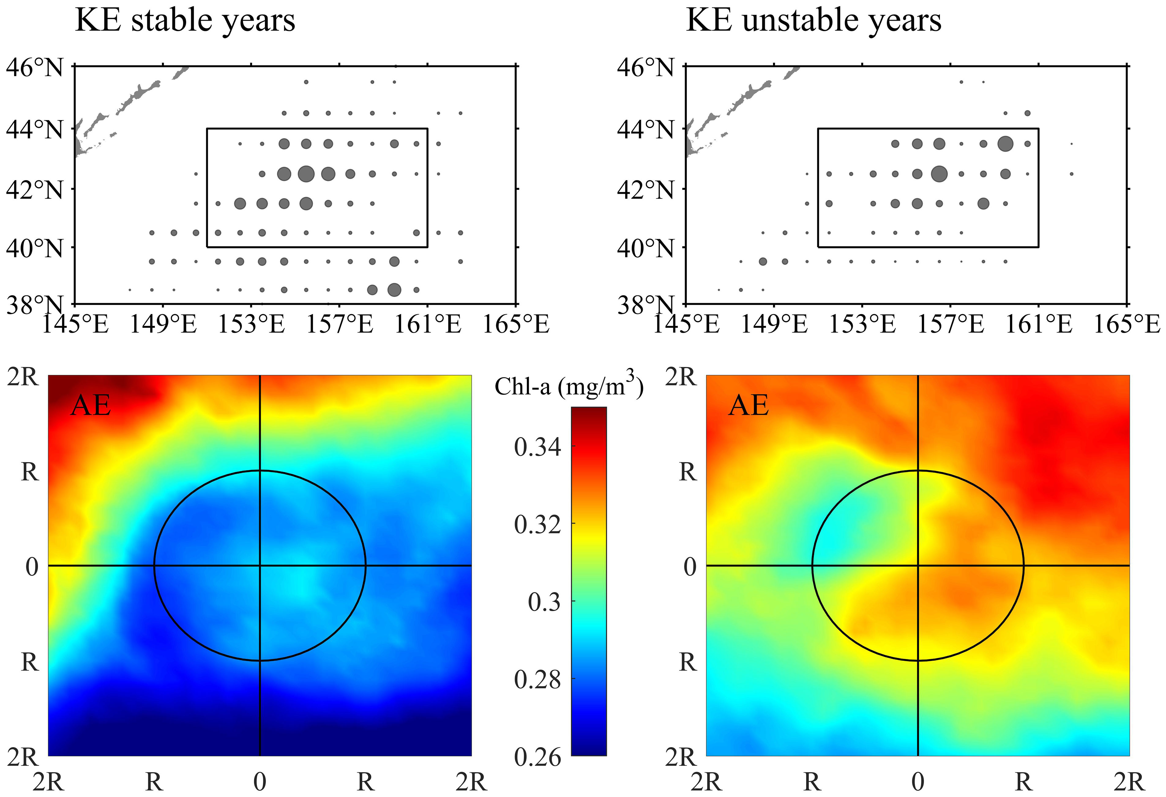
Figure 7 The distribution of fishing effort in anticyclonic eddies (AE) during the stable Kuroshio Extension (KE) years (upper-left panel) and unstable years (upper-right panel) and spatial pattern of Chl-a in the area of twofold radius ( ± 2R) of AEs in region bounded by 40°-44°N and 151°-161°E (denoted in the upper panels) during the stable Kuroshio Extension (KE) years (lower-left panel) and unstable years (lower-right panel).

In summary, warm-core AEs were found to yield high O. bartramii abundance mainly because of the favorable subsurface thermal condition. The impacts of the eddies on the O. bartramii population, especially of AEs, might change with the interannual KE variability, although its mechanism has not been clearly revealed yet. Other interannual or decadal climate changes, such as the El Niño Southern Oscillation, which significantly affected the biophysical environments in the Northwest Pacific Ocean, may also play a role in influencing the eddy variations, and as a result, affecting squid species, necessitating further research.

Data availability statement

The original contributions presented in the study are included in the article/Supplementary Material. Further inquiries can be directed to the corresponding author.

Author contributions

WY, YZ, and XC conceptualized the study. WY, YZ and MZ designed the methodology and provided the software analyzed the data for the study. YZ and WY wrote the original draft. WY, XC and CZ involved in the funding acquisition. All authors contributed to the article and approved the submitted version. All authors have given approval to the final version of the manuscript.

Funding

This study was financially supported by the National Natural Science Foundation of China (41906073, 42106090), the project of Shanghai talent development funding (2021078), the National Key R&D Program of China (2019YFD0901405), the Natural Science Foundation of Shanghai (19ZR1423000), and the open fund of State Key Laboratory of Satellite Ocean Environment Dynamics, Second Institute of Oceanography (QNHX2232).

Conflict of interest

The authors declare that the research was conducted in the absence of any commercial or financial relationships that could be construed as a potential conflict of interest.

Publisher’s note

All claims expressed in this article are solely those of the authors and do not necessarily represent those of their affiliated organizations, or those of the publisher, the editors and the reviewers. Any product that may be evaluated in this article, or claim that may be made by its manufacturer, is not guaranteed or endorsed by the publisher.

Supplementary material

The Supplementary Material for this article can be found online at: https://www.frontiersin.org/articles/10.3389/fmars.2022.862273/full#supplementary-material

References

Alabia I. D., Saitoh S. I., Igarashi H., Ishikawa Y., Usui N., Kamachi M., et al. (2016). Ensemble squid habitat model using three-dimensional ocean data. ICES J. Mar. Sci. 73 (7), 1863–1874. doi: 10.1093/icesjms/fsw075

CrossRef Full Text | Google Scholar

Alabia I. D., Saitoh S. I., Mugo R., Igarashi H., Ishikawa Y., Usui N., et al. (2015). Identifying pelagic habitat hotspots of neon flying squid in the temperate waters of the central north pacific. PLoS One 10 (11), e0142885. doi: 10.1371/journal.pone.0142885

PubMed Abstract | CrossRef Full Text | Google Scholar

Bower J. R., Ichii T. (2005). The red flying squid (Ommastrephes bartramii): A review of recent research and the fishery in Japan. Fish. Res. 76 (1), 39–55. doi: 10.1016/j.fishres.2005.05.009

CrossRef Full Text | Google Scholar

Braun C. D., Gaube P., Sinclair-Taylor T. H., Skomal G. B., Thorrold S. R. (2019). Mesoscale eddies release pelagic sharks from thermal constraints to foraging in the ocean twilight zone. P. Nat. Acad. Sci. U.S.A. 116 (35), 17187–17192. doi: 10.1073/pnas.1903067116

CrossRef Full Text | Google Scholar

Chelton D. B., Gaube P., Schlax M. G., Early J. J., Samelson R. M. (2011b). The influence of nonlinear mesoscale eddies on near-surface oceanic chlorophyll. Science. 334 (6054), 328–332. doi: 10.1126/science.1208897

PubMed Abstract | CrossRef Full Text | Google Scholar

Chelton D. B., Schlax M. G., Samelson R. M. (2011a). Global observations of nonlinear mesoscale eddies. Prog. Oceanogr. 91 (2), 167–216. doi: 10.1016/j.pocean.2011.01.002

CrossRef Full Text | Google Scholar

Chen X. J. (1995). An approach to the relationship between the squid fishing ground and water temperature in the northwest pacific. J. Shanghai Fisheries University. 4, 181–185.

Google Scholar

Chen X. J., Cao J., Chen Y., Liu B. L., Tian S. Q. (2012). Effect of the kuroshio on the spatial distribution of the red flying squid Ommastrephes bartramii in the Northwest pacific ocean. B. Mar. Sci. 88 (1), 63–71. doi: 10.5343/bms.2010.1098

CrossRef Full Text | Google Scholar

Chen X. J., Cao J., Tian S. Q., Liu B. L., Li S. L. (2010a). Effect of inter-annual change in sea surface water temperature and kuroshio on fishing ground of squid Ommastrephes bartramii in the Northwest pacific. J. Dalian Fisheries University. 25 (2), 119–126. doi: 10.3969/j.issn.1000-9957.2010.02.005

CrossRef Full Text | Google Scholar

Chen X. J., Chen Y., Tian S. Q., Liu B. L., Qian W. G. (2008b). An assessment of the west winter-spring cohort of neon flying squid (Ommastrephes bartramii) in the Northwest pacific ocean. Fish. Res. 92 (2-3), 221–230. doi: 10.1016/j.fishres.2008.01.011

CrossRef Full Text | Google Scholar

Chen X. J., Liu B. L., Chen Y. (2008a). A review of the development of Chinese distant-water squid jigging fisheries. Fish. Res. 89 (3), 211–221. doi: 10.1016/j.fishres.2007.10.012

CrossRef Full Text | Google Scholar

Chen X. J., Tian S. Q., Chen Y., Liu B. L. (2010b). A modeling approach to identify optimal habitat and suitable fishing grounds for neon flying squid (Ommastrephes bartramii) in the Northwest pacific ocean. Fish. Bull. 108 (1), 14.

Google Scholar

Chen X. J., Tian S. Q., Guan W. J. (2014). Variations of oceanic fronts and their influence on the fishing grounds of Ommastrephes bartramii in the Northwest pacific. Acta Oceanol. Sin. 33 (4), 45–54. doi: 10.1007/s13131-014-0452-3

CrossRef Full Text | Google Scholar

Chen X. J., Tian S. Q., Liu B. L., Chen Y. (2011). Modeling a habitat suitability index for the eastern fall cohort of Ommastrephes bartramii in the central north pacific ocean. Chin. J. Oceanol. Limn. 29 (3), 493–504. doi: 10.1007/s00343-011-0058-y

CrossRef Full Text | Google Scholar

Gaube P., Braun C. D., Lawson G. L., McGillicuddy D. J., Della Penna A., Skomal G. B., et al. (2018). Mesoscale eddies influence the movements of mature female white sharks in the gulf stream and Sargasso Sea. Sci. Rep. 8, 7363. doi: 10.1038/s41598-018-25565-8

PubMed Abstract | CrossRef Full Text | Google Scholar

Gaube P., McGillicuddy D. J., Chelton D. B., Behrenfeld M. J., Strutton P. G. (2014). Regional variations in the influence of mesoscale eddies on near-surface chlorophyll. J. Geophys. Res-Oceans. 119 (12), 8195–8220. doi: 10.1002/2014JC010111

CrossRef Full Text | Google Scholar

Godø O. R., Samuelsen A., Macaulay G. J., Patel R., Hjøllo S. S., Horne J., et al. (2012). Mesoscale eddies are oases for higher trophic marine life. PLoS One 7 (1), e30161. doi: 10.1371/journal.pone.0030161

PubMed Abstract | CrossRef Full Text | Google Scholar

Gómez G. S. D., Nagai T., Yokawa K. (2020). Mesoscale warm-core eddies drive interannual modulations of swordfish catch in the kuroshio extension system. Front. Mar. Sci. 7. doi: 10.3389/fmars.2020.00680

CrossRef Full Text | Google Scholar

Hsu A. C., Boustany A. M., Roberts J. J., Chang J. H., Halpin P. N. (2015). Tuna and swordfish catch in the US northwest Atlantic longline fishery in relation to mesoscale eddies. Fish. Oceanogr. 24 (6), 508–520. doi: 10.1111/fog.12125

PubMed Abstract | CrossRef Full Text | Google Scholar

Igarashi H., Saitoh S. I., Ishikawa Y., Kamachi M., Usui N., Sakai M., et al. (2018). Identifying potential habitat distribution of the neon flying squid (Ommastrephes bartramii) off the eastern coast of Japan in winter. Fish. Oceanogr. 27 (1), 16–27. doi: 10.1111/fog.12230

CrossRef Full Text | Google Scholar

Ishak N. H. A., Tadokoro K., Okazaki Y., Kakehi S., Suyama S., Takahashi K. (2020). Distribution, biomass, and species composition of salps and doliolids in the oyashio-kuroshio transitional region: potential impact of massive bloom on the pelagic food web. J. Oceanogr. 76 (5), 351–363. doi: 10.1007/s10872-020-00549-3

CrossRef Full Text | Google Scholar

Jayne S. R., Hogg N. G., Waterman S. N., Rainville L., Donohue K. A., Watts D. R., et al. (2009). The kuroshio extension and its recirculation gyres. Deep-Sea. Res. Pt I. 56 (12), 2088–2099. doi: 10.1016/j.dsr.2009.08.006

CrossRef Full Text | Google Scholar

Le Vu B., Stegner A., Arsouze T. (2018). Angular momentum eddy detection and tracking algorithm (AMEDA) and its application to coastal eddy formation. J. Atmos. Ocean. Tech. 35 (4), 739–762. doi: 10.1175/JTECH-D-17-0010.1

CrossRef Full Text | Google Scholar

Lin P. F., Chai F., Xue H. J., Xiu P. (2014). Modulation of decadal oscillation on surface chlorophyll in the kuroshio extension. J. Geophys. Res-Oceans. 119 (1), 187–199. doi: 10.1002/2013JC009359

CrossRef Full Text | Google Scholar

McGillicuddy D. J. Jr. (2016). Mechanisms of physical-biological-biogeochemical interaction at the oceanic mesoscale. Annu. Rev. Mar. Sci. 8, 125–159. doi: 10.1146/annurev-marine-010814-015606

CrossRef Full Text | Google Scholar

Murata M. (1993). Life history and biological information on flying squid (Ommastrephes bartramii) in the north pacific ocean. Bull. Int. Nat. North Pacific Commun. 53, 147–182.

Google Scholar

Murata M., Nakamura Y. (1998). “Seasonal migration and diel vertical migration of the neon flying squid, ommastrephes bartramii, in the north pacific,” in Proceedings of the contributed papers to international symposium on Large pelagic squids (Tokyo: Japan: Marine Fishery Resource Research center), 13–30.

Google Scholar

Ohshimo S., Hiraoka Y., Sato T., Nakatsuka S. (2018). Feeding habits of bigeye tuna (Thunnus obesus) in the north pacific from 2011 to 2013. Mar. Freshwater. Res. 69 (4), 585–606. doi: 10.1071/MF17058

CrossRef Full Text | Google Scholar

Polovina J., Uchida I., Balazs G., Howell E. A., Parker D., Dutton P. (2006). The kuroshio extension bifurcation region: A pelagic hotspot for juvenile loggerhead sea turtles. Deep-Sea. Res. Pt Ii. 53 (3-4), 326–339. doi: 10.1016/j.dsr2.2006.01.006

CrossRef Full Text | Google Scholar

Qiu B., Chen S. M. (2005). Variability of the kuroshio extension jet, recirculation gyre, and mesoscale eddies on decadal time scales. J. Phys. Oceanogr. 35 (11), 2090–2103. doi: 10.1175/JPO2807.1

CrossRef Full Text | Google Scholar

Qiu B., Chen S. M. (2010). Eddy-mean flow interaction in the decadally modulating kuroshio extension system. Deep-Sea. Res. Pt Ii. 57 (13-14), 1098–1110. doi: 10.1016/j.dsr2.2008.11.036

CrossRef Full Text | Google Scholar

Schmid M. S., Cowen R. K., Robinson K., Luo J. Y., Briseno-Avena C., Sponaugle S. (2020). Prey and predator overlap at the edge of a mesoscale eddy: Fine-scale, in-situ distributions to inform our understanding of oceanographic processes. Sci. Rep. 10, (1). doi: 10.1038/s41598-020-57879-x

PubMed Abstract | CrossRef Full Text | Google Scholar

Shao Q. Q., Ma W. W., Chen Z. Q., You Z. M., Wang W. Y. (2005). Relationship between kuroshio meander pattern and Ommastrephes bartramii CPUE in northwest pacific ocean. Oceanologia Limnologia Sinica 36 (2), 111–122. doi: 10.3321/j.issn:0029-814X.2005.02.003

CrossRef Full Text | Google Scholar

Silva C., Andrade I., Yáñez E., Hormazabal S., Barbieri M.Á., Aranis and A., et al. (2016). Predicting habitat suitability and geographic distribution of anchovy (Engraulis ringens) due to climate change in the coastal areas off Chile. Prog. Oceanogr. 146, 159–174. doi: 10.1016/j.pocean.2016.06.006

CrossRef Full Text | Google Scholar

Tian S. Q., Chen X. J., Chen Y., Xu L. X., Dai X. J. (2009). Evaluating habitat suitability indices derived from CPUE and fishing effort data for ommatrephes bratramii in the northwestern pacific ocean. Fish. Res. 95 (2-3), 181–188. doi: 10.1016/j.fishres.2008.08.012

CrossRef Full Text | Google Scholar

Tian F. L., Wu D., Yuan L. M., Chen G. (2020). Impacts of the efficiencies of identification and tracking algorithms on the statistical properties of global mesoscale eddies using merged altimeter data.Int. J. Remote. Sens. 41 (8), 2835–2860. doi: 10.1080/01431161.2019.1694724

CrossRef Full Text | Google Scholar

Waite A. M., Raes E., Beckley L. E., Thompson P. A., Griffin D., Saunders M., et al. (2019). Production and ecosystem structure in cold-core vs. warm-core eddies: Implications zooplankton isoscape rock lobster larvae. Limnol. Oceanogr. 64 (6), 2405–2423. doi: 10.1002/lno.11192

CrossRef Full Text | Google Scholar

Wang J. T., Cheng Y. Q., Lu H. J., Chen X. J., Lin L., Zhang J. B. (2022). Water temperature at different depths affects the distribution of neon flying squid (Ommastrephes bartramii) in the Northwest pacific ocean. Front. Mar. Sci. 8. doi: 10.3389/fmars.2021.741620

PubMed Abstract | CrossRef Full Text | Google Scholar

Watanabe H., Kubodera T., Ichii T., Kawahara S. (2004). Feeding habits of neon flying squid Ommastrephes bartramii in the transitional region of the central north pacific. Mar. Ecol. Prog. Ser. 266, 173–184. doi: 10.3354/meps266173

CrossRef Full Text | Google Scholar

Watanabe H., Kubodera T., Ichii T., Sakai M., Moku M., Seitou M. (2008). Diet and sexual maturation of the neon flying squid Ommastrephes bartramii during autumn and spring in the kuroshio-oyashio transition region. J. Mar. Biol. Assoc. UK. 88 (2), 381–389. doi: 10.1017/S0025315408000635

CrossRef Full Text | Google Scholar

Yang H. Y., Qiu B., Chang P., Wu L. X., Wang S. P., Chen Z. H., et al. (2018). Decadal variability of eddy characteristics and energetics in the kuroshio extension: Unstable versus stable states. J. Geophys. Res-Oceans. 123 (9), 6653–6669. doi: 10.1029/2018JC014081

CrossRef Full Text | Google Scholar

Yu W., Chen X. J., Yi Q., Chen Y. (2016). Spatio-temporal distributions and habitat hotspots of the winter-spring cohort of neon flying squid Ommastrephes bartramii in relation to oceanographic conditions in the Northwest pacific ocean. Fish. Res. 175, 103–115. doi: 10.1016/j.fishres.2015.11.026

CrossRef Full Text | Google Scholar

Yu W., Chen X. J., Yi Q., Chen Y., Zhang Y. (2015). Variability of suitable habitat of Western winter-spring cohort for neon flying squid in the Northwest pacific under anomalous environments. PLoS One 10 (4), e0122997. doi: 10.1371/journal.pone.0122997

PubMed Abstract | CrossRef Full Text | Google Scholar

Yu W., Chen X. J., Zhang Y., Yi Q. (2019). Habitat suitability modelling revealing environmental-driven abundance variability and geographical distribution shift of winter–spring cohort of neon flying squid Ommastrephes bartramii in the northwest pacific ocean. ICES. J. Mar. Sci. 76 (6), 1722–1735. doi: 10.1093/icesjms/fsz051

CrossRef Full Text | Google Scholar

Yu W., Wen J., Zhang Z., Chen X. J., Zhang Y. (2020). Spatio-temporal variations in the potential habitat of a pelagic commercial squid. J. Marine. Syst. 206, 103339. doi: 10.1016/j.jmarsys.2020.103339

CrossRef Full Text | Google Scholar

Zainuddin M., Kiyofuji H., Saitoh K., Saitoh S. I. (2006). Using multi-sensor satellite remote sensing and catch data to detect ocean hot spots for albacore (Thunnus alalunga) in the northwestern north pacific. Deep-Sea. Res. Pt Ii. 53 (3-4), 419–431. doi: 10.1016/j.dsr2.2006.01.007

CrossRef Full Text | Google Scholar