The Seasonality of Mesoscale Eddy Intensity in the Southeastern Tropical Indian Ocean

The seasonality of mesoscale eddy intensity in the southeastern tropical Indian Ocean (SETIO) is investigated using the latest eddy dataset and marine hydrological reanalysis data. The results show that the eddy intensity in an area to the southwest coast of the Java Island has prominent seasonality—eddies in this area are relatively weak during the first half of the year but tend to enhance in August and peak in October. Further analysis reveals that the strong eddies in October are actually developed from the ones mainly formed in July to September, and the barotropic instability and baroclinic instability are the key dynamics for eddy development, but each plays a different role at different development stages. The barotropic instability resulting from the horizontal shear of surface current plays an important role in the early stage of eddy development. However, in the late development stage, the baroclinic instability induced by the sloping pycnocline becomes the major energy contributor of eddy development.

1 Introduction

Mesoscale eddies are omnipresent in the ocean with horizontal scales ranging from tens to hundreds of kilometers and durations ranging from days to months. Because of the large volume of water it traps, the long distance it travels, and the strong upwelling/downwelling it induces, mesoscale eddy plays a very important role in the transport of mass and energy in the ocean and has great impacts on ocean dynamics and biogeochemical processes (Chelton et al., 2011a; Dong et al., 2014; Frenger et al., 2018; Yang et al., 2019). Mesoscale eddy can also modify the stability and vertical mixing in the atmosphere boundary layer, influencing the air–sea interaction above the eddy, and thus has important modulation effects on regional climate variability (e.g., Frenger et al., 2013; Sun et al., 2016; Chen et al., 2017; Sun et al., 2020).

On the basis of satellite altimeter product and eddy detection algorithm, many studies have analyzed the eddy properties and documented its importance in oceanography. On a global scale, Chelton et al. (Chelton et al., 2007; Chelton et al., 2011b) investigated eddy properties using different eddy detection methods, and both pointed out that eddies propagate nearly due west at approximately the phase speed of nondispersive baroclinic Rossby waves with preferences for slightly poleward and equatorward defection of cyclonic and anticyclonic eddies, respectively. By using the Argo (Array for real-time geostrophic oceanography) float data, universal eddy structures are revealed (Zhang et al., 2013), and the transport of mass and heat/salt are also evaluated in the global ocean (Dong et al., 2014; Zhang et al., 2014). There are also a lot of mesoscale eddy studies in different ocean basins. Liu et al. (2012) analyzed the eddies in the subtropical zonal band of the North Pacific Ocean and documented that an eddy’s lifetime can be identified to three different stages: the first one-fifth of its lifetime corresponds to the growing period; the successive three-fifths after that to its stable stage; the last one-fifth to its decaying period. In the North Pacific, statistical characteristics of mesoscale eddies are analyzed, and the results show that the distributions of size, amplitude, propagation speed, and eddy kinetic energy of eddy follow the Rayleigh distribution (Cheng et al., 2014). The regional three-dimensional structures of eddies are clarified in different basins, such as in the northwestern subtropical Pacific Ocean (Yang et al., 2013), the North Atlantic subtropical gyre (Amores et al., 2017), the Southern Ocean (Frenger et al., 2015), and the South China Sea (Zhang et al., 2016). In the Indian Ocean, the signature of mesoscale eddies in satellite sea surface salinity data is revealed, and the results provide a regional assessment of the role of mesoscale eddies in the ocean freshwater transport in the North Atlantic subtropical gyre (Melnichenko et al., 2017).

The eddy activity can be reflected from the spatial distribution of the standard deviation of band-pass–filtered sea level anomaly (SLA). As shown in Figure 1, except for the Arabian Sea and Mozambique Channel, the eddy active regions in Indian Ocean primarily concentrate in the southeastern tropical Indian Ocean (SETIO), and its magnitude has distinctly seasonal feature. In addition, the SETIO is an important pathway of the Global Ocean Conveyor Belt (Broeker, 1991) and the key area enabling Pacific and Indian Ocean water exchanges (Masumoto and Yamagata, 1996). Influenced by reversing monsoon, the ocean currents and thermohaline structure in the SETIO exhibit large variations and have very unique seasonality (Qu and Meyers, 2005; Schott et al., 2009). The Indonesian throughflow (ITF) enters the eastern Indian Ocean through the straits of the Indonesian archipelago (Wijffels et al., 1996), and the maximum outflow occurs in July to October (Murray and Arief, 1988; Molcard et al., 2001). The South Equatorial Current (SEC), which carries low salinity ITF water westward into the interior of the Indian Ocean basin, prevails from July to September (Meyers et al., 1995). In austral winter, the southeasterly monsoon induces offshore Ekman transport and thus generates strong upwelling along the Java west coast (Wyrtki, 1973; Susanto et al., 2001), shoaling the thermocline and changing the thermohaline structure in subsurface layer (Annamalai et al., 2003; Du et al., 2005). Therefore, analyzing mesoscale eddy properties in the SETIO is important for evaluating the cross-basins mass transport, especially for its seasonal characteristics.

FIGURE 1

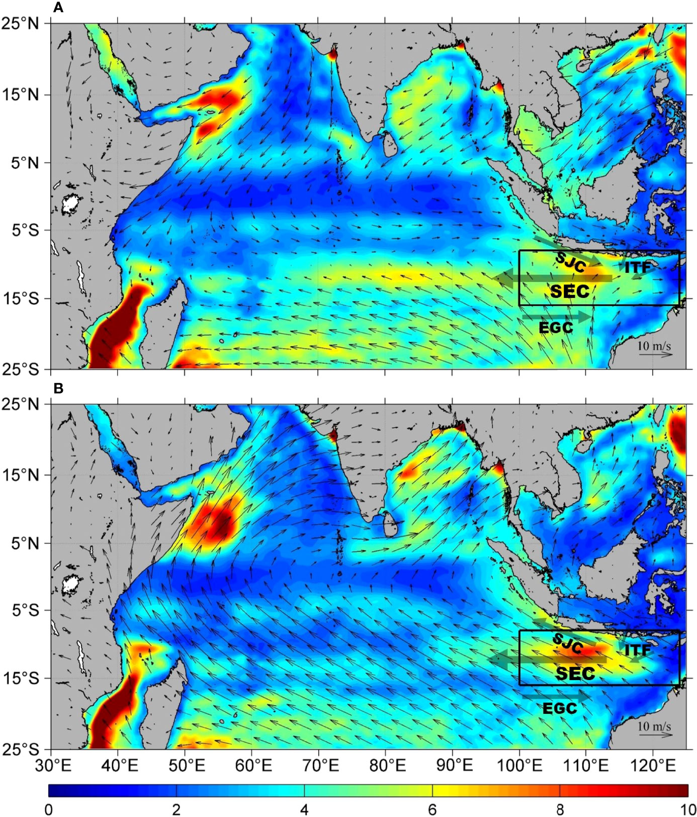
Figure 1 Austral summer [(A); December to February] and winter [(B); June to August] wind (vector; unit: m/s) patterns from ERA5 dataset with overlapping the standard deviation of 30–120 days band-pass–filtered SLA (unit: cm) derived from AVISO in corresponding season. The black box indicates the study area. Primary ocean currents in the study region are shown as semitransparent black solid arrows [revised from Yu and Potemra (2006) and Yang et al. (2015)]: the South Java Current (SJC), the South Equatorial Current (SEC), the Indonesian Throughflow (ITF), and the Eastern Gyral Current (EGC).

Mesoscale eddies are detected in the SETIO by using satellite altimeter surface product and their activities and characteristics are found to be closely related to the ocean currents and thermohaline structure in the region. By analyzing Argo profile data matched to mesoscale eddies, Yang et al. (2015) comprehensively examined the statistical characteristics of mesoscale eddies in the SETIO and found that eddies propagate westward or slightly southward, and the eddy-induced ocean anomalies are mainly confined in upper 300 dbar. They further speculated that the generation of eddies may be related to baroclinic instability of mean circulation. Using the different algorithms, Zhang et al. (2020) and Azis Ismail et al. (2021) detected mesoscale eddies in satellite altimeter SLA fields and presented the characteristics of eddy properties in the SETIO, respectively. They both reported that strong eddies mainly locate in the south side of Java Island. On the basis of the 1½-layer–reduced gravity model, Wang et al. (2021) diagnosed the generation mechanisms of mesoscale eddies and suggested that wind forcing from the tropical Pacific Ocean and nonlinearity plays important roles in eddy generation in the SETIO.

In the several eddy properties, eddy amplitude is one of the most fundamental properties of eddy. As the eddy amplitude increases, hence the rotational velocity and nonlinearity of the eddy increase, the eddy-induced sea surface temperature (SST) anomaly is larger, and its structure converges toward a monopole structure centered close to the eddy sea surface height (SSH) extremum (Gaube et al., 2015), which will further influence the pattern of local air–sea interaction (Sun et al., 2016). In addition, the lager-amplitude eddies induce the stronger current-induced Ekman pumping, which promote nutrients or phytoplankton circulating in eddy interiors (Martin and Richards, 2001; McGillicuddy et al., 2008). By the definition in the work of Chelton et al. (2011b), the eddy amplitude represents how strong the rotational velocity and nonlinearity of an eddy would be; hence, we change it to the more intuitive term “intensity” in this paper. The above findings enrich our understanding on the general properties and characteristics of the eddies in the SETIO, the eddy seasonality, and the underlying mechanisms, however, are yet to be studied considering the strong and unique seasonal variability of ocean in this region. In this study, we will focus on the eddy intensity, investigating its spatial and temporal characteristics on seasonal timescale and underlying mechanisms. The rest of paper is organized as follows. The eddy dataset and ocean reanalysis data are introduced in Section 2. Section 3 describes the spatial distribution and seasonal variation of eddy intensity in the SETIO, and then, the mechanisms responsible for the seasonality of eddy intensity are also revealed. Conclusion and discussion are given in the last section.

2 Data and Methods

2.1 Data

The eddy dataset used in this study is from the Mesoscale Eddy Trajectory Atlas (Ssalto/Duacs, 2020) product in delayed time 2.0 from January 1993 to March 2020, which is distributed by the Archiving, Validation, and Interpretation of Satellite Oceanographic (AVISO). The mesoscale eddies are detected and monitored on the basis of two-satellite daily gridded SLA fields, with an upgraded tracking algorithm. The two-satellite data have more homogeneous resolution of the SLA fields, which is preferable to the temporally varying resolution of the updated series (Chelton et al., 2011b). In the SETIO, some significant differences exist in the eddy statistical characteristics between the upgraded daily AVISO data and the former weekly data, and the eddies detected from the new version of AVISO data are more objective (Yang et al., 2015). The method of eddy identification and tracking is based on SLA fields, which modified from that in the works of Chelton et al. (2011b) and Williams et al. (2011). On each local maximum and minimum of SLA field, the algorithm searches the points around it to extend the area detected as an eddy when it satisfies some criteria. After performing detection on several consecutive days, the trajectories over time of the detected eddies are built by applying a tracking procedure. More details of the detecting and tracking algorithms can be seen in the work of Schlax and Chelton (2016). The dataset includes many eddy parameters, such as eddy centers, radii, amplitudes, rotational velocities, and polarities, which fully meet the requirements of this study. In this study, the eddies from January 1993 to December 2019 are selected to analyze the spatial distribution and seasonal variation of eddy intensity in the SETIO. The eddy intensity is defined as the magnitude of difference between the average SSH at eddy boundary and the extreme value of SSH in eddy interior (Chelton et al., 2011b).

Asia and Indian-Pacific Ocean (AIPOcean2.0) reanalysis dataset (Yan et al., 2010; Yan et al., 2015) is employed to explore the mechanisms of the seasonality of eddy intensity. The ocean data assimilation system of AIPOcean2.0 is based on an eddy-resolving Hybrid Coordinate Ocean Model (HYCOM; Bleck, 2002). The hybrid vertical coordinates can represent the ocean flow better due to the application of different vertical coordinates at different depths (Bleck, 2002). The AIPOcean2.0 covers the Indian Ocean and western Pacific (28°S–44°N, 30°–180°E) with the horizontal resolution of about 1/5°×1/5° and 33 vertical layers from 5 to 5,500 m. Each layer has different thickness. The thickness varies from 5 to 50 m in upper 300 m and from 100 m to 250 m in the layer of 300~2,000 m. The thickness between in the layers deeper than 2,000 m is 500 m. Various types of observations including in situ temperature and salinity profiles (from Argo, conductivity–temperature–depth, Tropical Atmosphere Ocean Project, and expendable bathythermograph), remotely sensed SST, and altimetry data are assimilated into the HYCOM via the Ensemble Optimal Interpolation (EnOI; Oke et al., 2008) to create the AIPOcean2.0 (Yan et al., 2010; Yan et al., 2015). The assimilation method of EnOI uses an ensemble taken from the model simulations to estimate the background error covariance that may allow more anisotropic and inhomogeneous patterns, which tends to improve the model results in a moderate way (Fu et al., 2009). Compared with its former version, the configurations of the model are redesigned and more quality-controlled ocean temperature and salinity profiles are assimilated; thus, the performance of AIPOcean2.0 is greatly improved. AIPOcean2.0 dataset includes the daily three-dimensional temperature, salinity, and current fields as well as the SSH from January 1, 1993, to December 31, 2012. AIPOcean2.0 dataset has been widely used in many studies on mesoscale eddies (e.g., Chen et al., 2012; Vidya and Prasanna Kumar, 2013; Zu et al., 2013; Khan et al., 2021). The daily two-satellite merged SLA data (Pujol and Mertz, 2022) with horizonal resolution 1/4° × 1/4° from AVISO are utilized for data verifying AIPOcean2.0 dataset.

In addition, the surface wind field in monsoon seasons is from the ERA5 data published by ECMWF (Hersbach et al., 2020). The ERA5 data have spatial resolution 1/4°×1/4° and monthly temporal resolution. The monsoonal wind patterns in Figure 1 are calculated from January 1993 to December 2020 in ERA5 data.

2.2 Methods

Energy analysis is used to analyze the energy transfer between the mean and eddy potential and kinetic energies. Following the work of Böning and Budich (1992), eddy kinetic energy (EKE) and eddy available potential energy (EPE) per unit mass are defined as follows:

$$EKE=\frac{1}{2}(u^{\prime 2}+{v^{\prime 2}}^{}),$$

$$EPE=-\frac{g{{\tilde{\rho }}^{\prime 2}}^{}}{2\rho \left(\frac{\partial {\overline{\rho }}_{\theta }}{\partial z}\right)},$$

Where $\tilde{\rho }(x,y,z,t)=\rho (x,y,z,t)-{\rho }_b(z)$, ρ_b(z) is the background density profile from AIPOcean2.0 dataset taken as the annual and horizontal mean within the SETIO, and ${\overline{\rho }}_{\theta }(z)$ is the annual and horizontal mean potential density.

To diagnose the interaction between the eddy and mean flow, the baroclinic conversion rate (BCR) and the barotropic conversion rate (BTR) in the energy budget are defined as (Böning and Budich, 1992; Zhang et al., 2016):

$$BCR=-\frac{g}{\rho \left(-\frac{\partial {\overline{\rho }}_{\theta }}{\partial z}\right)}(\overline{u^{\prime }{\tilde{\rho }}^{\prime }}\frac{\partial \overline{\tilde{\rho }}}{\partial x})+\overline{v^{\prime }{\tilde{\rho }}^{\prime }}\frac{\partial \overline{\tilde{\rho }}}{\partial y}) \text{and}$$

$$BTR=-\left(\overline{u^{\prime }{u}^{\prime }}\frac{\partial \overline{u}}{\partial x}+\overline{u^{\prime }{v}^{\prime }}\left(\frac{\partial \overline{v}}{\partial x}+\frac{\partial \overline{u}}{\partial y}\right)+\overline{v^{\prime }{v}^{\prime }}\frac{\partial \overline{v}}{\partial y}\right).$$

BCR represents the conversion rate between mean potential energy (MPE) and EPE, and BTR is the work of the Reynolds stress against the mean shear, namely, the conversion rate between mean kinetic energy (MKE) and EKE. Positive BCR (BTR) implies part of the MPE (MKE) of the mean flow is transferred to the EPE (EKE) due to the baroclinic (barotropic) instability.

On the basis of the reanalysis dataset AIPOcean2.0, transient components of velocity and density (e.g., u’) are defined as variability of periods between 30 and 120 days, and the residual low-frequency variations with periods larger than 120 days (e.g., ū) are treated as the basic state.

3 Results

3.1 Seasonality of Eddy Intensity

We first examine the seasonality of eddy intensity in the SETIO with focus on its spatial distribution and temporal variation. To figure out the area that has the strongest seasonal variability in the SETIO, we divide the region (90°–125°E, 5°–20°S) into regular small grids (0.5° × 0.5°) and then calculate the average intensity of the eddies in each grid for each calendar month using the Mesoscale Eddy Trajectory Atlas product to obtain the monthly spatial distribution of eddy intensity (Figure 2) . One can see that the eddy intensity is generally homogenous in the region during the first half of the year, but starting from August, the eddy intensity in the area (9.5°–14.5°S, 98°–118°E) to the southwest of Java Island tends to enhance in the following season and peaks in October. The black rectangular box in Figure 2J indicates the strong seasonality area where eddy exhibits most significant seasonal variation. The eddy intensity averaged over the strong seasonality area is then plotted in Figure 2M, and the enhancement of eddy intensity in the second half of the year and its peak in October are clearly demonstrated. The maximum intensity is 12.4 cm, about 1.7 times larger than the minimum value. The seasonal difference of eddy intensity is meaningful because it can represent the change in background. For instance, change of EKE calculated from AVISO in the background follows the variation of eddy intensity. The AVISO EKE averaged in the strong seasonality area reaches the peak in October, and the value is 2,900 cm²/s². It is about 1.3 times larger than the minimum value, which is close to that in eddy intensity.

FIGURE 2

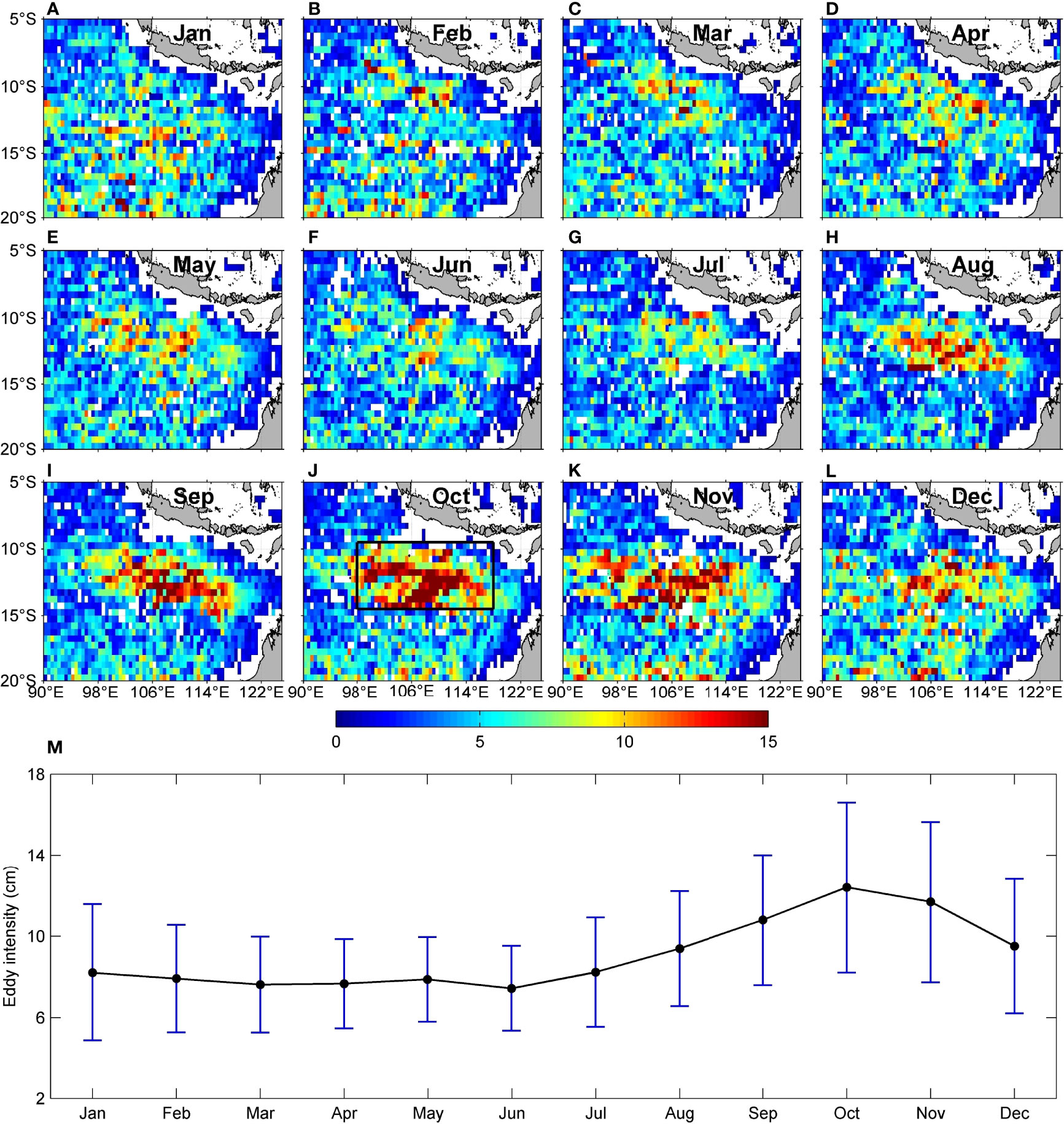
Figure 2 (A–L) Spatial distribution of eddy intensity (unit: cm) of each calendar month, and (M) seasonal variation of eddy intensity averaged in the black rectangular box (9.5°–14.5°S, 98°–118°E) shown in (J). The error bars in (M) show the standard deviation of eddy intensity in every grid.

To explore the underlying mechanisms of the seasonal variation of eddy intensity, the data of temperature, salinity, and current below the sea surface are necessary for the analysis of ocean dynamics. The basic seasonal features of eddy intensity in AIPOcean2.0 dataset is verified in Supplementary Materials. Next, we will examine the vertical structure of eddies of the AIPOcean2.0 dataset in two typical seasons, “strong eddy season” (from September to November) and “weak eddy season” (from February to July) through composite analysis. The theme of composite analysis is that the AIPOcean2.0 dataset is extracted in space and time to follow each eddy firstly and then collecting their subsurface current and hydrographic conditions. Following the eddy composite method by Zu et al. (2019), 4° × 4° fields are extracted from the temperature and salinity anomalies (TS anomalies) at the center of each eddy, and composite plots can then be obtained separately by averaging the extracted fields according to eddy polarities. Figures 3A, B show the composite vertical profiles of TS anomalies in the upper layer of ocean, and it can be found that the maximal values of temperature anomalies in both typical seasons are at about 100 m depth, where the thermocline is located, and the mean magnitude is about 1.3°C. Similar seasonal difference can also be found in the vertical profiles of the salinity anomalies. Same composite method is also applied to the current velocity fields associated with eddies, and one can find in Figures 3C–F that the most energetic currents appear in upper 100 m, with maximal speed in the surface, and the maxima is about 20 cm/s in strong eddy season and around 10 cm/s in weak eddy season. Like as TS anomalies, the seasonal difference in eddy induced current anomaly is also prominent in the upper 500 m. The composite maps illustrate that the AIPOcean2.0 dataset can capture the mesoscale eddy in subsurface layer well.

FIGURE 3

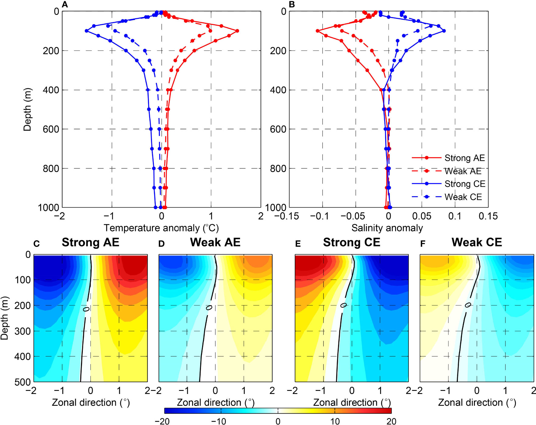
Figure 3 (A) Composite vertical profiles of the temperature anomaly (unit: °C) and (B) salinity anomaly associated with eddies. The solid and dashed lines are the profiles in strong and weak eddy seasons, respectively. The red and blue colors are for AEs and CEs, respectively. (C–F) Composite maps of meridional current (unit: cm/s) on the vertical section across eddy center for AEs and CEs in the two typical seasons. The positive/negative values stand for northward/southward flows.

3.2 Evolution of Eddy Intensity in Its Lifetime

The mesoscale eddies in the ocean always keep moving and evolving during their lifetime since they were formed. This is also confirmed by the statistical analysis on eddies in the SETIO by Yang et al. (2015), which shows that most of eddies propagate westward and can move 200–600 km during their lifetime (average life span is about 2 months). Therefore, tracing the movement of eddies and study their magnitude change is a key step to explore the underlying mechanisms of the seasonality of eddy intensity. Figure 4 shows the magnitude variations in the lifetime of eddies formed in each calendar month. It is interesting to note that the magnitude of eddies formed in January through May have barely significant growth in the next few months and their life span is relatively short. Starting from June, eddies exhibit continuously growth after their formation, and this feature is especially prominent for eddies formed in July to September (Figures 4G–I). It is worthy to note that the magnitude of eddies formed in this season grows most rapidly and continuously during the following 3 months and peaks in October or October to November. The eddies generated in October grow most rapidly in this month but weaken after October. The change in magnitude of the eddies generated after October, however, shows a similar characteristic to those formed before June.

FIGURE 4

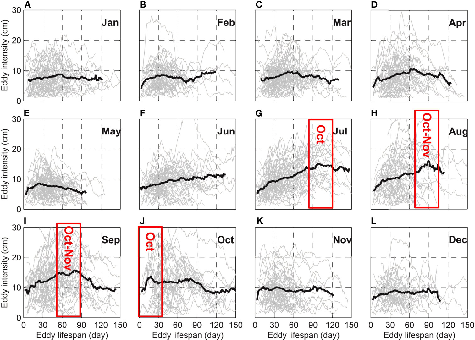
Figure 4 Variation of the magnitude of eddies formed in each calendar month (A–L) during their lifetime. Gray lines represent individual eddies, and black lines are the means. Only eddies with life span longer than 30 days are plotted. Each panel not only shows the monthly results but also contains information regarding the evolution of eddy intensity for the next 4 months. The red box marks the peak of eddy intensity and corresponding month.

The trajectories of the eddies generated in the austral summer (January, February, and March) and the austral winter (July, August, and September) display the spatial evolution of eddies more intuitive, which show the distinct seasonal difference for the relative strong eddies (the eddies with intensity larger than 15 cm, which is main contributor of the seasonal variation of eddy intensity): the eddies are sparse with weaker intensity in austral summer (Figure 5A); however, in austral winter, more eddies are generated and the eddy intensity increase markedly within eddy migration (Figure 5B). These eddies generally attain the strongest when they move into the strong seasonality area. About 72% of the eddies passed though the strong seasonality area in October form before October (Figure 6A), in which the eddies generated in austral winter account for 63% (Figure 6B). The spatial evolution of eddies further illustrates that the eddies in the strong seasonality area are the results of the continuous movement and growth of the eddies generated in the months before October.

FIGURE 5

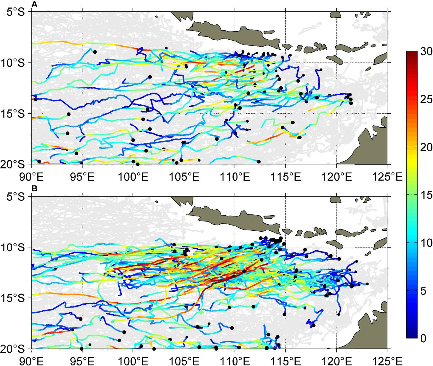
Figure 5 Trajectories of eddies generated in austral summer (A) and austral winter (B), respectively. The eddies with intensity (unit: cm) smaller than 15 cm are marked by gray curves, whereas the eddies with intensity larger than 15 cm are showed by color curves. The gray and black dots indicate the locations of eddy generation.

FIGURE 6

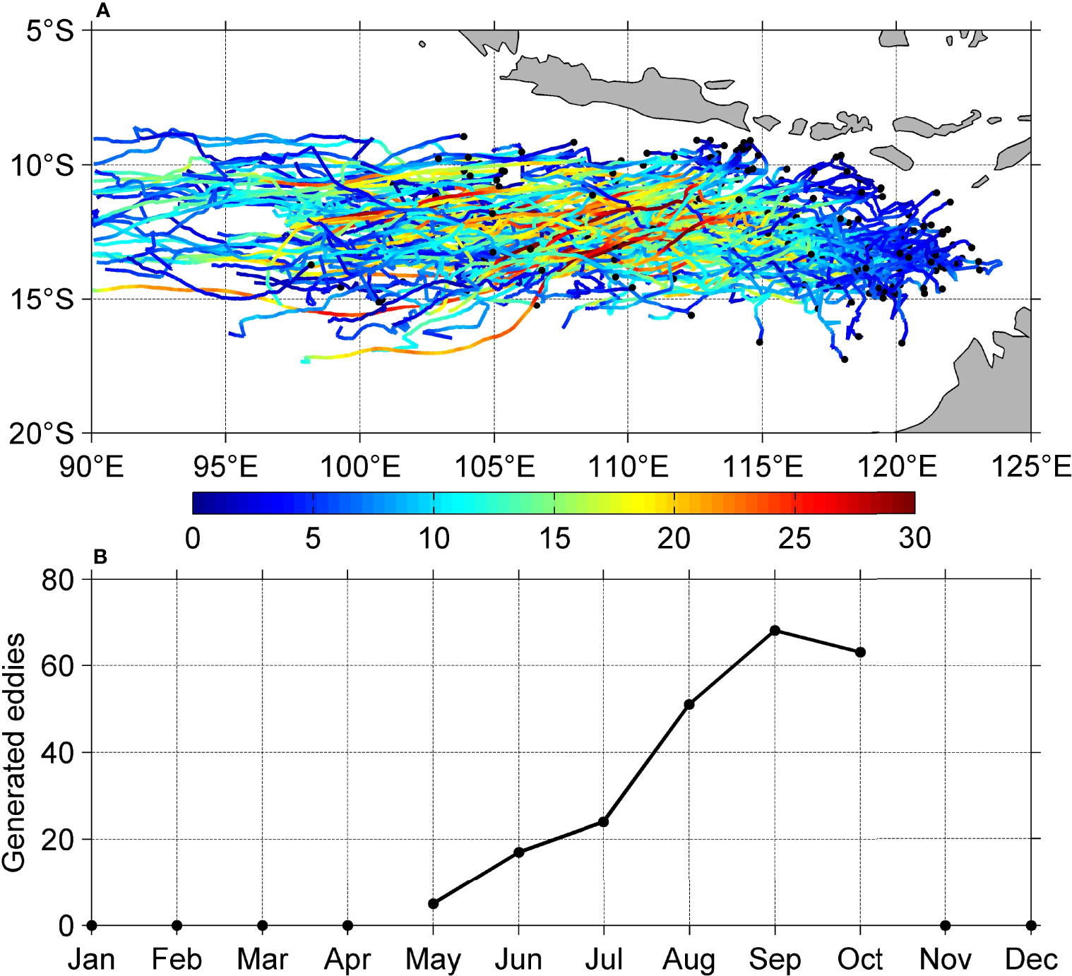
Figure 6 Same as Figure 5 but for eddies passed through the strong seasonality area in October. (B) Variation of the number of generated eddies in (A).

Actually, the intraseasonal variabilities discussed by Feng and Wijffels (2002) and Yu and Potemra (2006) are mainly caused by the seasonality of the mesoscale eddy intensity in this region, and the westward intraseasonal signal is primarily due to the propagation of mesoscale eddies. On the basis of previous studies, the seasonality of eddy intensity is controlled by the variability in background field. However, the physical mechanism among them is still need to be investigated.

3.3 Mechanism of the Seasonality in Eddy Intensity

Mesoscale eddies absorb energy to survive in their migration, in which the energy conversion is through the oceanic instabilities (Robinson and Mcwilliams, 1974). The oceanic instabilities primarily include barotropic instability and baroclinic instability. To evaluate the effects of barotropic instability and baroclinic instability, the BTR and BCR are calculated. By using the model output and the method of energy analysis, Wang et al. (2021) calculate the annual mean BTR and BCR in SETIO and points out that both barotropic instability and baroclinic instability have important impacts on eddy generation. Their results are somewhat different from those in the study by Yu and Potemra (2006), in which BTR is stronger than BCR. Therefore, the impact of seasonal variation in oceanic unstable processes on eddy intensity is examined in this section.

On the basis of the AIPOcean2.0 data and the method of energy analysis, we further examine the seasonal effect of energy in background field on eddy intensity. For comparison, we firstly calculate the annual mean BTR and BCR overlapping EKE and EPE, respectively (Figure S3). Vertically integrated EKE and EPE are high not only in the strong seasonality area but also along the southern Sumatra–Java coast (Figures S3A, B). Comparing Figure S3B against Figure S3C, EPE dominates the total eddy energy (TEE, sum of EKE and EPE). The spatial distributions of EKE and EPE are consistent with the results in the work of Wang et al. (2021), whereas the magnitude in EKE is relatively smaller. Then, we take the average in the sub-region (10°–14°S, 105°–115°E) in the strong seasonality area with high values of BTR and BCR and obtain their seasonal variations in the vertical distribution (Figure 7). The results are not sensitive with a changing sub-region. BTR and BCR both show remarkable but very different seasonal characteristics. BTR starts to strengthen in July, reaching the strongest in September, and rapidly declines from October. The seasonal changes focus on the water depth shallower than 30 m, indicating that the barotropic instability mainly occurs in the mixing layer. Compared with the BTR, the most significant difference is that the seasonal variation in BCR is primarily concentrated at a depth of 75~175 m, with a longer duration of large BCR, which begins to enhance in August, attaining its peak in September to October, and then gradually weakens. The maximum value in the BCR is about three times greater than that in the BTR. An important fact should be noted that BTR begins to enhance in July and reaches the peak in September, occurring 1 month earlier than that of BCR.

FIGURE 7

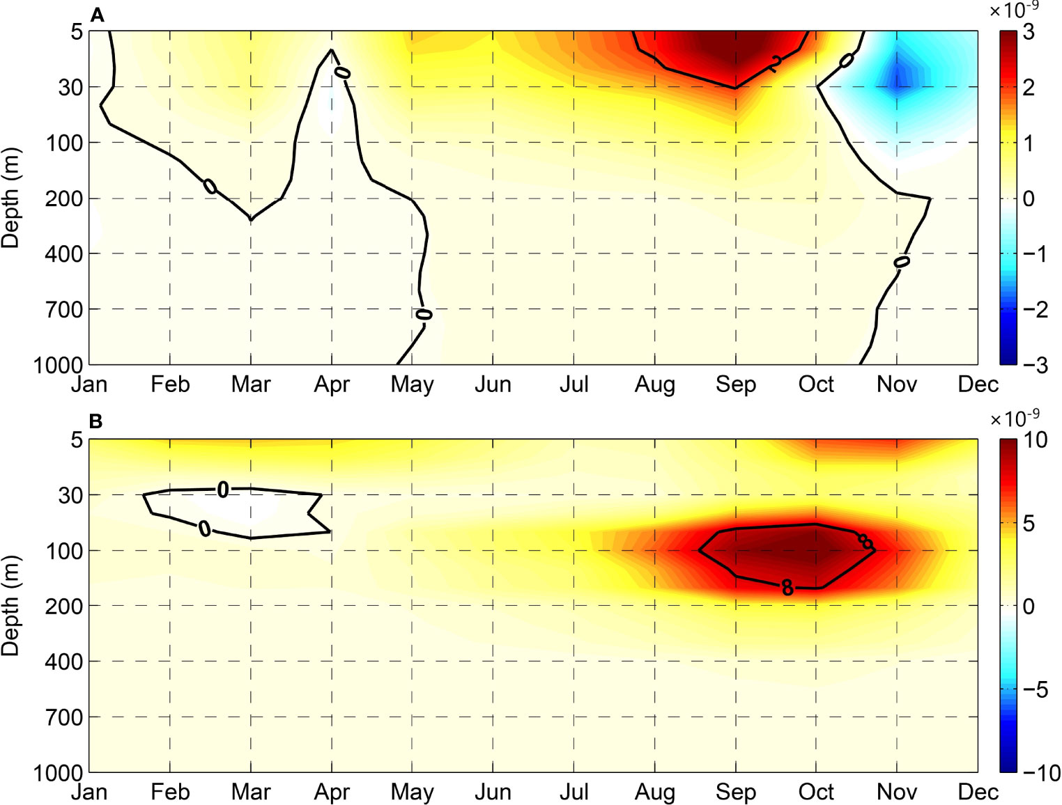
Figure 7 Seasonal variation of BTR (A) and BCR (B) averaged in the area (10°–14°S, 105°–115°E). Units for BTR and BCR are m²/s³.

In south small region (9°–10°S, 112°–115°E) of Lombok Strait, where many strong eddies origin (Figure 5), the seasonal variations in BTR and BCR are similar to that in the strong seasonality area, in which the variation of BTR also occurs 1 month earlier than that of BCR. However, the baroclinic instability is confined to the mixing layer (figure not shown). In this region, the BTR timely provides energy for generating eddies by transforming the average kinetic energy to EKE in austral winter. Therefore, at the stage of eddy formation, the barotropic instability play more important role in promoting the generation of eddies.

After eddies were generated, most of them migrate to the strong seasonality area in October, when the background field happens to occur the strongest BCR (Figure 7B). More sufficient energy is provided for the eddy growth through the strongest BCR. Different from the role of BTR in the strong seasonality area, the BCR is the protagonist, which supply enough energy for eddy development by converting the average potential energy to EPE in September to October. Comparing Figure 2M against Figure 7B, as expected, it can be found that the seasonal variation of eddy intensity follows that of BCR. As a result, the eddy intensity is significantly strengthened in this period, characterizing by large amplitude and then capturing by altimeter satellites.

In November and December, the background field in the strong seasonality area changes largely, mainly showing that oceanic unstable processes weaken. Because of the barren dynamic environment, the marine background field cannot feed enough energy for sustaining eddy development, and then, the eddy intensity reduces. Although the strong eddies in October is evolved as a result of the propagation of eddies generated in previous months, October is crucial, because BCR and BTR in this month concurrently supply the needed energy for eddy development.

The key physical factors that control the seasonal characteristics in these unstable processes will be further analyzed next. We define the depth of 1,025 kg/m³ isopycnal (D25) denoting the pycnocline depth. Because of the effect of upwelling in austral winter, which causes the cold water in lower depth to rise up and then the pycnocline elevates. The D25 tends to decrease from south to north, indicating that the pycnocline slopes in the north side, which can be described by the meridional change of the pycnocline. Figures 8A, B display the meridional gradient of D25 (∂D25/∂y) in austral summer and winter, respectively. In this figure, obvious seasonal differences of the pycnocline can be seen. The ∂D25/∂y is small, and there is no large difference in distribution across the whole region in austral summer. However, in austral winter, the ∂D25/∂y shows a strong seasonal variability. Except for the areas near several straits, the high value region (absolute value) is located in the range of 10°–13°S and 105°–120°E and begins to decrease rapidly in the regions south of 12°S and weaken significantly in the regions west of 110°E. As shown in Figure 5B, the source area of eddy generation is basically located in the southwestern side of Lombok strait and within the range of 115°–120°E.

FIGURE 8

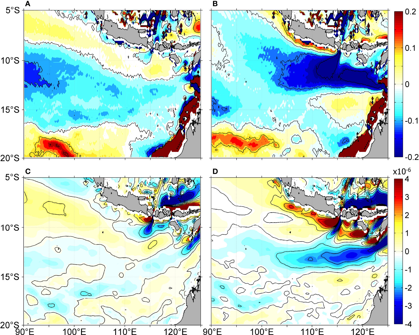
Figure 8 Seasonal characteristics of dynamic environment in the background in austral summer (B, D) and austral winter (A, C), respectively. (A, B) denote the meridional gradient of D25 (unit: m/km), in which the interval of contour lines is 0.1 m/km. (C, D) represent the meridional gradient of zonal current (unit: s⁻¹) averaged in upper 30 m, in which the contour lines denote the value of 0.

Compared with the calculation formula of BCR, it is not difficult to find that BCR largely depends on the horizontal gradient of the density. Because the zonal gradient of D25 is small (figure not shown), the ∂D25/∂y basically represents the density gradient, namely, BCR is essentially subject to the ∂D25/∂y. In the region with drastic changes of the ∂D25/∂y, the potential energy and BCR increase markedly (Figure S3B). This suggests that sloping of the pycnocline induced by seasonal upwelling can noticeably enhance the meridional gradient of density, which is the main factor of inducing baroclinicity variation.

In addition to pycnocline, ocean current also shows the seasonal variability. As shown in Figures 8C, D, the meridional gradient of zonal current (∂u/∂y) is significantly enhanced in austral winter. Except for the areas around the straits, the ∂u/∂y in austral summer is generally smaller in the whole region (Figure 8C). However, in austral winter, it is significantly reinforced in the east of 105°E and the latitudinal zone 11°~14.5°S (Figure 8D), which covering the most areas where larger EKE occurs. Besides, the magnitude of the zonal gradient (∂u/∂x) and the gradient of the meridional current (dv) is smaller and the seasonal difference is weaker (figures not shown). Therefore, the seasonal variability of the barotropic unstable process mainly depends on the change of ∂u/∂y in the strong seasonality area.

4 Conclusion and Discussion

In this study, the seasonality of mesoscale eddy intensity in the SETIO and its mechanisms are examined using the latest eddy dataset and oceanic hydrologic reanalysis data. The results show that the eddy intensity in an area to the southwest coast of the Java Island has prominent seasonality—eddies in this area are relatively weak during the first half of the year but tend to enhance in August and peak in October. By analyzing the evolution of the eddy intensity during its lifetime, it is found that the strongest eddies in October are actually developed from the ones mainly formed in July to September.

The seasonal feature of the unstable processes in the local background field determines the seasonal variability of the energy supply for eddy generation and development. Energy analysis demonstrates that the BTR and BCR both have obvious seasonal variations in this region, which play a different role at different development stages. By transforming the average kinetic energy to EKE in the austral winter, the barotropic instability timely provides energy for generating eddies, mostly focusing on mixing layer. After eddies were formed in the austral winter, most of them move westward/southwestward and the baroclinic instability supplies enough energy for eddy development by converting the average potential energy to EPE from September to October, primarily concentrating at a depth of 75~175 m. In November and December, the oceanic unstable processes weaken and then the eddy intensity reduces. Further analysis shows that the pycnocline and the meridional gradient of the zonal current are the key physical factors that determine the baroclinic and barotropic processes in the SETIO, respectively.

The activities of energic eddies can directly alter the SSH, enhancing the variance of SLA. In essential, the intraseasonal variabilities discussed by Feng and Wijffels (2002) and Yu and Potemra (2006), as mentioned above, are principal a form of energic eddies effect on SSH. Compared with the energy in SLA, the energy represented by the tracked long-lived eddies (>4 weeks) is coherent in structure, which is more conducive to studying the spatiotemporal evolutionary characteristics in the tracers’ anomalies associated with mesoscale eddies. However, it should be noted that, in the areas with high SLA, more energic mesoscale eddies may not exist, because the strong currents or other marine dynamic processes can also induce the fluctuations of sea level.

Throughout this study, we have documented the role of barotropic instability and baroclinic instability in the seasonal variation of the mesoscale eddy intensity. The key physical processes controlling the barotropic instability and baroclinic instability in background induced by the zonal current and pycnocline are clarified. The results of this paper not only help in understanding the mechanisms of the generation and development of mesoscale eddies but also play an important role in the prediction of local marine ecological processes and fishery production associated with eddies. In addition, the effect of the seasonality in eddy intensity on local climate change in this region is also an interesting topic for future research.

Data Availability Statement

The altimetric Mesoscale Eddy Trajectory Atlas Products are produced by SSALTO/DUACS and distributed by AVISO+ (https://www.aviso.altimetry.fr/) with support from CNES, in collaboration with Oregon State University with support from NASA. The SLA data is from Copernicus Marine Environment Monitoring Service (CMEMS) (https://marine.copernicus.eu/). The AIPOcean2.0 dataset is distributed by the South China Sea and Adjacent Seas Data Center, National Earth System Science Data Center, National Science & Technology Infrastructure of China (http://ocean.geodata.cn/index.html). More inquiries can be directed to the corresponding authors.

Author Contributions

YZ performed the data analysis, wrote the initial draft and modified the manuscript. YF proposed the main ideas and modified the manuscript. SS, GY, LG and YD participated to the discussions and contributed to the improvement of the manuscript. All authors contributed to the article and approved the submitted version.

Funding

This work is supported by Global Change and Air-Sea Interaction Program (GASI-04-QYQH-03, GASI-01-WINDSTwin), the Basic Scientific Fund for National Public Research Institutes of China (2018S02), the National Key R&D Program of China (2018YFA0605701, 2019YFC1509102), the National Natural Science Foundation of China (41876030, 41976021, 41606034 and 41876231), the Impact and Response of Antarctic Seas to Climate Change (IRASCC 01-01-01A), the Basic Scientific Fund for National Public Research Institutes of China (2019Q03), Taishan Scholars Project Fund (ts20190963) and the Marine S&T Fund of Shandong Province for Pilot National Laboratory for Marine Science and Technology (Qingdao) (No.2018SDKJ0105-3).

Conflict of Interest

The authors declare that the research was conducted in the absence of any commercial or financial relationships that could be construed as a potential conflict of interest.

Publisher’s Note

All claims expressed in this article are solely those of the authors and do not necessarily represent those of their affiliated organizations, or those of the publisher, the editors and the reviewers. Any product that may be evaluated in this article, or claim that may be made by its manufacturer, is not guaranteed or endorsed by the publisher.

Supplementary Material

The Supplementary Material for this article can be found online at: https://www.frontiersin.org/articles/10.3389/fmars.2022.855832/full#supplementary-material

References

Amores A., Melnichenko O., Maximenko N. (2017). Coherent Mesoscale Eddies in the North Atlantic Subtropical Gyre: 3-D Structure and Transport With Application to the Salinity Maximum. J. Geophys. Res. Ocean. 122 (1), 23–41. doi: 10.1002/jgrc.v122.1

CrossRef Full Text | Google Scholar

Annamalai H., Murtugudde R., Potemra J., Xie S., Liu P., Wang B. (2003). Coupled Dynamics Over the Indian Ocean: Spring Initiation of the Zonal Mode. Deep. Sea. Res. Part II. 50, 2305–2330. doi: 10.1016/S0967-0645(03)00058-4

CrossRef Full Text | Google Scholar

Azis Ismail M. F., Ribbe J., Arifin T., Taofiqurohman A., Anggoro D. (2021). A Census of Eddies in the Tropical Eastern Boundary of the Indian Ocean. J. Geophysic. R. Ocean. 126, e2021JC017204. doi: 10.1029/2021JC017204

CrossRef Full Text | Google Scholar

Bleck R. (2002). An Oceanic General Circulation Model Framed in Hybrid Isopycnic-Cartesian Coordinates. Ocean. Model. 4, 55–88. doi: 10.1016/S1463-5003(01)00012-9

CrossRef Full Text | Google Scholar

Böning C. W., Budich R. G. (1992). Eddy Dynamics in a Primitive Equation Model: Sensitivity to Horizontal Resolution and Friction. J. Physic. Oceanog. 22 (4), 361–381. doi: 10.1175/1520-0485(1992)022<0361:EDIAPE>2.0.CO;2

CrossRef Full Text | Google Scholar

Broeker W. S. (1991). The Great Ocean Conveyor. Oceanography 4, (2), 79–89. doi: 10.5670/oceanog.1991.07

CrossRef Full Text | Google Scholar

Chelton D. B., Gaube P., Schlax M. G., Early J. J., Samelson R. M. (2011a). The Influence of Nonlinear Mesoscale Eddies on Near-Surface Oceanic Chlorophyll. Science 334 (6054), 328–332. doi: 10.1126/science.1208897

PubMed Abstract | CrossRef Full Text | Google Scholar

Chelton D. B., Schlax M. G., Samelson R. M. (2011b). Global Observations of Nonlinear Mesoscale Eddies. Prog. Oceanogr. 91 (2), 167–216. doi: 10.1016/j.pocean.2011.01.002

CrossRef Full Text | Google Scholar

Chelton D. B., Schlax M. G., Samelson R. M., de Szoeke R. A. (2007). Global Observations of Large Oceanic Eddies. Geophys. Res. Lett. 34, L15606. doi: 10.1029/2007GL030812

CrossRef Full Text | Google Scholar

Cheng Y.-H., Ho C.-R., Zheng Q., Kuo N.-J. (2014). Statistical Characteristics of Mesoscale Eddies in the North Pacific Derived From Satellite Altimetry. Remote Sens. 6, 5164–5183. doi: 10.3390/rs6065164

CrossRef Full Text | Google Scholar

Chen L., Jia Y., Liu Q. (2017). Oceanic Eddy-Driven Atmospheric Secondary Circulation in the Winter Kuroshio Extension Region. J. Oceanogr. 73, 295–307. doi: 10.1007/s10872-016-0403-z

CrossRef Full Text | Google Scholar

Chen G., Wang D., Hou Y. (2012). The Features and Interannual Variability Mechanism of Mesoscale Eddies in the Bay of Bengal. Cont. Shelf. Res. 47, 178–185. doi: 10.1016/j.csr.2012.07.011

CrossRef Full Text | Google Scholar

Dong C., McWilliams J. C., Liu Y., Chen D. (2014). Global Heat and Salt Transports by Eddy Movement. Nat. Commun. 5, 3294. doi: 10.1038/ncomms4294

PubMed Abstract | CrossRef Full Text | Google Scholar

Du Y., Qu T., Meyers G., Masumoto Y., Sasaki H. (2005). Seasonal Heat Budget in the Mixed Layer of the Southeastern Tropical Indian Ocean in a High-Resolution Ocean General Circulation Model. J. Geophys. Res. 110, C04012. doi: 10.1029/2004JC002845

CrossRef Full Text | Google Scholar

Feng M., Wijffels S. (2002). Intraseasonal Variability in the South Equatorial Current of the East Indian Ocean. J. Phys. Oceanogr. 32, 265–277. doi: 10.1175/1520-0485(2002)032<0265:IVITSE>2.0.CO;2

CrossRef Full Text | Google Scholar

Frenger I., Gruber N., Knutti R., Münnich M. (2013). Imprint of Southern Ocean Eddies on Winds, Clouds and Rainfall. Nat. Geosci. 6, 608–612. doi: 10.1038/ngeo1863

CrossRef Full Text | Google Scholar

Frenger I., Münnich M., Gruber N. (2018). Imprint of Southern Ocean Mesoscale Eddies on Chlorophyll. Biogeosci. Dis. 15, 4781–4798. doi: 10.5194/bg-15-4781-2018

CrossRef Full Text | Google Scholar

Frenger I., Münnich M., Gruber N., Gruber N., Knutti R. (2015). Southern Ocean Eddy Phenomenology. J. Geophys. Res. Ocean. 120 (11), 7413–7449. doi: 10.1002/2015JC011047

CrossRef Full Text | Google Scholar

Fu W. W., Zhu J., Yan C. X. (2009). A Comparison Between 3DVAR and EnOI Techniques for Satellite Altimetry Data Assimilation. Ocean. Model. 26 (3–4), 206–216. doi: 10.1016/j.ocemod.2008.10.002

CrossRef Full Text | Google Scholar

Gaube P., Chelton D. B., Samelson R. M., Schlax M. G., O’Neill L. W. (2015). Satellite Observations of Mesoscale Eddy-Induced Ekman Pumping. J. Phys. Oceanogr. 45 (1), 104–132. doi: 10.1175/jpo-d-14-0032.1

CrossRef Full Text | Google Scholar

Hersbach H., Bell B., Berrisford P., Hirahara S., Horányi A., Muñoz-Sabater J., et al. (2020). The ERA5 Global Reanalysis. Q. J. R. Meteorol. Soc. 146 (730), 1999–2049. doi: 10.1002/qj.3803

CrossRef Full Text | Google Scholar

Khan S., Song Y., Huang J., Piao S. (2021). Analysis of Underwater Acoustic Propagation Under the Influence of Mesoscale Ocean Vortices. J. Mar. Sci. Eng. 9, 799. doi: 10.3390/jmse9080799

CrossRef Full Text | Google Scholar

Liu Y., Dong C., Guan Y., Chen D., Mcwilliams J. C., Nencioli F. (2012). Eddy Analysis in the Subtropical Zonal Band of the North Pacific Ocean. Deep. Sea. Res. 68, 54–67. doi: 10.1016/j.dsr.2012.06.001

CrossRef Full Text | Google Scholar

Martin A., Richards K. (2001). Mechanisms for Vertical Nutrient Transport Within a North Atlantic Mesoscale Eddy. Deep-Sea. Res. II. 48, 757–773. doi: 10.1016/S0967-0645(00)00096-5

CrossRef Full Text | Google Scholar

Masumoto Y., Yamagata T. (1996). Seasonal Variations of the Indonesian Throughflow in a General Ocean Circulation Model. J. Geophys. Res. Ocean. 101 (C5), 12287–12293. doi: 10.1029/95JC03870

CrossRef Full Text | Google Scholar

McGillicuddy, Ledwell J., Anderson L. (2008). Response to Comments on ‘‘Eddy/wind Interactions Stimulate Extraordinary Mid-Ocean Plankton Blooms.’’. Science 320, 488. doi: 10.1126/science.1148974

CrossRef Full Text | Google Scholar

Melnichenko O., Amores A., Maximenko N., Hacker P., Potemra J. (2017). Signature of Mesoscale Eddies in Satellite Sea Surface Salinity Data. J. Geophys. Res. Ocean. 122, 1416–1424. doi: 10.1002/2016JC012420

CrossRef Full Text | Google Scholar

Meyers G., Bailey R. J., Worby A. P. (1995). Geostrophic Transport of the Indonesian Throughflow. Deep. Sea. Res. 42, 1163–1174. doi: 10.1016/0967-0637(95)00037-7

CrossRef Full Text | Google Scholar

Molcard R., Fieux M., Syamsudin F. (2001). The Throughflow Within Ombai Strait. Deep. Sea. Res. Part II. 48, 1237–1253. doi: 10.1016/S0967-0637(00)00084-4

CrossRef Full Text | Google Scholar

Murray S. P., Arief D. (1988). Throughflow Into the Indian Ocean Through the Lombok Strait. Nature 333, 444–447. doi: 10.1038/333444a0

CrossRef Full Text | Google Scholar

Oke P. R., Brassington G. B., Griffin D. A., Schiller A. (2008). The Bluelink Ocean Data Assimilation System (BODAS). Ocean. Model. 21, 46–70. doi: 10.1016/j.ocemod.2007.11.002

CrossRef Full Text | Google Scholar

Pujol M.-I., Mertz Françoise (2022). Product User Manual for Sea Level Products. Copernicus Marine Environment Monitoring Service (CMEMS). product 4.1, 1–36. doi: 10.48670/moi-00148

CrossRef Full Text | Google Scholar

Qu T., Meyers G. (2005). Seasonal Characteristics of Circulation in the Southeastern Tropical Indian Ocean. J. Physic. Oceanog. 35, 255–267. doi: 10.1175/JPO-2682.1

CrossRef Full Text | Google Scholar

Robinson A. R., Mcwilliams J. C. (1974). The Baroclinic Instability of the Open Ocean. J. Physic. Oceanog. 4 (3), 281–294. doi: 10.1175/1520-0485(1974)004<0281:TBIOTO>2.0.CO2

CrossRef Full Text | Google Scholar

Schlax M. G., Chelton D. B. (2016). The “Growing Method" of Eddy Identification and Tracking in Two and Three Dimensions (Corvallis, Oregon: College of Earth, Ocean and Atmospheric Sciences, Oregon State University).

Google Scholar

Schott F. A., Xie S. P., McCreary J. P. (2009). Indian Ocean Circulation and Climate Variability. Rev. Geophys. 47, 1–46. doi: 10.1029/2007RG000245

CrossRef Full Text | Google Scholar

Ssalto/Duacs (2020) Mesoscale Eddy Trajectory Atlas Product Handbook. Available at: https://www.aviso.altimetry.fr/fileadmin/documents/data/tools/hdbk_eddytrajectory.pdf.

Google Scholar

Sun S., Fang Y., Liu B., Tana (2016). Coupling Between SST and Wind Speed Over Mesoscale Eddies in the South China Sea. Ocean. Dyn. 66 (11), 1467–1474. doi: 10.1007/s10236-016-0993-4

CrossRef Full Text | Google Scholar

Sun S., Fang F., Zu Y., Liu B., Tana, Azizan A. S. (2020). Seasonal Characteristics of Mesoscale Coupling Between the Sea Surface Temperature and Wind Speed in the South China Sea. J. Clim. 33 (2), 625–638. doi: 10.1175/JCLI-D-19-0392.1

CrossRef Full Text | Google Scholar

Susanto R. D., Gordon A. L., Zheng Q. N. (2001). Upwelling Along the Coasts of Java and Sumatra and its Relation to ENSO. Geophysic. Res. Lett. 28, 1599–1602. doi: 10.1029/2000GL011844

CrossRef Full Text | Google Scholar

Vidya P. J., Prasanna Kumar S. (2013). Role of Mesoscale Eddies on the Variability of Biogenic Flux in the Northern and Central Bay of Bengal. J. Geophysic. Res. Ocean. 118, 5760–5771. doi: 10.1002/jgrc.20423

CrossRef Full Text | Google Scholar

Wang X., Cheng X., Liu X., Chen D. (2021). Dynamics of Eddy Generation in the Southeast Tropical Indian Ocean. J. Geophysic. Res. Ocean. 126, e2020JC016858. doi: 10.1029/2020JC016858

CrossRef Full Text | Google Scholar

Wijffels S. E., Bray N. A., Hautala S., Meyers G., Morawitz W. M. L. (1996). The WOCE Indonesian Throughflow Repeat Hydrography Sections: I10 and IR6. Int. WOCE. Newsl. 24, 25–28.

Google Scholar

Williams S., Petersen M., Bremer P.-T., Hecht M., Pascucci V., Ahrens J., et al. (2011). Adaptive Extraction and Quantification of Geophysical Vortices. IEEE T. Vis. Comput. Gr. 17, 2088–2095. doi: 10.1109/TVCG.2011.162

CrossRef Full Text | Google Scholar

Wyrtki K. (1973). An Equatorial Jet in the Indian Ocean. Science 181, 262–264. doi: 10.1126/science.181.4096.262

PubMed Abstract | CrossRef Full Text | Google Scholar

Yang G., Wang F., Li Y., Lin P. (2013). Mesoscale Eddies in the Northwestern Subtropical Pacific Ocean: Statistical Characteristics and Three-Dimensional Structures. J. Geophys. Res. Ocean. 118, 1906–1925. doi: 10.1002/jgrc.20164

CrossRef Full Text | Google Scholar

Yang G., Yu W., Yuan Y., Zhao X., Wang F., Chen G., et al. (2015). Characteristics, Vertical Structures, and Heat/Salt Transports of Mesoscale Eddies in the Southeastern Tropical Indian Ocean. J. Geophysic. Res. Ocean. 120, 6733–6750. doi: 10.1002/2015JC011130

CrossRef Full Text | Google Scholar

Yang G., Zhao X., Li Y., Liu L., Wang F., Yu W. (2019). Chlorophyll Variability Induced by Mesoscale Eddies in the Southeastern Tropical Indian Ocean. J. Mar. Syst. 199, 103209. doi: 10.1016/j.jmarsys.2019.103209

CrossRef Full Text | Google Scholar

Yan C. X., Zhu J., Xie J. P. (2010). An Ocean Reanalysis System for the Joining Area of Asia and Indian Pacific Ocean. Atmos. Ocean. Sci. Lett. 3, 81–86. doi: 10.1080/16742834.2010.11446848

CrossRef Full Text | Google Scholar

Yan C. X., Zhu J., Xie J. P. (2015). An Ocean Data Assimilation System in the Indian Ocean and West Pacific Ocean. Adv. Atmos. Sci. 32 (11), 1460–1472. doi: 10.1007/s00376-015-4121-z

CrossRef Full Text | Google Scholar

Yu Z., Potemra J. (2006). Generation Mechanism for the Intraseasonal Variability in the Indo-Australian Basin. J. Geophysic. Res. Ocean. 111, 1–11. doi: 10.1029/2005JC003023

CrossRef Full Text | Google Scholar

Zhang N., Liu G., Liu Q., Zheng S., Perrie W. (2020). Spatiotemporal Variations of Mesoscale Eddies in the Southeast Indian Ocean. J. Geophysic. Res. Ocean. 125, e2019JC015712. doi: 10.1029/2019JC015712

CrossRef Full Text | Google Scholar

Zhang Z., Tian J., Qiu B., Zhao W., Chang P., Wu L., et al. (2016). Observed 3D Structure, Generation, and Dissipation of Oceanic Mesoscale Eddies in the South China Sea. Sci. Rep. 6, 24349. doi: 10.1038/srep24349

PubMed Abstract | CrossRef Full Text | Google Scholar

Zhang Z., Wang W., Qiu B. (2014). Oceanic Mass Transport by Mesoscale Eddies. Science 345 (6194), 322–324. doi: 10.1126/science

PubMed Abstract | CrossRef Full Text | Google Scholar

Zhang Z., Zhang Y., Wang W., Huang R. X. (2013). Universal Structure of Mesoscale Eddies in the Ocean. Geophys. Res. Lett. 40, 3677–3681. doi: 10.1002/grl.50736

CrossRef Full Text | Google Scholar

Zu Y., Sun S., Zhao W., Li P., Liu B., Fang Y., et al. (2019). Seasonal Characteristics and Formation Mechanism of the Thermohaline Structure of Mesoscale Eddy in the South China Sea. Acta Oceanol. Sin. 38 (4), 29–38. doi: 10.1007/s13131-018-1222-4

CrossRef Full Text | Google Scholar

Zu T., Wang D., Yan C., Igor B., Zhuang W., Chen J. (2013). Evolution of an Anticyclonic Eddy Southwest of Taiwan. Ocean. Dyn. 63 (5), 519–531. doi: 10.1007/s10236-013-0612-6

CrossRef Full Text | Google Scholar