Movements and Diving Behavior of the Eastern North Pacific Offshore Killer Whale (Orcinus orca)

The Pacific Offshore killer whale population is currently listed as data deficient on the IUCN Red List and Threatened in Canada. The population is estimated at 300 individuals with a range extending from Southern California to the Aleutian Islands in Alaska. Only 157 encounters with this ecotype have been photo-documented between 1988 and 2014; consequently, movement and behavioral data are limited and restricted to areas commonly surveyed. To better understand movements, habitat use, and diving behavior, we deployed seven dart-attached satellite tags during two encounters with Offshores off California and one encounter off Washington State in 2013. Group size estimates were 6, 9, and 30 whales, respectively. Transmission durations ranged from 6.3 to 147.4 days providing a combined 2,469 location estimates. Whales tagged in Southern California travelled from 30.7°N to 59.3°N degrees latitude, covering a larger latitudinal range in 75 days than all previous sightings (33.5°N to 60.0°N). Within most of the California Current (southern extent of locations up to 48.5°N), Offshores typically used waters deeper than the 200 m isobath. As they approached the northern extent of the California Current and travelled into British Columbia and Alaska, locations were more common near or inside the 200 m isobath. Individuals tagged in the same group disassociated and re-associated within the tracking duration, with animals tagged together separating by as much 1,339 km. Two of the tags also reported summarized diving behavior, and tags captured 1,110 total dives with median dive depths of 41 m and 100 m for each tagged whale; the maximum dive depth was 480 m. Dives were typically short (median = 3.9 and 4.1 min respectively, max = 12.3). A comparison of dive depths and bathymetry suggests that whales typically dove to or near the seafloor in continental shelf habitat. Despite the small number of tag deployments, these data provide new information on social structure, individual ranges, diving behavior, and habitat use of this seldom encountered killer whale ecotype.

Introduction

Three sympatric but socially isolated and distinct forms of killer whales (Orcinus orca) are found in the coastal waters of the Eastern North Pacific (Ford et al., 2000; Krahn et al., 2007; Dahlheim et al., 2008; Ford et al., 2014; Ford and Ellis, 2014). These three ecotypes are known as Resident, Transient, and Offshore killer whales. Of these ecotypes, the least known are the Offshores (Ford and Ellis, 2014).

The first photographic encounter with free-ranging Offshores did not occur until 1988 (Ford et al., 2014), though stranded individuals from the mid-20^th century were later determined to be Offshore killer whales through the use of DNA (Morin et al., 2006). Since 1988, Offshores have been documented from Southern California (~33.5°N) to Prince William Sound, Alaska (~60.0°N) and as far west as the eastern Aleutian Islands (~160°W) (Dahlheim et al., 2008; Ford et al., 2014). Sightings of Offshores are rare relative to other ecotypes, with only 157 photographic encounters from 1988 through 2014, 103 of which occurred in the waters off British Columbia (Fisheries and Oceans Canada, 2018). Sightings have occurred primarily along the outer continental shelf and slope, though some sightings have occurred in shallow waters at the head of inlets (Ford and Ellis, 2014; Ford et al., 2014). Despite their name, the extent to which Offshores actually use habitat beyond the continental slope is unknown due to the paucity of field effort in those waters, though two individuals have been seen 389 km off the coast of Oregon in water depths >3,000 m (Dahlheim et al., 2008). Existing data suggests that in addition to the outer continental shelf waters, important habitats include the waters around Haida Gwaii and to the southwest and northeast of Vancouver Island (Ford et al., 2014). Clusters of encounters (visual and acoustic) have also occurred near submarine canyons such as Quinault Canyon, Washington, US, Monterey Bay, California, US, and Moresby Trough, British Columbia, Canada (Ford et al., 2014; Rice et al., 2017).

While Offshores have been found in deep water, Ford et al. (2014) assessed all sighting locations for distance from the 200, 500, and 1,000 m bathymetric contours. The frequency distribution of sightings in relation to the 200 m isobath show a peak of sightings just inshore of the 200 m mark, with the majority of other sightings occurring up to 100 km inshore of 200 m water depth (median depth = 122 m, range = 8 – 2,170). This distribution suggests Offshores are primarily associated with the top of the continental shelf area and inshore, though sighting locations are likely biased by effort.

Early studies suggest there may be a seasonal pattern in Offshore distribution, with sightings most frequent in California during late fall and winter months (Dahlheim et al., 2008), and in Alaska during summer and early fall (Zerbini et al., 2007; Dahlheim et al., 2008; Dahlheim et al., 2009). Sightings and acoustic detections indicate that Offshores are present year-round off of British Columbia and Washington, with some evidence of peaks in March, August, and December, but with no clear pattern of seasonality (Ford et al., 2014; Rice et al., 2017; Fisheries and Oceans Canada, 2018). Ford and Ellis (2014) hypothesized that these seasonal movements may be associated with the distribution and availability of their prey.

Based on field observations, prey tissue samples, stomach contents of stranded whales, tooth wear in photographed and stranded whales, and stable isotope analyses of tissue, the Offshores are known to feed upon bony fish and elasmobranchs, with an apparent preference for sharks (Ford et al., 2000; Herman et al., 2005; Krahn et al., 2007; Ford et al., 2011; Ford and Ellis, 2014). Known prey species include the Pacific sleeper shark (Somniosus pacificus) spiny dogfish (Squalus acanthias), blue sharks (Prionace glauca) and possibly other carcharhinid sharks, Pacific salmon (Oncorhynchus sp.), Pacific halibut (Hippoglossus stenolepis), and opah (Lampris guttatu) (Heise et al., 2003; Jones, 2006; Morin et al., 2006; Dahlheim et al., 2008; Ford et al., 2011; Ford and Ellis, 2014). Of 40 prey items documented, 93% were sharks (68% of them sleeper sharks), and 7% were teleost fishes (Ford and Ellis, 2014). The relatively high trophic-level and long lifespan of these prey species may explain the high levels of PCB and DDT found in the tissues of Offshore killer whales (Krahn et al., 2007; Dahlheim et al., 2008). Such toxicity is one of the many potential anthropogenic threats that Offshores currently face, lending urgency to the ongoing efforts to increase our understanding of this population (Ford et al., 2014).

Offshore killer whales are thought to consist of a single population of approximately 300 individuals (Ford et al., 2014). The population size appears to be stable, but unable to sustain much human-caused mortality, if any, without risk of decline (Ford et al., 2014; Fisheries and Oceans Canada, 2018). The Offshore population is listed as Threatened in Canada, on the Provincial Red List in British Columbia, and as data deficient under the IUCN Red List (Ford et al., 2014). The apparently vast geographic range of Offshore killer whales coupled with their preference for the outer continental shelf make it challenging to collect unbiased habitat use and movement data from visual surveys alone. Here, we present insights into the movements and foraging ecology of individual Offshore killer whales using data collected from remotely deployed, externally attached, whale-borne tags.

Methods

Data Collection

Surveys were undertaken in 6.5 m or 7.5 m rigid-hull inflatable vessels in a non-random, non-systematic format in both the outer waters of the Southern California Bight (SCB), and off the outer coast of Washington state (Figure 1A). Surveys in the SCB were conducted in conjunction with the Marine Mammal Monitoring on Navy Ranges (M3R) program at the Southern California Anti-submarine Warfare Range (SOAR) (Moretti et al., 2006; Jarvis et al., 2014). The M3R system at SOAR provides for near continuous monitoring of 153 broadband bottom-mounted hydrophones covering an area of approximately 1,000 sq. km to the west of San Clemente Island. The system performs fully automated detection, classification, and localization of select species (e.g. Ziphius cavirostris) who frequent the range area, and also provides interactive tools allowing operators to monitor the acoustic data, including spectrograms, from each of the hydrophones after which they can direct the visual survey team to locate the source of the acoustic signal. The survey off the coast of WA was conducted in association with a NOAA cruise focused on the Southern Resident killer whales.

FIGURE 1

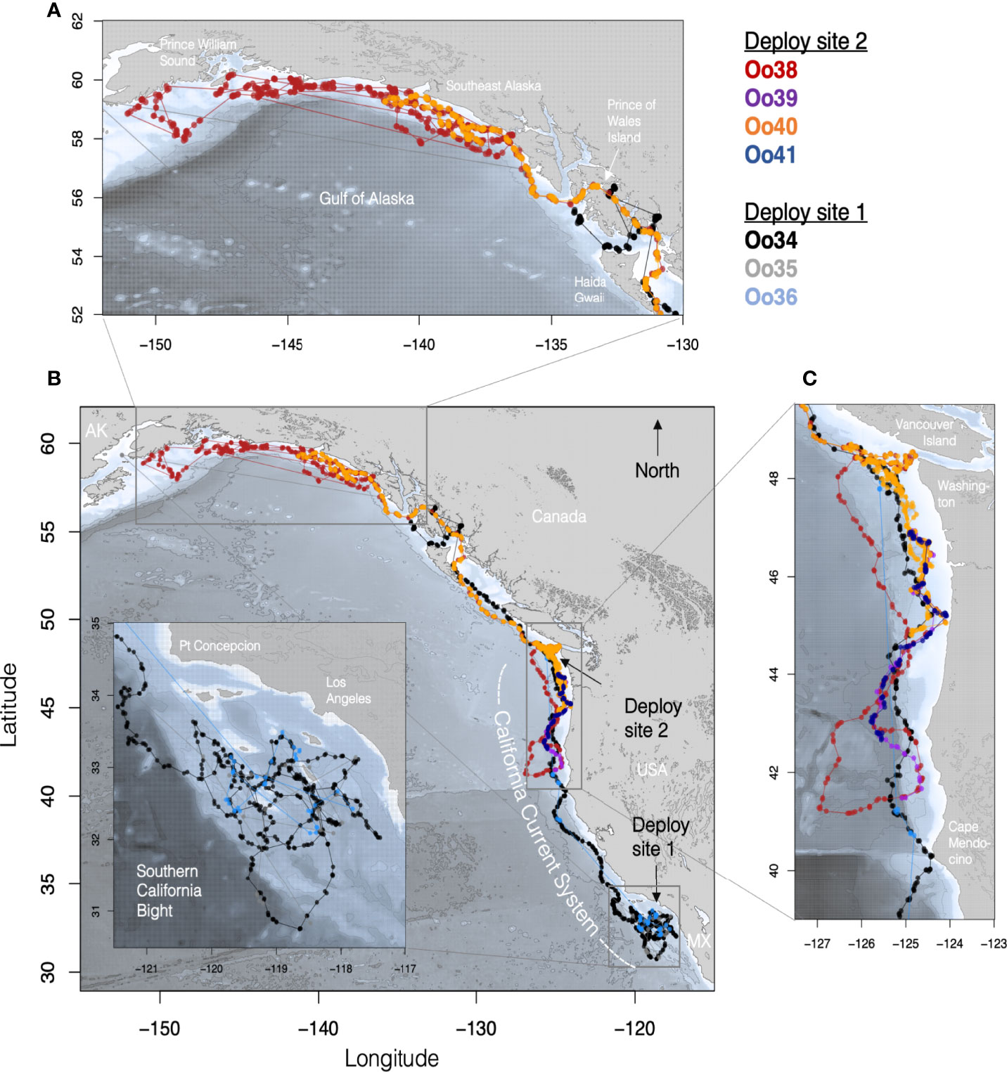
Figure 1 Maps of tagged Offshore killer whale tracks with each Offshore killer whale assigned a different color. (B) shows the complete set of filtered Argos tracks for animals tagged in both California (Deploy site 1) and Washington (Deploy site 2). (Inset) details of movements within the Southern California Bight, with the deployment site being just west of the southernmost island (San Clemente). (C) Tracks of whales from southern British Columbia to northern Oregon with the deployment site off the coast of WA indicated by the black arrow. (A) Track details of the movements within the Gulf of Alaska.

Sighting data including the time, location, group size, and primary behavior, for each group of cetaceans encountered were recorded using a custom database (Access, Microsoft Corporation, Redmond, WA). Photographs were collected of as many individuals encountered as possible and provided to curators of existing Offshore killer whale photo-ID catalogs for ecotype verification and individual identification (e.g. Black et al., 1997).

Two versions of the remotely deployed Low Impact Minimally Percutaneous External-electronics Transmitting (LIMPET) tag were used, both manufactured by Wildlife Computers, Inc. (Redmond, WA): the location-only SPOT5, and the location and dive reporting SPLASH10-A (Andrews et al., 2005; Schorr et al., 2014). Tag programming, including details on duty-cycling, are presented in Table 1. Tags were deployed using a Dan-Inject J.M. SP 25 pneumatic projector (Dan-Inject, ApS, Kolding, Denmark) at ranges of 4-16 m, and attached on or near the dorsal fin using two sterilized 6.7 cm long titanium darts with backwards facing ‘petals’ (Andrews et al., 2005). Reactions to tag deployments were recorded following Berrow et al. (2002), and information on the re-approachability of tagged whales was also documented to the best extent possible. Tag names were assigned according to a collaborative project naming scheme, including the Genus species code (Oo) followed by a sequential number code, regardless of ecotype. In this case, the first tag deployed on the group was the 34^th LIMPET tag deployed on a killer whale, and thus the deployment was named Oo34.

TABLE 1

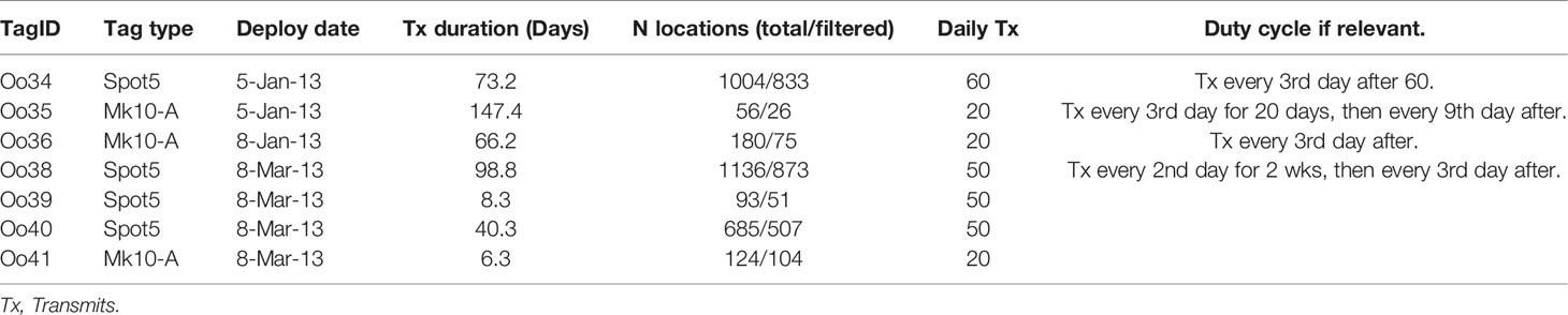
Table 1 Deployment details from Offshore killer whales tagged off California (Oo35 – Oo36) and Washington (Oo38 – Oo41), 2013.

Data Processing and Analysis

Argos location estimates were processed via the least-squared method (Argos User’s Manual, 2011), and subsequently filtered using the Douglas Argos Filter (Douglas et al., 2012). Filtering parameters were set as follows: a maximum sustainable rate of movement of 20 km/hr, retention of all location estimates class 2 and above, a maximum redundant distance setting of 3 km, and the filter default ratecoef of 25. One tag, Oo35, suffered an apparent malfunction that resulted in infrequent location estimates during the deployment, with only 31 location estimates generated during the 147.4 days the tag transmitted. No dive data was reported by the tag. Therefore, locations from this tag were only used to describe large-scale movements and not used in any of the detailed movement or dive analyses.

All subsequent analyses were conducted using the filtered datasets from the remaining tags. These included assessing overall minimum distance travelled, daily average minimum distance covered, distance between tagged whales, and an assessment of time spent in geographic regions. Geographic regions were defined by State (within the US) and Canada, with an additional region included for the SCB, which was defined as south of Point Conception (32.45°N). The California Current was defined as all locations south of 48.5°N. Geographic region was analyzed to assess variables that might change within management areas (e.g. U.S. versus British Columbia). Each location estimate was assigned its corresponding solar elevation, using the R package “maptools” (Bivand and Lewin-Koh, 2020; R Core Team, 2020). Water depth and distance from the 200 m isobath were calculated for each location estimate using the ETOPO1 dataset (1 arc-minute resolution) in ArcGIS v10.7.1 (NAD 1983 UTM Zone 11N) (Environmental Systems Research Institute (ESRI), 2019). To assess group stability over days, filtered location estimates received within 2 hours of each other were used to calculate distance between each tagged whale. When multiple locations were received within 2 hours in a single day, the smallest distance between qualifying location pairs was selected as the daily individual distance (typically a function of better location quality). Animals were presumed to be associated on a given day when individual distance was less than 20 km to allow for Argos error and movements during that period.

A geographic comparison of minimum rates of horizontal displacement and habitat use was conducted using the Douglas filtered location data, though locations less than 1 hour and greater than 6 hours apart were removed from the rate of displacement analysis to control for spurious rates (e.g. Baird et al., 2010). Locations were assigned to six latitudinal regions from Southern California to Alaska. The regions assessed were chosen to encompass management areas (U.S. versus Canada), then broken down either by other easily identifiable geographic boundaries such as State, or the SCB. Regions were, from South to North, SCB, Northern California, Oregon, Washington, British Columbia, and Alaska. The minimum rate of horizontal displacement and the distance to the 200 m bathymetric isobath were each modeled with generalized additive mixed models using the gamm4 package in R (Wood and Scheipl, 2020) as a function first of latitude (numeric) then of geographic region (categorical) with an additional categorical predictor for “TimeofDay” (day or night as a function of solar elevation) and nested random effects for “GroupID” (TagID, with a single TagID used when two whales were considered associated as defined above), “Day” (yyyymmdd), and HrCutoff (location grouping within 4 hr time blocks). These random effects were used to account for the autocorrelation between locations from the same animal (or group) on the same day and within hours of each other. The program was allowed to initially apply model smoothing algorithmically, and then the smoothing term was fixed manually to reduce overfitting of the data.

SPLASH10-A tags, which collected summarized dive data in the form of a Behavior Log (BL) in addition to Argos location estimates (Wildlife Computers, 2015), were deployed on three whales. One of these tags was Oo35, which did not report any dive data in addition to providing sparse location data due to its malfunction and was therefore excluded from dive analysis. BL collection days followed transmission duty cycling (Table 1). The parameters to define and record a dive differed slightly between the two remaining tags, based on lessons learned from the first deployment. Both tags were set to record the start/end of a dive using the wet/dry sensor. Oo36 recorded all dives that were longer than 30 sec and deeper than 20 m, while Oo41 recorded dives that were longer than 60 sec and deeper than 20 m. The increase in dive duration was implemented to reduce the number of ‘qualifying dives’ recorded, and to thus generate fewer BL messages to transmit each day, ideally resulting in a more contiguous dive record. Solar elevation was assigned to the start of each BL dive and surfacing by estimating the location of each event on an interpolated trackline between filtered location estimates, with solar elevations above -12 degrees considered day and the remaining locations assigned to night. Bottom depth was also calculated using the above methods at dive positions along the interpolated trackline to generate a rough assessment of dive depth compared to bottom depth. Given the limited sample size of individuals and somewhat lossy nature of telemetered data, it was neither feasible nor appropriate to quantify correlations among dive behavior and additional environmental factors, and only observational assessments were made.

Results

Deployment Summary

Offshores were encountered during three small vessel surveys in 2013. The first and second encounters were in the outer waters of the SCB in January during marine mammal surveys at SOAR. The first encounter was with a group of six individuals on January 5^thand was facilitated by acoustic direction from the M3R system (Moretti et al., 2010, Jarvis et al., 2014). Acoustic recordings were made of the hydrophones nearest the visually-verified encounter, and later comparison showed the structure of the calls to match published vocalizations of the ecotype (Filatova et al., 2012). Two tags were deployed during this encounter, one on an adult male (Oo34) and one on a subadult of unknown sex (Oo35). The second encounter occurred on January 8^th and was facilitated by using locations from the two whales tagged during the first encounter. This group was estimated as nine individuals including both previously tagged whales, as well as at least two other individuals identified during the encounter on the 5^th. An adult male, who was present during the encounter on the 5^th, was tagged (Oo36). The third encounter with Offshores occurred near Grays Harbor Canyon off the outer coast of Washington on March 8^th, during a joint survey with the Northwest Fisheries Science Center cruise for Southern Resident Killer whales, and was not associated with any of the previously tagged whales. This group was estimated at 30 individuals. Four tags were deployed during the encounter (Oo38-41), three on presumed adult females and one on an adult male based on morphology.

Tags transmitted data across an average of 62.9 days (median = 66.2, min = 6.3, max = 147.4, Table 1). The shortest transmission durations were associated with suboptimal tag placements: one tag was attached just below the dorsal fin and transmitted only 8.3 days, and one tag was attached at the trailing edge of the fin via a single dart and lasted 6.3 days. Reactions to tagging were classified as either “none” (n = 1) or “moderate” (n = 6), the latter of which consisted primarily of a tail flick with acceleration or a roll (Berrow et al., 2002). Four of the whales were reapproached to within 20 m within 45 min of tagging. None of the individuals demonstrated apparent avoidance behavior and two animals actively reapproached to within 4 m of the vessel after tagging, including swimming directly astern of the vessel while underway.

Movements and Habitat Use

Oo34 and Oo36 spent the first 34 days of their deployment associated together and circling broadly within the SCB, with coincident location estimates during this period an average of 10 km apart (sd = 13.0, n = 25), though after the first 20 days tag Oo36 was duty cycled to transmit every 3^rd day, reducing the number of coincident locations for the two whales during the latter part of the period. During this time, the whales spent most of their time in the outer waters of the SCB, never coming closer than 30 km of the mainland (Figure 1B). Thirty-four days after the first tag deployment, both whales moved out of the SCB, passing north of Point Conception with coincident Argos location estimates within 1 km of each other (Figure 1A). Oo35 transmitted infrequently, but the few locations received from the tag were near locations from the other two whales for the first 19 days of the deployment (range = 0.8 – 14.5 km, n = 8). The next location estimate from Oo35 was not received until 75 days later, when two locations were received in Prince William Sound, AK, more than 3,800 km from the tagging location (Figures 1A, D).

Oo34 and Oo36 appeared to travel together to the northern tip of Washington (48.1°N), and 52 days after tagging (February 26^th), individual daily locations were within 3 km, more than 1,634 km away from where they were tagged. Oo36 then turned south, doubling back at least as far as southern Oregon (43.3°N) before the tag stopped transmitting. Meanwhile Oo34 continued travelling north, turning east into more inland waters upon reaching the south end of Haida Gwaii, British Columbia, then into the inner waters of Southeast Alaska (SEAK) (Figure 1A). By the 61^st day (March 7^th) after Oo34 was tagged, and the last day with concurrent locations, Oo34 and Oo36 were a straight-line distance of 1,339 km apart (Figure 1B). Ultimately, Oo34 travelled north through the inner waters of SEAK nearly to Wrangell, reaching a maximum of just over 2,800 km from the tagging location before heading west to the outer waters of SEAK, where the tag stopped transmitting.

When the next four tags were deployed on the other group of Offshores on March 8^th, Oo34 was more than 1,000 km to the north and Oo36 was more than 400 km to the south of the location where these whales were tagged off the coast of Washington, based on locations received the previous day. The whales tagged off Washington remained associated for four days post-tagging while moving south, at which point Oo40 separated and turned back north. The maximum separation between Oo40 and the other three whales reached 730 km by the 6^th day after tagging. The remaining three whales stayed together until Oo39 and Oo41 stopped transmitting (Figure 1C), travelling as far south as northern California. On March 16^th, locations received from duty-cycled tag Oo36 indicate that the then northbound whales tagged in California likely passed the whales tagged off Washington somewhere off the coast of Oregon or Washington, with Oo36 now 100 km north of Oo40 and 550 km north of Oo38 and Oo39.

The grand mean of point-to-point horizontal movement rates (n = 672) averaged 3.5 km/hr (individual range 0.1 – 14.5 km/hr) (Table 2) throughout the deployment period. Model results of horizontal displacement rates as a function of latitude revealed no change in speed by latitude (F = 0.0, df =9, p = 1.0);.

TABLE 2

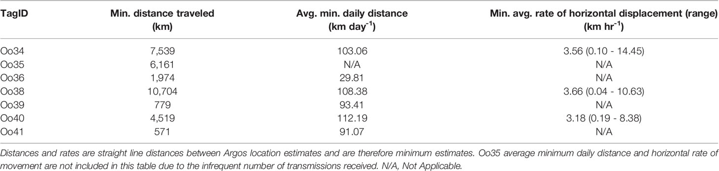
Table 2 Movement details.

Of the tags deployed in the SCB, Oo34 had the most complete location record, and was considered representative of regional habitat use by the whales that were tagged together in the region. The whale appeared to preferentially travel along the many submarine banks and ridges in the area, versus spending time in the center of the deep basins they surround. However, Oo34 used significantly deeper habitat in the SCB than he did in the northern extent of the California Current (median = 1,182 m versus 642 m, Kruskal-Wallis One-way ANOVA z-value = 6.97, p < 0.0001). As he, and the other tagged whales that were associated with him, moved up the coast through central and northern California, Oregon, and Washington, the whales spent nearly all their time along the continental slope, with most locations deeper than the 200 m isobath (Figure 1). Towards the northern end of the California Current, the whales shifted their distribution closer to the 200 m isobath, and within BC and Alaska the whales increasingly used waters shallower than 200 m (Figure 2).

FIGURE 2

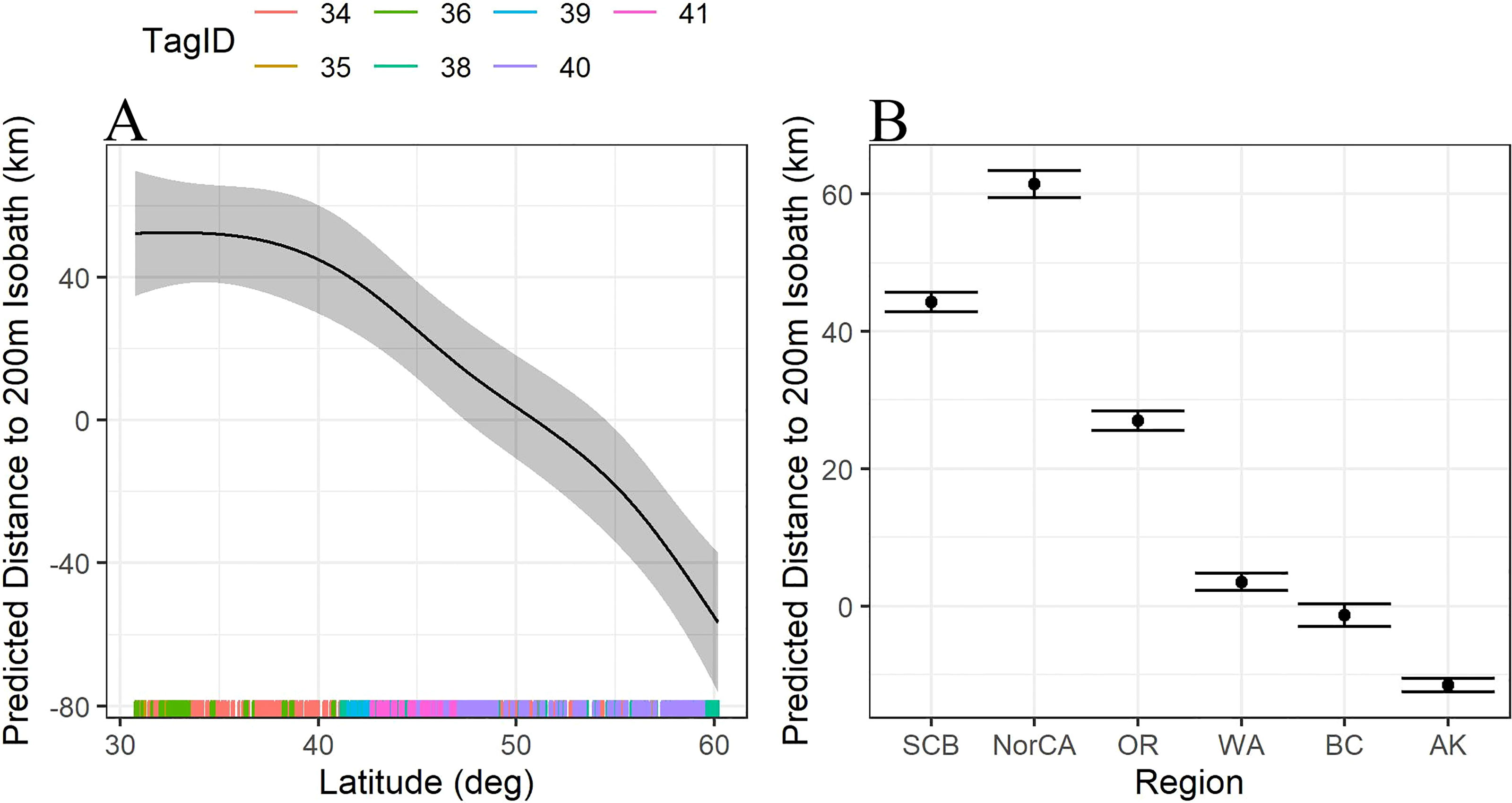
Figure 2 (A) Trendline for the predicted distance to the 200m isobath (km) as a function of latitude. Distances below 0 are shallower than 200m, distances greater than 0 are deeper than 200m. (B) Predicted distance to the 200m isobath (km) as a function of region. Habitat use south of WA are much further offshore, habitat use north of WA is generally up on the shelf edge, inside the 200m isobath. SCB=Southern California Bight including all locations south of Pt Conception (n=476); NorCA = Northern California, including all latitudes north of Pt Conception to Oregon State boundary (n=188); OR, Oregon (n=377); WA, Washington (n=447); BC, British Columbia (n=253); AK, Alaska (n=728).

By March 23^rd, both Oo38 and Oo40 (now the only two tags deployed off Washington still transmitting) were using the waters off the coast of WA, but Oo38 was at the bottom of the continental slope while Oo40 was utilizing waters over the top of the continental shelf (Figure 1). Seventeen days after deployment, and 13 days after separating, the two whales reunited at the shelf edge. In the next 24 days that both tags transmitted, the mean distance between assessed daily locations was 0.5 km (max = 5.9, n=25), as they traveled through BC, around Prince of Wales Island in SEAK, then west along the outer continental shelf, reaching as far as 1,720 km away from the tagging location before Oo40 stopped transmitting. Oo38 continued to move along the Pacific coast of Alaska, reaching as far north and west as the islands outside of Prince William Sound. While most of the time was spent along the shelf edge, the whale also spent time in deep water beyond the shelf break and in near-shore waters (Figure 1).

Latitude significantly predicted the distance to the 200 m isobath (F = 0.9, df = 4, p = 0.0004), with whales furthest from shore at latitudes around 30°N, generally approaching the 200 m isobath at latitudes near 50°N, then transitioning to habitat inside the 200 m isobath at latitudes further north (Figure 2A). Similarly, habitat use varied significantly by region, with locations off California and Oregon significantly deeper than the 200 m isobath than those off Washington, British Columbia, and Alaska (Figure 2B).

Dive Behavior

Two deployments (Oo36 from California and Oo41 from Washington) were SPLASH10-A tags that recorded depth and duration of qualifying dives (Figures 3A–E) and duration of the surface intervals between them (Table 3). Oo36 transmitted 500 dives (qualifying dives are defined as submergences deeper than 20 m lasting at least 30 sec) and surface intervals over 66.2 days of transmission while it moved north along the California coast up into the northern end of Washington. Oo36’s median dive depth was 41 m (max = 479.5), median dive duration was 3.9 min (Max = 10.1), and median surface interval was 3.7 minutes. The maximum time between qualifying dives during periods of continuous dive data collection was 618 minutes (10.3 hours). Oo41 transmitted 610 dives (submergences greater than 20 m lasting at least 60 sec) and corresponding surface intervals over 6.3 days of transmission while it moved south from Washington to northern California (Figure 4). Its median dive depth was 99.5 m (max = 479.5), median dive duration was 4.1 min (max = 12.3 min), and median surface interval was 2.5 minutes (max = 595). No dive data was recorded within B.C. or Alaska.

FIGURE 3

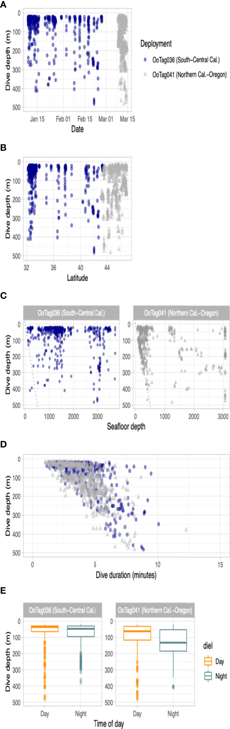
Figure 3 Parameters of dive data recorded by the two whales tagged with SPLASH10-A dive reporting LIMPET tags. Dive activity is plotted by (A) dive depth versus date; (B) dive depth versus latitude; (C) dive depth versus seafloor depth; (D) dive depth versus dive duration and; (E) dive depth by time of day. In the scatter plots, blue circles are data from Oo36 and gray triangles are data from Oo41.

TABLE 3

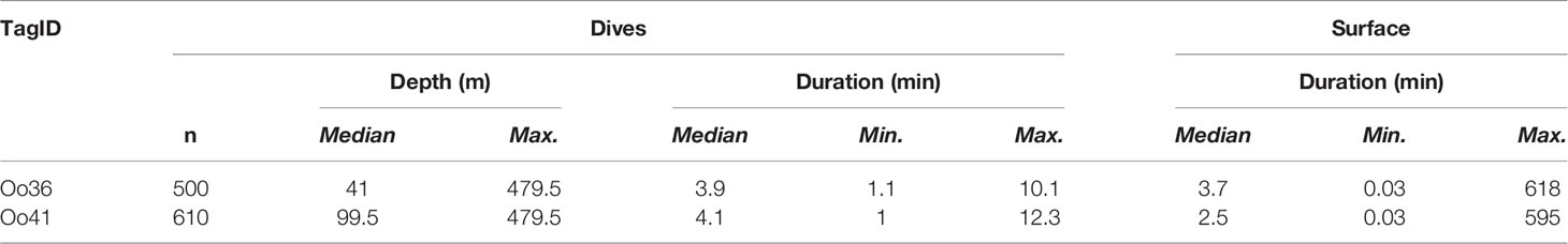
Table 3 Dive and surfacing summary of the two SPLASH10-A tagged whales that reported data.

FIGURE 4

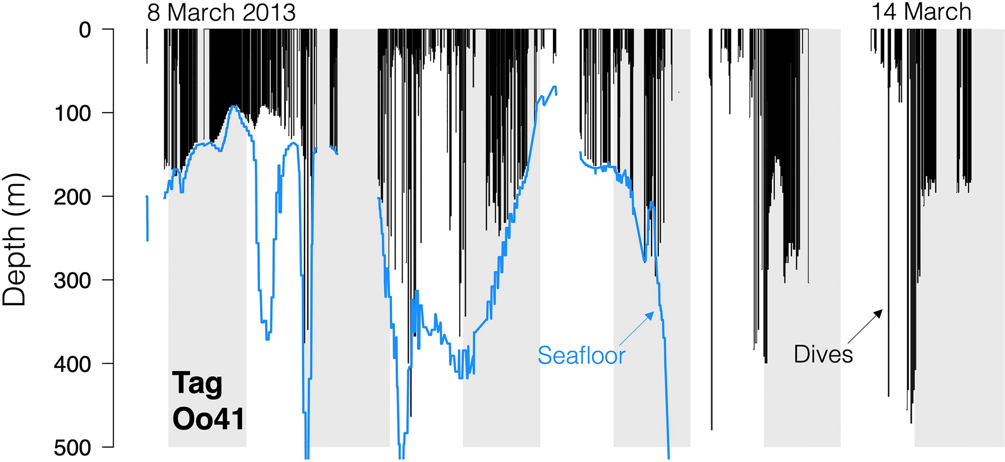
Figure 4 Dive traces for Tag Oo41 (March 2013, off northern California and Oregon and Washington, USA). Black bars are the dives, with line discontinuities representing periods where no dive data was received. Blue line is the local seafloor depth.

No strong diel patterns were evident in a visual exploration of the dive record, (Figure 3E and 5); however more dives were recorded during daylight hours (59.0%)), as were most of the deeper dives (>300m). Dive data from Oo41 revealed the following patterns of association with the seafloor depth: in regions where bottom depths were shallower than 450 m, this whale frequently appeared to dive to or near the seafloor (Figure 4). These dives to seafloor depth happened primarily during nighttime, though this may have been coincidental. In waters deeper than 450 m, dive depth did not appear correlated with seafloor depth and shallower dives were regularly executed to midwater depths (100 – 300 m), with the deepest dives occurring during the day.

FIGURE 5

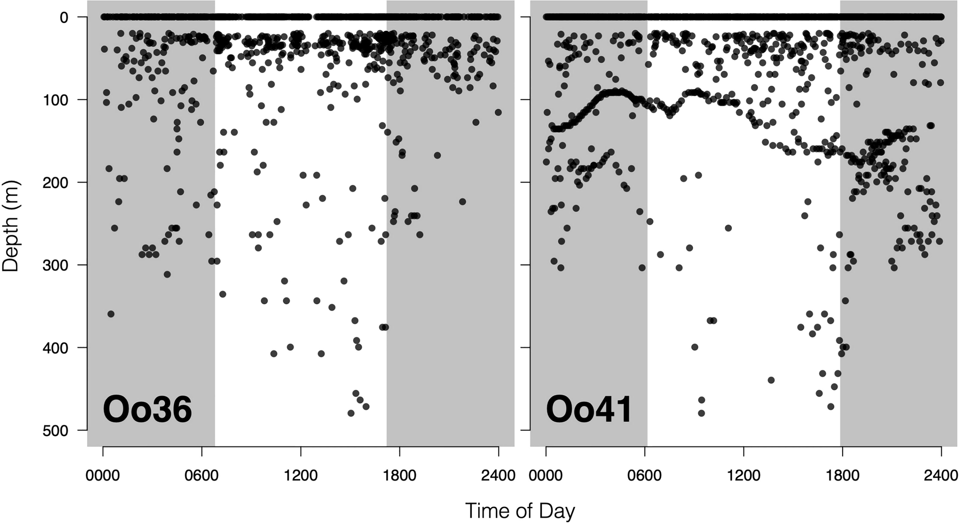
Figure 5 Offshore killer whale dive activity plotted as function of time of day. Shaded areas are periods of dark, defined by the mean sunrise time and mean sunset time during the deployment. The lack of activity between 1 and 20 meters is a function of tag programming, which considers all dives shallower than 20m as ‘surface’ time. The striking undulating pattern in dive depths for Tag Oo41 is likely a response to local seafloor depth.

Discussion

Movements and Habitat Use

Offshores are known to travel more extensively than other ecotypes of the northeast Pacific based on photo-ID records (Dahlheim et al., 2008; Ford et al., 2014). The extent and rates of movements observed with these tags, which included individuals using nearly the entirety of the population’s known range within the transmission period, generally corresponded with the photograph-based movements documented in previous studies (Dahlheim et al., 2008; Ford et al., 2014), though they expand the known range of this ecotype further south than has been previously documented through sightings and adds substantial detail on their movement patterns during the period of tag transmission. While movements across the entire range within a single year have been documented photographically (Dahlheim et al., 2008), the tag data demonstrates that whales move these distances in less than three months. Four whales were documented travelling at least 4,000 km and covering at least 100 km per day, increasing the previous best estimate of Offshore travel rates by two-to threefold (Dahlheim et al., 2008). The whale with one of the longest transmitting tags, Oo38, traveled at least 10,704 km in 99 days. These daily travel rates are comparable to those documented for killer whales elsewhere in the world, including the Southern Ocean (up to 223 km/day, n = 6; Durban and Pitman, 2012) and the North Atlantic (96.1 -159.6 km/day, n =1; Matthews et al., 2011). Both the broad-scale movement patterns and the finer-scale movement rates captured by these tags between January and June are consistent with the hypothesis that Offshores engage in a diffuse northward shift in habitat use in the first half of the year (Ford and Ellis, 2014; Ford et al., 2014), though animals were present in Alaskan waters earlier in the year than has been previously documented. All five individuals with transmission durations greater than one month traveled to higher latitudes during their deployments. Four of these whales tagged off the US West Coast in winter arrived in Alaskan waters and remained there for weeks before their tags ceased transmitting. For example, Oo38 remained in Alaskan waters from its arrival in early April until the end of tag transmission in mid-June. To date, Offshores have been encountered in Alaskan waters primarily during surveys in summer and early fall (Zerbini et al., 2007; Dahlheim et al., 2008; Dahlheim et al., 2009). Oo34 arrived in SEAK by early March, and Oo35 and 40 were both in SEAK by early April. All of these whales remained in the waters of Alaska and northern B.C. throughout the spring, including time within nearshore passages and inlets. These findings corroborate the suggestions that existing data, which are seasonally biased, underrepresent the importance of Alaskan waters during spring (e.g. Dahlheim et al., 2008; Ford et al., 2014). These data also suggest the importance of habitat along the US West Coast and northern Mexico in winter has been previously underrepresented by the limited sightings from the region.

As part of this seasonal shift in their range, these tagged Offshores also appear to alter their preferred habitat, gradually shifting into shallower water as they move north in the spring (Figure 2). Offshores generally preferred deeper habitat beyond the shelf break along the US West Coast, which has likely contributed to low detection rates in this part of their range. One notable deviation from this pattern in these data occurred off Cape Mendocino, CA (latitude ~40.35°N), where locations were received as close as 3.2 km from the coast. While this shift may have been habitat-associated, a deep canyon comes very near shore in this area, coincidentally, a concurrently tagged Southern Resident killer whale (SRKW, K25) was also present in the nearshore waters of Cape Mendocino at the same time (Hanson et al., unpublished data). Multiple Argos location estimates were received from both ecotypes within a 12-hour period, the closest of which was 2.0 km and 2 hours apart. By itself, this event may have been unremarkable. However, the larger group of Offshores that was encountered and tagged off WA in March was initially sighted by a NOAA survey vessel that had acoustically tracked a group of SRKW to the shelf break, an unusual movement away from the coastal waters that represent their typical range (Hanson et al., 2017; Rice et al., 2017). These two anecdotal events taken together suggest that these two ecotypes may occasionally leave preferred habitat to spatially associate, at least briefly. Though there is no evidence of recent gene flow among sampled Offshore and Resident ecotypes, the two are more closely related to each other than they are to sympatric Transient killer whales (Morin et al., 2006).

Using photo-identified individuals from different encounters of Offshore killer whales, Ford et al. (2014) assessed social organization within the ecotype using a pair-wise association approach. While the results suggested some possible stable groupings of individuals, the results were clear that the social structure of Offshores is not as strong as that of sympatric Resident and Transient ecotypes, with only some individuals showing recurrent associations over multiple encounters. Persistent bonds lasting more than a decade have been observed between Offshore adult females and males, but not between reproductive females, as are seen in the multi-generational matrilines of Residents (Ford and Ellis, 2014).

Though some whales tagged in the same group remained associated for as long as 52 days, all individuals whose tags transmitted more than nine days ultimately separated from each other. This was true even for the whales tagged together in a relatively small group of nine. While apart, some whales tagged together moved along similar routes, just with the timing offset from one another (Figure 1). For example, O34 and Oo36 appeared to travel up the west coast of the US, before parting ways. Oo35 began with this same group but was present in Prince William Sound at the same time as whales tagged in WA were travelling south into CA. Oo38 and Oo40 traveled north along similar routes with their paths only crossing periodically, such as when they passed off the southern tip of Haida Gwaii on the same day. Taken together, the movements we observed support prior observations that the social structure of Offshores is more fluid than that of other ecotypes (Ford et al., 2014), and includes some persistent and recurrent associations that may occur over long distances as whales use similar seasonal travel routes.

Dive Behavior

Though the sample size is small, this is the first study to report dive data from Offshore killer whales. The dive patterns of these tagged whales indicate that Offshores may use the water column broadly while foraging, including the seafloor in certain locations (Figure 3C and Figure 5). Several known prey species of Offshores are associated with the seafloor; these include the Pacific sleeper shark (Ford et al., 2014), spiny dogfish, and Pacific halibut (Fisheries and Oceans Canada, 2018). Sleeper sharks are also known to occupy both demersal and pelagic habitats at a wide range of depths (Hulbert et al., 2006), and this broad availability may explain the apparent importance of this prey species to Offshores (Ford et al., 2014). The remaining species of known prey, including blue sharks, Pacific salmon, and opah, are also wide-ranging inhabitants of epipelagic to mesopelagic waters (e.g. Polovina et al., 2008; Markaida and Sosa-Nishizaki, 2010; Wright et al., 2017). The wide range of vertical habitat used by these whales, coupled with their extensive movements, supports the hypothesis that Offshores can respond flexibly to prey availabilities that vary by region, season, and seafloor depth.

Many dives in this dataset were deep relative to those described from other sympatric ecotypes in the northeast Pacific. Previous dive records from this region include a maximum of 254 m for Transient killer whales (Miller et al., 2010), 379 m for Northern Resident killer whales (Wright et al., 2017), and a maximum of 300 m for whales in the SRKW population (Tennessen et al., 2019). Dive depths recorded here were more similar to those seen in killer whales of the Southern Ocean, which regularly dive deeper than 350 m (maximum = 767.5 m), presumably to forage upon vertically migrating cephalopods and the demersal Patagonian toothfish (Dissostichus eleginoides) (Reisinger et al., 2015).

Conclusions

Here we present the first telemetry data on the movements, habitat use, and dive behavior of Offshore killer whales in the northeast Pacific. Many of our findings are consistent with inferences from photograph-based research over the last three decades (e.g Ford et al., 2014), including that Offshores undertake seasonal latitudinal shifts. These data provide valuable insights into how individual Offshore killer whales move throughout their expansive range, covering remarkable distances in periods of less than three months, and suggest they are relative ecological generalists among the other, more specialized, northeast Pacific killer whale ecotypes thus described. This detailed and relatively unbiased look at habitat use can inform management decisions in US waters and beyond.

Data Availability Statement

The raw data supporting the conclusions of this article will be made available by the authors, without undue reservation.

Ethics Statement

All methods and protocols were reviewed by the NMFS permit office, and all work was conducted under NOAA Research Permits, No.’s 16111 and 16163. Tagging conducted under Cascadia Research Collective IACUC protocol number CRC-2011-AUP-01-03.

Author Contributions

GS, EF, and SJ conducted the field work in CA. GS, EF, MH, and CE led the field work in WA. GS and EK conducted the data analysis. RA led the development of the LIMPET tags. All authors contributed to the generation of the manuscript. All authors contributed to the article and approved the submitted version.

Funding

Funding for field work and tags deployed in California were provided by funding from the Chief of Naval Operations Environmental Readiness Division (N45) via a grant from the Naval Postgraduate School (Grant No. N000244-10-1-0050). Funding for field work and tags deployed in WA came from the Northwest Fisheries Science Center, and from the U.S. Navy, Pacific Fleet (via a contract to Cascadia Research Collective from HDR, No. N62470-10-D-3011).

Conflict of Interest

The authors declare that the research was conducted in the absence of any commercial or financial relationships that could be construed as a potential conflict of interest.

Publisher’s Note

All claims expressed in this article are solely those of the authors and do not necessarily represent those of their affiliated organizations, or those of the publisher, the editors and the reviewers. Any product that may be evaluated in this article, or claim that may be made by its manufacturer, is not guaranteed or endorsed by the publisher.

Acknowledgments

We would like to thank individuals involved in the field support for this work, including Dave Moretti, Jeff Foster, Brenda Rone, and Frank and Jane Falcone. We thank Alisa Schulman-Janiger for confirmation of whales tagged in CA as Offshore killer whales. We are grateful to the officers, crew, and science teams on the Bell M. Shimada in the 2013 PODs cruise for their assistance with the Offshores encounter. Additional support for analysis and review was provided by Brenda Rone, David Sweeney and Shannon Coates. We also thank the three reviewers for their comments and suggestions in improving the manuscript. Tagging was conducted under NOAA research permits 16111 issued to Cascadia Research Collective, and 16163 issued to the Northwest Fisheries Science Center.

References

Andrews R. D., Mazzuca L., Matkin C. O. (2005). Satellite Tracking of Killer Whales In: Synopsis of Research on Steller Sea Lions: 2001 – 2005. Eds. Loughlin T. R., Atkinson S., Calkins D. G. (Alaska SeaLife Center Seward, AK: Alaska SeaLife Center).

Google Scholar

Baird R., Schorr G., Webster D., McSweeney D., Hanson M., Andrews R. (2010). Movements and Habitat Use of Satellite-Tagged False Killer Whales Around the Main Hawaiian Islands. Endangered Species Res. 10, 107–121. doi: 10.3354/esr00258

CrossRef Full Text | Google Scholar

Berrow S. D., McHugh B., Glynn D., McGovern E., Parsons K. M., Baird R. W., et al. (2002). Organochlorine Concentrations in Resident Bottlenose Dolphins (Tursiops Truncatus) in the Shannon Estuary, Ireland. Marine Pollution Bull. 44, 1296–1303. doi: 10.1016/S0025-326X(02)00215-1

CrossRef Full Text | Google Scholar

Bivand R., Lewin-Koh N. (2020). “Maptools,” in Tools for Handling Spatial Objects.

Google Scholar

Black N., Schulman-Janiger A., Ternullo R., Guerrero-Ruiz M. (1997). Killer Whales of California and Western Mexico (La Jolla, CA: National Marine Fisheries Service).

Google Scholar

Collecte Localisation Satellite. (2011). Argos User’s Manual.

Google Scholar

Dahlheim M. E., Schulman-Janiger A., Black N., Ternullo R., Ellifrit D., Balcomb K. I. I. I. (2008). Eastern Temperate North Pacific Offshore Killer Whales (Orcinus Orca): Occurrence, Movements, and Insights Into Feeding Ecology. Marine Mammal Sci. 24, 11. doi: 10.1111/j.1748-7692.2008.00206.x

CrossRef Full Text | Google Scholar

Dahlheim M. E., White P. A., Waite J. M. (2009). Cetaceans of Southeast Alaska: Distribution and Seasonal Occurrence. J. Biogeogr. 36, 410–426. doi: 10.1111/j.1365-2699.2008.02007.x

CrossRef Full Text | Google Scholar

Douglas D. C., Weinzierl R., Davidson S. C., Kays R., Wikelski M., Bohrer G. (2012). Moderating Argos Location Errors in Animal Tracking Data. Methods Ecol. Evol. 3, 999–1007. doi: 10.1111/j.2041-210X.2012.00245.x

CrossRef Full Text | Google Scholar

Durban J. W., Pitman R. L. (2012). Antarctic Killer Whales Make Rapid, Round-Trip Movements to Subtropical Waters: Evidence for Physiological Maintenance Migrations? Biol. Lett. 8, 274–277. doi: 10.1098/rsbl.2011.0875

PubMed Abstract | CrossRef Full Text | Google Scholar

Filatova O. A., Deecke V. B., Ford J. K. B., Matkin C. O., Barrett-Lennard L. G., Guzeev M. A., et al. (2012). Call Diversity in the North Pacific Killer Whale Populations: Implications for Dialect Evolution and Population History. Anim. Behav. 83, 595–603. doi: 10.1016/j.anbehav.2011.12.013

CrossRef Full Text | Google Scholar

Fisheries and Oceans Canada. (2018). Recovery Strategy for the Offshore Killer Whale (Orcinus Orca) in Canada (Ottawa: Fishereis and Oceans Canada). Available at: http://publications.gc.ca/collections/collection_2018/eccc/En3-4-293-2018-eng.pdf (Accessed April 13, 2021).

Google Scholar

Ford J. K., Ellis G. M. (2014). “You are What You Eat: Foraging Specializations and Their Influence on the Social Organization and Behavior of Killer Whales,” in Primates and Cetaceans (Japan: Springer), 75–98.

Google Scholar

Ford J., Ellis G., Balcomb K. (2000). “Killer Whales,” in The Natural History and Genealogy of Orcinus Orca in British Columbia and Washington State. Vancouver (British Columbia: UBC Press).

Google Scholar

Ford J., Ellis G., Matkin C., Wetklo M., Barrett-Lennard L., Withler R. (2011). Shark Predation and Tooth Wear in a Population of Northeastern Pacific Killer Whales. Aquat. Biol. 11, 213–224. doi: 10.3354/ab00307

CrossRef Full Text | Google Scholar

Ford J. K. B., Stredulinsky E. H., Ellis G. M., Durban J. W., Pilkington J. F. (2014). “Offshore Killer Whales in Canadian Pacific Waters,” in Distribution, Seasonality, Foraging Ecology, Population Status and Potential for Recovery (Ottawa, Ontario: DFP Canada Science Advisory Secretariat).

Google Scholar

Hanson M. B., Ward E. J., Emmons C. K., Holt M. M. (2017). Modeling the Occurrence of Endangered Killer Whales Near a U.S. Navy Training Range in Washington State Using Satellite-Tag Locations to Improve Acoustic Detection Data (Seattle, WA: NOAA, Northwest Fisheries Science Center), Vol. 41.

Google Scholar

Heise K., Barrett-Lennard L. G., Saulitis E., Matkin C., Bain D. (2003). Examining the Evidence for Killer Whale Predation on Steller Sea Lions in British Columbia and Alaska. Aquat. Mammals 29, 325–334. doi: 10.1578/01675420360736497

CrossRef Full Text | Google Scholar

Herman D., Burrows D., Wade P., Durban J., Matkin C., LeDuc R., et al. (2005). Feeding Ecology of Eastern North Pacific Killer Whales Orcinus Orca From Fatty Acid, Stable Isotope, and Organochlorine Analyses of Blubber Biopsies. Mar. Ecol. Prog. Ser. 302, 275–291. doi: 10.3354/meps302275

CrossRef Full Text | Google Scholar

Hulbert L. B., Sigler M. F., Lunsford C. R. (2006). Depth and Movement Behaviour of the Pacific Sleeper Shark in the North-East Pacific Ocean. J. Fish Biol. 69, 406–425. doi: 10.1111/j.1095-8649.2006.01175.x

CrossRef Full Text | Google Scholar

Jarvis S. M., Morrissey R. P., Moretti D. J., DiMarzio N. A., Shaffer J. A. (2014). Marine Mammal Monitoring on Navy Ranges (M3R): A Toolset for Automated Detection, Localization, and Monitoring of Marine Mammals in Open Ocean Environments. Marine Technol. Soc. J. 48, 5–20. doi: 10.4031/MTSJ.48.1.1

CrossRef Full Text | Google Scholar

Jones I. M. (2006). A Northeast Pacific Offshore Killer Whale (Orcinus Orca) Feeding On A Pacific Halibut (Hippoglossus Stenolepis). Marine Mammal Sci. 22, 198–200. doi: 10.1111/j.1748-7692.2006.00013.x

CrossRef Full Text | Google Scholar

Krahn M. M., Herman D. P., Matkin C. O., Durban J. W., Barrett-Lennard L., Burrows D. G., et al. (2007). Use of Chemical Tracers in Assessing the Diet and Foraging Regions of Eastern North Pacific Killer Whales. Marine Environ. Res. 63, 91–114. doi: 10.1016/j.marenvres.2006.07.002

CrossRef Full Text | Google Scholar

Markaida U., Sosa-Nishizaki O. (2010). Food and Feeding Habits of the Blue Shark Prionace Glauca Caught Off Ensenada, Baja California, Mexico, With a Review on its Feeding. J. Marine Biol. Assoc. United Kingdom 90, 977–994. doi: 10.1017/S0025315409991597

CrossRef Full Text | Google Scholar

Matthews C. J. D., Luque S. P., Petersen S. D., Andrews R. D., Ferguson S. H. (2011). Satellite Tracking of a Killer Whale (Orcinus Orca) in the Eastern Canadian Arctic Documents Ice Avoidance and Rapid, Long-Distance Movement Into the North Atlantic. Polar Biol. 34, 1091–1096. doi: 10.1007/s00300-010-0958-x

CrossRef Full Text | Google Scholar

Miller P. J. O., Shapiro A. D., Deecke V. B. (2010). The Diving Behaviour of Mammal-Eating Killer Whales (Orcinus Orca): Variations With Ecological Not Physiological Factors. Can. J. Zoology 88, 1103–1112. doi: 10.1139/Z10-080

CrossRef Full Text | Google Scholar

Moretti D., Marques T. A., Thomas L., DiMarzio N., Dilley A., Morrissey R., et al. (2010). A Dive Counting Density Estimation Method for Blainville’s Beaked Whale (Mesoplodon Densirostris) Using a Bottom-Mounted Hydrophone Field as Applied to a Mid-Frequency Active (MFA) Sonar Operation. Appl. Acoustics 71, 1036–1042. doi: 10.1016/j.apacoust.2010.04.011

CrossRef Full Text | Google Scholar

Moretti D., Morrissey R., DiMarzio N., Ward J. (2006). Verified Passive Acoustic Detection of Beaked Whales (Mesoplodon Densirostris) Using Distributed Bottom-Mounted Hydrophones in the Tongue of the Ocean, Bahamas. J. Acoustical Soc. America 119, 3374. doi: 10.1121/1.4786579

CrossRef Full Text | Google Scholar

Morin P. A., LeDuc R. G., Robertson K. M., Hedrick N. M., Perrin W. F., Etnier M., et al. (2006). Genetic Analysis of Killer Whale (Orcinus Orca) Historical Bone and Tooth Samples to Identify Western U.s. Ecotypes. Mar. Mammal Sci. 22, 897–909. doi: 10.1111/j.1748-7692.2006.00070.x

CrossRef Full Text | Google Scholar

Polovina J. J., Hawn D., Abecassis M. (2008). Vertical Movement and Habitat of Opah (Lampris Guttatus) in the Central North Pacific Recorded With Pop-Up Archival Tags. Marine Biol. 153, 257–267. doi: 10.1007/s00227-007-0801-2

CrossRef Full Text | Google Scholar

R Core Team. (2020). “R: A Language and Environment for Statistical Computing,” in R Foundation for Statistical Computing (Vienna, Austria: R Foundation for Statistical Computing). Available at: https://www.R-project.org/.

Google Scholar

Reisinger R. R., Keith M., Andrews R. D., de Bruyn P. J. N. (2015). Movement and Diving of Killer Whales (Orcinus Orca) at a Southern Ocean Archipelago. J. Exp. Mar. Biol. Ecol. 473, 90–102. doi: 10.1016/j.jembe.2015.08.008

CrossRef Full Text | Google Scholar

Rice A., Deecke V., Ford J., Pilkington J., Oleson E., Hildebrand J., et al. (2017). Spatial and Temporal Occurrence of Killer Whale Ecotypes Off the Outer Coast of Washington State, USA. Mar. Ecol. Prog. Ser. 572, 255–268. doi: 10.3354/meps12158

CrossRef Full Text | Google Scholar

Schorr G. S., Falcone E. A., Moretti D. J., Andrews R. D. (2014). First Long-Term Behavioral Records From Cuvier’s Beaked Whales (Ziphius Cavirostris) Reveal Record-Breaking Dives. PloS One 9, e92633. doi: 10.1371/journal.pone.0092633

PubMed Abstract | CrossRef Full Text | Google Scholar

Tennessen J. B., Holt M. M., Ward E. J., Hanson M. B., Emmons C. K., Giles D. A., et al. (2019). Hidden Markov Models Reveal Temporal Patterns and Sex Differences in Killer Whale Behavior. Sci. Rep. 9, 14951. doi: 10.1038/s41598-019-50942-2

PubMed Abstract | CrossRef Full Text | Google Scholar

Wildlife Computers. (2015). Wildlife Computers Splash10 Tag and Host User Guide. Available at: http://wildlifecomputers.com/downloads.aspx.

Google Scholar

Wood S., Scheipl F. (2020). “Gamm4,” in Generalized Additive Mixed Models Using “Mgcv” and “Lme4”. Available at: https://CRAN.R-project.org/package=gamm4.

Google Scholar

Wright B. M., Ford J. K. B., Ellis G. M., Deecke V. B., Shapiro A. D., Battaile B. C., et al. (2017). Fine-Scale Foraging Movements by Fish-Eating Killer Whales (Orcinus Orca) Relate to the Vertical Distributions and Escape Responses of Salmonid Prey (Oncorhynchus Spp.). Mov. Ecol. 5, 3. doi: 10.1186/s40462-017-0094-0

PubMed Abstract | CrossRef Full Text | Google Scholar

Zerbini A. N., Waite J. M., Durban J. W., LeDuc R., Dahlheim M. E., Wade P. R. (2007). Estimating Abundance of Killer Whales in the Nearshore Waters of the Gulf of Alaska Adn Aleutian Islands Using Line-Transect Sampling. Mar. Biol. 150, 1033–1045. doi: 10.1007/s00227-006-0347-8

CrossRef Full Text | Google Scholar