The influence of tides on the North West European shelf winter residual circulation

Tides contribute to the large-scale residual circulation and mixing of shelf seas. However, tides are typically excluded from global circulation models (GCMs) so their modelled residual circulation (and mixing) in shelf seas may be systematically wrong. We focus on circulation as it is relatively unexplored, and affects shelf temperature and salinity, potentially biasing climate impact studies. Using a validated model of the North West European Shelf Seas (NWS), we show the essential role of tides in driving the residual circulation, and how this affects the NWS temperature and salinity distribution. Over most of the NWS, removing the tides increases the magnitude of residual circulation while in some regions (such as the Irish Sea) it leads to a reduction. Furthermore, we show that modelling the NWS without tides leads to a cold fresh bias in the Celtic Sea and English Channel (of >0.5°C, and >0.5 psu). This shows that NWS tidal dynamics are essential in the transport of heat and matter, and so must be included in GCMs. We explore two processes by which the tides impact the residual circulation and investigate whether these could be parameterised within non-tidal GCMs: (1) Enhancing the seabed friction to mimic the equivalent energy loss from an oscillating tidal flow; (2) Tidal Phase-driven Transport (TPT), whereby tidal asymmetry drives a net transport due to the phase between tidal-elevation and velocities (equivalent to the bolus term in oceanographic literature). To parameterise TPT, we calculate a climatology of this transport from a harmonic analysis from the tidal model and add it as an additional force in the Navier Stokes equations in the non-tidal model. We also modify the bed drag coefficient to balance the bed stress between the simulations – hypothesising that using this modified drag coefficient will simulate the effect of the tides. This tends to improve the mean and variability of the residual circulation, while the TPT improves the spatial distribution and temporal variability of the temperature and salinity. We show that our proof-of-concept parameterisation can replicate the tidally-driven impact on the residual circulation without direct simulation, thus reducing computational effort.

1 Introduction

Shelf seas account for only 8% of the surface area of the planet and yet are some of the most essential earth systems: accounting for up to 30% of total global ocean biological production (Yool and Fasham, 2001), and dissipating around 70% of the total global tidal energy (Egbert and Ray, 2001). Furthermore, ~38% of the global human population live within the near-coastal zone (within 5km of the coast; Small & Nicholls, 2003) which is typically fringed by a shelf sea.

The North West European Shelf Seas (NWS) sit on a broad continental shelf to the northwest of Europe. Though the tidal flow is primarily oscillatory, non-linear effects result in persistent “residual” currents that are fundamental to the connectivity of the NWS, controlling sediment pathways (Pingree and Griffiths, 1979) and influencing connectivity between larvae populations (Mayorga-Adame et al., 2022). There are number of processes that contribute to this effect: on the scale of ~10km the interaction of the oscillatory flow with bathymetry on a rotating planet introduces relative vorticity around bathymetric features of a certain sign whereas frictional processes over bathymetric features can similarly result in mean circulations, but of either direction (Huthnance, 1973; Robinson, 1983; Polton, 2015). At these scales and larger, Lagrangian drift of the tidal waves (following e.g. Stokes, 1847) results in a net flux of momentum, whereas frictional processes interacting with the tidal wave result in convergent momentum fluxes (e.g. Nihoul, 1980). In superposition, the combined network of residual flows and momentum fluxes are constrained by the geometry of the semi-enclosed NWS as a whole and by the important channels that join them (e.g. North Channel (~55°N, 5.5°W) and English Channel, Irish Sea and North Sea). Until now a great deal of research has focused on the role tides play in stratification (e.g. Simpson et al., 1978) and vertical mixing that generate baroclinic residual currents (e.g. Hill et al., 2008), but we shall focus on how tides impact the residual circulation from a barotropic perspective.

General Circulation Models (GCMs, including global climate models) simulate the global climate under greenhouse gas emission scenarios, and hence can be used to predict future changes to the climate. This is a computationally expensive task, and so GCMs often exclude processes that are not required for this core purpose. For example, the ocean component of GCMs is often too coarse to adequately capture the details of the coastal geography, or resolve coastal mesoscale eddies (the baroclinic Rossby radius of deformation is ~4 km on the NWS). Furthermore, most available GCMs and global ocean models poorly simulate shelf seas processes (such as bottom friction) and exclude processes altogether (such as dynamic tides) – while GCMs simulate the global and regional climate well, they poorly simulate tidal shelf sea regions such as the NWS. One method to realistically simulate the future climate on the NWS is with dynamic downscaling – taking GCM model output to drive a high-resolution shelf seas model to provide more realistic simulations of the NWS environment (e.g. Tinker et al., 2016). As well as adding physics (tides), it increases the resolution to allow the simulation of relevant processes (e.g. tidally induced mean flow over bathymetric features; Polton et al., 2005). There are many studies of climate impacts (Townhill et al., 2017; King et al., 2021; Nagy et al., 2021), present conditions (Tinker et al., 2020), and seasonal predictability (Tinker et al., 2018; Tinker and Hermanson, 2021) which rely on dynamic downscaling, however this is technically challenging, and computationally expensive. A better option would be to use the GCM data directly, but their simulation of the NWS is rarely realistic enough. While global ocean-only models are increasing in resolution, and some are starting to include dynamic tides, realistic tides are likely to remain absent from GCMs for a long time. In order to improve the residual circulation of non-tidal ocean models (including GCMs), we propose that the tidally induced residual circulation can be parameterised.

The Met Office seasonal forecasting modelling system, GloSea5 (MacLachlan et al., 2014), is based on the Met Office Hadley Centre GCM, HadGEM3-GC2 (Williams et al., 2015), with a non-tidal ocean model component based on NEMO ORCA025 (Storkey et al., 2018). Tinker and Hermanson (2021) assessed GloSea5’s NWS winter circulation, temperature and salinity. They concluded that there were important circulation errors that would affect some advective pathways, and so temperature and salinity - these errors improved when the GloSea5 was dynamically downscaled with a tidal shelf seas model [NEMO Coastal Ocean version 6 (CO6, O’Dea et al., 2017), see later for details]. These improvements (to circulation, temperature, and salinity) were thought to be caused by the presence of tides (Tinker and Hermanson, 2021): therefore, this study will investigate the impact of tides on the NWS, when CO6 is run with and without tides.

1.1 GloSea5 simulation of the NWS

Tinker and Hermanson (2021) evaluated the NWS winter (Dec-Feb) conditions of the (non-tidal) global ocean model component of GloSea5 by comparing with the Copernicus Marine Environment Monitoring Service NWS reanalysis¹ (Renshaw et al., 2019, termed CMEMS hereafter). CMEMS is based on the NEMO CO6 tidal model run for 23 years (1993-2018), with sea surface temperature, and temperature and salinity profile data assimilation. While it is difficult to evaluate for residual circulation due to a lack of data (and being a small signal relative to the tidal circulation), CMEMS has been extensively evaluated for temperature, salinity, open ocean currents (adjacent to the NWS), tidal elevation (phase and amplitude), stratification, and a number of transport cross-sections (Renshaw et al., 2019). CMEMS absolute temperature biases over the NWS are ≲0.5°C and correlations with mooring data are ≳0.98, and absolute salinity biases are ≲0.5 PSU. CMEMS reproduces the major ocean current systems in the region when compared to a near surface (15 m depth) NOAA drifter-derived current climatology (Laurindo et al., 2017), and the CMEMS transport has fair agreement with the (limited) observational cross-section estimates. A tidal analysis shows the CMEMS tide is simulated well, with the RMSD of the M₂ constituent of tidal elevation of 12.6 cm for amplitude and 13° for phase (Renshaw et al., 2019).

GloSea5 was able to capture many of the main features of the CMEMS residual NWS circulation, as shown in Supplementary Material Figure 1 (numbers in square brackets in the text below refer to the numbered features in Figure 1C and Supplementary Material Figure 1, and are described in Box 1). However, there were important errors in the GloSea5 NWS circulation. The currents in GloSea5 tended to have a greater magnitude than in the CMEMS reanalysis (70% of the NWS has greater current magnitudes in GloSea5 with a NWS-mean bias of +1.38 cm s^-1) – particularly in the English Channel, Irish Sea, the North Sea, and the outer shelf regions adjacent the shelf break current. There were several regions where the configuration of the currents was notably different: the English Channel and southern North Sea [11], the German Bight [12] and the Irish Sea [8]. The most substantial of these errors was in the Irish Sea, where GloSea5 had a southward current through the North Channel (55°N 5.5°W) that extended down towards Cornwall [8], where it flowed eastward, along the English coast of the English Channel [9] – however, in reality (in observations) and in CMEMS, there is instead a net northward flow through the Irish Sea. In the English Channel, GloSea5 had a strong northeast current flowing along the French Coast from Le Harve (50°N 0°) through the Dover Strait (~51°N 1.6°E), and along the European coast into the German Bight [10-12], whereas in CMEMS this current tended to remain further offshore in deeper water. Furthermore, GloSea5 did not have the strong currents to the west of Normandy (around the Channel Islands, [10], a region of very strong tides) that were present in CMEMS.

FIGURE 1

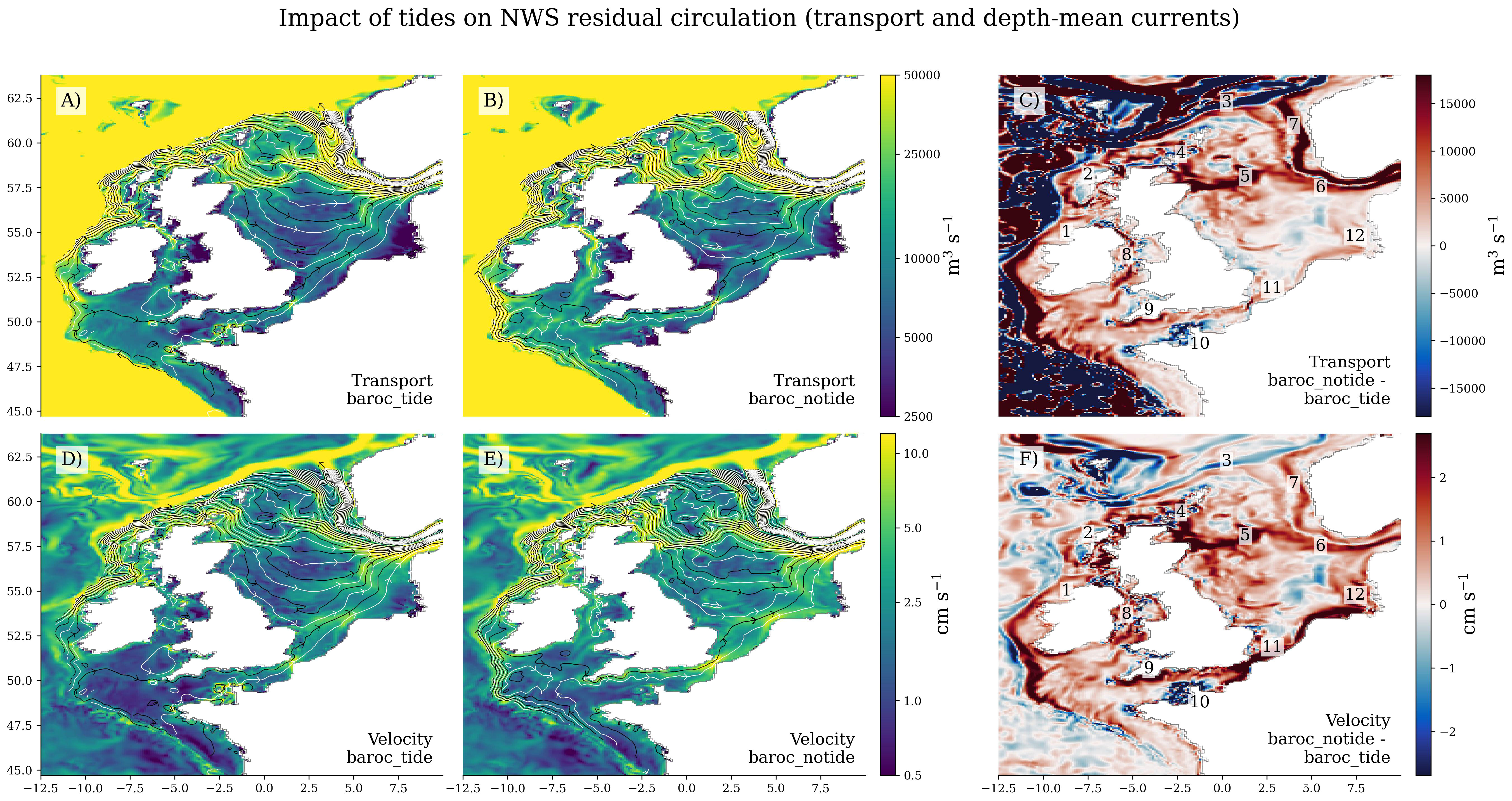
Figure 1 NWS Winter residual circulation in terms of volume transport (m³ s^-1, A–C) and depth-mean velocities (m s^-1 D–F) for baroc_tide (A, D) and baroc_notide (B, E), and their differences (C, F). baroc_tide and baroc_notide are the simulations with and without tides and are defined in section 2.2. The colouring shows the magnitude (on a logarithmic scale) of the transport (A, B) and velocity (D, E), while the streamlines (and arrows) show the direction. The streamlines are alternately coloured black and white for clarity. (C, F) shows the difference in magnitude of transport (C, m s^-1) and velocity (F, cm s^-1) between baroc_notide – baroc_tide, showing regions where baroc_notide is greater than baroc_tide in red. The numbers in (C, F) refer to pertinent circulation features, which are described in Box 1.

BOX 1 Pertinent features of NWS circulation, as shown in Figure 1 (and Supplementary Material Figure 1). Box adapted from Tinker and Hermanson (2021).
NWS circulation features that are relevant to this study are numbered in the panels of Figure 1: The shelf slope current (1, 2, 3) follows the shelf break (~500m isobath). Inshore of this, 1) The Irish Coastal Current links to the Scottish Coastal Current, and then 4) the northern North Sea inflow; 5) and the Dooley Current (following the 100 m isobath) connects to the 6) inflow into the Skagerrak, which retroflects, and flows out as 7) the Norwegian Coastal Current. baroc_notide (and GloSea5) has an incorrect flow through the Irish Sea 8), which continues along the northern (English) coast of the English Channel (9) – in baroc_tide (and CMEMS and in reality) the stronger western English Channel currents are along the French Coast, and around the Channel Isles (10), associated with substantial tides. The southern (English Channel) North Sea Inflow follows a different pathway through the Southern Bight (11) and the German Bight (12) in baroc_notide (and GloSea5) and baroc_tide (and CMEMS), with the baroc_tide flowing mainly to the west of 11 and 12, and the baroc_tide flow to the east of 11 and 12.

GloSea5 had a cold fresh bias in the Irish Sea, English Channel, and southern North Sea (Supplementary Material Figures 2C, F) when compared with CMEMS. This is consistent with an (incorrect) southward residual current through the Irish Sea and into the English Channel bringing colder fresher water, as it mixes with the warmer, saltier water from the Celtic Sea and Atlantic. There is also a reduction in salinity predictability in this region, consistent with advected variability having an incorrect providence. GloSea5 has a salty bias around Scotland (e.g. ~58°N 2°W), consistent with currents in this region being too strong.

The English Channel is much warmer and saltier than in the southern North Sea in CMEMS, and so there is a visible warm salty plume into the Southern Bight (~52°N 3°E, from the Dover Strait). In GloSea5, the fresher cooler English Channel is (incorrectly) of similar temperature and salinity to the southern North Sea, so the plume is not visible.

Tinker and Hermanson (2021) used model data from GloSea5 to drive a regional shelf seas model (NEMO CO6) to dynamically downscale two winters as a case study – this improved the spatial resolution over the NWS, and added important shelf seas processes (including tides). The circulation errors (between GloSea5 and CMEMS) reduced in these downscaled simulations, as did the temperature and salinity biases. They speculated that the improved circulation was responsible for the reduced temperature and salinity biases, and while they suggested that the inclusion of tides in CO6 explained these circulation improvements, they did not explore this further.

1.2 Study outline

In this study we investigate the role that tides play in the residual circulation of the NWS, and the resulting temperature and salinity distribution. We focus on winter circulation because during this period the NWS is largely well mixed and so baroclinic processes are less important, and to help explain the results described in Tinker and Hermanson (2021). To this end, we focus on the following scientific questions:

Is the NWS winter residual circulation different with and without tides?

What is the impact of tides on:

a. the spatial pattern of the mean residual flow?

b. the variability of the mean residual flow?

c. the (volume) transport through cross-sections?

2. What are the implications for temperature and salinity distribution?

a. What are the possible mechanisms leading to the differences?

i. Can these be parameterised into non-tidal models?

We first describe the model and techniques we use in the methodology section. In the results section we compare the average winter depth-mean NWS residual circulation maps with and without tides. We consider differences in the distributions in the residual flow (with respect to inter-annual variability) with and without tides, and consider whether the differences are significant. We compare time-series of transport through cross-sections with and without tides, noting that residual transport, residual currents and advective pathways are related but different parameters. We assess the impact of tides on the spatial distribution of temperature and salinity. We then consider different mechanisms by which the tides may influence the residual current and investigate whether these may be parameterised into non-tidal models. Finally, we discuss the results and draw conclusions in the discussion and conclusion sections.

2 Methods

We ran sensitivity studies of the NWS to simulate the effect of tides on the residual flow structure. We used the NEMO Coastal Ocean Model version 6 (CO6) as our shelf seas model, and dynamically downscaled a GCM (HadGEM3) present-day control simulation as used by Tinker et al. (2020).

We now introduce the models, and the simulations with our experimental design. We also describe the analysis techniques we will use. We introduce several abbreviations, so include their definitions in Table 1.

TABLE 1

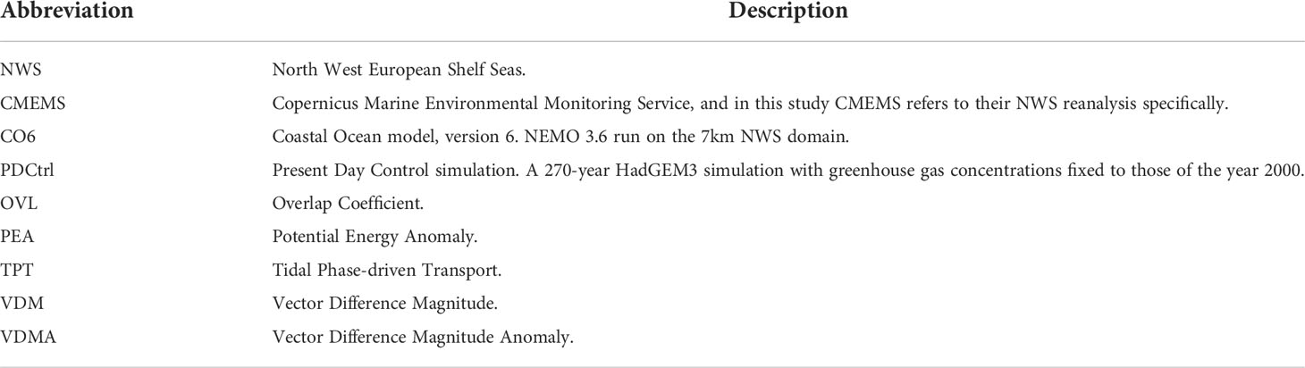
Table 1 Abbreviations introduced in this study.

2.1 Models

2.1.1 GCM present-day control simulation

We give a brief description of the present-day control simulation of HadGEM3 GC3.0 (hereinafter PDCtrl) and the simulations, and refer the reader to Tinker et al. (2020) for full details.

HadGEM3 GC3.0 (Williams et al., 2018) is a Met Office CMIP6 GCM. The ocean component is NEMO (Madec and NEMO Team, 2016) run in the ORCA025 configuration (Storkey et al., 2018) – ~¼° horizontal grid (~17 km on the NWS) with tidal dissipation being parameterised, rather than being modelled as dynamic tides.

For the PDCtrl, the greenhouse gas concentrations, ozone concentrations and aerosol emissions were kept constant (or with a repeating annual cycle) at year 2000 levels. This simulation represents the near present-day for the duration of the (270 year) model run (e.g. all model years between 1980 and 2250 represent conditions consistent with the year 2000). This simulation has been assessed (for the model years 2030-2080) by Williams et al. (2018), and Tinker et al. (2020) undertook additional assessment for the NWS region.

PDCtrl was run with a 360-day calendar. In order to create forcings for the Gregorian calendar (as used here), we repeated the forcings from the 30^th of January, March, May, July, August, October, and December (to give data for the 31^st of those months), and ignored the data from the 29^th and 30^th of February (for common years).

2.1.2 Downscaling tidal model: NEMO CO6

CO6 (O’Dea et al., 2017) is a primitive equation, Boussinesq, 3D baroclinic hydrodynamic model, with a non-linear free surface, and is run on a 7 km NWS domain. This domain extends from 40°4’N 19°W to 65°N 13°E, with a 1/9° by 1/15° resolution (longitude and latitude respectively, ~7km), and 50 hybrid terrain following vertical levels (Siddorn and Furner, 2013). CO6 is a well-established model, being used operationally at the Met Office, as the basis of the Copernicus NWS reanalysis (Renshaw et al., 2019), and as a research tool (Hermans et al., 2020; Tinker et al., 2020; Tinker and Hermanson, 2021).

CO6 simulates the tides directly, forced by the primary 15 tidal constituents of the NWS (M₂, S₂, N₂, K₂, K₁, NU₂, O₁, L₂, 2N₂, MU₂, T₂, M₄, Q₁, P₁, S₁) for both elevation and barotropic currents, taken from a tidal model of the North Atlantic (Flather, 1981). These are added to the ocean lateral boundary conditions and as tide generating forces in the model interior. The CO6 tides are assessed by (Renshaw et al., 2019) in the Copernicus reanalysis.

We briefly describe the downscaling technique – please refer to Tinker et al. (2020) for further details. We used model output from PDCtrl to provide our atmosphere and ocean boundary conditions for CO6 (hourly wind and pressure data, 6-hourly heat and freshwater fluxes, and daily-mean three-dimensional ocean temperature and salinity, barotropic velocities and sea surface height). We use a climatology for the river forcings, and for the exchange with the Baltic Sea.

2.2 Experimental design

We explore the impact of the tide on the winter NWS circulation by downscaling 10 years of PDCtrl with CO6, with and without tides. These simulations are referred to as baroc_tide and baroc_notide, respectively. When simulating without the tides, we do not add the 15 tidal constituents to the ocean lateral boundary conditions, or as tidal generating force. Otherwise, the two simulations are identical. We discard the first 11 months of the simulation as spin up. As we are mainly interested in tides and barotropic processes the model spins up quickly, and we consider this to be sufficient spin up time. The results are not qualitatively different when we increase the spin up time by another year, or in equivalent simulations with 10-year spin-up periods.

We develop two proof-of-concept parameterisations to simulate the effect of the tide on the residual circulation in non-tidal models. These are individually assessed in a pair of simulations (referred to as baroc_notide_TPT and baroc_notide_modCD), and in combination (referred to as baroc_notide_TPT_modCD). These parameterisations and simulations are described in Simulating the impact of tidal processes in non-tidal models.

During the winter the NWS is vertically mixed in most places, however in the non-tidal simulations the reduced mixing may allow stratification. We show that without tides, while there is localised stratification, the winter NWS is still largely mixed in baroc_notide. We focus on the winter, but briefly discuss the results in a summer context in the discussion.

2.3 Definition of the tidal residual currents

We have defined the tidal residual current as being the non-tidal part of the current. This can be calculated by removing the oscillating tidal signal from the modelled current velocities. The tides can be removed with a tidal filter such as the Doodson filter (e.g. Pugh, 1987), by a harmonic analysis, or simply by taking 25 hour or even monthly means. We typically used a Doodson filter described below.

2.4 Doodson tidal filtering

We de-tided the hourly currents with a Doodson tidal filter (e.g. Pugh, 1987) before averaging up to monthly means. However, we found that using monthly means, without filtering, gave very similar results. We compared the monthly means made of hourly data, with those made up of (Doodson) de-tided hourly data in Supplementary Figure 3. Using 11 years of monthly data (1980-1990, 132 months) of sea surface height and the depth-mean current components, we show that the two methods are highly correlated, that they have very similar variability and small biases.

2.5 Stream function from volume transport, and volume transport cross section

Volume transport is calculated online by CO6 (at every time step), and output as a daily mean product. The total horizontal transport (summed over all the vertical levels) is used to calculate the stream function: the model output volume transport is vertically summed, and then the northward volume transport component is cumulatively added from the east. The NWS model domain has a land boundary across the entire eastern boundary, and so knowledge of the stream function values at the open ocean boundary are not necessary.

Volume transport cross sections time series are calculated online by CO6 along predefined cross-sections (shown in Figure 3), and output as hourly means.

2.6 Residual current significance

Residual currents are vector quantities so many simple analysis techniques are not applicable. The eastward and northward components of the residual currents are typically normally distributed (Appendix Figure 1), but taken together have a bivariate normal distribution. This means their distribution is a Gaussian surface, rather than the Gaussian curve typical of scalar quantities (such as temperature). The maximum of this surface is centred on the mean current, and it decreases in all directions following a Gaussian curve. It has elliptical contours (contours of equal probability density) which vary from a straight line to an ellipse to a circle, depending on the variance and co-variance of the eastward and northward components. The volume under the surface integrates to 1. When plotting the residual currents (the northward component against the eastward component), most points (95%) fall around the mean current, within an ellipse that which encloses 2.45 standard deviation from the mean. By fitting uncertainty ellipses around the mean residual current (for a give number of standard deviations) we can simplify the description and analysis of the residual currents, allowing us to consider how steady a current is, and whether it is significant, given the inter-annual variability. Appendix section Probability Levels shows how the 2.45 standard deviations threshold is calculated from a chi-square distribution to capture 95% of the data.

When considering a normal distribution of a scalar property (such as temperature biases, or one of the velocity components), the mean ± 1.96 standard deviations encompass 95% of the data. When the absolute mean of a distribution is greater than 1.96 standard deviations, 0 is not within mean ±1.96 standard deviations, and the distribution is effectively significantly different from zero (at the 5% level). When considering a bivariate normal distribution, a 2.45 standard deviation ellipse centred on the mean residual current accounts for 95% of the residual current. If the origin is outside the 1 standard deviation ellipse, we consider the current to be “quasi-steady”. If the origin is outside the 2.45 standard deviation ellipse, we consider the current to be significantly different from zero.

We can use this approach to assess the similarity of two residual current distributions. In the Appendix (Supplementary Material Data Sheet 2) we give two methods for doing this, the more intuitive ellipse overlap method, and the more robust Overlap Coefficient (OVL, Inman and Bradley, 1989) method, which we use in this paper. When comparing two scalar distributions, the more their Gaussian distribution overlap, the more similar they are (Appendix Figure 2I). The OVL is the area under both Gaussian curves, and ranges from ~0 (distributions very different) to 1 (distributions are identical). We extend this method to compare 2-dimensional Gaussian distribution surfaces by integrating the volume under both surfaces. Full details of how this is calculated is given in the Appendix (Supplementary Material Data Sheet 2).

As our runs were 10 years long, we used the 30 individual winter months (December, January and February), rather than winter mean residual currents. This increases the variance (the size of the ellipses) and decreases the area of the NWS with significant currents.

A python library to calculate and analyse residual current uncertainty ellipses is available (Tinker and Polton, 2022, https://doi.org/10.5281/zenodo.6482468). See Appendix section Python Library for further details.

2.7 Vector difference magnitude and vector difference magnitude anomaly

To show the impact of different tidal parameterisations on the residual currents, we use the Vector Difference Magnitude (VDM) between the baroc_tide and a non-tidal run. We always use VDM to refer to differences from the baroc_tide simulation, and so it is only subscribed with the non-tidal run (referred to as _simulation in the following equation). VDM _simulation is defined as:

$\begin{array}{ll}VD{M}_{simulation}=\left| U_{baroc\_tide}-U_{simulation}\right| = \sqrt{{\left(u_{baroc\_tide}-u_{simulation}\right)}^2-{\left(v_{baroc\_tide}-v_{simulation}\right)}^2}& (1)\end{array}$

where U = (u, v) is the depth-mean residual currents at a given point and the subscript denotes the experiment name (baroc_tide, or _simulation being baroc_notide or one of the other non-tidal simulations). VDM represents the magnitude of the vector difference (in cm s^-1) between the two vectors, as illustrated in Supplementary Material Figure 10. Thus, VDM captures how different the two currents are in terms of magnitude and direction (e.g. Supplementary Material Figures 11 A–D).

We then ask if a different tidal parameterisation increases or decreases VDM (relative to the VDM_{baroc_notide}) using the Vector Difference Magnitude Anomaly (VDMA). For example, to ask if a tidal parameterisation (e.g. TPT) improves the circulation of a non-tidal simulation, we calculate the difference between VDM_{baroc_notide} and VDM_{baroc_notide_TPT}.

VDMA_{baroc_notide_TPT} is:

$\begin{array}{ll}\begin{array}{c}VDM{A}_{baroc\_notide\_TPT}=VD{M}_{baroc\_notide}-VD{M}_{baroc\_notide\_TPT}\\ =\left|U_{baroc\_tide}-U_{baroc\_notide}\right|-\left|U_{baroc\_tide}-U_{baroc\_notide\_TPT}\right|\\ = \sqrt{{\left(u_{baroc\_tide}-u_{baroc\_notide}\right)}^2-{\left(v_{baroc\_tide}-v_{baroc\_notide}\right)}^2}\\ -\sqrt{{\left(u_{baroc\_tide}-u_{baroc\_notide\_TPT}\right)}^2-{\left(v_{baroc\_tide}-v_{baroc\_notide\_TPT}\right)}^2}\end{array}& (2)\end{array}$

VDMA always refers to difference from VDM_{baroc_notide}, and so is only subscripted with the name of the tidal parameterisation simulation. VDMA is also illustrated in Supplementary Materials Figure 10B. When VDMA is negative, the tidal parameterisation results in depth-mean residual currents that are closer to baroc_tide (at that point), and when it is positive, the tidal parameterisation increases the difference from the baroc_tide.

3 Results

We simulate the NWS winter circulation, with and without tides, to assess the impact of tides on the residual circulation, and on temperature and salinity distributions. As explained below, these simulations show similarities and differences to the data assimilating CMEMS reanalysis and the GloSea5 GCM simulations described by Tinker and Hermanson (2021) (Supplementary Material Figure 1). We show that the tides affect the circulation, and temperature and salinity distributions of the NWS, particularly through the Irish Sea, English Channel, Dover Strait, and the southern North Sea.

3.1 Evaluation

Our model sensitivity studies are very similar to Tinker et al. (2018) and have been evaluated in their study. We have undertaken additional evaluation to show that our model runs simulate the tidal processes sufficiently for this work (included in the additional Supplementary Materials). Supplementary Material Figure 4 shows the co-tidal charts for the dominant 4 tidal constituents, as well as the M₄ shallow water component, and the root mean squared difference error term (between baroc_tide and the harmonic analysis) which quantifies residuals not captured by the 15 tidal constituents of the tidal analysis.

Interactions between the M₂ constituent and higher, shallow water harmonics, can lead to tidal asymmetry with unequal peak flood and ebb flows (as shown by Piano et al., 2017). This shouldn’t have an implication to the net transport (the sum of multiple cosine waves integrates to zero), however, bed stress and energy flux are functions of the second and third power of velocity, and these do not necessarily integrate to zero over a tidal cycle (Domingues et al., 2008). Supplementary Material Figure 5A shows the bed stress resulting from the M₂-M₄ asymmetry (a mechanism that drives sediment transport). Our model simulates the realistic pattern as shown by Pingree and Griffiths (1979). The phase difference between the M₂ surface elevation and M₂ depth-averaged current shows where the M₂ tide is classified as a progressive wave (peak tidal currents occurring towards High and Low Water) or a standing wave (peak tidal currents occurring mid-way between High and Low Water) - our model simulates the realistic pattern as shown by Ward et al. (2018).

3.2 The impact of tides on circulation

We consider the pattern of the residual circulation, the variability around this, and we also consider volume transport through selected cross-sections, as these can provide quantitative evidence on temporal changes, at the expense of spatial resolution.

3.2.1 Differences in the residual circulation

There is a general agreement in the climatological winter mean NWS residual circulation between the simulation with tides (baroc_tide) and the simulation without tides (baroc_notide) (Figure 1), but there are some important differences. The removal of tides increased the transport: 82% of the seaspace of the NWS had depth-mean current magnitudes which were greater in baroc_notide than baroc_tide – this equated to an average increase in residual velocity magnitude over the NWS of 39% (0.77 cm s^-1) (comparing Figures 1E, D, red areas in Figures 1C, F). This is particularly clear inside the shelf break, where the slope current appears to (unrealistically) extend further onto the shelf in baroc_notide. The North Sea inflow ([4]), the Dooley Current ([5]) and the flow in and out of the Norwegian Trench ([6 & 7]) are all greater in baroc_notide than in baroc_tide. Additionally, baroc_notide simulated greater transport in many coastal regions, such as along the southern coast of southwest England, and along the European coast adjacent to and east of the Dover Strait. This suggests a tidal mechanism which reduces the residual velocity over large areas of the NWS. Conversely, weaker transport was simulated with baroc_notide in the southern English Channel and in parts of the Irish Sea – both regions of important tidal processes where tidal currents regularly exceed 1 m s^-1 (Robins et al., 2015), and in the southern central North Sea. This suggests a different tidal mechanism that increases the residual currents in locations with large tidal currents.

The northward Shelf Break Current follows the 500m isobar around the western (and north-western) edge of the NWS. It is driven by the Joint Effect of Relief and Baroclinicity (JEBAR, Huthnance, 1984), and acts to quasi-isolate the NWS from the North Atlantic (Wakelin et al., 2009). It is well reproduced in baroc_tide, but it flows onto the shelf in the Celtic Sea in baroc_notide, and tends to extend further onto the shelf right around the NWS shelf break. This leads to much greater residual current magnitudes around the western edge of the NWS in baroc_notide (than baroc_tide; e.g. [1], [2], [3] in Figures 1C, F).

In the Celtic Sea, there is a fairly persistent westward flow, with water in the southern Celtic Sea tending to flow into the English Channel, and water in the north tending to flow into the Irish Sea. This is captured by baroc_tide, whereas in baroc_notide the Celtic Sea currents are variable (in terms of inter-annual variability, Figure 2B).

FIGURE 2

Figure 2 Variability of the residual circulation climatology. (A, B) The significance of the residual current at the 5% level (shown in bold). When the 1 standard deviation ellipse does not include zero, the (quasi-steady) current is shown shaded. See text and appendix for further details. (C) The ratio of the mean current variability (the area of the baroc_tide 2.45 standard deviation ellipse divided by that of baroc_notide). Over most of the shelf, there is much greater variability in baroc_notide. (D) The similarity of the residual current distributions of the two simulations as quantified by the Overlap Coefficient (OVL, see Residual current significance and the Appendix for details): the integrated volume under the two Gaussian distribution surfaces. Where the distributions are very different, OVL≈0, where the distributions are identical OVL=1. Contours in (C, D) increment every 25% (0.25).

In the Irish Sea there is a significant northward current along the eastern coast of the Irish Sea (i.e. from western Cornwall (50.75°N 5°W) to south Wales (51.5°N 5°W), and from northwest Wales (53.25°N 5°W) towards the North Channel (55°N 5.5°W) which is captured by baroc_tide whereas in baroc_notide, there is a southwards current flowing through the North Channel, down the centre of the Irish Sea, and into the Celtic Sea (Figure 1B). Despite these fundamental differences, both simulations have a net northward transport though the Irish Sea (Figure 3).

FIGURE 3

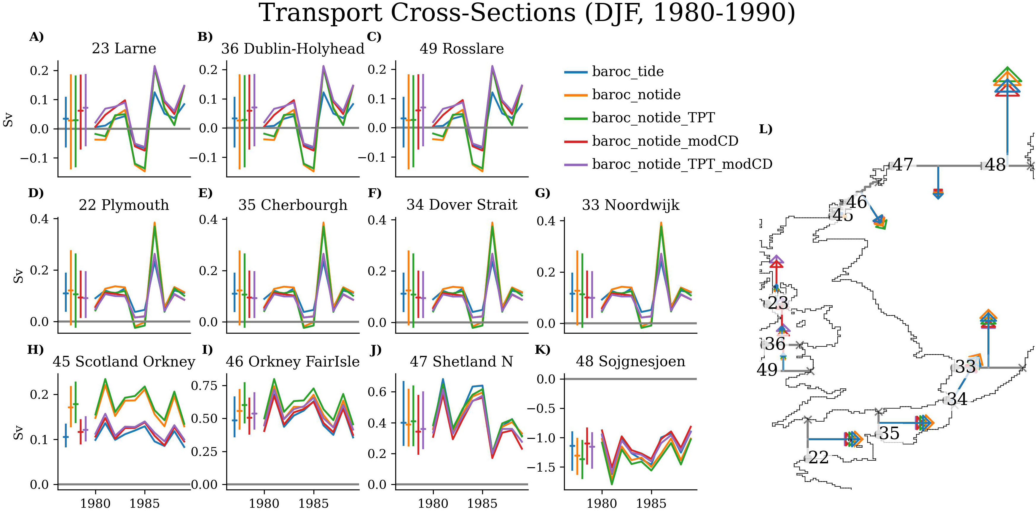
Figure 3 NWS Winter (DJF) volume transport time-series through selected cross-sections (A–K). (L) map showing volume cross-section locations, with coloured arrows showing the direction and relative magnitude of transport for each of the model simulations. Left hand panels (A–K) volume transport time series through cross-sections in (L). To the left of each time series is a series of crosses, denoting the time series mean, and 5^th and 95^th percentiles. (A–C) Irish Sea cross-sections, (D–G) English Channel cross-sections, (H–K) northern North Sea inflow/outflow cross-sections.

There is a net eastward transport through the English Channel. The tides are stronger along the French coast, and these large tides drive non-linear elevation-current interactions, which lead to stronger residual circulation along the French coast of the English Channel than the English coast. The above residual circulation pattern was well captured with the baroc_tide simulation. Conversely, in the baroc_notide, the flow is (unrealistically) concentrated along the English coast.

Both the English Channel, and eastern Irish Sea are regions of large tides. A tidal mechanism that acts to increases the residual current speed would help explain the difference between baroc_tide and baroc_notide in these regions.

3.2.2 Residual flow variability and significance

There are also differences in the inter-annual variability (over the 10-year simulations) about the mean residual currents in the baroc_tide and baroc_notide NWS simulations (Figures 2A, B). For a given location, the residual currents from each simulation form a distribution, which is summarised as an uncertainty ellipse. By considering the properties of these ellipses, we can simplify the description and analysis of the currents. First, we look at the significance of the mean residual circulation by seeing if the origin is within the uncertainty ellipse (i.e. whether the mean residual current is greater than 2.45 standard deviations of its variability - see Residual current significance and the Appendix for details) for the two simulations, and show where they differ. We then compare the magnitude of the interannual variability of the residual circulation. Finally, we consider the similarity of the distributions of the residual currents in the two simulations (in terms of residual current Overlap Coefficient, OVL).

In most regions, the residual currents vary inter-annually in their location and magnitude – as such these currents are rarely significant, although can often be considered quasi-steady (with their mean greater than 1 standard deviation rather than 2.45). Where residual currents are persistent over time (e.g. topographically constrained), they are often significant.

In particular, the main circulation structure that feeds into the North Sea northern inflow ([4]), and the transport either side of the Norwegian Trench ([7]) are significant in both baroc_tide and baroc_notide (Figures 2A, B), with similar spatial extents, although they appear to have a greater magnitude in baroc_notide.

Away from the main northern North Sea inflow, there are several regions where there is a significant residual current that is present in the baroc_tide but absent in baroc_notide. The East Anglia Plume (~53°N 3°E, the eastward extension of the southward current along eastern Britain) is significant in baroc_tide but is not significant in baroc_notide. The northward currents along the north Devon coast and the south coast of Wales (shown in Figure 1A) are significant in baroc_tide, as are the currents northward from northwest Wales – these are all absent or not significant in baroc_notide. The waters around Channel Islands and Cotentin Peninsula (~49.75°N 2°W, Normandy) have very large tides, and in this region baroc_tide has strong significant eastward residual currents that are absent in baroc_notide. The strong eastward current along the southwest British coast of the English Channel in baroc_notide is not significant. Currents that are stronger but less significant in baroc_notide (than in baroc_tide) are likely to be more variable in baroc_notide. If a tidal process predominantly drives a residual current in one direction, its likely to reduce the variability, and increase the significance, even if the mean velocities are lower.

We can compare the magnitude of the variability of the residual flow (Figure 2C). The ratio of the areas of the residual current ellipses shows that the inter-annual variability of the mean residual flow of baroc_tide is substantially less than that of baroc_notide over most of the NWS (Figure 2C). In the Irish Sea, English Channel, and southern North Sea, the baroc_tide (2.45 standard deviation) ellipses are less than 25% of those of baroc_notide. Central and northern North Sea, and the Irish and Shetland shelves are closer to 50-75%. However, in the southwest Celtic Sea, the shelf break, Norwegian Trench and isolated regions across the NWS, the baroc_tide had a greater variability in the mean residual current. Most regions with large M₂ tidal amplitudes (Supplementary Material Figure 4) have lower residual currents variability in baroc_tide than in baroc_notide, again suggesting that tides reduce the variability of the residual circulation.

Finally, we compare the similarity of the residual current distributions of the two simulations (Figure 2D). We use the OVL (Overlap Coefficient, described in Residual current significance and in the Appendix) to quantify the similarity integrated over the whole distribution. For given point, when the distributions are identical (same mean, variance and covariance), the OVL is 1, and this deceases towards 0 as the distributions diverge. OVL captures both the change in the mean and the variability of the residual currents.

OVL (Figure 2D) effectively shows where the tides affect the distribution of residual currents. The OVL is relatively high to the north of Ireland, the eastern North Sea and Norwegian Trench reflecting a similarity of the residual current distributions in both baroc_tide and baroc_notide, suggesting that the residual current are relatively insensitive to the tides in these regions. Conversely, in the English Channel, Irish Sea, and Southern Bight ([11]), and around the east coast of Scotland, the OVL is low, suggesting a difference between the two models, and that tidal processes play an important role in the residual currents in these regions. OVL is similar to the inverse of the M₂ amplitude (Supplementary Material Figure 4), with higher tides in the eastern Irish Sea, Celtic Sea, English Channel and western (and southern) North Sea being co-located with lower OVL values.

3.2.3 Quantitative volume transport cross-sections

Volume transport cross-sections through the Irish Sea, English Channel and North Sea northern Inflow are described in Figure 3 and Table 2. Transport cross-sections are an important component of budget analysis, but cannot be directly interpreted for connectivity issues, such as the advective pathways and water body providence. For example, if we are interested in the origin of the English Channel water, and a particular model simulation has a continuous current flowing through the North Channel, down the Irish Sea, and into the English Channel, with a very clear providence and connectivity, this could be very clear in the transport cross-sections. Or, there could be an unrelated counter current flowing north, which masks this connectivity in the transport cross section.

TABLE 2

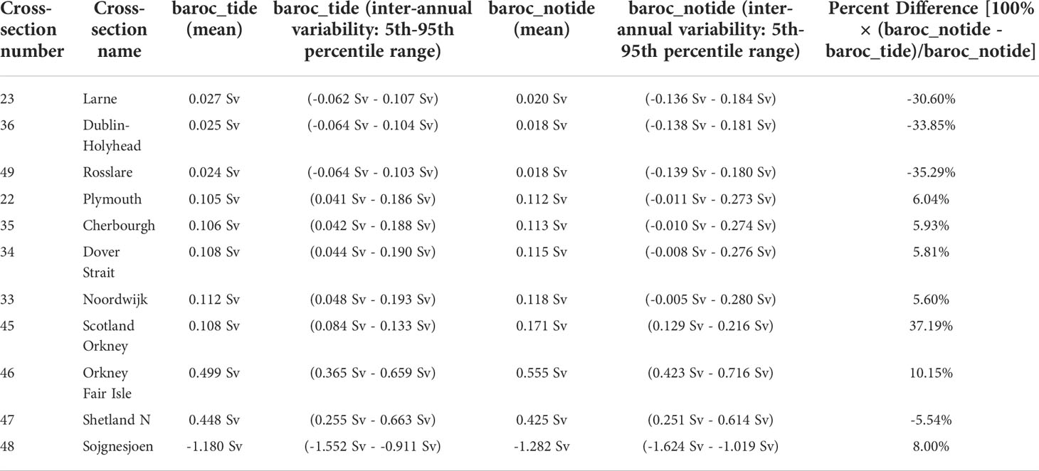
Table 2 Mean transport through cross-sections for baroc_tide and baroc_notide.

The northward flow through the Irish Sea was substantially weaker (~30%) in baroc_notide than in baroc_tide. Furthermore, the transport inter-annual variability was substantially greater in baroc_notide; However, the difference is not significant, and there were some years when the baroc_notide is stronger than baroc_tide.

The flow through the Dover Strait ([11]) and into the southern North Sea was ~6% stronger in baroc_notide than baroc_tide (through model cross sections 35, 34 and 33). Again, there was more transport inter-annual variability in the baroc_notide than in baroc_tide.

The northern North Sea inflow (between Scotland and Shetland, [4]) was greater in baroc_notide than baroc_tide, particularly via the Fair Isle Current (Figure 3, section 45, 37% stronger). There was little difference in the inflow to the east of the Shetlands (section 48), but the Norwegian Trench outflow is 8% stronger in baroc_notide than in baroc_tide.

There was considerable inter-annual variability in the net transport, and so there was seldom any significant difference between the baroc_tide and baroc_notide (section 45 being an exception). Analysis of the time series of the positive and negative components of the transport may illuminate more subtle differences, but the tidal oscillations make this difficult and less meaningful. It was interesting to note that in the Irish Sea and English Channel profiles (Figures 3D–G) inter-annual variability was typically stronger in the baroc_notide than in baroc_tide.

3.2.4 The impact of tides on temperature and salinity

Tinker and Hermanson (2021) suggested that some of the differences in temperature and salinity between GloSea5 and CMEMS, and their predictability, can be explained by the difference in the circulation. Here we assess the impact tides have on the temperature and salinity distributions.

The winter NWS SSTs are generally cooler without tides (Figure 4), although in most regions this is insignificant. There are large regions of the Irish Sea, northeast Celtic Sea and English Channel that are significantly cooler (up to 0.8°C) without tides. The same regions are significantly fresher without tides, although the fresher region extends through the Dover Strait and the Southern Bight, across the German Bight (without entering it – there is a small region with a significant increase in salinity in the coastal interior of the German Bight), and approaches the Jutland Peninsula (~57°N 8°E) and the Kattegat/Skagerrak. The salinity distributions suggest that the transport of saline oceanic water across the Celtic Sea into the English Channel and Irish Sea is weaker without tides.

FIGURE 4

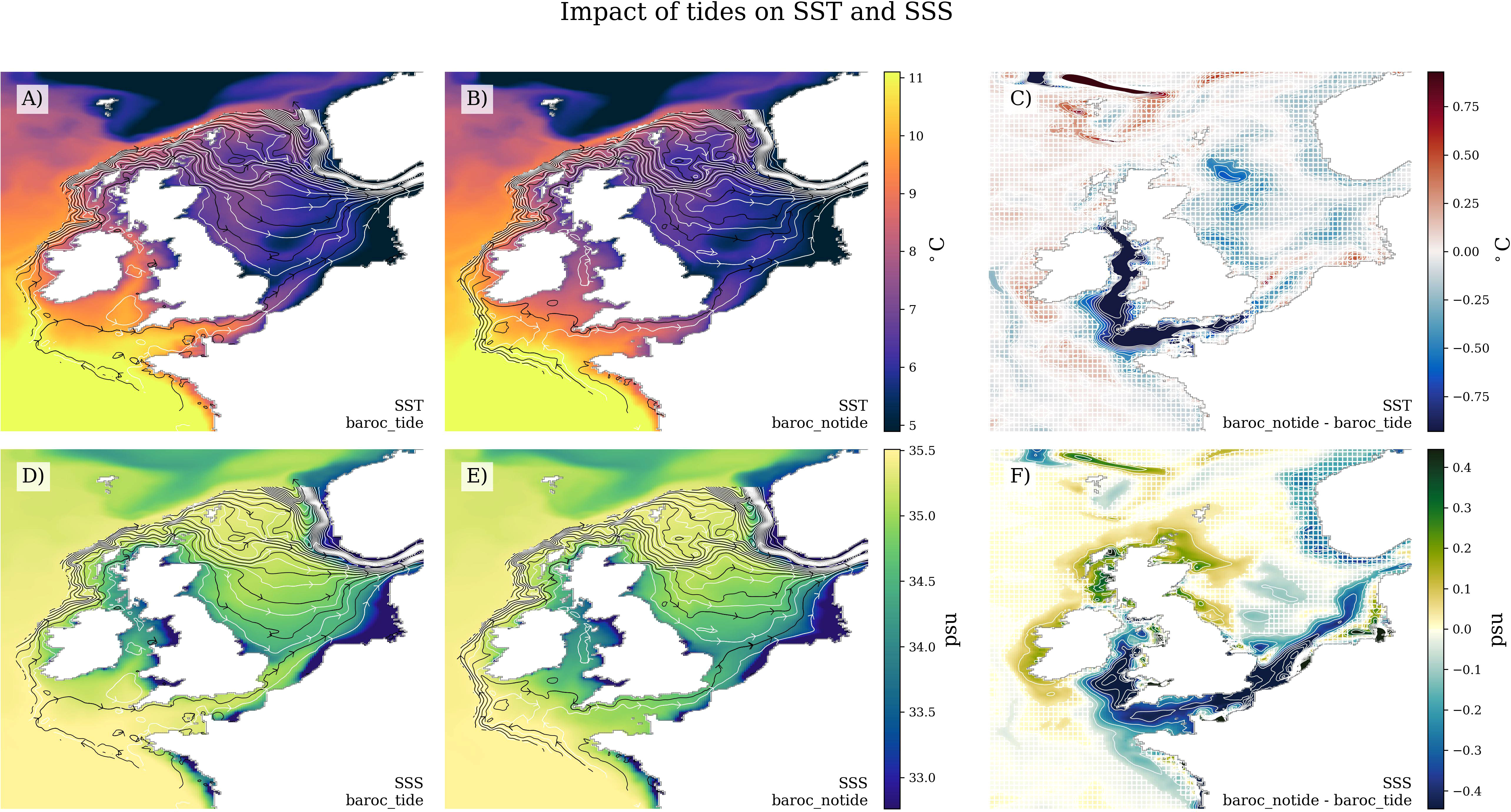
Figure 4 The impact of tides on the NWS winter mean SST and SSS. (A, B), baroc_tide and baroc_notide mean SST with stream lines (from Figure 1). (C) Absolute difference between baroc_notide and baroc_tide with white hatching showing where the difference is not significantly different with a T-Test at the 5% level. (D–F), equivalent to (A–C) but for SSS.

There is a significant increase in salinity (without tides) to the west of Ireland and west and north of Scotland, and through the northern North Sea inflow. This is consistent with the greater Scotland-Shetland North Sea inflow transporting saline Atlantic water into these regions. Many coastal regions have significant increase in salinity (without tides), including parts of the west and east coast of the UK, and the European coast north and west of Rhine and the Elbe – tides play an important role in such Regions of Freshwater Influence (ROFIs; e.g. Simpson, 1997).

The difference between SST (and SSS) caused by tides (i.e. the difference between baroc_tide and baroc_notide) is remarkably similar to the difference between the CMEMS reanalysis (with tides) and GloSea5 simulations (without tides) (see Supplementary Material Figure 2F), in terms of both spatial pattern and magnitude. This suggests the GloSea5 temperature and salinity biases are associated with the missing tides.

In baroc_notide, there is a slight increase in stratification compared with baroc_tide (Supplementary Material Figure 6), although most of the NWS is still considered fully mixed (Potential Energy Anomaly (PEA) < 10 J m^-3). Baroc_notide has an unrealistic ribbon of salinity driven stratification up the centre of the Irish Sea (PEA ~50 J m^-3), temperature and salinity driven salinity in the northern Celtic Sea, and a small region of temperature driven stratification in the western approaches of the English Channel (Supplementary Material Figures 7, 8). The baroc_notide-baroc_tide SST and SSS anomalies do not simply reflect this change in stratification, as they are present in the Near Bottom Temperature and Salinity (NBT and NBS respectively) (to greater/lesser extent that in SST/SSS, see Supplementary Material Figure 8).

3.3 Theoretical mechanisms linking tides and residual circulation

We have shown important differences in the mean flow and tracer fields (temperature and salinity) between the simulations with and without tides. We have speculated about a possible tidal mechanism which tends to reduce the mean velocity over most of the NWS, and another which increases the mean residual current, and perhaps reduces its variability. There are a several tidal mechanism which interact with the residual circulation (e.g. see Robinson (1983) for overview). We now investigate two of these tidal mechanisms that affect the residual flow field, and may fill these roles. As well as considering local effects, we note the connected nature of circulation allows remote mechanisms to have a local effect.

Firstly, the phase difference between the timings of high water and slack water can drive residual circulation. Secondly, the greater instantaneous velocities associated with tides affect the bed stress and friction that can impact residual circulation. Here we consider these in turn.

3.3.1 Tidal phase difference driven transport

Transport is the product of (depth-mean) velocity and the depth of water, therefore differences in the phase of the surface elevation and velocity tidal cycle can lead to a residual transport. This concept is seen elsewhere in the oceanographic literature as a “bolus” transport (Rhines, 1982; McDougall, 1991; Marshall, 1997). In shallow water it is manifest, for example, if the peak flood occurs during high water (i.e. a progressive wave) and transports more water than the peak ebb at low water (Prandle, 1997). We refer to this mechanism as Tidal Phase-driven Transport (TPT). It is similar to Stokes Drift in wind-wave transport, although strictly speaking Stokes Drift is driven by the wave orbital motions, and as we are considering depth-mean flow, this is different. This term is the difference between the Lagrangian and Eulerian transport (Robinson, 1983).

We take a numerical approach, by calculating TPT as the northward and eastward components of the volume flux (Q_TPTu, Q_TPTv) over a complete M₂ tidal cycle (with 1000 time-steps):

$\begin{array}{ll}{Q}_{TPTu}={\displaystyle {\int }_{t=0}^{t=T_{M2}}}\frac{\left(a_{\eta }sin \left({\sigma }_{\eta }t+{\varphi }_{\eta }\right) +D\right)\left(a_{\widehat{U}}sin \left({\sigma }_{\widehat{U}}t+{\varphi }_{\widehat{U}}\right) \right)e_2^t}{T_{M2}}dt=\underset{\_}{\tilde{u}\tilde{h}}& (3)\end{array}$

$\begin{array}{ll}{Q}_{TPTv}={\displaystyle {\int }_{t=0}^{t=T_{M2}}}\frac{\left(a_{\eta }sin \left({\sigma }_{\eta }t+{\varphi }_{\eta }\right) +D\right)\left(a_{\widehat{V}}sin \left({\sigma }_{\widehat{V}}t+{\varphi }_{\widehat{V}}\right) \right)e_1^t}{T_{M2}}dt=\underset{\_}{\tilde{v}\tilde{h}}& (4)\end{array}$

where T, a, σ and ϕ denote the M₂ period, amplitude, frequency, and phase for sea surface height (η) and the depth-mean U and V velocity components. D gives the depth of water, and $e_2^t$ and $e_1^t$ give the northward and eastward grid box size (m). This can also be considered the time mean product of the tidally (sinusoidally) varying components of the velocity and depth ($\tilde{u}$, $\tilde{v}$, $\tilde{h}$).

We calculated the residual transport associated with this TPT for our simulations (Figure 5A). Many areas where the residual currents are increased with tides (Figure 1C) show substantial transport associated with the TPT. There is a clear northward transport through the Irish Sea, along the north Cornish and Devon coasts (~50.75°N 5°W), along the southern coast of the English Channel, all of which are missing in the GloSea5 simulation. It also enhances the cyclonic North Sea transport, the English Channel through flow, and the cross Celtic Sea flow. The TPT is reduced when the M₂ tide is a standing wave (e.g. Supplementary Figure 5B).

FIGURE 5

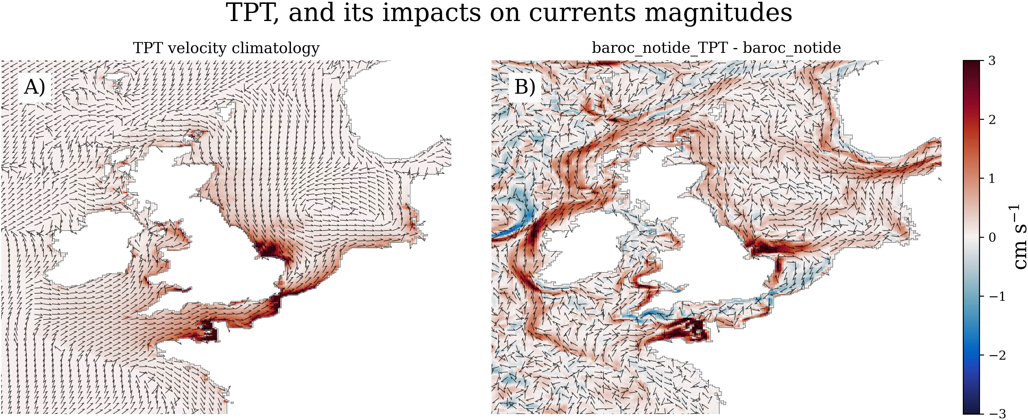
Figure 5 (A) Residual transport associated with TPT (cm s^-1), and (B) the impact the TPT tidal parameterisation has on the depth-mean current magnitudes (baroc_notide_TPT-baroc_notide). The colour denotes the change in magnitude (cm s^-1) and arrows give direction (not magnitude). Red shows where the current is faster in the tidal parameterisation simulation than in baroc_notide.

We also explored a related mechanism, that of tidal stress (Nihoul, 1980), which allows energy transfer between the mean and tidal flow. Like the TPT Mechanism, the tidal stress captures the Lagrangian advective term (u∇▪(u)) of the Navier-Stokes equation, however, as it is less applicable, we do not further investigate it. For further details, please refer to the supplementary materials.

3.3.2 Impact of tides on bed stress

We have seen that the tides tend to slow the residual circulation over most of the NWS. One possible mechanism is a change to the friction of the system.

To first order we are interested in understanding the balance of forces that modify the residual circulation. We are particularly interested in the role of tides on the residual circulation, which we can notionally separate into Eulerian (non-tidal) and Lagrangian (tidal) contributions:

$\begin{array}{ll}\frac{D\left(Tranport\right)}{Dt}=\raisebox{1ex}{$d$}\!\left/ \!\raisebox{-1ex}{$dt$}\right.\left(Eulerian Transport\right)+\raisebox{1ex}{$d$}\!\left/ \!\raisebox{-1ex}{$dt$}\right.\left(TPT drift\right)& (5)\end{array}$

In a steady state, the transport is then given by:

$\begin{array}{ll}f\times \frac{D\left(Tranport\right)}{Dt}=\left(pressure terms\right)+{\tau }_{top}-{\tau }_{bed}& (6)\end{array}$

Considering this balance, omitting tides will have a most significant effect through the τ_bed term. This is because bed stress is a non-linear term that varies with the mean magnitude of velocity (squared). In a non-tidal simulation (in the absence of a strongly oscillating flow), the bed stress is therefore underestimated because the instantaneous velocities are reduced. Other terms are not so directly affected by tides (though barotropic and baroclinic pressure gradients could be indirectly affected by mixing). We therefore conjecture that we could go some way to reconstruct the effect of tides in the transport equation by making the τ_bed term act as if it included tides. If τ_bed is an important term in closing the transport budget for a circulation with tides then the circulation will improve when τ_bed is parameterised to include tidal effects. If on the other hand τ_bed is not so important in the transport budget that determines the circulation under tidal forcing, then the circulation would not be expected to improve with a modified τ_bed. The drag coefficient in τ_bed is locally scaled to capture the missing drag from the oscillatory flow such that (τ_bed)_notide = (τ_bed)_tide.

Making the parameterisation a function of the flow, rather than just prescribing a drag, opens a route to developing a dynamic tidal parameterisation for coarse resolution shelf regions.

Friction with the bed leads to bed stress (τ_x and τ_y) as:

${\tau }_x=-C_{D}u\sqrt{u^2+v^2}$;

$\begin{array}{ll}{\tau }_y= -C_{D}v\sqrt{u^2+v^2}& (7)\end{array}$

Where C_D is the drag coefficient and u and v are the (instantaneous, hourly) bed velocities.

With a magnitude (||τ ||):

$\begin{array}{ll}\left|\right|\tau \left|\right|=\sqrt{{\tau }_x^2+{\tau }_y^2}= \left|C_D\right|\left(u^2+v^2\right)=\left|C_D\right|\left|\right|\mathbf{U}{\left|\right|}^2& (8)\end{array}$

The NWS bed stress magnitudes are substantially higher in baroc_tide compared with baroc_notide (Figure 6). This is particularly the case in the English Channel, Southern Bight ([11]) and Irish Sea, where the tides are strong. The bed stress directions do not agree with the mean residual circulation, or the difference between baroc_tide and baroc_notide mean residual circulation – highlighting the importance of other terms of the equation of motion.

FIGURE 6

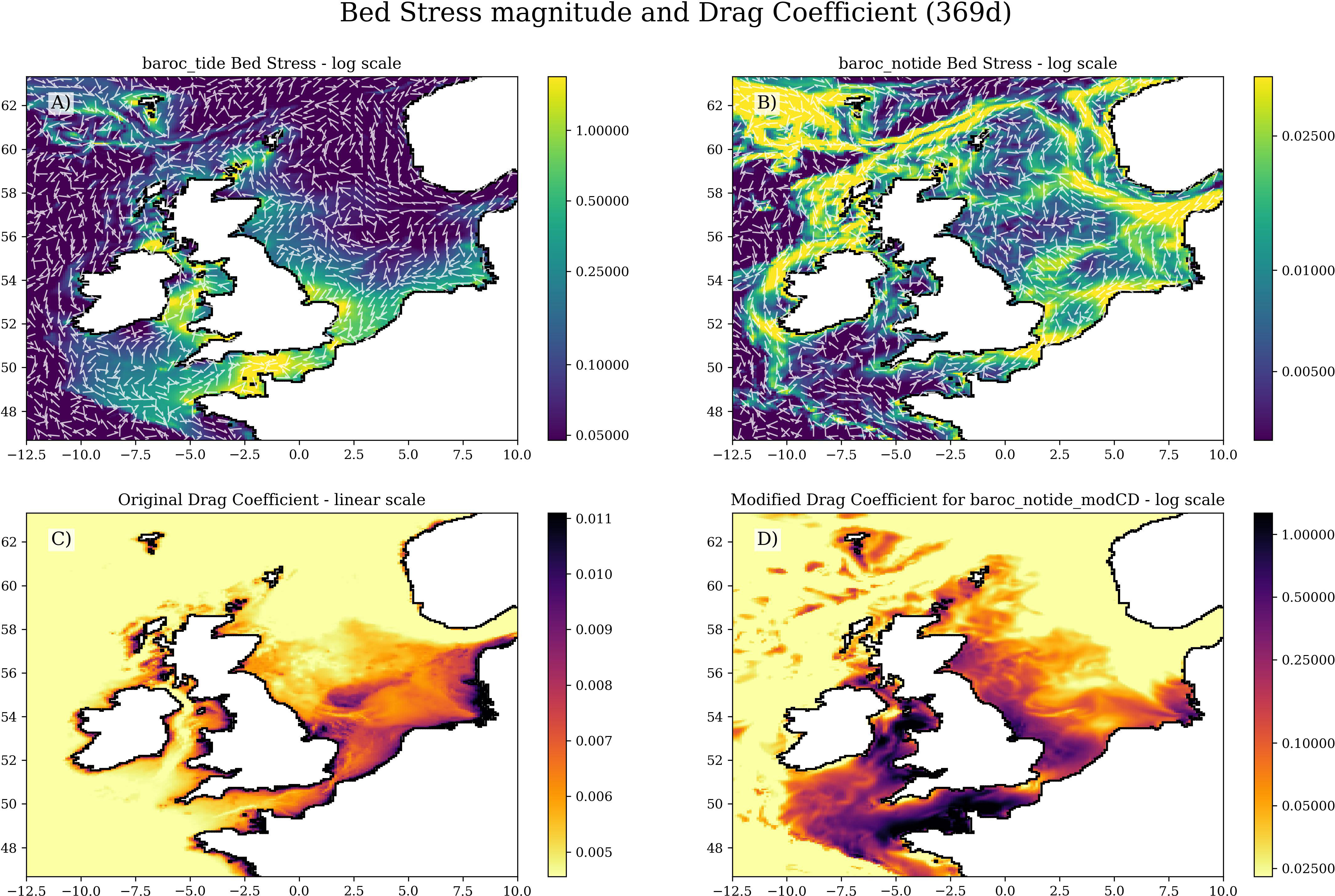
Figure 6 Bed stress magnitude (with arrows showing direction) and drag coefficients. (A, B) the mean bed stress in baroc_tide and baroc_notide respectively (both on log scale, but note the different ranges). (A, B) Are averaged over 369 days to average out the M₂ and S₂ constituents, and annual cycle. (C) The standard drag coefficient used in NEMO (used in both baroc_tide and baroc_notide), on a linear scale. (D) the modified drag coefficient (on a log scale, calculated from equation (10), used in baroc_notide_modCD) to increase the bed stresses in the non-tidal simulations to match that of the tidal simulations.

The differences in bed stresses in baroc_tide and baroc_notide may lead to differences in the mean SSH field, which would drive different residual circulations. Matching the momentum budget between baroc_tide and baroc_notide via the bed stresses may improve this aspect of the residual circulation. As both simulations have a common drag coefficient (Figure 6C), we can use the ratio of bed stress magnitudes (Figures 6A, B) to construct a drag coefficient for non-tidal simulations, C_DNoTide :

||τ||_Tide=||τ||_NoTide then

$\begin{array}{ll}\left|C_{\mathit{\text{DTide}}}\right|\left|\right|{\mathbf{U}}_{Tide}{\left|\right|}^2=\left|C_{\mathit{\text{DNoTide}}}\right|\left|\right|{\mathbf{U}}_{NoTide}{\left|\right|}^2& (9)\end{array}$

and therefore:

$\begin{array}{ll}\left|C_{\mathit{\text{DNoTide}}}\right|=C_D\frac{\left|\right|{\mathbf{U}}_{Tide}{\left|\right|}^2}{\left|\right|{\mathbf{U}}_{NoTide}{\left|\right|}^2}=\frac{\left|\right|\tau {\left|\right|}_{Tide}}{\left|\right|{\mathbf{U}}_{NoTide}{\left|\right|}^2}& (10)\end{array}$

This modified drag coefficient is presented in Figure 6D (note the logged scale and different limits compared with Figure 6C). We averaged this over 369 days (the modulus of 8856 hours and the M₂ period (12.4206 hr) is about 7 minutes, so the M₂, S₂ and annual cycle have been effectively removed) to give a modified bed drag coefficient.

3.4 Simulating the impact of tidal processes in non-tidal models

We have shown that the absence of tides affects the residual circulation, and also impacts the temperature and salinity fields. Most state-of-the-art global ocean (and climate) models do not simulate tides, and so their residual circulation and tracer distribution could be affected, as suggested by Tinker and Hermanson (2021). We have identified two mechanisms by which the tides can impact the residual circulation – the TPT, which acts to drive the mean current, and the modified bed drag, which acts to slow the mean current. We now attempt to parameterise these mechanisms, and incorporate them into NEMO CO6, to simulate the effect of tides in a non-tidal simulation.

We first describe the parameterisations, introduce an experimental design to test them, and then describe the effect they have on the residual circulation, and temperature and salinity.

To parameterise the effect of the TPT, we save the tidal mean fluxes from equation (3) and (4) (and illustrated as depth-mean velocities in Figure 5A). These are read in NEMO CO6 as an ancillary file. These fluxes are implemented as a force term by forming a vector cross product with the Coriolis term (f×u_TPT). This can then be added to the barotropic flux equation of motion every timestep:

$\begin{array}{ll}\frac{du}{dt}=+f\left(v+v_{TPT}\right)+\dots & (11)\end{array}$

$\begin{array}{ll}\frac{dv}{dt}=-f\left(u+u_{TPT}\right)+\dots & (12)\end{array}$

The baroc_notide simulation is repeated with this parameterisation, hereafter referred to as baroc_notide_TPT.

To parameterise the effect of the modified bed drag coefficient we have adapted NEMO CO6 to use the modified bed drag coefficient as calculated in equation (10) and shown in Figure 6D. We cap the drag coefficient to a maximum value of 2.2, the NWS 99.5^th percentile value of the modified drag coefficient. We have re-run baroc_notide with the modified bed drag coefficient (baroc_notide_modCD).

We also run a simulation with both the TPT and modified bed drag coefficient, here in after referred to as baroc_notide_TPT_modCD. These experiments are summarised in Table 3.

TABLE 3

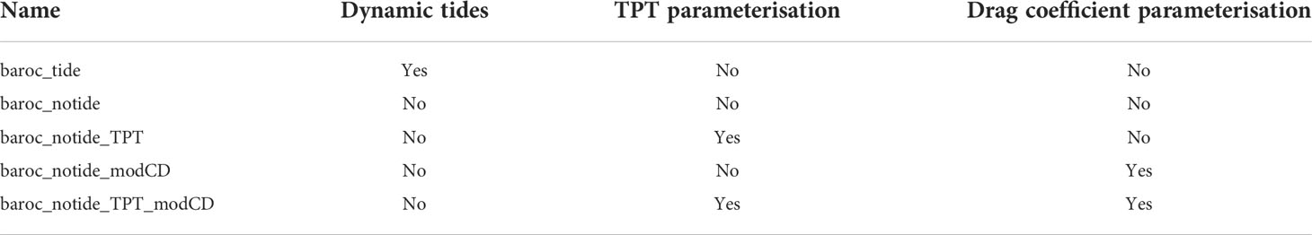
Table 3 Summaries of the experiments, including their treatment of the tide.

3.4.1 Assessing the impact of the tidal parameterisations

We first assess how these parameterisations affect the residual circulation, in terms of the mean and the variability, and then consider temperature and salinity.

The TPT parameterisation tends to increase the depth-mean residual velocity magnitude (as shown in Figure 5B as the difference in the magnitudes of the depth-mean residual velocities in baroc_notide_TPT minus baroc_notide). This is particularly clear along the coasts of north Cornwall and south Wales (51.5°N 5°W), the French coast of the western English Channel, and the English eastern coast – all regions where the TPT climatology is strongest. There is also an increase in the shelf break current, despite U_TPT being small in this region. The TPT parameterisation leads to a reduction in velocity magnitude along the south and southwestern coast of England (~50.25°N 4.5°W), weakening the unrealistic baroc_notide current here. There is also a slight reduction in the velocity magnitudes in the northern Irish Sea (away from the east coast).

Conversely, the modified drag coefficient tends to reduce the velocities across the shelf (Figures 7A, B), which is particularly clear along the path of the Dooley current ([5]), the western shelf break current (~51.5°N 11°W) and along the centre of the Irish Sea, and along the northern coast of the English Channel.

FIGURE 7

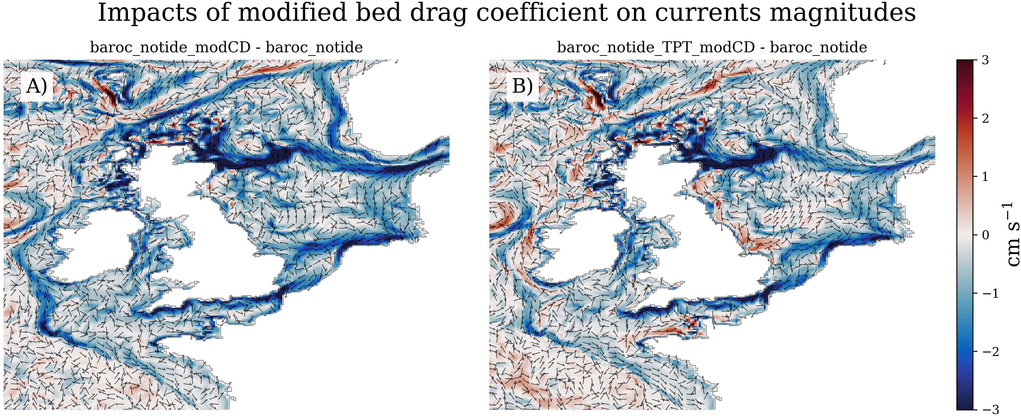
Figure 7 The impact the (A) modified bed drag coefficient tidal parameterisation has on the depth-mean current magnitudes (baroc_notide_modCD – baroc_notide) and (B) the impact of both the modified bed drag coefficient and TPT parameterisations (baroc_notide_TPT_modCD – baroc_notide). The colour denotes the change in residual current magnitude (cm s^-1) and arrows give direction. Red shows where the current is faster in the tidal parameterisation simulation than in baroc_notide.

When asking whether these changes in the mean velocities improve the residual circulation (becoming more similar to baroc_tide), we use the Vector Difference Magnitude Anomaly (VDMA, see Vector difference magnitude and vector difference magnitude anomaly for details). This quantifies how the Vector Difference Magnitude (cm s^-1, difference between the baroc_tide and a non-tidal simulation residual current vectors) changes with tidal parameterisation, showing where the parameterisation improves the residual circulation. Figure 8A shows the VDM for baroc_tide and baroc_notide, and Figures 8B–D shows how this changes with parameterisation (the VMDA for baroc_notide_TPT, baroc_notide_modCD and baroc_notide_TPT_modCD respectively), with negative values (coloured blue) showing where the tidal parameterisation has reduced the bias, and so improved the mean residual circulation.

FIGURE 8

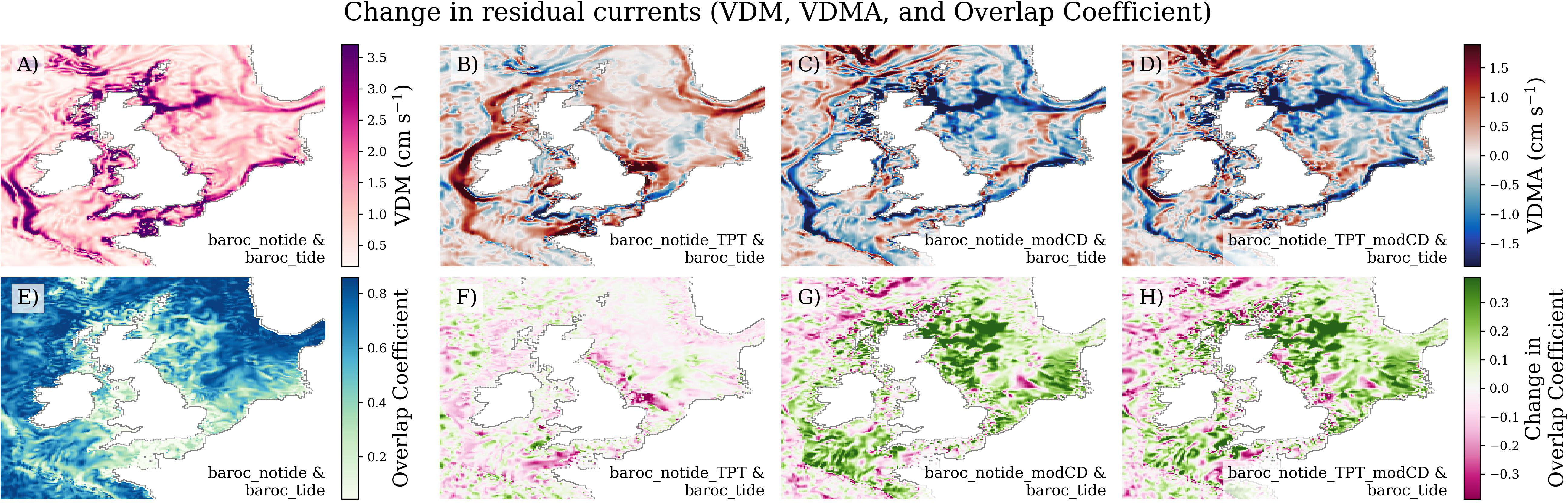
Figure 8 Impact of the tides and tidal parameterisations on the depth-mean residual flow, in terms of the mean (A–D) and the inter-annual variability (E–H). (A) VDM_{baroc_notide}, the Vector Difference Magnitude between baroc_tide and baroc_notide (lower numbers show greater agreement between the simulations), and (B–D) the Vector Difference Magnitude Anomaly, showing how (A) changes when adding a tidal parameterisation to baroc_notide (baroc_notide_TPT, baroc_notide_modCD and baroc_notide_TPT_modCD respectively) – negative numbers show where the parameterisation improves the simulation (making it more similar to baroc_tide). (E) The impact of tides on the residual flow variability in terms of the Overlap Coefficient (OVL) of the residual current bivariate normal distributions between baroc_tide and baroc_notide (higher numbers show greater agreement between the simulations), and (F–H) showing how (E) changes when adding a tidal parameterisation to baroc_notide. For example, (F) is the difference between the OVL of baroc_tide and baroc_notide_TPT, and the OVL of baroc_tide and baroc_notide. Positive numbers show where the parameterisation improves the simulation.

Over most of the shelf the TPT parameterisation tends to increase the bias of the residual depth-mean current magnitudes (VMDA_{baroc_notide_TPT} is positive in Figure 8B). This is particularly apparent along the shelf break, (most of) the coast of the North Sea, and locally in the English Channel, and Irish Seas, where the baroc_notide was already too strong. There are small areas of improvement, including along the English south coast (~50.25°N 4.5°W) and UK’s south west peninsula (~50.75°N 5°W), the Southern Bight ([11]), and the north west Irish Sea and central North Sea.

The reduced mean velocities in baroc_notide_modCD (relative to baroc_notide, Figure 7A) tend to improve the mean NWS circulation (Figure 8C is largely negative). This is particularly clear along the northern North Sea inflow route (around Scotland, into the North Sea, and then along the Dooley Current [5]), along the English south coast, and along the North Sea’s southern coast, all regions where the residual flow was too strong in baroc_notide (Figure 1F).

When both parameterisations are used (baroc_notide_TPT_modCD, Figures 7A,  8D) the VMDA tends to follow that of baroc_notide_modCD, with a general improvement throughout the NWS, although there are regions where the mean residual circulation is degraded (c.f. Figure 8B) by the TPT parameterisation (e.g. the west of Ireland).

We can use the residual current distributions to assess the impact the tidal parameterisations have on the residual circulation inter-annual variability. The Overlap Coefficient (OVL) quantifies the similarity of the residual current distributions between the two simulations (between ~0 (very different distributions) and 1 (identical residual current distributions). Figure 8E shows the OVL between baroc_tide and baroc_notide, and Figures 8F–H show the OVL changes when replacing baroc_notide with one of the tidal parameterisations. Here we assess how the tidal parameterisation increase or decrease similarity of the distributions (and so increase or decrease OVL).

Over most of the NWS the TPT parameterisation has little effect on the OVL (near zero values in Figure 8F). The modified drag coefficient substantially increases OVL (positive values shown in Figure 8G), apart from the English Channel and the Irish Sea, where this mechanism is not so dominant. We expected the TPT parameterisation to be more important in English Channel and the Irish Sea (and so lead to an increase in OVL), and so we further investigate why this is not the case. In Supplementary Material Figure 9 we look at the residual current uncertainty ellipses from several exemplar locations, recalling that that two similar distributions have similar residual current uncertainty ellipses as well as having a high OVL. We can see that the TPT parameterisation tends to affect the mean but not the inter-annual variability – the inter-annual mean residual velocity, and the value for each year tend to have the same offset between baroc_notide and baroc_notide_TPT, so the baroc_notide (orange) and baroc_notide_TPT (green) ellipses tend to move, but stay the same shape and size (e.g. Supplementary Material Figures 9C-M). This makes sense as the TPT parametrisation effectively works as a climatology. In contrast, the modified bed drag coefficient tends to change the shape of the ellipse as well as moving it (compare baroc_notide (orange) and baroc_notide_modCD (red) in Supplementary Material Figure 9). If the drag coefficient reduced the residual current by a percentage each year, the mean as well as the variability would decrease. This often improves the match between the baroc_notide_modCD (red) and baroc_tide (blue), which is reflected in Figure 8G. The two tidal parameterisations appear to have an additive effect on the residual current uncertainty ellipses - baroc_notide_TPT_modCD (purple) tends to move according to baroc_notide_TPT, and reshape according to baroc_notide_modCD.

We then look at the mean and inter-annual variability of the residual circulation, the TPT parameterisation tends to increase the current magnitudes, making the flow field even less like that of the tidal model (baroc_tide). Conversely, the modified drag coefficient tends to improve the residual flow field (compared to baroc_tide), while using both parameterisations (baroc_notide_TPT_modCD) tend to have the same improvements as in baroc_notide_modCD.

When looking at the transport (Figure 3), the parameterisations tend to have small effects. The TPT parameterisation tends to have a very small positive effect in the Irish Sea (compare blue, orange and green in Figure 3), while the modified drag coefficient tends to have a larger deterioration, and the opposite is true in the English Channel. The drag coefficient has a large improvement in the North Sea Inflow, between Scotland and Shetland (compared to baroc_notide), and in the Norwegian Trench Outflow (~62°N 3.5°E).

The tidal parameterisations also affect the SST and SSS (Figure 9). The TPT parameterisation leads to warmer SST across most of the NWS, but particularly to the south west of the UK and the northern North Sea (Figure 9A). The TPT warms the western English Channel by ~0.3°C, in the region where the baroc_notide was too cold (Figure 4C). There is also an increase in salinity to the west and south of the UK, and in the southern North Sea, again regions where the baroc_notide was too fresh (Figure 4F). The drag coefficient parameterisation also warms and increases salinity to south and southwest of the UK, reducing the cold and fresh bias of baroc_notide. It leads to a reduction in salinity and decrease in temperature to the west and north of the UK. The freshening around Scotland, and along the western coast of the UK also reduces the salty bias in baroc_notide in this region. When both parameterisations are applied (baroc_notide_TPT_modCD), the two bias patterns approximately combine (i.e. Figure 9C is the sum of Figures 9A, B). The effect of both tidal parameterisation (baroc_notide_TPT_modCD - baroc_notide) acts to improve the SST and SSS distribution of the non-tidal model (compare Figures 9C, F with the reverse of baroc_notide – baroc_tide, shown in Figures 4C, F). We therefore suggest our tidal parameterisations can improve the mean SST and SSS outputs from non-tidal models (including GCM’s) of the NW European region.

FIGURE 9

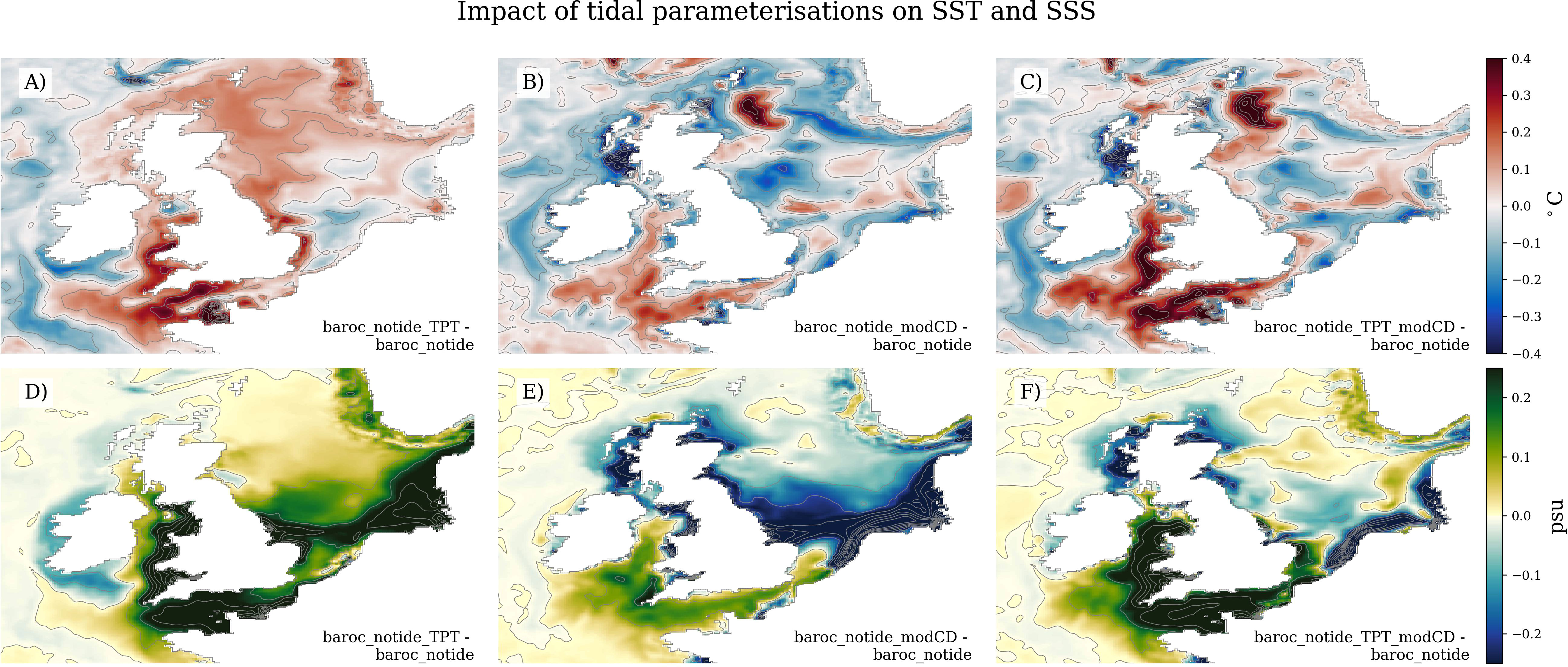
Figure 9 Impact of tidal parameterisation on the mean SST (A–C) and SSS (D–F). How the mean SST and SSS changes (relative to the baroc_notide) when applying: (A, D) the TPT parameterisation, (B, E) the modified bed drag coefficient, and (C, F), both.

Tinker and Hermanson (2021) showed that the GloSea5 SST and SSS predictability was much lower in the Irish Sea, Celtic Sea and the English Channel, in similar regions to the increased biases. We correlated the baroc_tide and baroc_notide SST and SSS for the 3 winter months of the 10 years of the simulations (giving 30 values; the 10 winter means gave similar patterns and values). SST correlations were high (>0.9) across the NWS, apart from the western Irish Sea, and the Celtic Sea and western English Channel to a lesser extent (Supplementary Material Figure 12). Salinity correlations were lower across the NWS, although most of the central and northern North Sea had correlations >0.8. The English Channel, Irish Sea, Celtic Sea and southern North Sea all had much lower correlations, (between 0 and 0.5). This region matches the region of low predictability identified by Tinker and Hermanson (2021), suggesting that the lack of tides in GloSea5 is partly causing the reduced predictability in this region.

The tidal parameterisations tend to improve these correlations. As the SST correlations were relatively high, the changes are relatively small (typically<0.05). The TPT parameterisation increases the SST correlations in the Irish Sea, and the western English Channel (Figure 10A). The drag coefficient parameterisation improves the SST correlation in the Irish Sea and southern North Sea (Figure 10B). Again, these improvements approximately combine when both parameterisations are included (Figure 10C). The improvements in the salinity correlations are much greater. TPT parameterisation increases the SSS correlations in the Irish Sea, and the western English Channel by ~0.3, effectively removing this low predictability region (Figure 10D). The drag coefficient parameterisation also improves the Irish Sea correlations, but not those in the English Channel (Figure 10E). The southern North Sea is not improved by any of the parameterisations (Figures 10D–F).

FIGURE 10

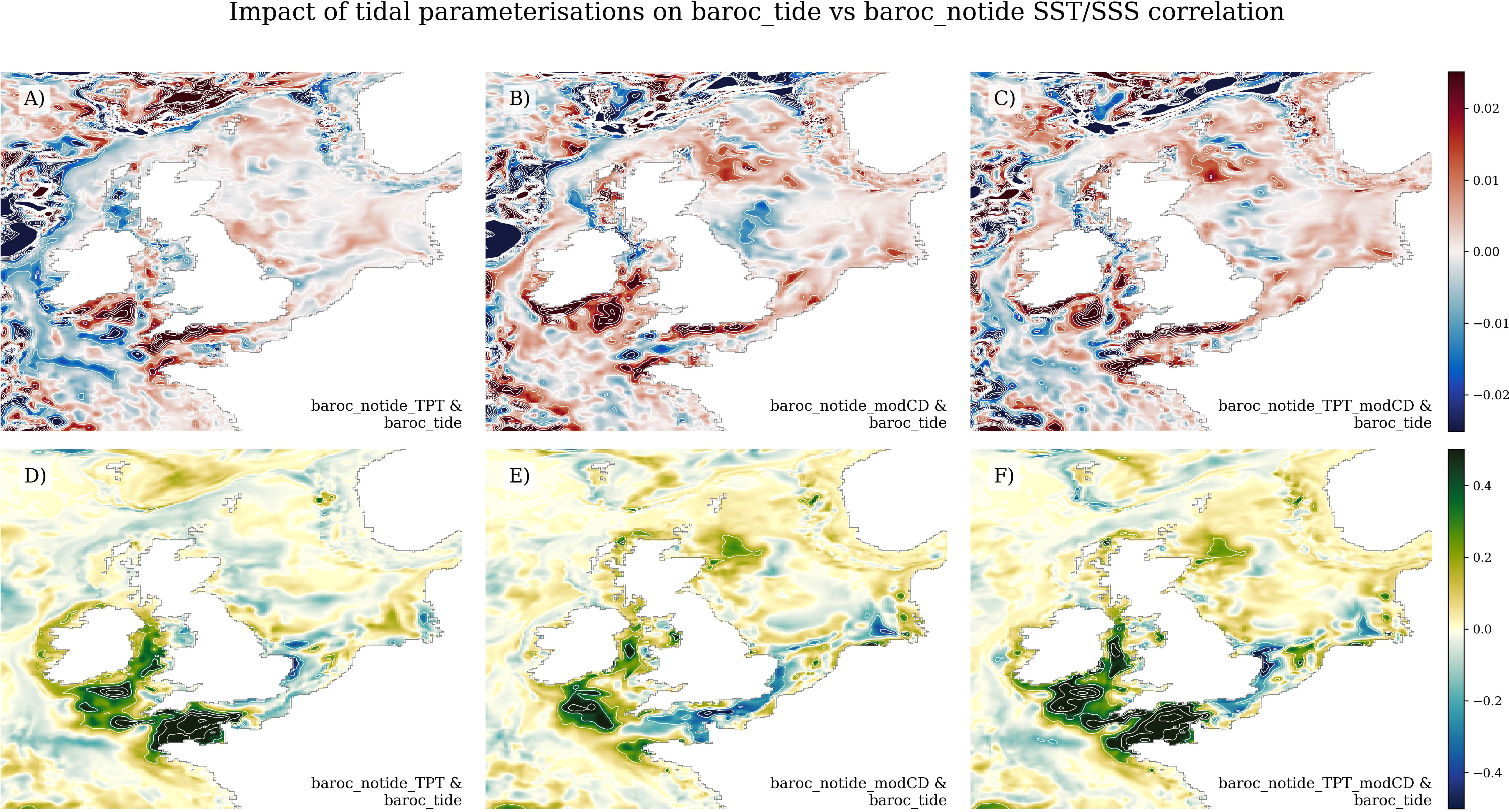
Figure 10 Impact of tidal parameterisation on the SST (A–C) and SSS (D–F) predictability. The temporal correlation between the winter SST and SSS (from 3 month for each of the 10 years) between baroc_tide and baroc_notide show how much the tides could affect predictability (Supplementary Material Figure 12). Here we show how that correlation is improved when we apply the tidal parameterisation: (A, D) the TPT parameterisation, (B, E) the modified bed drag coefficient, and (C, F), both. Positive numbers show an improvement.

So, while the TPT parameterisation does not improve the residual circulation, it plays an important role in improving the representation of the temperature and salinity fields, both in terms of the climatological mean, but also in the predictability.

4 Discussion

Residual currents can be produced by wind drag on the sea surface, wave-current interactions or driven by lateral density gradients due to non-uniform salinity or temperature distributions. However, they can also be generated by the tidal flow itself – the non-linear interactions of the oscillating tidal streams can lead to residual flows (Robinson, 1983).

While tidally driven residuals may be weaker than storm-driven residual circulation, they can contribute to the overall long-term distribution and transport of water properties (Robinson, 1983). There are several mechanisms that can allow the tides to influence the residual flow: topographically driven residual eddies, e.g. near headlands and islands (Pingree and Griffiths, 1987), circulation around sandbanks (Huthnance, 1973) and basin eddies, can lead to localised differences in the flood and ebb circulation patterns that do not average out over the tidal cycle (Robinson, 1983). These tend to be local in scope, though if connected they may be significant over the NWS, but would require models of kilometric scale resolution (Polton, 2015).

A larger scale influence of tides on residual circulation over the NWS can be conceptualised by considering tidal energy propagating onto the shelf from the Atlantic and being largely dissipated through bed friction. Due to tidal interaction with bathymetry and coastlines (and bed features), this dissipation is not uniform in space or time. The differential dissipation sets up a non-uniform mean sea surface elevation pattern, which drives the residual circulation.

We have shown that the absence of tides in an ocean model affects the simulated average depth-mean winter residual circulation, as well as its inter-annual variability. While the transport (through cross-sections) is not significantly different between our ‘with tides’ and ‘without tides’ simulations, the tide drives significant differences in the temperature and salinity fields. We found that tides tended to reduce the mean flow over most of the NWS, with some localised increases, and propose two mechanisms: (1) a Tidal Phase-driven Transport (TPT) mechanism, and (2) a modified bed drag coefficient. We also note that energy can transfer between the tides and the residual flow (following Nihoul, 1980) – we explore this in the supplementary materials, but do not parameterise it, or include it in the main body of the paper.

When the peak tidal current occurs towards high and low tide (i.e. the tidal wave is a progressive wave, Ward et al., 2018), there is a greater mass transport in one direction than the other. Applying the concept of the “bolus” transport (Rhines, 1982; McDougall, 1991; Marshall, 1997) and averaging this mass flux over a tidal cycle leads to a net transport which is the basis of our TPT parameterisation. When the tidal wave is acting as a standing wave, the slack water occurs at high and low water, and so there is zero mass transport. This explains the low mass transport fluxes in Figure 5A that coincide with the standing waves in Supplementary Material Figure 5.

The increased near-bed velocities associated with tides lead to greater bed stresses and a reduced residual flow (both the mean and its inter-annual variability). By balancing the bed stresses when explicitly including the tide, we have created a modified bed drag coefficient that can be parameterised to simulate the effect of the tidally driven bed stress. By applying both parameterisations into NEMO CO6, we can simulate the effect that tides have on the residual circulation. Although these tide-parameterisations are both proof of concept (requiring additional testing and development), we demonstrate their impact on SST and SSS (see Figure 9).

The TPT parameterisation has been developed for the M₂ tidal constituent. Initial tests suggest that adding the fluxes of the other 14 tidal constituents (that are included in NEMO CO6) has little effect, but this requires further testing. Our parameterisation substantially strengthens the shelf break current, even though the TPT fluxes are relatively weak there. There are many approaches to add the calculated TPT fluxes to the NEMO modelled velocities. For example, the model velocities could be nudged towards the TPT velocities, or they could be combined with the modelled velocities within the advection scheme. Here we take a simple approach by computing the TPT fluxes and incorporating them into the momentum equations as an external force (by taking the vector cross product with the Coriolis vector). However, this approach only approximately replicates the calculated TPT fluxes (i.e. Figures 5A, B differ) - since the approach is merely being explored as a proof of concept we do not try to rectify this. Other approaches to calculate the TPT fluxes (e.g. analytic expression following Soulsby (1983), with depth varying information) and to incorporate them into the momentum equations (e.g. nudging) may improve the performance of this parameterisation.

In our modified bed drag coefficient parameterisation, we modify the drag coefficient to balance the bed stress in baroc_tide and baroc_notide. However, when we run NEMO with this parameterisation (baroc_notide_modCD) we do not recover the baroc_tide bed stresses. This is because there is an iterative process: 1) we increase the bed drag coefficient in baroc_notide_modCD so its bed stress matches baroc_tide; 2) the increased bed stresses reduce the bed velocities; 3) this reduces the bed stresses. In order to fix the bed stresses in the non-tidal model to that of baroc_tide, a more sophisticated, interactive approach may be needed.

Our study builds on the work of Tinker and Hermanson (2021) who first showed the incorrect southward Irish Sea transport in a non-tidal ocean model (NEMO ORCA025 within GloSea5). As well as the lack of tides, reduced resolution etc., GloSea5 poorly resolved the details of the density field, which could degrade its representation of baroclinic transport processes. This could help explain why we still show northward transport across the Irish Sea in baroc_notide. We briefly consider the Irish Sea baroclinic transport with an additional pair of barotropic simulations, with and without tides (barot_tide and barot_notide) in Supplementary Material section 13.3. We find a strong southward Irish Sea transport in the barotropic simulations (0.4 and 0.9 Sv for barot_tide and barot_notide respectively (c.f. the northward transport of baroc_tide and baroc_notide of ~0.25 Sv and 0.2 Sv respectively Table 2) which suggests there is a northward baroclinic component to the Irish Sea transport. This could be poorly resolved in GloSea5 and would exacerbate the southward transport. The differences in circulation between baroc_tide and barot_tide (Supplementary Material Figure 14F, Supplementary Material Figure 15F) has implications for barotropic simulations of the NWS (e.g. Chen et al., 2014; O’Neill et al., 2016), we suggest that the relevance of these implications should be considered for each application.

We have focused on the winter season when most of the NWS is fully mixed, and so the baroclinic circulation is likely to be at a minimum. However, wind stress magnitude is also likely to be at a maximum during the winter period. In other seasons, tidal mixing fronts drive a series of seasonal jets, which form an important part of the summer residual circulation. When considering transport pathways and connectivity issues, seasonality effects (e.g. Mayorga-Adame et al., 2022) may dominate over the tidal residual circulation mechanism considered here. They are also likely to be poorly simulated in non-tidal global circulation models, and may require additional parameterisations. While we consider this out of scope for the current paper, we suggest additional research to investigate how the role of the tide in driving the residual circulation varies with season, and to identify and parameterise the additional processes.

The current generation of CMIP6 global climate models do not simulate tides, and our result shows the absence of tides within GloSea5 degrade the circulation, and so temperature and salinity distribution. We have also found similar circulation (and temperature and salinity) errors when assessing CMIP6 models based on ORCA025 (HadGEM3-GC31-MM, CMCC-CM2-HR4, CNRM-CM6), and a HadGEM3 GC3.0 present day control simulation (used to drive Tinker et al., 2020) against the CMEMS NWS reanalysis. When downscaling Tinker et al. (2020) with NEMO CO6 (as used in this study), the errors in the circulation (and temperature and salinity) improved in a similar manner to Tinker and Hermanson (2021).

We recommend our proof-of-concept parameterisation should be applied to help improve climate model simulation of the global shelf seas regions: for example, improving the representation of advective pathways in tidal regions could improve the future changes to distribution of tracers (including temperature, salinity, pollution, sediments and nutrients) and their temporal variability – our experiments suggest this could reduce GCM biases and increase model realism and skill. Current GCM simulation of the NWS makes it difficult to use GCM model output directly for impact studies in this region – we hope our parameterisation may allow some impact studies to use GCM data without needing costly dynamic downscaling.

In our study we can prove that the residual circulation changes when the tides are omitted, and the Irish Sea, Celtic Sea and English Channel become colder and fresher. We hypothesise that they become fresher/colder because more of the water is coming down through the Irish Sea (rather from the Atlantic across the Celtic Sea, as supported by circulation maps), but we do not prove it. The Irish Sea volume transport cross-sections could have clearly shown this circulation pathway, but the modelled difference is relatively small (and much smaller the inter-annual variability, Figure 3) – such a pathway could be obscured by other currents passing through the cross-section, as shown in Figure 1. So, while the currents and temperatures and salinity all respond to the tides in a coherent manner that suggests an Irish Sea transport pathway, we can link the two anecdotally, but can’t prove the link. This isn’t crucial for our study, but it would be an interesting finding. A connectivity matrix could be made for each simulation, by running a particle tracking programme, and seeing the proportion of particles that pass through the North Channel and Dover Strait. This may confirm the hypothesis that more of the English Channel water passes through the Irish Sea without tides.

We believe that our parameterisations may improve the simulation of shelf seas regions by non-tidal GCMs, although additional research is required. We did not explore other seasons, which will have other mechanisms (including those related to tidal mixing fronts) that may need to be parameterised. Our proof-of-concept parameterisations needs further development and testing, both within NWS models, and within global models. We have focused on the NWS – the residual circulation of other shelf seas around the world are likely to be similarly affected by tides. These regions need to be identified by comparing a global tidal and non-tidal model. Global fields for the TPT fluxes and modified bed drag coefficient need to be calculated, from a global tidal analysis and a pair of global tidal and non-tidal model respectively. It may be possible to apply these parameterisations locally within the global model (e.g. by only modifying the bed drag coefficient on the NWS), or even during certain seasons. If we can improve the residual circulation of shelf and tidal regions across the globe, we may be able to improve temperature and salinity biases and correlations, as suggested by Tinker and Hermanson (2021), which would make GCM’s much more useful to end users in many regions around the world.

5 Conclusions

Our comparison of NWS model simulations with and without tides has shown that:

• Excluding tides can affect the residual circulation.

• This can lead to differences in the mean distribution of temperature and salinity, and their temporal evolution (variability).

In order to explain how tides affect the residual circulation, and to explore whether they can be parameterised:

• We have identified two tidal mechanisms that impact the residual circulation:

– Tidal Phase-driven Transport (TPT); and

– the modified bed drag coefficient.

• We have implemented them within our model, and shown that they improve the NWS residual circulation, temperature and salinity biases and representation of variability.

This suggests our proof-of-concept parameterisations can simulate the impact tides have on residual circulation. If our approach can be included in global ocean and climate models, we may be able to improve the representation of residual circulation in tidal regions, and their distribution and variability of tracers (including temperature, salinity and nutrients), as suggested by Tinker and Hermanson (2021). This could allow some NWS impact studies to be based directly on GCM data, without the need for costly dynamic downscaling, making GCM data much more useful to end users in many regions around the world.

Data availability statement

The raw data supporting the conclusions of this article will be made available by the authors, without undue reservation.

Author contributions

JT designed the methodology, ran the simulations, analysed the results, prepared the initial manuscript, and developed the current uncertainty ellipse methodology. JT, JP, PR, and ML explored tidal processes. JT, JP, and PR developed the tidal parameterisations. JP developed the theoretical basis for the parameterisations. CO undertook the initial barotropic tidal simulations. All contributed to the final manuscript.

Acknowledgments

JT was supported by the Met Office Hadley Centre Climate Programme funded by BEIS and Defra. JP contribution was facilitated by the Joint Marine Modelling Project and supported by the “Climate Linked Atlantic Sector Science” (CLASS; NERC Marine National Capability) project. PR’s time was supported by the NERC projects NE/V004239/1 and NE/W001217/1. ML wishes to acknowledge the EPSRC METRIC project (EP/R034664/1) and the SEEC project (part funded by the European Regional Development Fund). The authors would like to thank the reviewers for their time and insights. They have led to a stronger paper. This paper is dedicated to Tristan Terence Wairua Tinker Vega, who was born during the final review of this paper. Terence was Tristan’s late grandfather (who died at 31), and Wairua is Māori for the spirit, or a soulful person. It also directly translates at two waters, reflecting his Pacific and Mediterranean origins.

Conflict of interest

The authors declare that the research was conducted in the absence of any commercial or financial relationships that could be construed as a potential conflict of interest.

Publisher’s note

All claims expressed in this article are solely those of the authors and do not necessarily represent those of their affiliated organizations, or those of the publisher, the editors and the reviewers. Any product that may be evaluated in this article, or claim that may be made by its manufacturer, is not guaranteed or endorsed by the publisher.

Supplementary material

The Supplementary Material for this article can be found online at: https://www.frontiersin.org/articles/10.3389/fmars.2022.847138/full#supplementary-material

Footnotes

1. ^ CMEMS product code: NORTHWESTSHELF_REANALYSIS_PHY_PHY_004_009

References

Chen X., Dangendorf S., Narayan N., O’Driscoll K., Tsimplis M. N., Su J., et al. (2014). On sea level change in the north Sea influenced by the north Atlantic oscillation: Local and remote steric effects. Estuarine Coast. Shelf Sci. 151, 186–195. doi: 10.1016/j.ecss.2014.10.009

CrossRef Full Text | Google Scholar

Domingues C. M., Church J. A., White N. J., Gleckler P. J., Wijffels S. E., Barker P. M., et al. (2008). Improved estimates of upper-ocean warming and multi-decadal sea-level rise. Nature 453 (7198), 1090–10U6. doi: 10.1038/nature07080

PubMed Abstract | CrossRef Full Text | Google Scholar

Egbert G., Ray R. D. (2001). Estimates of M2 tidal energy dissipation from TOPEX/Poseidon altimeter data. J. Geophys. Res. 106 (C10), 22475–22502. doi: 10.1029/2000JC000699

CrossRef Full Text | Google Scholar

Flather R. A. (1981). “Results from a model of the north-east Atlantic relating to the Norwegian coastal current,” in The Norwegian coastal current. Eds. Sætre R., Mork M.(Bergen:University of Bergin, Norway).

Google Scholar

Hermans T. H. J., Tinker J., Palmer M. D., Katsman C. A., Vermeersen B. L. A., Slangen A. B. A. (2020). Improving sea-level projections on the northwestern European shelf using dynamical downscaling. Climate Dynamics 54 (3–4), 1987–2011. doi: 10.1007/s00382-019-05104-5

CrossRef Full Text | Google Scholar

Hill A. E., Brown J., Fernand L., Holt J., Horsburgh K. J., Proctor R., et al. (2008). Thermohaline circulation of shallow tidal seas. Geophys. Res. Lett. 35 (11), L11605. doi: 10.1029/2008gl033459

CrossRef Full Text | Google Scholar

Hughes G. B., Chraibi M. (2012). Calculating ellipse overlap areas. Computing Visualization Sci. 15, 291–301. doi: 10.1007/s00791-013-0214-3

CrossRef Full Text | Google Scholar

Huthnance J. (1973). Tidal current asymmetries over the Norfolk sandbanks. Estuar. Coast. Mar. Sci. 1, 89–99. doi: 10.1016/0302-3524(73)90061-3

CrossRef Full Text | Google Scholar

Huthnance J. (1984). Slope currents and “JEBAR”. J. Phys. Oceanography 14, 795–810. doi: 10.1175/1520-0485(1984)014<0795:SCA>2.0.CO;2

CrossRef Full Text | Google Scholar

Inman H. F., Bradley E. L. (1989). The overlapping coefficient as a measure of agreement between probability distributions and point estimation of the overlap of two normal densities. Commun. Stat. - Theory Methods 18 (10), 3851–3874. doi: 10.1080/03610928908830127

CrossRef Full Text | Google Scholar

King N. G., Wilmes S. B., Smyth D., Tinker J., Robins P. E., Thorpe J., et al. (2021). Climate change accelerates range expansion of the invasive non-native species, the pacific oyster, crassostrea gigas. ICES J. Mar. Sci. 78 (1), 70–81. doi: 10.1093/icesjms/fsaa189

CrossRef Full Text | Google Scholar

Laurindo L. C., Mariano A. J., Lumpkin R. (2017). An improved near-surface velocity climatology for the global ocean from drifter observations. Deep Sea Res. Part I: Oceanographic Res. Papers 124, 73–92. doi: 10.1016/j.dsr.2017.04.009

CrossRef Full Text | Google Scholar

MacLachlan C., Arribas A., Peterson K. A., Maidens A., Fereday D., Scaife A. A., et al. (2014). Global seasonal forecast system version 5 (GloSea5): a high-resolution seasonal forecast system. Q. J. R. Meteorological Soc. 141 (689), 1072–1084. doi: 10.1002/qj.2396

CrossRef Full Text | Google Scholar

Madec G., Delecluse P., Imbard M., Levy C. (2016). OPA 8 Ocean General Circulation Model Technical report (Note Du Pôle de Modélisation). doi: 10.1016/j.joms.2014.06.438

CrossRef Full Text | Google Scholar

Marshall D. (1997). Subduction of water masses in an eddying ocean. J. Mar. Res. 55 (2), 201–222. doi: 10.1357/0022240973224373

CrossRef Full Text | Google Scholar

Mayorga-Adame C. G., Polton J. A., Fox A., Henry L.-A. (2022). Spatiotemporal scales of larval dispersal and connectivity among oil and gas structures in the north Sea. Mar. Ecol. Prog. Ser. 685, 49–67. doi: 10.3354/meps13970

CrossRef Full Text | Google Scholar

McDougall T. J. (1991). Parameterizing mixing in inverse models. Dynamics of Oceanic Internal Gravity Waves: Proc. ‘Aha Huliko ‘a Hawaiian Winter Workshop. 355–386.

Google Scholar

Nagy H., Pereiro D., Yamanaka T., Cusack C., Nolan G., Tinker J., et al. (2021). The Irish Atlantic CoCliME case study configuration, validation and application of a downscaled ROMS ocean climate model off SW Ireland. Harmful Algae. 107, 102053. doi: 10.1016/j.hal.2021.102053

PubMed Abstract | CrossRef Full Text | Google Scholar

Nihoul J. C. J. (1980). Residual circulation, long waves and mesoscale eddies in the north Sea. Oceanologica Acta 3 (3), 309–316.

Google Scholar

Nihoul J. C. J., Ronday F. C. (1975). The influence of the “tidal stress” on the residual circulation: application to the southern bight of the north Sea. Tellus 27 (5), 484–490. doi: 10.3402/tellusa.v27i5.10174

CrossRef Full Text | Google Scholar

O’Dea E., Furner R., Wakelin S., Siddorn J., While J., Sykes P., et al. (2017). The CO5 configuration of the 7 km Atlantic margin model: large-scale biases and sensitivity to forcing, physics options and vertical resolution. Geosci. Model. Dev. 10, 2947–2969. doi: 10.5194/gmd-10-2947-2017

CrossRef Full Text | Google Scholar

O’Neill C., Saulter A., Williams J., Horsburgh K. (2016). NEMO-surge: Application of atmospheric forcing and surge evaluation: Weather science technical report 619 (Exeter:Met Office, Exeter, UK). Available at: https://digital.nmla.metoffice.gov.uk/IO_53fa4f69-432c-40bb-9481-8c7dfbd6492d/.

Google Scholar

Piano M., Neill S. P., Lewis M. J., Robins P. E., Hashemi M. R., Davies A. G., et al. (2017). Tidal stream resource assessment uncertainty due to flow asymmetry and turbine yaw misalignment. Renewable Energy 114 (Part B), 1363–1375. doi: 10.1016/j.renene.2017.05.023

CrossRef Full Text | Google Scholar

Pingree R. D., Griffiths D. K. (1979). Sand transport paths around the British isles resulting from m 2 and m 4 tidal interactions. J. Mar. Biol. Assoc. United Kingdom 59 (2), 497–513. doi: 10.1017/S0025315400042806

CrossRef Full Text | Google Scholar

Pingree R. D., Griffiths D. K. (1987). Tidal friction for semidiurnal tides. Continental Shelf Res. 7 (10), 1181–1209. doi: 10.1016/0278-4343(87)90084-7

CrossRef Full Text | Google Scholar

Polton J. A. (2015). Tidally induced mean flow over bathymetric features: a contemporary challenge for high-resolution wide-area models. Geophys. Astrophysical Fluid Dynamics. 109 (3), 207–215. doi: 10.1080/03091929.2014.952726

CrossRef Full Text | Google Scholar

Polton J. A., Lewis D. M., Belcher S. E. (2005). The role of wave-induced Coriolis-stokes forcing on the wind-driven mixed layer. J. Phys. Oceanography. 35 (4), 444–457. doi: 10.1175/JPO2701.1

CrossRef Full Text | Google Scholar

Prandle D. (1997). Tidal currents in shelf seas - their nature and impacts. Prog. Oceanography. 40 (1–4), 245–261.doi: 10.1016/S0079-6611(98)00013-5

CrossRef Full Text | Google Scholar

Pugh D. (1987). Tides, surges and mean sea-level (Chichester: John Wiley and Sons).

Google Scholar

Renshaw R., Wakelin S. L., Mahdon R., O’Dea E., Tinker J. (2019). Copernicus Marine environment monitoring service quality information document north West European shelf production centre NORTHWESTSHELF_REANALYSIS_PHYS_004_009 Copernicus Marine Environmental Monitoring Service, Toulouse, France). Available at: http://marine.copernicus.eu/documents/QUID/CMEMS-NWS-QUID-004-009.pdf.

Google Scholar

Rhines P. B. (1982). Basic dynamics of the large-scale geostrophic circulation (Summer Study Program in Geophysical Fluid Dynamics, Woods Hole Oceanographic Institution).

Google Scholar

Robins P. E., Neill S. P., Lewis M. J., Ward S. L. (2015). Characterising the spatial and temporal variability of the tidal-stream energy resource over the northwest European shelf seas. Appl. Energy. 147, 510–522. doi: 10.1016/j.apenergy.2015.03.045

CrossRef Full Text | Google Scholar

Robinson I. S. (1983). Tidally induced residual flows. Elsevier Oceanography Ser. 35, 321–356. doi: 10.1016/S0422-9894(08)70505-1

CrossRef Full Text | Google Scholar

Siddorn J. R. R., Furner R. (2013). An analytical stretching function that combines the best attributes of geopotential and terrain-following vertical coordinates. Ocean Model. 66, 1–13. doi: 10.1016/j.ocemod.2013.02.001

CrossRef Full Text | Google Scholar

Simpson J. H. (1997). Physical processes in the ROFI regime. J. Mar. Syst. 2 (1–4), 3–15. doi: 10.1016/S0924-7963(96)00085-1

CrossRef Full Text | Google Scholar

Simpson J. H., Allen C. M., Morris N. C. G. (1978). Fronts on the continental shelf. J. Geophys. Res. 83 (C9), 4607. doi: 10.1029/JC083iC09p04607

CrossRef Full Text | Google Scholar

Small C., Nicholls R. J. (2003). A global analysis of human settlement in coastal zones. J. Coast. Res. 584–599. Available at: http://www.jstor.org/stable/4299200

Google Scholar

Soulsby R. L. (1983). Chapter 5 The Bottom Boundary Layer of Shelf Seas. in: Elsevier Oceanography Series 189–266, doi: 10.1016/S0422-9894(08)70503-8.

CrossRef Full Text | Google Scholar

Stokes G. G. (1847). On the theory of oscillatory waves. Trans. Cambridge Philos. Soc. 8, 441. doi: 10.1017/cbo9780511702242.013

CrossRef Full Text | Google Scholar

Storkey D., Blaker A. T., Mathiot P., Megann A., Aksenov Y., Blockley E. W., et al. (2018). UK Global ocean GO6 and GO7: a traceable hierarchy of model resolutions. Geoscientific Model. Dev. 11 (8), 3187–3213. doi: 10.5194/gmd-11-3187-2018

CrossRef Full Text | Google Scholar

Tinker J., Hermanson L. (2021). Towards winter seasonal predictability on the north West European shelf seas. Front. Mar. Sci. 8. doi: 10.3389/fmars.2021.698997

PubMed Abstract | CrossRef Full Text | Google Scholar

Tinker J., Krijnen J., Wood R., Barciela R., Dye S. R. (2018). What are the prospects for seasonal prediction of the marine environment of the north-west European shelf? Ocean Sci. 14 (4), 887–909. doi: 10.5194/os-14-887-2018

CrossRef Full Text | Google Scholar

Tinker J., Lowe J., Pardaens A., Holt J., Barciela R. (2016). Uncertainty in climate projections for the 21st century northwest European shelf seas. Prog. In Oceanography 148, 56–73. doi: 10.1016/j.pocean.2016.09.003

CrossRef Full Text | Google Scholar

Tinker J., Palmer M. D., Copsey D., Howard T. P., Lowe J., Hermans T. H. J. (2020). Dynamical downscaling of unforced interannual sea-level variability in the North-West European shelf seas. Climate Dynamics. 55, 2207–2236. doi: 10.1007/s00382-020-05378-0

CrossRef Full Text | Google Scholar

Tinker J., Polton J. A. (2022). hadjt/CurrUncertEllipses: v0.0.0. zenodo. doi: 10.5281/zenodo.6482468

CrossRef Full Text | Google Scholar

Townhill B., Pinnegar J., Tinker J., Jones M., Simpson S., Stebbing P., et al. (2017). Non-native marine species in north-west Europe: Developing an approach to assess future spread using regional downscaled climate projections. Aquat. Conservation: Mar. Freshw. Ecosyst. 27 (5), 1035–1050. doi: 10.1002/aqc.2764.

CrossRef Full Text | Google Scholar

Wakelin S. L., Holt J. T., Proctor R. (2009). The influence of initial conditions and open boundary conditions on shelf circulation in a 3D ocean-shelf model of the north East Atlantic. Ocean Dynamics 59 (1), 67–81. doi: 10.1007/s10236-008-0164-3

CrossRef Full Text | Google Scholar

Ward S. L., Robins P. E., Lewis M. J., Iglesias G., Hashemi M. R., Neill S. P. (2018). Tidal stream resource characterisation in progressive versus standing wave systems. Appl. Energy. 220, 274–285. doi: 10.1016/j.apenergy.2018.03.059

CrossRef Full Text | Google Scholar

Williams K. D., Copsey D., Blockley E., Bodas-Salcedo A., Calvert D., Comer R. E., et al. (2018). The met office global coupled model 3.0 and 3.1 (GC3 & GC3.1) configurations. J. Adv. Model. Earth Syst. 10 (2), 357–380. doi: 10.1002/2017MS001115

CrossRef Full Text | Google Scholar

Williams K. D., Harris C. M., Bodas-Salcedo A., Camp J., Comer R. E., Copsey D., et al. (2015). The met office global coupled model 2.0 (GC2) configuration. Geoscientific Model. Dev. 8 (5), 1509–1524. doi: 10.5194/gmd-8-1509-2015

CrossRef Full Text | Google Scholar

Yool A., Fasham M. J. R. (2001). An examination of the “continental shelf pump” in an open ocean general circulation model. Global Biogeochemical Cycles 15 (4),831–844. doi: 10.1029/2000GB001359

CrossRef Full Text | Google Scholar