The Presence of a Substrate Strengthens The Jet Generated by Upside-Down Jellyfish

Upside-down jellyfish, Cassiopea, are prevalent in warm and shallow parts of the oceans throughout the world. They are unique among jellyfish in that they rest upside down against the substrate and extend their oral arms upwards. This configuration allows them to continually pull water along the substrate, through their oral arms, and up into the water column for feeding, nutrient and gas exchange, and waste removal. Although the hydrodynamics of the pulsation of jellyfish bells has been studied in many contexts, it is not clear how the presence or absence of the substrate alters the bulk flow patterns generated by Cassiopea medusae. In this paper, we use three-dimensional (3D) particle tracking velocimetry and 3D immersed boundary simulations to characterize the flow generated by upside-down jellyfish. In both cases, the oral arms are removed, which allows us to isolate the effect of the substrate. The experimental results are used to validate numerical simulations, and the numerical simulations show that the presence of the substrate enhances the generation of vortices, which in turn augments the upward velocities of the resulting jets. Furthermore, the presence of the substrate creates a flow pattern where the water volume within the bell is ejected with each pulse cycle. These results suggest that the positioning of the upside-down jellyfish such that its bell is pressed against the ocean floor is beneficial for augmenting vertical flow and increasing the volume of water sampled during each pulse.

1 Introduction

Jellyfish are well-known to use muscle contractions while swimming, generating water currents to facilitate feeding and nutrient exchange. Studies have analyzed the ability of jellyfish to drive fluid using pulsations of their bell in the context of both swimming and feeding behavior, often with the two coupled together (Colin and Costello, 2002a; Colin and Costello, 2002b). The upside-down jellyfish, Cassiopea, presents a model system in which feeding may be decoupled from swimming and examined individually. Cassiopea is a relatively sessile jellyfish that, while capable of swimming, prefers to spend most of its time resting against the seafloor, with its bell resting against the substrate and its appendages [the oral arms) facing upward into the fluid. Despite only occasionally swimming, bell pulsations are vital to Cassiopea medusae to drive fluid from the immediate environment around its feeding sites (Arai, 1997; Passano, 2004; Jantzen et al., 2010; Hamlet et al., 2011; Santhanakrishnan et al., 2012)]. As Cassiopea medusae inhabit sheltered marine environments where low flow rates are expected in the benthic boundary layer, pulsation-induced flows are particularly significant for feeding, nutrient and gas exchange, and excretory functions.

The pulsing cycle of Cassiopea is divided into three distinct phases: 1) active contraction, 2) passive expansion, and 3) a quiescent period before the next contraction. During contraction, the coronal muscles in the jellyfish’s bell are active, drawing in connected pinnate muscles as they contract. A starting vortex is formed during the contraction that enhances the flow towards the medusa (see Figure 1). Once the muscle activation has ceased, the extracellular matrix known as the mesoglea that surrounds the muscles and comprises much of the mass of the bell releases the stored elastic energy as the bell relaxes back to its resting configuration (Arai, 1997). During this expansion phase, an oppositely spinning stopping vortex is formed that interacts with the starting vortex to draw fluid upward and away from the medusa. Once the bell has completely relaxed and comes to rest, the bell remains in this state until the activation of the muscles initiates the next contraction cycle. We define the duty cycle as the fraction of the total cycle devoted to contracting.

FIGURE 1

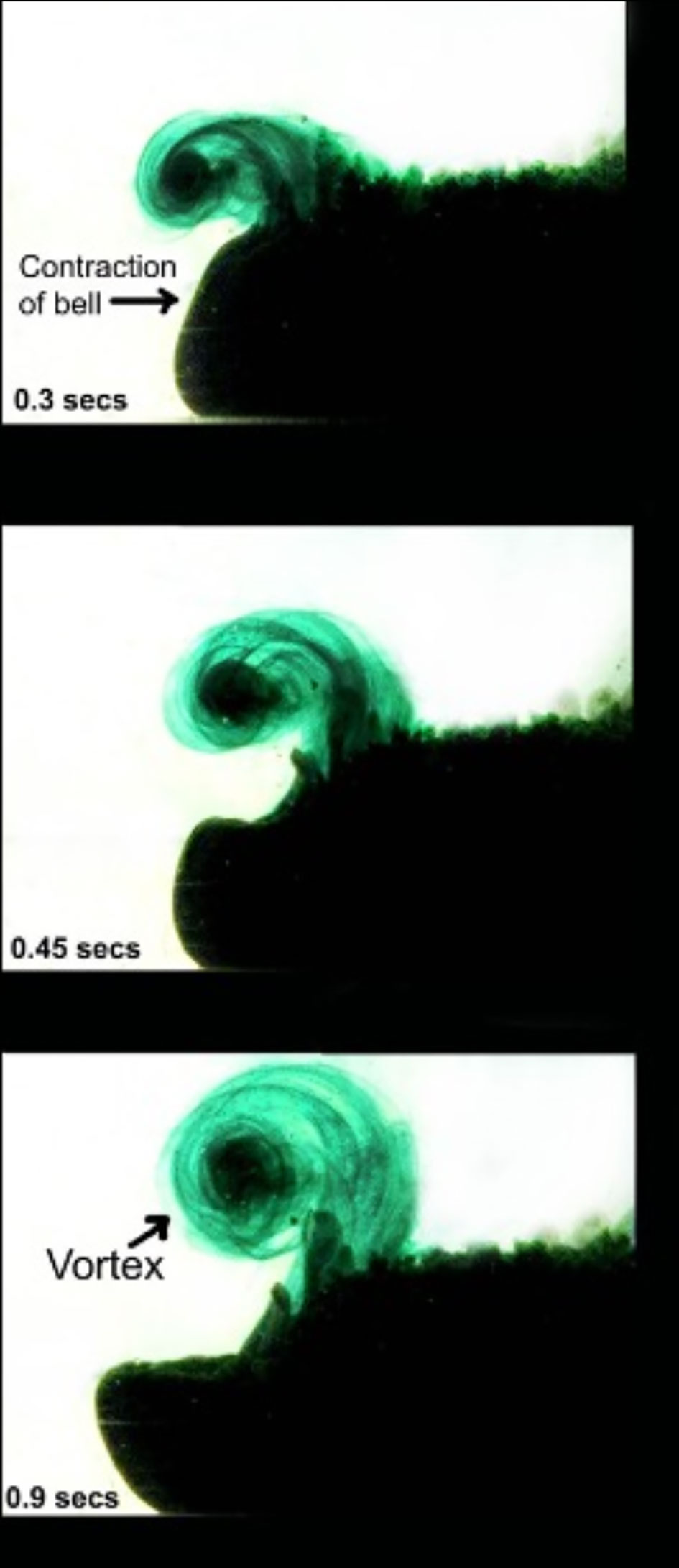
Figure 1 Dye visualization showing the formation and advection of the starting vortex after the jellyfish bell contracts. An oppositely spinning stopping vortex forms during the expansion of the bell (not shown).

Previous studies analyzed the fluid flow induced by the contracting bells of jellyfish experimentally (Santhanakrishnan et al., 2012; Durieux et al., 2021) and computationally (Hamlet et al., 2011; Hamlet and Miller, 2012). As mentioned above, Cassiopea offers an opportunity to examine fluid dynamics utilized for feeding uncoupled from swimming. These studies reveal that Cassiopea drives fluid towards the bell, through the oral arms, and upward and away from the medusa. This flow pattern is representative of a continuous upward jet that allows the medusa to sample new volumes of fluid with each pulse. In particular, there is little backflow in the radial direction during the expansion of the bell margin. Furthermore, the flow above the medusa moves continually upward, with the greatest magnitude of flow around the outer quarter of the oral arms. The medusa must reach a sufficiently high Reynolds number (Re) for this pattern to be established (Hamlet et al., 2011), and there is no obvious significant benefit to the jellyfish for pulsing in groups (Durieux et al., 2021). Furthermore, the presence of Cassiopea has been shown to enhance the release of nutrient-rich benthic porewater and promote water column mixing (Jantzen et al., 2010; Durieux et al., 2021).

One of the unique features of the upside-down jellyfish is that it is not typically found in open water but rests with its bell pressed against a substrate, such as the sandy ocean floor or the glass bottom of an aquarium. This provides an opportunity to study the effect of a wall on the flows driven by pulsing jellyfish bells. Despite extensive study of the fluid dynamics of currents generated by Cassiopea medusae, the role of the substrate in driving fluid has not been previously considered. We seek to address this point by examining the flow generated by the medusa with and without a substrate. Three-dimensional (3D) particle tracking velocimetry is used for the first time to resolve the 3D flow fields generated by a Cassiopea medusa resting on a sand bed (substrate) within an aquarium. Similarly, 3D numerical simulations using the immersed boundary method are used to quantify the flow fields generated by a simplified model of a Cassiopea medusa when the bell is rested against a smooth wall (substrate) and elevated above it.

The oral arms of both live and numerical medusae were removed to isolate the effect of the substrate on the flow around the jellyfish. Removal of the oral arms also simplifies the mathematical model and experimental measurements by eliminating the need to optically resolve or perform intensive 3D simulations of flow through the intricate details of the structures. It has been shown in two-dimensional simulations that the oral arms may serve to help direct the radial flow continually towards the medusa (Hamlet et al., 2011). It is also known that the oral arms generate additional drag (Katija, 2015) and break up the starting and stopping vortices into smaller vortical structures (Santhanakrishnan et al., 2012; Miles and Battista, 2019) which enhance mixing (Durieux et al., 2021). To our knowledge, this is the first study comparing experiments to computation in three dimensions that also considers the substrate’s effect.

2 Materials and Methods

2.1 Experimental Methods

2.1.1 Animal Care and Handling

Cassiopea medusae were purchased from Carolina Biological Supply Company (Burlington, NC, USA) during June 2020. These medusae were maintained in a home tank measuring 0.609 m × 0.609 m (24 in. × 24 in.) in cross-section that was filled with artificial seawater to a depth of 0.229 m (9 in.). The seawater was maintained at a temperature of 20-25°C using a submersible heater, and overhead metal halide lighting was turned on daily for 8 consecutive hours. Chemical parameters of the seawater were measured as follows: pH = 8.2, salinity = 1.225 g L^-1, and 0 ppm of ammonia, nitrate and nitrite. These animals were fed live brine shrimp (Artemia spp.) nauplii which were batch harvested using eggs purchased from Brine Shrimp Direct (Ogden, UT, USA). Animals were target fed once a week. To remove confounding effects of the oral arm network on the flow generated by bell pulsations, all oral arms were excised from an individual of 4 cm bell diameter (d, Figure 2A) using scissors. This individual was then transferred to a test aquarium measuring 0.609 m × 0.609 m (24 in. × 24 in.) in cross-section that was filled with artificial seawater from the home tank to a depth of 0.254 m (10 in.). Commercially available black substrate (CaribSea Instant Aquarium Tahitian Moon Reef & Marine Substrate, CaribSea Inc., FL, USA) was used to make a 1 cm sand bed in the test aquarium. All the experiments were conducted at room temperature (20-25°C) in July 2020.

FIGURE 2

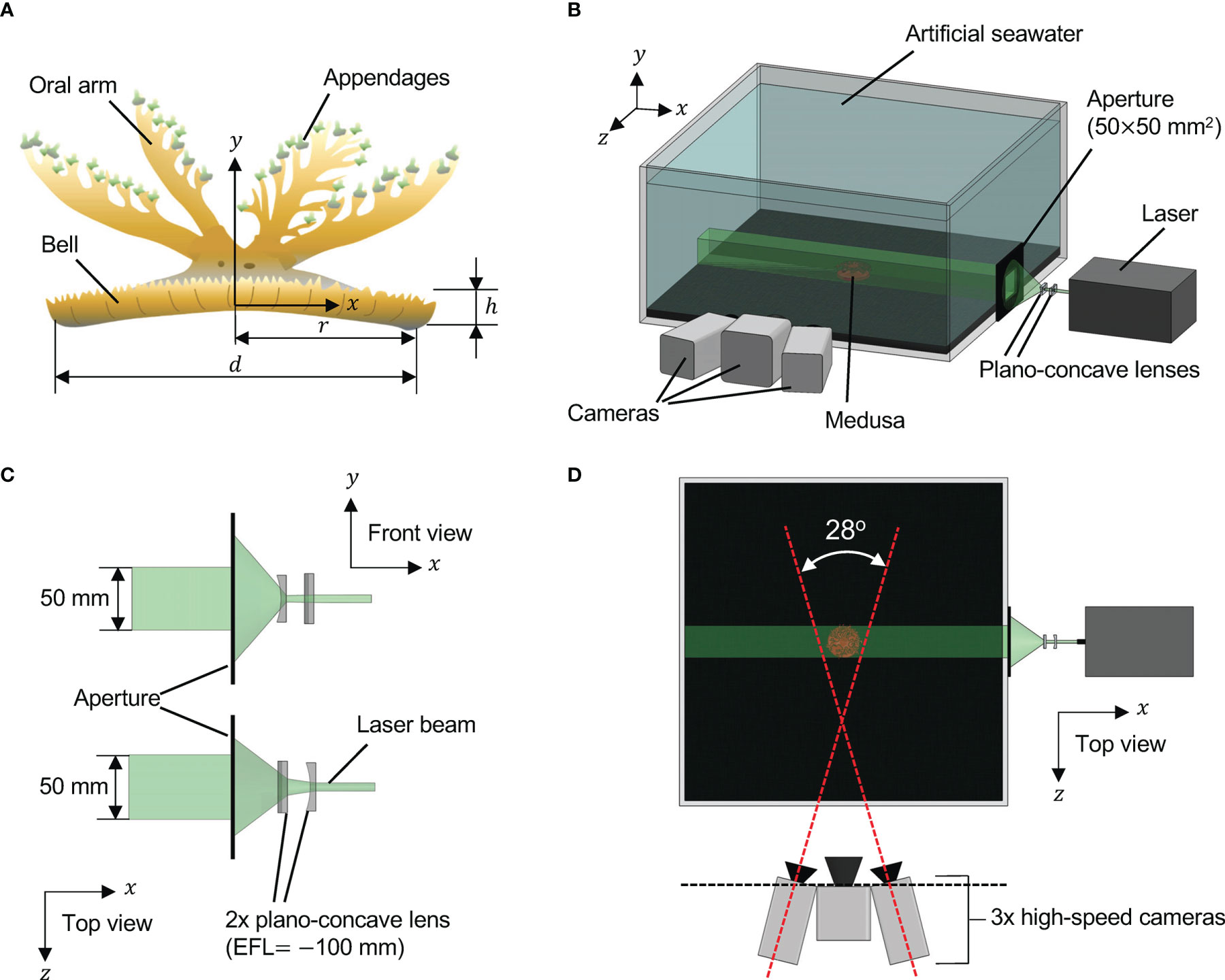
Figure 2 Experimental arrangements. (A) Morphology of Cassiopea spp. with oral-aboral axis at (x,z) = (0,0). d = bell diameter; r = bell radius (= d/2); h = bell height. (B) Three-dimensional (3D) particle tracking velocimetry (PTV) setup. A medusa with oral arms removed (d = 40 mm; h = 4 mm) was positioned centrally inside a 30 gallon test aquarium (0.609 m × 0.609 m in cross-section) containing artificial seawater. Coordinate system used for experimental data analysis is shown. (C) Magnified view of volume optics consisting of two plano-concave lenses oriented perpendicular to each other. Each lens had an effective focal length (EFL) of -100 mm. The laser illuminated volume was trimmed to a rectangular region using a custom-made aperture measuring 50 mm tall × 50 mm wide. (D) Top view of the 3D PTV setup showing the three high-speed cameras used for imaging, with two of the side cameras at 14° relative to x = 0 line.

2.1.2 Three-Dimensional Particle Tracking Velocimetry Measurements

To examine the 3D flow field generated by the medusa with no oral arms, we performed 3D PTV measurements using the shake-the-box (STB) technique (Schanz et al., 2013; Schanz et al., 2016). A single-cavity, Neodymium-doped yttrium lithium fluoride (Nd: YLF) high-speed laser (Photonics Industries International, Inc., Bohemia, NY, USA) was used for illumination, which provided a 0.5 mm diameter beam with wavelength of 527 nm. The beam was propagated through a combination of two cylindrical plano-concave lenses (each with effective focal length of -100 mm) oriented perpendicular to each other, in order to generate a conical illumination volume. This conical volume was next passed through a custom-made rectangular aperture with 50 mm x 50 mm opening to make a cuboidal illumination volume with sharp edges (Figures 2B, C). The cross-section of the illuminated field of view (FOV) was 50 mm in height and 50 mm in width, passing through the entire length of the test aquarium. Fluorescent particles of diameter ranging from 45-53 μm (specific gravity = 1.0) were used as tracers and homogeneously seeded in the test aquarium prior to introducing the medusa. The seeding density was estimated to be on the order of 0.01 particles per pixel. Three high-speed complementary metal–oxide–semiconductor (CMOS) cameras (2 Phantom M110 and 1 Phantom VEO 310L, Vision Research Inc., Wayne, NJ, USA) were used for acquiring raw images of tracer particles. Each M110 camera was oriented 14° relative to the centrally positioned VEO 310L camera (Figure 2D), such that the image plane of the VEO 310L was parallel to the lengthwise axis of the illumination volume. Each M110 camera was mounted with a Scheimpflug adapter (LaVision GmbH, Göttingen, Germany) to correct for off-axis viewing distortion and attached to a 100 mm focal length macro lens (AT-X M100 PRO D, Kenko Tokina Co., Ltd., Tokyo, Japan). The VEO 310L camera was attached to a 105 mm focal length macro lens (Nikon Micro-Nikkor, Nikon Corporation, Tokyo, Japan). All the camera lenses were attached to a 550 nm long-pass optical filter. DaVis 10.1.1 software (LaVision GmbH, Göttingen, Germany) was used for acquiring and processing raw images.

Following the volume self-calibration procedure (as described in the Supplementary Material), the medusa with no oral arms was introduced in the test aquarium and moved to be centrally located in the FOV. The medusa was allowed to acclimate for 30 minutes before starting the acquisition of 3D PTV measurements. Within this acclimation time period, bell pulsations of the medusa were observed to be similar in rhythm to those observed before the removal of oral arms. After 30 minutes, 1000 images were recorded at 500 frames per second. These recorded images were preprocessed in DaVis to remove the animal from the images, followed by visual improvement of particles in each frame. Preprocessing steps included time subtraction with Gaussian smoothing filter, normalizing with the local average, particle sharpening and intensity count amplification. These preprocessed images were processed using the STB algorithm in DaVis. The STB algorithm used a subset of the acquired time series of images to determine 3D particle trajectories using iterative particle reconstruction (Wieneke, 2012). These identified particle positions were next used to predict particle positions at subsequent time points. Predicted particle positions were optimized by ‘shaking’ the particles in 3D space, with an allowable triangulation error of 1.5-5 pixels. 3D particle tracks obtained from STB processing were subject to fine scale reconstruction for generating velocity vector fields. 3D velocity vector fields were exported as DAT files that were read in custom scripts written in MATLAB (The Mathworks, Inc., Natick, MA) for plotting velocity profiles and Tecplot 360 (Tecplot Inc., Bellevue, WA, USA) for calculating and visualizing isovorticity contours.

Recordings from the central Phantom VEO 310L camera were exported as videos in AVI format. The displacement of the left and right tips of the bell margin were tracked in these raw images using DLTdv7 software (Hedrick, 2008) in MATLAB. Horizontal (x) and vertical (y) displacement of the tip of the bell margin were non-dimensionalized using bell radius (r) and bell height (h), respectively, to extract time-variation of x/r and y/h across a pulsing cycle.

2.2 Computational Methods and Modeling

2.2.1 Immersed Boundary Method

Numerical simulations to determine the flows generated by an elastic jellyfish pulsing in a viscous fluid were conducted with the immersed boundary method (Peskin, 2002). The immersed boundary method is a numerical method that solves fully-coupled fluid-structure interaction problems. A deformable structure is immersed in a viscous, incompressible fluid governed by the Navier-Stokes equations. The immersed boundary method was initially developed to study flow through the human heart (Peskin, 2002) and has evolved to model a diverse range of biofluids problems, including flagellar motion, anguilliform locomotion, jellyfish swimming, foam development, cell division, cellular migration, and viscoelastic systems (Kim et al., 2010; Tytell et al., 2010; Rejniak, 2012; Thomases and Guy, 2019; Hoover et al., 2021). Details regarding the immersed boundary method are found in the Supplementary Material, including all relevant equations.

For this study, we used a hybrid finite difference-finite element version of the immersed boundary method (IBFE) (Griffith and Luo, 2017) in which the fluid domain is discretized using a finite difference approach, and the immersed boundary (e.g., the jellyfish) is discretized using finite elements. The numerical simulations were performed using an adaptive and parallelized version of the immersed boundary method, IBAMR (Griffith, 2014). The following outline describes the three-dimensional formulation of the immersed boundary method. For a full review of the method, see Peskin (2002) and Griffith and Patankar (2020).

2.2.2 Material Model

This section briefly describes the modeling of the forces driving the motion of the jellyfish bell in the numerical simulations. A Neo-Hookean material model is used to describe the elastic bell of the jellyfish. The bell motion is driven by applying active stress in the subumbrellar region of the bell. The active muscle stress that drives this motion is described as fiber-oriented stress, which is generated by an applied tension that simulates tension from contracting the coronal muscles of the jellyfish. An additional body force is applied to the bell base to maintain its initial position. Material model parameters are summarized in Table 1. The mathematical details of material modeling methods are found in the Supplementary Material, including all relevant equations. The elastic properties of the bell were chosen to be within the range of typical cnidarian mesoglea and has been used in previous simulations of jellyfish swimming (Hoover et al., 2021).

TABLE 1

Table 1 The material parameters for the upside-down jellyfish model.

2.2.3 Numerical Model

Here we briefly describe the key parameters, with a more detailed description of the numerical setup and convergence analysis described in the Supplementary Material. An upside-down jellyfish bell of 0.05 m in diameter was constructed as a flat plate representing the bottom and an elliptical section representing the bell margin (see Figure 3). This bell size is within the range of Cassiopea, and note that the model was not constructed specifically to match any particular medusa considered in the experiments. The domain of the simulation was a cube with a side length of 0.5 m with no-slip boundary conditions.

FIGURE 3

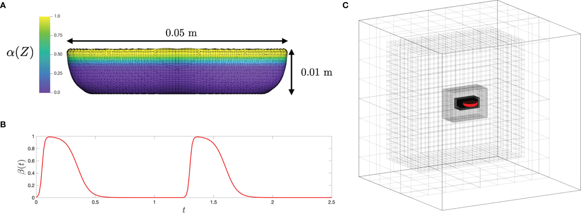
Figure 3 (A) The upside-down jellyfish model and mesh with α(Z) plotted on top; (B) a plot of β(t), the temporal parameterization of the activation and release of the active stress, with respect to time; and (C) the relative size of the fluid domain and positioning of the medusa, as well as the adaptive mesh refinement initialization.

The bell was driven at a frequency of 0.8 s^-1 through the periodic application of active tension along the bell margin that caused contraction of the bell. Note that the active tension models the action of the circumferential muscles rather than directly prescribing the bell’s motion. A similar approach has been used previously to model moon jellyfish (Aurelia aurita) swimming (Hoover et al., 2017; Hoover et al., 2019; Hoover et al., 2021). The maximum tension was set to 1000 N/m² and applied for 0.3 s at the beginning of each pulse. The expansion of the bell was due to its passive elastic properties. The numerical and physical parameters are summarized in Table 2. Note that the pulse period of 1.25 seconds is within the range measured for Cassiopea (Hamlet et al., 2011; Santhanakrishnan et al., 2012). The applied tension and contraction duration were tuned to generate a reasonable contraction amplitude of the bell and allow sufficient time for the bell to fully expand. Several applied tensions were considered and found to not significantly alter the resulting flow fields.

TABLE 2

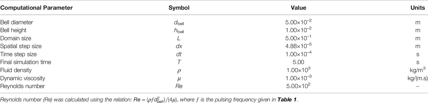
Table 2 The parameters for the numerical simulations of upside-down jellyfish.

We considered the first four pulse cycles of a numerical jellyfish that starts from rest. Note that in the experiment, there was a pause before the two cycles that were experimentally measured such that the fluid was nearly at rest near the jellyfish at the beginning of the first measured cycle. This is typical of Cassiopea who exhibit a large range of interpulse durations characterized by rest periods followed by a sequence of continuous pulses (Hamlet et al., 2012). The numerical simulation of four pulses from rest allows us to understand the development of the wake during such a sequence of pulses that follows a longer rest period.

3 Results

3.1 Bell Kinematics

3.1.1 Experimental Results

Kinematics of the bell margin tip were examined as a function of non-dimensional time (t/T), where t is dimensional time and T is the time period of the first bell pulsation cycle (T ≈ 1.18 s). During the power stroke (PS), the bell contracted with the tips of its margin moving toward the oral-aboral axis (x/r = 0). During the recovery stroke (RS), the bell expanded with the bell tip moving outward from oral-aboral axis. For the experimentally tested medusa with no oral arms (d = 4 cm), PS≈35% and RS≈65% in the first pulsing cycle.

After a short period of no x-displacement, the left tip of the bell margin contracted from a fully relaxed state (x/r = -1) in PS until x/r ≈ -0.5 (Figure 4A). The bell margin tip subsequently expanded toward the substrate in RS, starting from x/r ≈ -0.5 to x/r ≈ -1. The right tip of the bell margin displaced similar to the left side, contracting during PS from x/r = 1 to x/r = 0.5, and expanding during RS from x/r = 0.5 to x/r = 1. A small time-delay was observed between the left and right margin tips in early PS, suggesting that there was radial asymmetry in the bell motion. However, RS started at the same time on both sides of the bell margin.

FIGURE 4

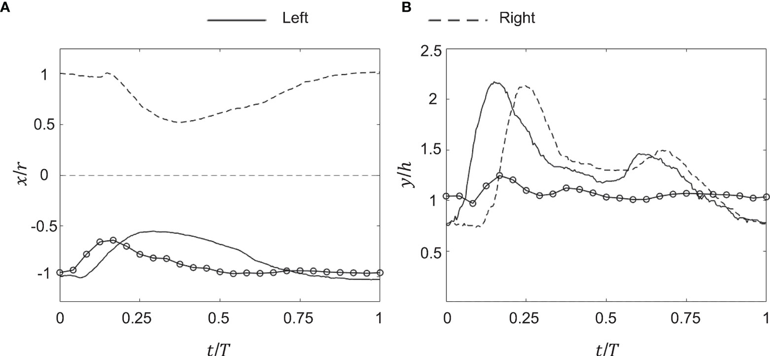
Figure 4 Kinematics of the medusa bell margin tip. (A) Non-dimensional horizontal displacement versus non-dimensional time (t/T). x/r is the ratio of bell margin tip displacement in the horizontal (x) direction to the bell radius (r). T is the time period of a bell pulsation cycle. (B) Non-dimensional vertical displacement versus t/T. y/h is the ratio of bell margin tip displacement in the vertical (y) direction to the bell height (h). Lines without markers correspond to experimental measurements on a live medusa, while lines with markers are from numerical simulations. Kinematics of the bell margin tip extracted from experimental data are shown for both the left side (solid lines) and right side (dashed lines), defined relative to the oral-aboral axis (x,z) = (0,0). Kinematics obtained from the numerical bell model were only tracked on the left side of the bell margin. r = 20 mm, h = 4 mm and T = 1.18 s were used to non-dimensionalize experimental data. r = 25 mm, h = 10 mm and T = 1.25 s were used to non-dimensionalize numerical data.

The left bell margin tip moved vertically upward during early PS (t/T ≈ 0.2) and decreased in height by the end of PS (t/T ≈ 0.35). The left bell margin tip increased in height from early RS to mid RS (t/T = 0.7) and finally decreased to fully relaxed state (y/h = 1) at the end of RS (t/T = 1). The right bell margin tip increased in height starting from t/T = 0.1 until t/T = 0.25, and subsequently decreased until t/T = 0.4. With increasing time, the right bell margin tip increased in height until t/T = 0.7 and later decreased in height to its relaxed state of y/h = 1 at t/T = 1. Similar to horizontal displacement (x/r) profiles, vertical displacement profiles showed a time delay between the left and right bell margin tips (compare Figures 4A, B).

3.1.2 Computational Results

Bell motion of the numerical jellyfish model was not prescribed, but rather realized via prescribing the active tension along the bell margin. Kinematics of the left tip of the bell margin were tracked from numerical simulations using DLTdv7 software (Hedrick, 2008) in MATLAB. Numerical bell kinematics were examined using the same non-dimensional displacement profiles as the experimental measurements. The bell margin tip moved radially inward in PS, reaching peak value at t/T ≈ 0.2 and subsequently moving outward until the end of PS (Figure 4A). The bell margin tip expanded radially outward during most of the RS. After a short period of negligible vertical (y) displacement, the numerical bell increased in height in early PS and subsequently decreased in height in late PS (Figure 4B). The left bell margin tip increased in height from early RS to mid RS and decreased in height toward the end of RS.

Time-variation of horizontal and vertical displacements of the numerical bell were qualitatively similar in trend to those extracted from experimental data. Phase offsets between experimental and numerical kinematics were likely due to using different pulsing cycle durations to non-dimensionalize t (T = 1.18 s for experiments; T = 1.25 s for numerical simulations). The extents of x/r and y/h variation were smaller in the simulations as compared to the experiments. These differences may be due to the fact that the action of the pinnate radial muscles were not included in the numerical model. The contraction of these muscles would likely enhance the contraction and subsequent elastic re-expansion of the bell margin, primarily in the z-direction. We also observe some higher frequency oscillations of the elastic numerical bell, which could be reduced by adding additional damping to the bell model. Both of these refinements of the model will be considered in future research.

3.2 3D Flow Fields

3.2.1 Experimental Results

Figure 5 shows the Q–criterion isosurfaces of flow generated by pulsations of a Cassiopea medusa with no oral arms obtained from 3D PTV measurements. The contours are overlaid with velocity vectors extracted at the central plane (z/r = 0). At the start of PS, residual flow and vorticity shed from the previous pulsation cycle is seen above the medusa starting from y/h ≈ 5. Bell contraction in PS pulls in ambient fluid inward toward the oral-aboral axis, resulting in the formation of counter-rotating vortex cores along z/r=0 (see contours at t/T = 0.19, 50% PS). A skewed upward jet is observed above the medusa at 50% PS, which is straightened and strengthened at the end of PS (t/T = 0.39). While portions of the starting vortex ring (SVR) were not resolved at 50% PS due to the upward movement of the opaque bell blocking the camera view, the fully formed SVR is observed at 100% PS (t/T = 0.39). The velocity of the upward jet diminished with bell expansion at 50% RS (t/T = 0.7). With further bell relaxation, the SVR contracted in size and propagated upward and away from the substrate at 100% RS (t/T = 1). Though no stopping vortex ring was resolved, there is evidence of oppositely-directed flow near the bell in RS. It is possible that the stopping vortex ring is also diminished due to the absence of oral arms that can otherwise help in minimizing upward fluid motion in RS. Contraction of the SVR in RS is due to the absence of momentum injection needed to sustain its circulation, along with viscous dissipation.

FIGURE 5

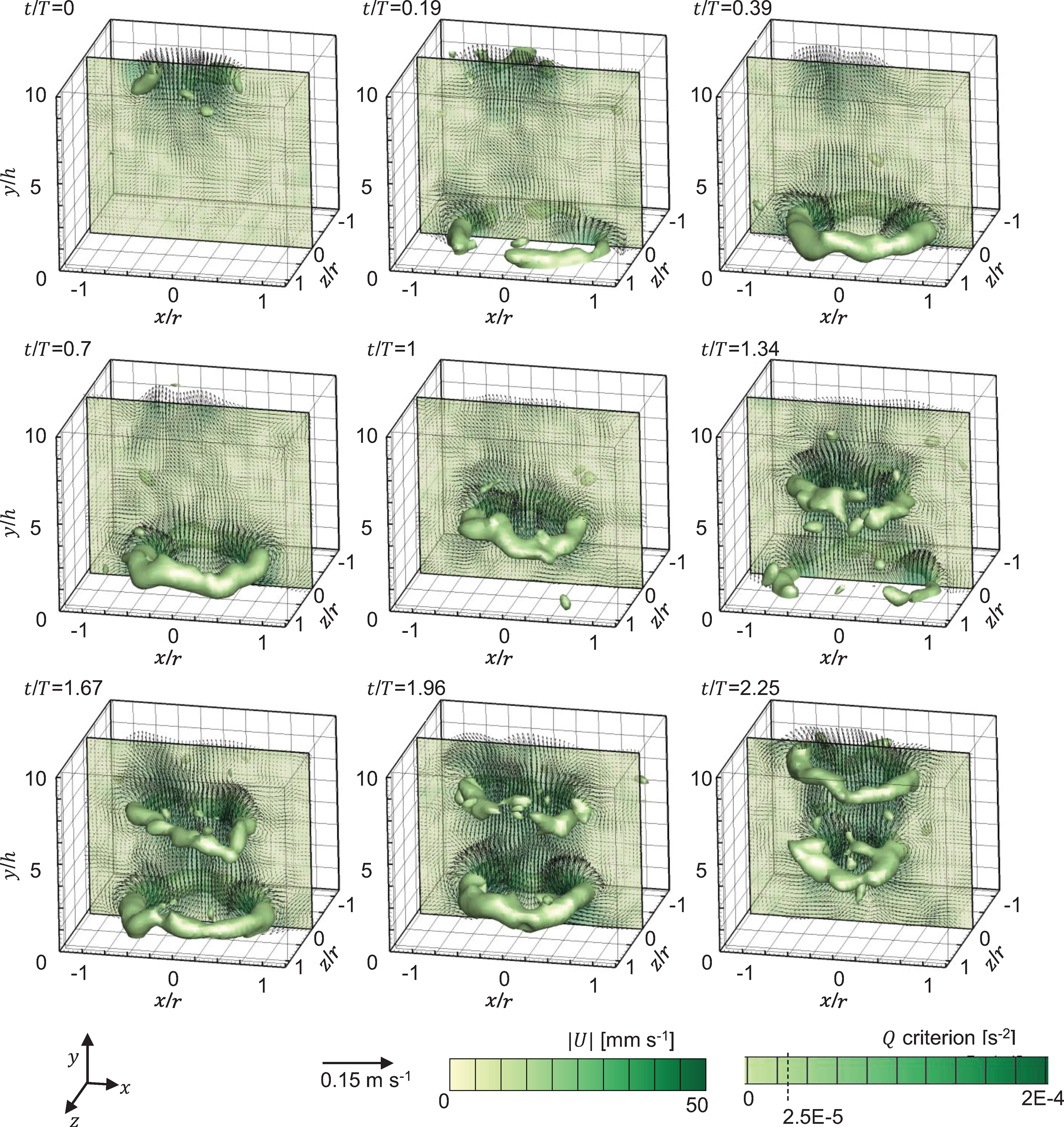
Figure 5 Flow generated by pulsations of a Cassiopea medusa with no oral arms, visualized via Q–criterion isosurfaces (at Q = 2.5×10^-5 s^-2), obtained from 3D PTV measurements. Contours are overlaid with in-plane velocity vectors at z/r = 0. Flow fields from two consecutive pulsation cycles are shown. Non-dimensional time (t/T) is defined relative to the time period (T) of the first bell pulsation cycle (=1.18 s). Time points shown for the first bell pulsation cycle (T ≈ 1.18 s) include: 0% PS (t/T = 0), 50% PS (t/T = 0.19), 100% PS (t/T = 0.39), 50% RS (t/T = 0.7) and 100% RS (t/T = 1). Time points shown for for the second bell pulsation cycle (T ≈ 1.46 s) include: 50% PS (t/T = 1.34), 100% PS (t/T = 1.67), 50% RS (t/T = 1.96) and 100% RS (t/T = 2.25). PS, power stroke (bell contraction); RS, recovery stroke (bell relaxation).

During the next bell pulsation cycle, the SVR from the previous cycle further contracted in size. A new SVR started to form near the bell at 50% PS of cycle 2 (t/T = 1.34), while the SVR from cycle 1 started to show circumferential non-uniformities in vorticity magnitude. A fully formed SVR is observed near the medusa bell at the end of PS in cycle 2 (t/T = 1.67). Circumferential breakdown of the SVR from cycle 1 is seen at 50% RS in cycle 2 (t/T = 1.96), along with upward propagation of the SVR from cycle 2. Bell expansion resulted in contracting the SVR from cycle 2 at 100% RS in cycle 2 (t/T = 2.25), while the interaction of the SVRs from both cycles augmented the circulation of the SVR from cycle 1 (as evidenced by increase in size of SVR of cycle 1).

3.2.2 Computational Results

Figure 6 shows the contours of the magnitude of vorticity for numerical simulations of a pulsing medusa with no substrate (A) and resting against the substrate (B) resting against the substrate (top, a) and without the substrate (bottom, b). Velocity vectors are taken in a 2D plane through the center of the medusa, and the arrows are proportional to the magnitude of flow. Snapshots show the beginning of the fourth stroke cycle (i) and 20%, 40%, 60%, 80%, and 100% through the stroke cycle (ii-vi). In both cases, SVRs form during the contraction (i-ii) and oppositely spinning regions of vorticity form during the RS (iii-iv), which potentially correspond to stopping vortices. The SVRs are stronger when the substrate is present (as seen by comparing the magnitude of vorticity in the vortex rings in the jets above the medusa). As a result, the upward jet is stronger when a substrate is present as these coherent vortex rings above the medusa direct the flow upwards. This can be observed by noticing the large velocity vectors (corresponding to larger flow magnitudes) within the vortex rings during the PS (i-ii) and during the resting phase after the RS (v-vi). Notice also that the vortex rings have been advected farther above the medusa for the case with the substrate (top, a).

FIGURE 6

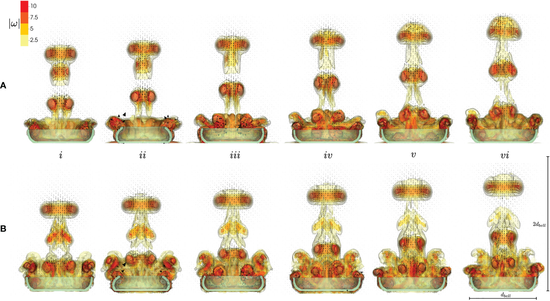
Figure 6 Velocity vectors overlaid on contours of vorticity magnitude, obtained from numerical simulations. Vorticity and velocity vectors were extracted at a 2D slice through the center of the numerical bell. Numerical simulations include a medusa resting against the substrate (A, top) and with no substrate (B, bottom). Snapshots show the beginning of the fourth stroke cycle (i) and 20%, 40%, 60%, 80%, and 100% through the stroke cycle (ii-vi).

Figure 7 shows the Q-criterion isosurfaces of flow for the numerical simulations with a substrate (a) and without a substrate (b). The contours are overlaid with velocity vectors extracted at the central plane. At the beginning of the fourth pulse (i), the three SVRs generated during the initial three stroke cycles may be observed in the wake above the medusa. During this fourth pulse cycle, the first and second SVRs merge (ii-iii) for the case with a substrate, and the second SVR dissipates in the case without a substrate. By the end of the recovery stroke (vi), the new SVR is advected into the wake above the medusa. Similar to the experiment, each SVR is readily observed as it is advected into the wake. A circumferential breakdown of the SVR’s may also be observed in the numerical model, particularly for the third SVR. Similar to the experiment, the stopping vortices are not readily apparent, but oppositely spinning vorticity is generated during the bell expansion. When comparing the substrate (a) and no substrate (b) cases, it is readily observed that the jet is weaker for the no substrate case and the SVRs are not advected as far.

FIGURE 7

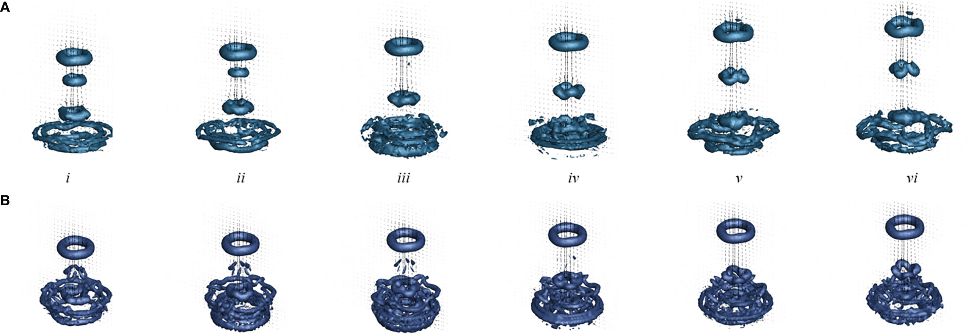
Figure 7 Q–criterion isosurface of flow generated by pulsations of a numerical Cassiopea medusa with no oral arms where the isosurface is drawn at Q = 5 s^-2. Velocity vectors were extracted at a 2D slice through the center of the numerical bell. Numerical simulations include a medusa resting against the substrate (A, top) and with no substrate (B, bottom). Snapshots show the beginning of the fourth stroke cycle (i) and 20%, 40%, 60%, 80%, and 100% through the stroke cycle (ii-v).

3.3 Velocity Distributions

3.3.1 Experimental Results

Radial distribution of 3D velocity magnitude was extracted from 3D PTV based velocity fields during cycle 1 at 3 different vertical distances from the substrate (y/h: 2.5, 5, 7.5) and at 3 cross-sectional planes differing in width (z/r: -0.5, 0,0.5), and are shown in Figure 8. At the closest vertical station (y/h = 2.5), peak jet velocity increased with increasing cycle time for all 3 width-wise (i.e. z/r) locations (compare y/h = 2.5 profiles across Figures 8A-C). Further, jet width narrowed with increasing cycle time, which is supported by the contracting cycle 1 SVR in Figure 5. With increasing vertical distance from the substrate, peak jet velocity diminished in magnitude for all width-wise locations (compare y/h = 5 profiles across Figures 8A-C). Interestingly, at the farthest vertical station, peak jet velocity was realized at the start of PS and noticeably lower than peak velocities observed with increasing cycle time (compare y/h = 7.5 profiles across Figures 8A-C). This is likely due to residual flow from the previous pulsation cycle and diminishing influence of medusa pulsations at vertical distances far from the bell. For a given vertical station (y/h), peak jet velocity was largest for the central plane (z/r = 0) as compared to the 2 non-central planes (z/r ≠ 0). Velocity distribution was not symmetric when comparing the 2 non-central planes at a given vertical station. Though bell expansion in RS generally diminished the jet velocity, unidirectional upward flow is seen throughout the pulsing cycle due to self-advection of the SVR.

FIGURE 8

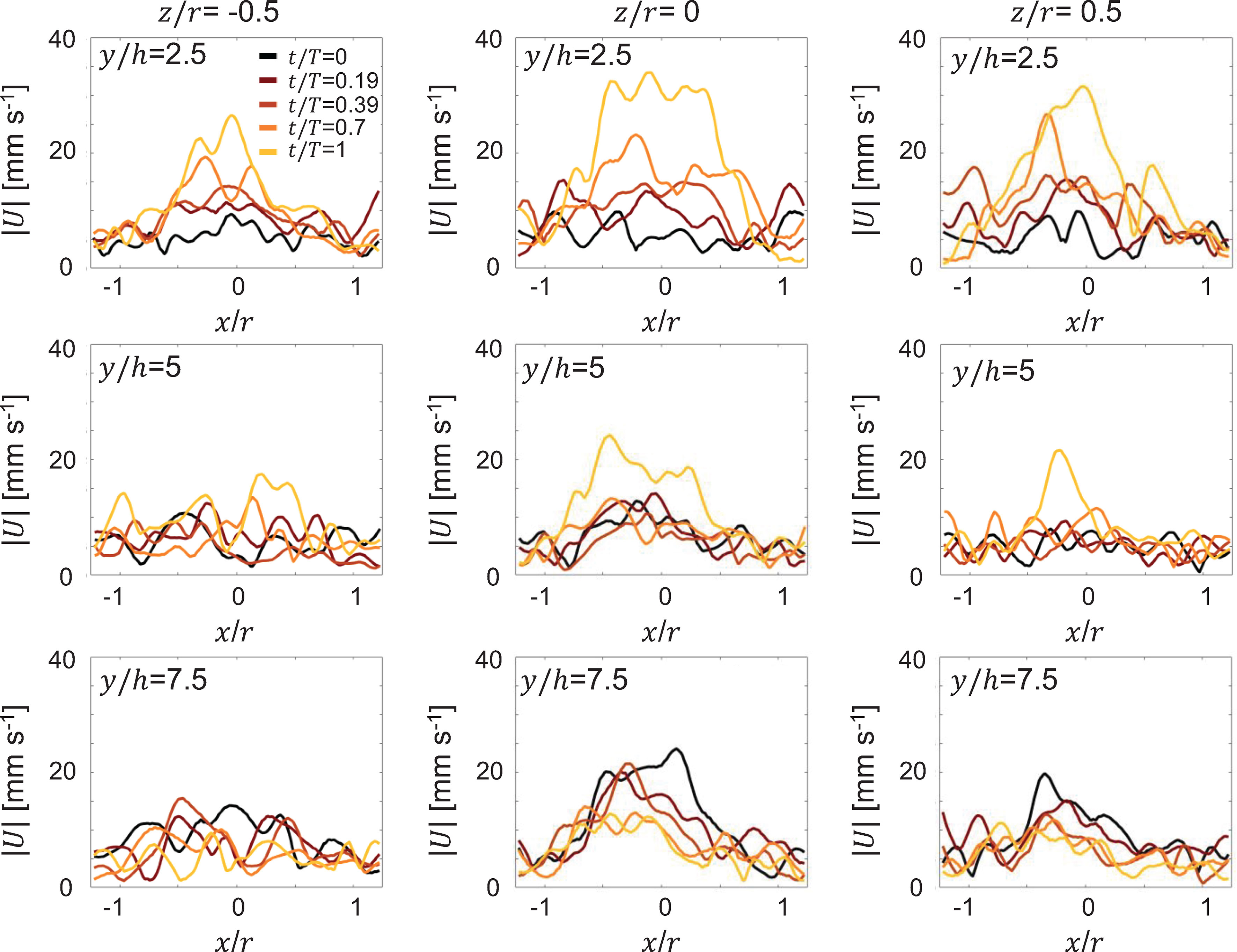
Figure 8 Radial distribution of 3D velocity magnitude (|U|) obtained from 3D PTV measurements on a Cassiopea medusa with no oral arms. Left, middle, and right columns show profiles extracted at width-wise locations z/r = -0.5, z/r = 0 and z/r = 0.5, respectively. For each z/r location, velocity profiles are shown for 3 height-wise stations y = 2.5h, y = 5h and y = 7.5h. Profiles were extracted for the first bell pulsation cycle, during the same non-dimensional times as in Figure 5.

3.3.2 Computational Results

Figures 9, 10 complement Figure 6 by providing the magnitude of velocity along horizontal lines drawn at distances of (i) 0.5d_bell, (ii) d_bell, and (iii) 1.5d_bell above the jellyfish and the vertical centerline. Each plot provides the data at the beginning of and throughout the 4th pulsation cycle at 0%, 20%, 40%, 60%, 80%, and 100% of the cycle. As suggested previously, the upward jet is stronger when the substrate is present as the peak magnitude of velocity is typically larger for the medusa resting on the substrate. Figure 9 shows that both with and without a substrate, the strongest flows occur along the centerline (x=0) and vary throughout the cycle. Furthermore, the magnitude of velocity peaks as each vortex moves over the horizontal line. This phenomenon can be observed in Figure 10 where each velocity peak corresponds to the location of a vortex ring. As the vortices are advected upwards, the peak velocities are translated to the right as time increases.

FIGURE 9

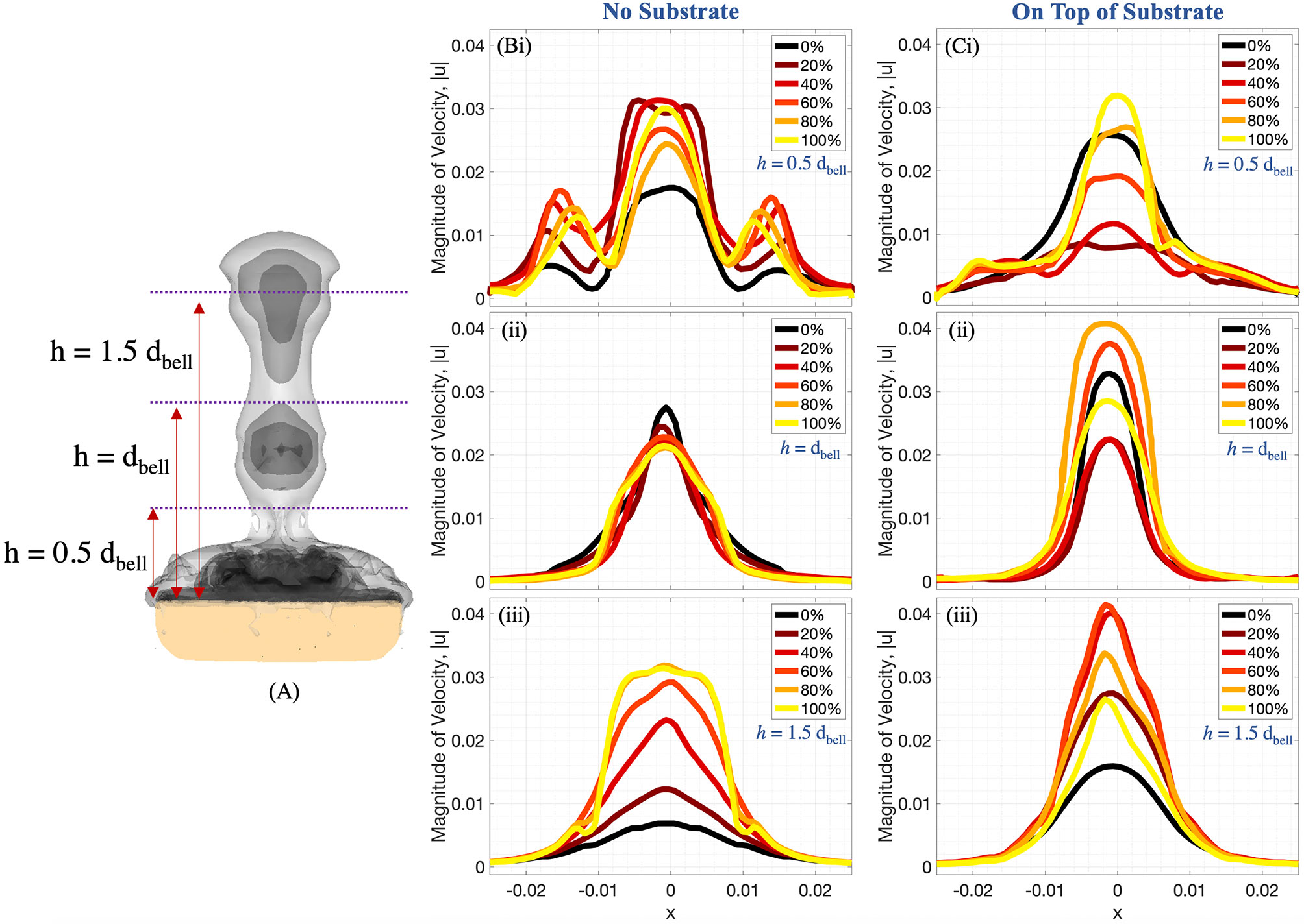
Figure 9 (A) Radial distribution of 3D velocity magnitude (in units of m s^-1) obtained from numerical simulations, computed along horizontal lines above the bell with (B) no substrate and (C) sitting on a substrate. The horizontal lines are drawn at distances of (i) 0.5d_bell, (ii) d_bell, and (iii) 1.5d_bell above the bell. Each plot provides data during the fourth pulsation cycle at 0%, 20%, 40%, 60%, 80%, and 100% of the cycle. All distances are in units of m.

FIGURE 10

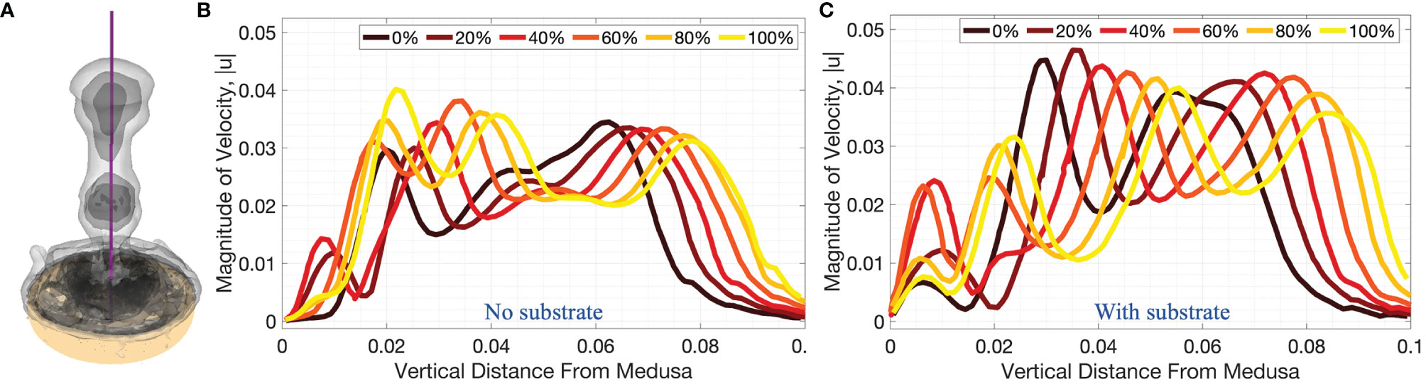
Figure 10 3D velocity magnitude (in units of m s^-1) along the vertical centerline through the middle of the numerical bell, as depicted in (A), for cases when (B) no substrate is present and (C) the bell is resting against the substrate throughout the fourth pulsation cycle (vertical distance in units of m). Centerline velocities are shown during the fourth pulsation cycle at 0%, 20%, 40%, 60%, 80%, and 100% of the cycle.

A comparison between the experiments and the numerical model may be obtained by examining the middle panel (z/r = 0) of Figure 8 and the right panel (on top of substrate) of Figure 9. When comparing the flow velocities closest to the bell (top row of Figure 8), both the experiments and numerical model show peak velocities in the range of 30-35 mm/s, with the peak value occurring at the end of the stroke cycle and near the central axis. The magnitude of the velocity drops off (roughly approaching zero) as one moves away from the central axis and beyond the bell margin. When the flow magnitude is quantified farther away from the bell (middle and bottom rows of Figure 8) the trends are less clear, with maximum flow speeds reached during the middle of the cycle. Note that these peaks in velocity magnitude occur as the vortex rings move through the vertical positions where the flows are calculated.

Figures 11, 12 show the magnitude of velocity along horizontal lines drawn at distances of (i) 0.5d_bell, (ii) d_bell, and (iii) 1.5d_bell above the bell and along the vertical centerline. Velocity magnitudes are plotted at the end of each of the four stroke cycles. It can be observed that the peak magnitude of velocity at the end of each cycle is typically larger in the case with the substrate than without. Of note is the case at the end of the 4th stroke cycle where velocities are plotted along the horizontal line at h = 1.5d_bell (see Figures 11A, Biii). In the case with the substrate (B), the initial vortex has been advected past this horizontal line, leading to a lower velocity than the case without the substrate (A). This is also illustrated in Figure 12 where the dip between the first and second peaks (moving from right to left) corresponds to a vertical distance of about 0.075 (or 1.5d_bell).

FIGURE 11

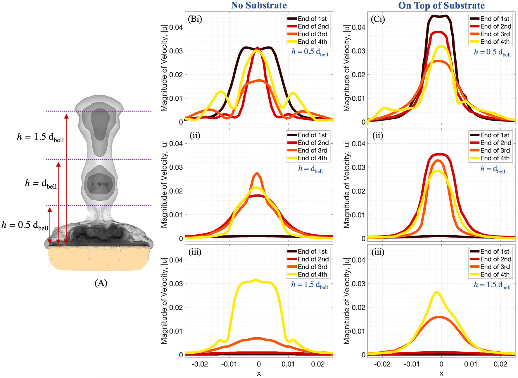
Figure 11 (A) Radial distribution of 3D velocity magnitude (in units of m s^-1) obtained from numerical simulations, computed along horizontal lines above the bell with (B) no substrate and (C) sitting on a substrate. The horizontal lines are drawn at distances of (i) 0.5d_bell, (ii) d_bell, and (iii) 1.5d_bell above the bell. Each plot provides the data at the end of the first, second, third, and fourth pulsation cycles. All distances are in units of m.

FIGURE 12

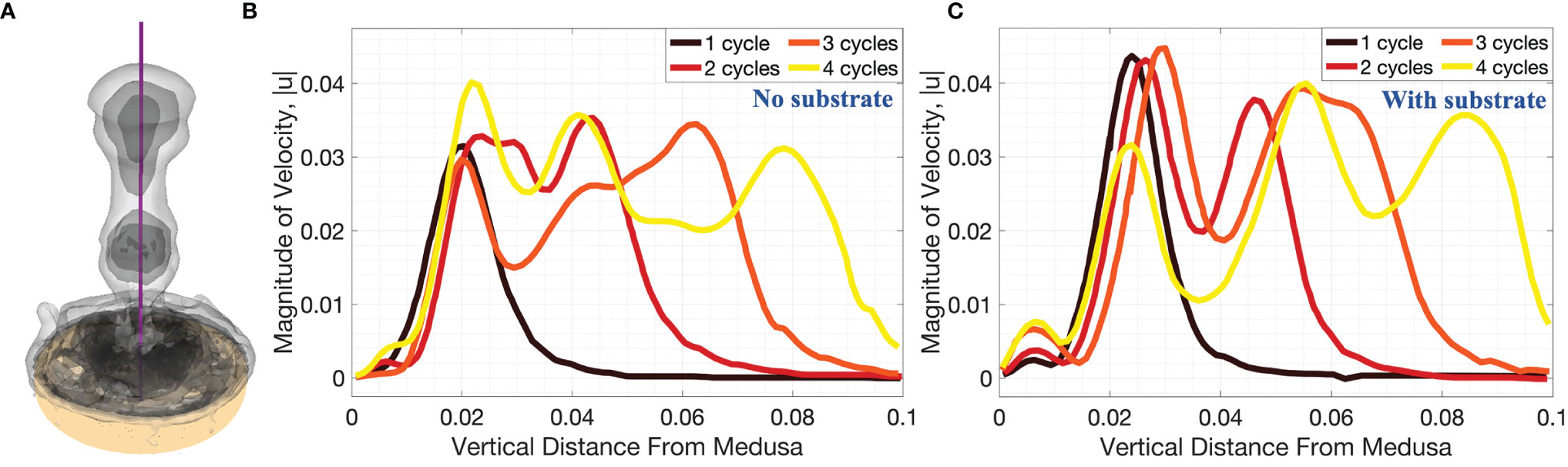
Figure 12 3D velocity magnitude (in units of m s^-1) along the vertical centerline through the middle of the numerical bell, as depicted in (A), for cases when (B) no substrate is present and (C) the bell is resting against the substrate. Data is provided at the end of the first four pulsation cycles. Vertical distance is in units of m.

3.4 Finite Time Lyapunov Exponents

Visit Visualization was used to perform forward time integration to calculate the finite-time Lyapunov exponent (FTLE) to reveal regions of repulsion. Larger values indicate separatrices in the flow that can be used to identify regions of mixing (Haller, 2000; Shadden et al., 2005; Haller, 2015). Previous analyses of jellyfish have used FTLEs to qualitatively show fluid regions where fluid is being pushed or pulled towards or away from the bell during a contraction cycle (Wilson et al., 2009). Through such analysis, fluid transport patterns of particular interest are revealed, such as those used in feeding (Peng and Dabiri, 2009; Sapsis et al., 2011) and locomotion (Franco et al., 2007; Zhang, 2008; Lipinski and Mohseni 2009; Wilson et al., 2009; Haller and Sapsis, 2011; Miles and Battista, 2019). Note that the aforementioned studies all involve actively swimming jellyfish, unlike the benthic upside-down jellyfish. However, computational studies of pulsing corals, another benthic organism, have shown similar patterns for how fluid is mixed and propelled into an upwards jet (Samson et al., 2017; Samson et al., 2019).

Our analysis was performed using a Dormind-Prince (Runge-Kutta) solver with a relative tolerance of 1e-6, absolute tolerance of 1e-7, maximum advection time of 0.625s (half a cycle), and maximum number of steps of 200. Figure 13 displays a colormap of the FTLE values for a jellyfish simulation with no substrate (A) and resting against the substrate (B). Snapshots show the beginning of the fourth stroke cycle (i) and 20%, 40%, 60%,and 80% through the stroke cycle (ii-v). The main difference in the flow patterns occurs within the bell. For the case without a substrate (top), there is a separation of the mixing regions within and above the bell that persists throughout the cycle (as seen by larger FTLE values above the bell). When a substrate is present (bottom), the mixing regions are separated within and above the bell during the expansion (iii-v). At the end of the expansion and beginning of contraction (i-ii), the fluid volume within the bell mixes with the fluid above the bell and this volume is pushed up and away from the medusa. This shows how new fluid is brought into the bell during each cycle when the substrate is present.

FIGURE 13

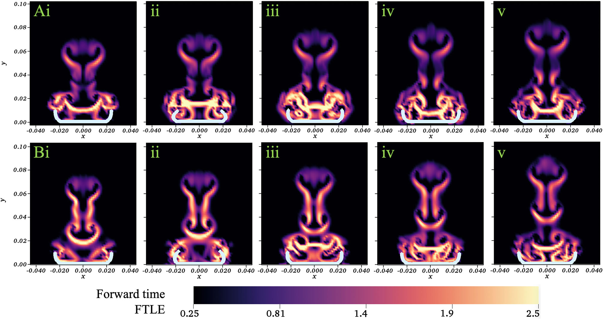
Figure 13 Colormap showing the FTLE values for a numerical simulation with no substrate (A) and resting against the substrate (B). Snapshots show the beginning of the fourth stroke cycle (i) and 20%, 40%, 60%, and 80% through the stroke cycle (ii-v). Axes scales given in units of m.

4 Discussion

In this paper, we show that the presence of a substrate enhances the vertical jet generated by pulsing upside-down jellyfish. The faster upward jet is due to the presence of stronger vortices that are formed during the pulsing cycle which serve to pull fluid toward the medusa and direct it upward into the water column. This is significant because the flow pattern brings new volumes of fluid to the medusa with each pulse for filter feeding and sampling. The strong upward jet then advects the fluid away, allowing new fluid to be sampled while also removing waste (Hamlet et al., 2011; Santhanakrishnan et al., 2012). Calculation of the finite-time Lyapunov exponent reveals that the volume of fluid within the bell is also ejected upwards during the pulse cycle, and this periodic clearance of water within the bell is more efficient when the substrate is present. Upside-down jellyfish are unique in this use of the substrate as they are the only genus of Scyphozoan jellyfish that rest against a surface. Other benthic organisms such as soft corals of the family Xeniidae rhythmically pulse their tentacles to expel fluid outwards (Kremien et al., 2013; Samson et al., 2017; Samson et al., 2019). However, the polyp’s tentacles do not rest against a substrate but are instead attached by a stem.

Rather than spending their time in open water, Cassiopea typically rest with their bells pressed against a substrate (e.g. ocean floor, rock, bottom of an aquarium, etc.). This allows them to position their oral arms filled with photosynthetic symbionts towards the sun. In other Scyphozoan jellyfish that swim, fluid is drawn towards the top of the bell and then moves around the sides of the bell and into the wake. The presence of the substrate effectively acts as a wall, and fluid must be drawn towards the jellyfish along this surface. The potential benefits or consequences of this set up are not immediately clear. Our numerical work suggests that the presence of a substrate strengthens the starting and stopping vortices, which in turn augments the strength of the vertical jet produced by the medusa.

In order to isolate the effect of the substrate and to allow for more resolved flow fields, the oral arms were removed in both the numerical and experimental medusae. Through observations in the field and the lab, we note that Cassiopea can rest with their oral arms contracted within the bell or extended over the bell margin. When the oral arms are contracted, we note that the basic flow pattern is the same (compare Figure 1 with oral arms and the numerical simulations in Figure 6): 1) a starting vortex ring is generated during contraction that is advected upwards and towards the central axis, 2) an oppositely spinning stopping vortex is generated during expansion (not shown in Figure 1 due to the placement of dye), and 3) pairs of starting and stopping vortices are advected together, pulling fluid upwards in a manner similar to what has been described for paddling oblate jellyfish (Dabiri et al., 2005). When the oral arms are extended over the bell, they do act to break up the starting and stopping vortices and enhance mixing (Santhanakrishnan et al., 2012). Consideration of this effect will be the focus of future experimental and numerical work, and this study will allow us to isolate the effect of the presence of oral arms through comparisons. We anticipate that the presence of extended oral arms will slow the jet with and without the substrate but will not change the jet-enhancement effect provided by the substrate.

This study also motivates additional work to consider the effect of scaling and duty cycle on substrate-enhancement of the vertical jet. Cassiopea must grow to a certain size before they turn upside down and rest on the substrate, but the range of Re through which they operate is large (on the order of tens to thousands). It is not clear how jet enhancement by the substrate scales as viscous effects become less significant for larger medusae. Another open question is to understand how the duty cycle or the interpulse duration affect the substrate-enhancement of the jet. It is known that flow is continually pulled towards the bell and upwards into the water column when the bell is at rest (Hamlet et al., 2011; Santhanakrishnan et al., 2012), but it is not clear how the substrate might augment the jet as the rest period is extended. Finally, we have not considered how the porosity of the substrate might alter jet enhancement. One would expect that at some point additional porosity would decrease jet enhancement since the no substrate case is essentially a substrate with infinite porosity. It is unclear, however, if the relationship is non-monotonic and if some amount of porosity might be beneficial.

Data Availability Statement

The raw data supporting the conclusions of this article will be made available by the authors, without undue reservation.

Author Contributions

NB performed analysis of the numerical data and wrote and edited the manuscript. MG designed and performed the experimental measurements, analyzed experimental data, and contributed to the writing and editing of the manuscript. CH wrote and edited the manuscript and contributed to the overall vision of the manuscript. AH designed the numerical simulations, performed simulations, analyzed data, and contributed to the writing and editing of the manuscript. LM directed the computational component of the research, performed numerical simulations and analysis, and contributed to the writing and editing of the manuscript. AS conceived the study design, directed the experimental component of the research, and contributed to the writing and editing of the manuscript. All authors contributed to the article and approved the submitted version.

Funding

Funding for AS was provided by the National Science Foundation CBET 1916061. Funding for LM was provided by the National Science Foundation: DMS-2111765 and CBET-2114309.

Conflict of Interest

The authors declare that the research was conducted in the absence of any commercial or financial relationships that could be construed as a potential conflict of interest.

Publisher’s Note

All claims expressed in this article are solely those of the authors and do not necessarily represent those of their affiliated organizations, or those of the publisher, the editors and the reviewers. Any product that may be evaluated in this article, or claim that may be made by its manufacturer, is not guaranteed or endorsed by the publisher.

Acknowledgments

We would like to thank Grace McLaughlin for her pictures of jellyfish flow visualization; Yasaman Farsiani and Nicolas George for their assistance with PTV measurements; and Boyce Griffith for his assistance with IBAMR. The authors would also like to thank open source tools from ediker.com and https://automeris.io/WebPlotDigitizer/ that expedited data and image analysis.

Supplementary Material

The Supplementary Material for this article can be found online at: https://www.frontiersin.org/articles/10.3389/fmars.2022.847061/full#supplementary-material

References

Arai M. N. (1997). A Functional Biology of Scyphozoa (New York: Chapman and Hall).

Google Scholar

Colin S. P., Costello J. H. (2002a). In Situ Swimming and Feeding Behavior of Eight Co-Occurring Hydromedusae. Mar. Ecol. Prog. Ser. 253, 305–309. doi: 10.3354/meps253305

CrossRef Full Text | Google Scholar

Colin S. P., Costello J. H. (2002b). Morphology, Swimming Performance and Propulsive Mode of Six Co-Occurring Hydromedusae. J. Exp. Biol. 205, 427–437. doi: 10.1242/jeb.205.3.427

PubMed Abstract | CrossRef Full Text | Google Scholar

Dabiri J. O., Colin S. P., Costello J. H., Gharib M. (2005). Flow Patterns Generated by Oblate Medusan Jellyfish: Field Measurements and Laboratory Analyses. J. Exp. Biol. 208, 1257–1265. doi: 10.1242/jeb.01519

PubMed Abstract | CrossRef Full Text | Google Scholar

Durieux D. M., Du Clos K. T., Lewis D. B., Gemmell B. J. (2021). Benthic Jellyfish Dominate Water Mixing in Mangrove Ecosystems. Proc. Natl. Acad. Sci. 118 (30), e2025715118. doi: 10.1073/pnas.2025715118

CrossRef Full Text | Google Scholar

Franco E., Pekarek D., Peng J., Dabiri J. O. (2007). Geometry of Unsteady Fluid Transport During Fluid–Structure Interactions. J. Fluid Mech. 589, 125–145. doi: 10.1017/S0022112007007872

CrossRef Full Text | Google Scholar

Griffith B. E. (2014). An Adaptive and Distributed-Memory Parallel Implementation of the Immersed Boundary (Ib) Method. Avalable at: https://github.com/IBAMR/IBAMR

Google Scholar

Griffith B. E., Luo X. (2017). Hybrid Finite Difference/Finite Element Immersed Boundary Method. Int. J. Numer. Methods Biomed. Eng. 33, e2888. doi: 10.1002/cnm.2888.E2888cnm.2888

CrossRef Full Text | Google Scholar

Griffith B. E., Patankar N. A. (2020). Immersed Methods for Fluid–Structure Interaction. Annu. Rev. Fluid Mech. 52, 421–448. doi: 10.1146/annurev-fluid-010719-060228

PubMed Abstract | CrossRef Full Text | Google Scholar

Haller G. (2000). Finding Finite-Time Invariant Manifolds in Two-Dimensional Velocity Fields. Chaos 10, 99–108. doi: 10.1063/1.166479

PubMed Abstract | CrossRef Full Text | Google Scholar

Haller G. (2015). Lagrangian Coherent Structures. Annu. Rev. Fluid Mech. 47 (1), 137–162. doi: 10.1146/annurev-fluid-010313-141322

CrossRef Full Text | Google Scholar

Haller G., Sapsis T. (2011). Lagrangian Coherent Structures and the Smallest Finite-Time Lyapunov Exponent. Chaos 21, 023115. doi: 10.1063/1.3579597

PubMed Abstract | CrossRef Full Text | Google Scholar

Hamlet C. H., Miller L. A. (2012). Feeding Currents of the Upside Down Jellyfish in the Presence of Background Flow. Bull. Math. Biol. 74, 2547–2569. doi: 10.1007/s11538-012-9765-6

PubMed Abstract | CrossRef Full Text | Google Scholar

Hamlet C., Miller L. A., Rodriguez T., Santhanakrishnan A. (2012). “The Fluid Dynamics of Feeding in the Upside-Down Jellyfish,” In: Childress S., Hosoi A., Schultz W., Wang J. (eds) Natural Locomotion in Fluids and on Surfaces. The IMA Volumes in Mathematics and Its Applications, vol 155(New York, NY: Springer), 35–51. doi: 10.1007/978-1-4614-3997-4_3

CrossRef Full Text | Google Scholar

Hamlet C., Santhanakrishnan A., Miller L. A. (2011). A Numerical Study of the Effects of Bell Pulsation Dynamics and Oral Arms on the Exchange Currents Generated by the Upside-Down Jellyfish Cassiopea Xamachana. J. Exp. Biol. 214, 1911–1921. doi: 10.1242/jeb.052506

PubMed Abstract | CrossRef Full Text | Google Scholar

Hedrick T. L. (2008). Software Techniques for Two- and Three-Dimensional Kinematic Measurements of Biological and Biomimetic Systems. Bioinspir. Biomim. 3, 34001. doi: 10.1088/1748-3182/3/3/034001

CrossRef Full Text | Google Scholar

Hoover A. P., Griffith B. E., Miller L. A. (2017). Quantifying Performance in the Medusan Mechanospace With an Actively Swimming Three-Dimensional Jellyfish Model. J. Fluid Mech. 813, 1112–1155. doi: 10.1017/jfm.2017.3

CrossRef Full Text | Google Scholar

Hoover A. P., Porras A. J., Miller L. A. (2019). Pump or Coast: The Role of Resonance and Passive Energy Recapture in Medusan Swimming Performance. J. Fluid Mech. 863, 1031–1061. doi: 10.1017/jfm.2018.1007

CrossRef Full Text | Google Scholar

Hoover A., Xu N., Gemmell B., Colin S., Costello J., Dabiri J., et al. (2021). Neuromechanical Wave Resonance in Jellyfish Swimming. Proc. Natl. Acad. Sci. 118, 2020025118–1–8. doi: 10.1073/pnas.2020025118

CrossRef Full Text | Google Scholar

Jantzen C., Rasheed C., El-Zibdah M., Richter C. (2010). Enhanced Pore-Water Nutrient Fluxes by the Upside-Down Jellyfish Cassiopea Sp. In a Red Sea Coral Reef. Mar. Ecol. Prog. Ser. 411, 117–125. doi: 10.3354/meps08623

CrossRef Full Text | Google Scholar

Katija K. (2015). Morphology Alters Fluid Transport and the Ability of Organisms to Mix Oceanic Waters. Int. Comp. Biol. 55 (4), 698–705. doi: 10.1093/icb/icv075

CrossRef Full Text | Google Scholar

Kim Y., Lai M. C., Peskin C. S. (2010). Numerical Simulations of Two-Dimensional Foam by the Immersed Boundary Method. J. Comput. Phys. 229, 5194–5207. doi: 10.1016/j.jcp.2010.03.035

CrossRef Full Text | Google Scholar

Kremien M., Shavit U., Mass T., Genin A. (2013). Benefit of Pulsation in Soft Corals. Proc. Natl. Acad. Sci. 110 (22), 8978–8983. doi: 10.1073/pnas.1301826110

CrossRef Full Text | Google Scholar

Lipinski D., Mohseni K. (2009). Flow Structures and Fluid Transport for the Hydromedusae Sarsia Tubulosa and Aequorea Victoria. J. Exp. Biol. 212, 2436–2447. doi: 10.1242/jeb.026740

PubMed Abstract | CrossRef Full Text | Google Scholar

Miles J. G., Battista N. A. (2019). Naut Your Everyday Jellyfish Model: Exploring How Tentacles and Oral Arms Impact Locomotion. Fluids 4 (3), 169. doi: 10.3390/fluids4030169

CrossRef Full Text | Google Scholar

Passano L. (2004). Spasm Behavior and the Diffuse Nerve-Net in Cassiopea Xamachana (Scyphozoa-Coelenterata). Hydrobiologia 530, 91–96. doi: 10.1007/s10750-004-3113-2

CrossRef Full Text | Google Scholar

Peng J., Dabiri J. O. (2009). Transport of Inertial Particles by Lagrangian Coherent Structures: Application to Predator- Prey Interaction in Jellyfish Feeding. J. Fluid Mech. 623, 75–84. doi: 10.1017/S0022112008005089

CrossRef Full Text | Google Scholar

Peskin C. S. (2002). The Immersed Boundary Method. Acta Numer. 11, 479–517. doi: 10.1017/S0962492902000077

CrossRef Full Text | Google Scholar

Rejniak K. (2012). Investigating Dynamical Deformations of Tumor Cells in Circulation: Predictions From a Theoretical Model. Front. Oncol. 2. doi: 10.3389/fonc.2012.00111

CrossRef Full Text | Google Scholar

Samson J. E., Battista N. A., Khatri S., Miller L. A. (2017). Pulsing Corals: A Story of Scale and Mixing. BIOMATH 6 (2), 1712169. doi: 10.11145/j.biomath.2017.12.169

CrossRef Full Text | Google Scholar

Samson J. E., Miller L. A., Ray D., Holzman R., Shavit U., Khatri S. (2019). A Novel Mechanism of Mixing by Pulsing Corals. J. Exp. Biol. 222 (15): jeb192518. doi: 10.1242/jeb.192518

PubMed Abstract | CrossRef Full Text | Google Scholar

Santhanakrishnan A., Dollinger M., Hamlet C. L., Colin S. P., Miller L. A. (2012). Flow Structure and Transport Characteristics of Feeding and Exchange Currents Generated by Upside-Down Cassiopea Jellyfish. J. Exp. Biol. 215, 2369–2381. doi: 10.1242/jeb.053744

PubMed Abstract | CrossRef Full Text | Google Scholar

Sapsis T., Peng J., Haller G. (2011). Instabilities on Prey Dynamics in Jellyfish Feeding. Bull. Math. Biol. 73 (8), 1841–1856. doi: 10.1007/s11538-010-9594-4

PubMed Abstract | CrossRef Full Text | Google Scholar

Schanz D., Gesemann S., Schröder A. (2016). Shake-The-Box: Lagrangian Particle Tracking at High Particle Image Densities. Exp. Fluids 57, 1–27. doi: 10.1007/s00348-016-2157-1

CrossRef Full Text | Google Scholar

Schanz D., Schröder A., Gesemann S., Michaelis D., Wieneke B. (2013). “Shake-The-Box: A Highly Efficient and Accurate Tomographic Particle Tracking Velocimetry (Tomo-Ptv) Method Using Prediction of Particle Position,” in 10th International Symposium on Particle Image Velocimetry—PIV13. 1–3 Delft, Netherlands:Delft University of Technology. Available at: http://resolver.tudelft.nl/uuid:b5eb6d27-bfb1-4c25-bc79-637df9c76694

Google Scholar

Shadden S. C., Lekien F., Marsden J. E. (2005). Definition and Properties of Lagrangian Coherent Structures From Finite-Time Lyapunov Exponents in Two-Dimensional Aperiodic Flows. Physica D 212 (3-4), 271–304. doi: 10.1016/j.physd.2005.10.007

CrossRef Full Text | Google Scholar

Thomases B., Guy R. (2019). Polymer Stress Growth in Viscoelastic Fluids in Oscillating Extensional Flows With Applications to Micro-Organism Locomotion. J. Nonnewton. Fluid Mech. 269, 47–56. doi: 10.1016/j.jnnfm.2019.06.005

CrossRef Full Text | Google Scholar

Tytell E. D., Hsu C. Y., Williams T. L., Cohen A. H., Fauci L. J. (2010). Interactions Between Internal Forces, Body Stiffness, and Fluid Environment in a Neuromechanical Model of Lamprey Swimming. Proc. Natl. Acad. Sci. 107, 19832–19837. doi: 10.1073/pnas.1011564107

CrossRef Full Text | Google Scholar

Wieneke B. (2012). Iterative Reconstruction of Volumetric Particle Distribution. Meas. Sci. Technol. 24, 024008. doi: 10.1088/0957-0233/24/2/024008

CrossRef Full Text | Google Scholar

Wilson M. M., Peng J., Dabiri J. O., Eldredge J. D. (2009). Lagrangian Coherent Structures in Low Reynolds Number Swimming. J. Phys. Condens. Matter 21 (20), 204105. doi: 10.1088/0953-8984/21/20/204105

PubMed Abstract | CrossRef Full Text | Google Scholar

Zhang Z. J. (2008). Identification of Lagrangian Coherent Structures Around Swimming Jellyfish From Experimental Time-Series Data (Senior Thesis) (California Institute of Technology), 1–30. doi: 10.7907/KK45-ZV02

CrossRef Full Text | Google Scholar