
95% of researchers rate our articles as excellent or good
Learn more about the work of our research integrity team to safeguard the quality of each article we publish.
Find out more
ORIGINAL RESEARCH article
Front. Mar. Sci. , 22 March 2022
Sec. Coastal Ocean Processes
Volume 9 - 2022 | https://doi.org/10.3389/fmars.2022.837259
This article is part of the Research Topic Consequences of Global Change in Coastal Ecosystems from a Multidisciplinary Perspective View all 10 articles
 Kathryn McMahon1*
 Kieryn Kilminster2,3
 Robert Canto4
 Chris Roelfsema4
 Mitchell Lyons4,5
 Gary A. Kendrick6
 Michelle Waycott7,8
 James Udy9
Globally marine-terrestrial interfaces are highly impacted due to a range of human pressures. Seagrass habitats exist in the shallow marine waters of this interface, have significant values and are impacted by a range of pressures. Cumulative risk analysis is widely used to identify risk from multiple threats and assist in prioritizing management actions. This study conducted a cumulative risk analysis of seagrass habitat associated with the Australian continent to support management actions. We developed a spatially explicit risk model based on a database of threats to coastal aquatic habitat in Australia, spanning 35,000 km of coastline. Risk hotspots were identified using the model and reducing the risk of nutrient and sediment pollution for seagrass habitat was assessed. Incorporating future threats greatly altered the spatial-distribution of risk. High risk from multiple current threats was identified throughout all bioregions, but high risk from climate change alone manifested in only two. Improving management of nutrient and sediment loads, a common approach to conserve seagrass habitat did reduce risk, but only in temperate regions, highlighting the danger of focusing management on a single strategy. Monitoring, management and conservation actions from a national and regional perspective can be guided by these outputs.
Spatially-explicit risk assessment is an important tool to identify and manage habitats at a range of spatial scales from local catchments to the globe (Grech et al., 2011; Halpern et al., 2015; Turschwell et al., 2021). This requires explicit knowledge of both the focal habitat and the threats, at the same spatial scale. As the spatial extent of the focal area reduces (e.g., a region to bay), a spatially explicit approach becomes more feasible as appropriate data-sets are more readily available (Grech et al., 2011). Increasing the size of the focal area (e.g., region to bioregion or nation) becomes challenging due to knowledge gaps relating to habitats and threats and mismatches in the spatial extent, temporal overlap and types of data (Specht et al., 2015). Broadscale assessments are possible through applying an explicit range of assumptions (Halpern and Fujita, 2013).
Coastal habitats provide valuable ecosystem services (Barbier et al., 2011) but are under increasing pressure, particularly as climate change manifests (Halpern et al., 2015). Marine spatial planning is an emerging discipline to address the piecemeal governance of these often multi-jurisdictional environments, a factor believed to have contributed to declining health of marine ecosystems worldwide (Foley et al., 2013). Spatially-explicit risk assessment at appropriate scales to complement policy, such as at the state or national level could significantly contribute to improved conservation of coastal habitats. For marine habitats, Halpern et al. (2015) provided a global assessment, while Grech et al. (2011) demonstrated the applicability of the approach in the Great Barrier Reef region, part of a state. We argue that evaluating risk at a national level is critical for both marine spatial planning and the allocation of national environmental management resources. It can also provide insight for the focus of management practices which are often at much smaller scales such as local government areas or states, while also placing it in the context of risk to climate change pressures which require management at a global scale. This national approach can also feed into blue-carbon policy and actions (Commonwealth of Australia, 2019) and contribute to international sustainable development goals for oceans where currently national environmental accounts are being developed to assess the extent, condition and threats to key ecosystems including seagrass to actively inform decision-making1.
Seagrasses grow around the globe in nearshore coastal habitats, are one of the most highly valued ecosystems (Barbier et al., 2011) and are sensitive to anthropogenic pressures (Waycott et al., 2009; Turschwell et al., 2021). Despite increased management, research and monitoring, in many areas they continue to decline (Dunic et al., 2021). Terrestrial activities combined with runoff threaten seagrasses, as well as physical disturbance (e.g., dredging, trawling, and accidents at sea) and climate change (e.g., increased temperature and sea level rise). Globally, urban, agricultural and industrial runoff, coastal development and dredging are considered to be the greatest threat to seagrasses (Grech et al., 2012) and recent global trajectory analysis has shown poor water quality and destructive fishing practices are the best predictors of seagrass decline (Dunic et al., 2021).
The goal of our study is to perform a spatially-explicit risk assessment of current and future threats to seagrass ecosystems across the Australian continent, incorporating states and bioregions. To achieve this, three objectives were set: (1) to create the first national seagrass map; (2) generate relevant national threat maps and assign risk from these threats; (3) perform a spatially explicit cumulative risk assessment with the map and risk layers. Adopting a national approach enables risk to seagrass habitats to be presented at a spatial scale that is beyond the experience of most stakeholders. We suggest, as Landis (2003) proposed, that operating at these broad scales for risk assessment will allow informed management and conservation decisions. Resources and effort can be focused to mitigate risk to seagrass-dominated coastal habitats and inform where further targeted studies are of most benefit.
The approach for the spatially explicit cumulative risk assessment is summarized in Figure 1 and followed the approach of Halpern et al. (2015). This involved creating a seagrass habitat map in coastal waters of Australia (Figure 2A) and identifying and developing spatially explicit risk maps of threats to seagrass (Table 1). All layers were standardized to a 10 km × 10 km grid size, the minimum size available across all layers. The cumulative risk assessment was conducted in the online open source InVEST Habitat Risk Assessment Model (Sharp et al., 2015). Validation of the outputs (individual threat layers and cumulative risk layers) was conducted by surveying 42 seagrass experts. Scenarios were tested to demonstrate how management actions could impact cumulative risk. More details on each step are provided below.
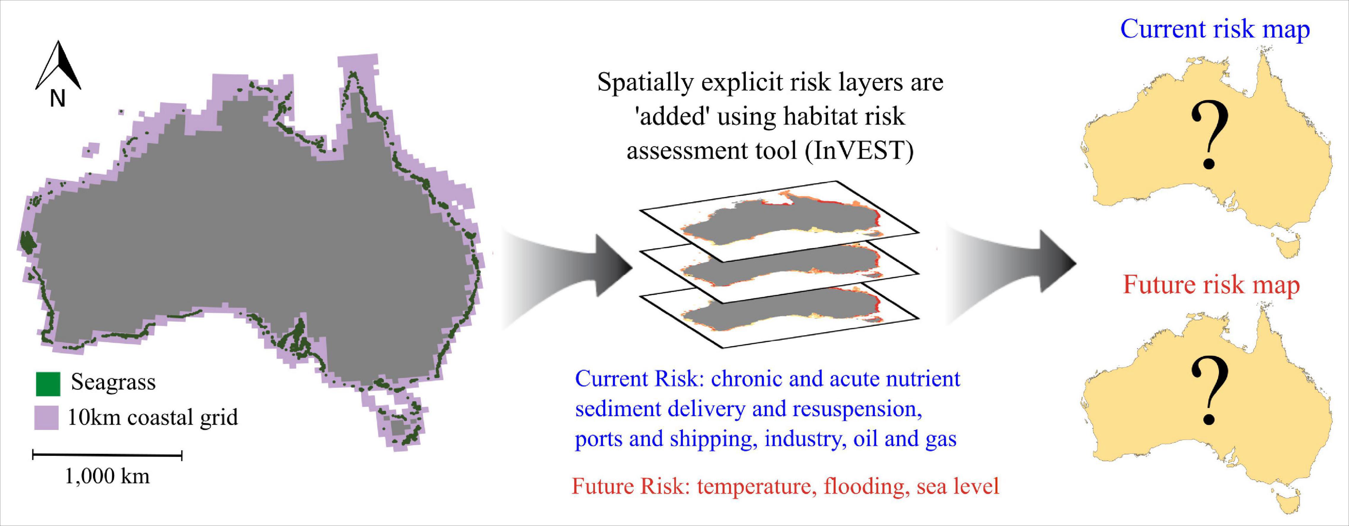
Figure 1. Flow chart to demonstrate the approach for the cumulative risk assessment in this study.
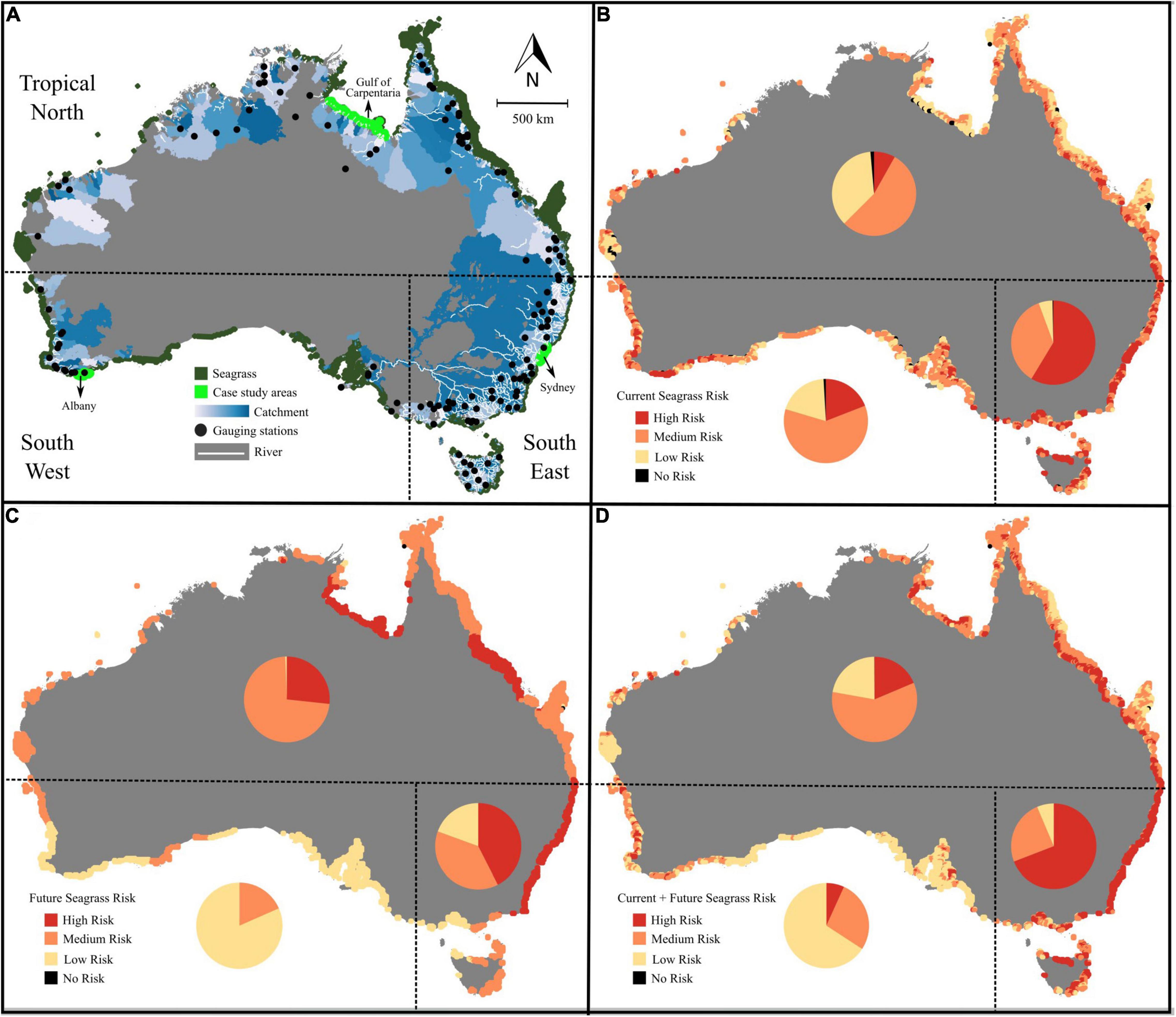
Figure 2. Australia-wide map showing three seagrass bioregions with (A) seagrass habitat, major rivers, size of catchments and case study areas of 30 pixels (as seagrass habitat generally forms a narrow band along the coast it has been expanded to make it visible at this scale), (B) cumulative current risk, (C) cumulative future risk, and (D) current and future risk combined. Pie charts in each bioregion show the proportion of cells with high, moderate or low cumulative risk. Seagrass in the south-east bioregion has higher proportion of high-risk in all scenarios.
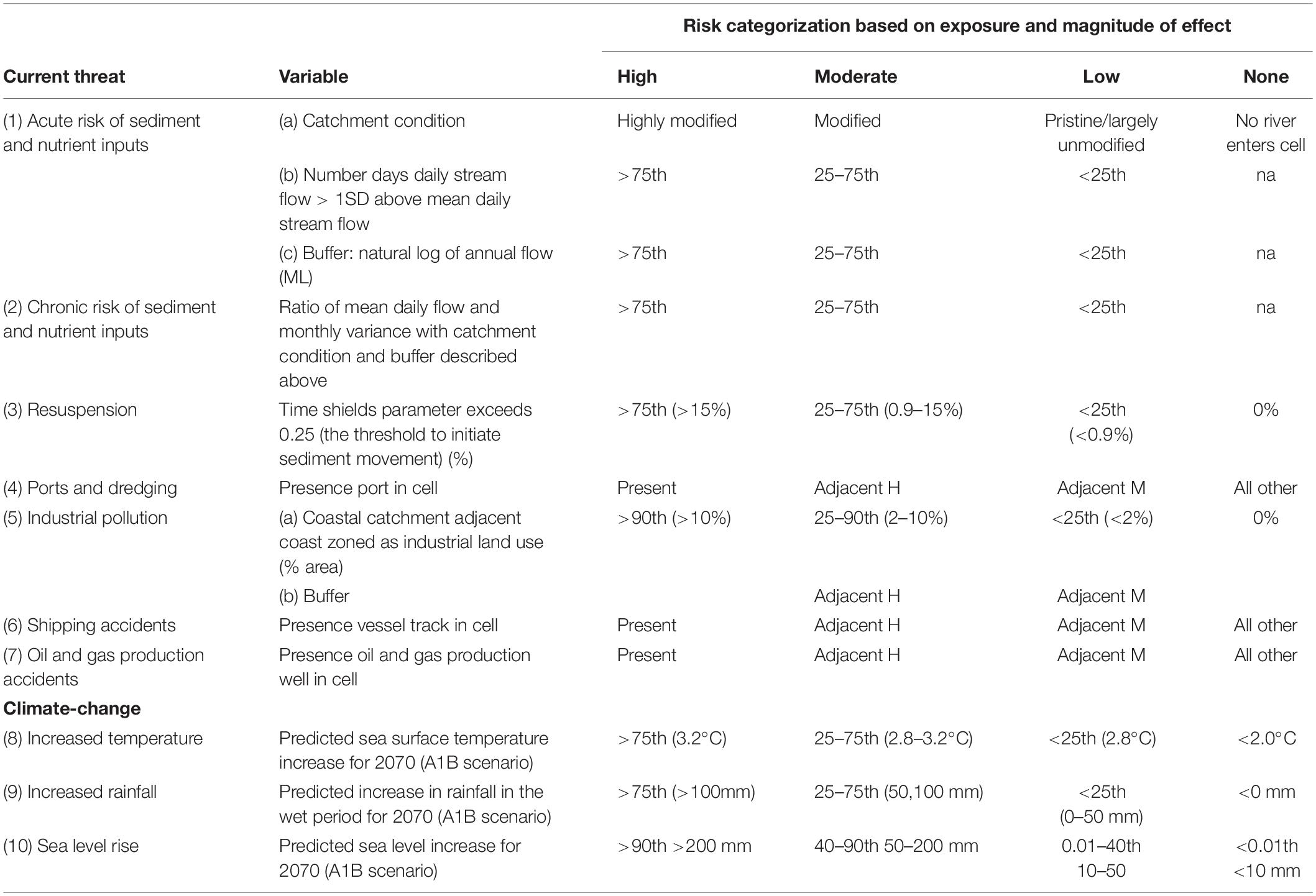
Table 1. A summary of the threats included in the cumulative risk analysis.
A nation-wide seagrass habitat map (10 km × 10 km grid size) was created based on the base-map of Mount and Bricher (2008) where each grid call was categorized as seagrass present or absent. Additional layers were added to the map: UNEP 2005 Seagrass Distribution Map (Green and Short, 2003) and an expert opinion layer from members of the Australian Centre for Ecological Analysis and Synthesis working group (Kilminster et al., 2015). The generated and freely available maps for each state are available at https://portal.tern.org.au/robert-franklin-c-canto/19365 and all have the acronym ACEAS at the end of the file name (Canto et al., 2014a, b, c, d, e, f, g). Then additional sources were added to this map (QDPI-F, 2009; McKenzie et al., 2014; TropWATER, 2016). The deep water seagrass map (QDPI-F, 2009) was categorized as the probability of seagrass occurrence. All cells with a probability of 25% or above were included. This final map is the maximum observed seagrass extent, as the data sources that generated the map span 1976–2014. Therefore, presence does not imply that seagrass is currently present, but there is the potential for seagrass to be present. In the north of Australia there was paucity of information, and even with the expert knowledge layer, we acknowledge that there may be areas of potential seagrass habitat that have not been identified. Additionally, due to the long timescale of observations, there may be areas that are no longer viable for seagrass habitat due to environmental change.
We attempted to find Australia wide, spatially explicit (10 km × 10 km grid size) datasets that represented threats to seagrass habitat identified by Grech et al. (2012) based on two categories: current anthropogenic and climate-change threats. Data was not available for all threats identified by Grech et al. (2012) at a national scale (Supplementary Table 1). Seven data layers were acquired for current anthropogenic threats representing the top four ranked threats globally (Grech et al., 2012) and three climate-change threats were acquired (Table 1). The anthropogenic threats include: (1) acute risk of sediment and nutrient inputs; (2) chronic risk of sediment and nutrient inputs; (3) resuspension; (4) ports and dredging; (5) industrial pollution; (6) shipping accidents and (7) oil and gas production accidents. The climate change threats based on predictions in 2070 include: (8) increased temperature; (9) increased rainfall and (10) sea level rise. These are available at https://catalogue.aodn.org.au/geonetwork/srv/eng/catalog.search#/metadata/0419a746-ddc1-44d2-86e7-e5c402473956?uuid=0419a746-ddc1-44d2-86e7-e5c402473956 (Canto et al., 2016). Due to the data types available at the national scale sometimes multiple inputs were required to generate each threat layer (see Table 1).
To assign the risk for each threat layer, the standard approach of Kaplan and Garrick (1981) was followed where risk is calculated based on the likelihood defined by exposure and magnitude, with the consequence defined as the vulnerability of seagrass habitat to that threat. Exposure was based on the spatial co-location of the seagrass grids and threat layers. Magnitude of the threat was based on the intensity of threat in that cell categorized into: no risk = no exposure to threat, Low, Moderate or High likelihood following the approaches of Sharp et al. (2015) (Table 1). We used two main approaches to assign a Low, Moderate and High likelihood of risk. For Port infrastructure and dredging, Shipping accidents and Oil and gas well accidents, the approach was simple, if it was present in a grid cell it was categorized High risk, cells adjacent to High were categorized Moderate, adjacent to moderate categorized as Low and all other cells were categorized as No risk. For all other threats there were quantitative values so the magnitude categories were based on these numbers. However, the quantitative relationship between the magnitude of the threat and seagrass response or condition was unknown for most threats. This uncertainty combined with the following two factors led us to incorporate a standard approach for assuming risk. Firstly, different seagrass species have different tolerances to the threats we assessed (e.g., Lee et al., 2007). Secondly, across Australia there are three bioregions with a unique suite of species (Kilminster et al., 2015) so it is likely that different species and bioregions will have different tolerances. We assumed a similar risk profile over the continental scale and based it on percentiles with grid cells <25th percentile classified as Low, 25–75th as Moderate and >75th High (Table 1). This approach was not followed in two of the threat layers, industrial pollution and future risk from sea level rise due to the nature of the data and our understanding of the potential risk. The detailed approach for each threat to define exposure and magnitude is detailed below and the risk map for each threat at the national scale is presented in the Supplementary Figures 4–13.
This threat was divided into two threat layers: acute sediment and nutrient inputs and chronic sediment and nutrient inputs, as the frequency and magnitude of delivery of nutrients and sediments from rivers into coastal environments is likely to have differential effects on seagrasses. We assumed that continual supply of nutrients or sediment over time would be a chronic risk to seagrasses primarily from smothering and eutrophication, whereas pulsed events would be an acute risk to seagrass primarily due to turbid plumes. Both forms of sediment and nutrient delivery have been demonstrated to have negative effects on seagrass (e.g., Cardoso et al., 2010; Lambert et al., 2021).
This threat layer was derived by considering the catchment condition moderated by the likelihood of large pulses of flow along river channels as well as the total volume of the flow. Specifically, the disturbance of the catchment (as identified in the National Estuary Audit 2000, n = 974 estuaries2) was used to describe catchment condition. As sediment and nutrient loads are strongly linked to catchment clearing and land use, we assumed that catchments that were near pristine and largely unmodified would pose a low risk to seagrasses in terms of sediment and nutrient loads. Similarly, the highest risk would be from catchments which are extensively modified, with a moderate risk from those moderately modified.
We considered that estuaries receiving very pulsed streamflow were more susceptible to acute nutrient and sediment loads. To determine the pulse regime, we compiled streamflow data from the Australian Bureau of Meteorology supplemented by the Western Australian Department of Water Data3, 4 () which described the daily flows from the period 1990–1999 from 241 stream gauging stations Australia-wide. Gauging stations within 250 km of the coast were ‘matched’ to the nearest point on the Australian coastline linked to the appropriate waterway, and estuaries matched with their nearest streamflow. We then calculated a pulse metric based on the number of days which daily streamflow was greater than 1SD above the mean daily streamflow [determined on ln(ML + 0.01) of daily data for each gauging station]. This is a generic threshold and the choice of 1SD was to capture the majority of the ‘above baseline’ flows. We then applied the criteria that if the pulse metric was <25th percentile, then streamflow was more constant so acute risk was assumed to be zero. If the pulse metric was within the 25–75th percentile, the acute risk was assumed to be reduced and acute risk greatest for estuaries where the pulse metric >75th percentile. The risk of acute sediment and nutrient delivery for each estuary was determined based on the catchment condition and pulse metric as summarized in Supplementary Table 2, where 4 is high risk, 3 moderate risk and 2 low with one indicating no risk. Different risk categories were assigned based on the combination of catchment condition and streamflow. For example, for acute nutrient and sediment delivery, if the catchment condition was pristine or largely unmodified and the pulse metric was <25th percentile indicating that likelihood of pulse events was low, then there was no overall risk from this threat. However, at the other end of the spectrum we assumed that if the pulse metric was >75th percentile, then the likelihood of pulse events was higher and the overall risk to seagrasses would increase as the catchment modification increased (Supplementary Table 2). Streamflow data were processed and analyzed in R (R Core Team, 2021), and the code/data used are provided as Supplementary Material (SX).
Once the risk values were generated for each estuary that had been linked to the streamflow data as described above, the spatial extent of the influence of the threat, termed buffer, was considered based on annual streamflow. Areas with higher annual streamflow would have greater sediment and nutrient risks than those which received less annual streamflow. The annual flow data was derived from the same dataset as above and the metric defined as ln(annual flow, ML). Areas receiving streamflow of 20 333 ML/yr or less, were in the lowest 25th percentile, and the spatial extent of impact was considered small. A medium extent of impact was assigned for flow between 20 333 and 181 680 ML/yr (25–75th percentiles) and >181 680 ML/yr was assigned a large extent of impact. The spatial extent was estimated based on both the risk of acute sediment and nutrient risk in the estuary (1–4 above) and the streamflow category (Supplementary Figure 1). For estuary discharge points with a low risk of acute nutrient and sediment discharge and a small streamflow there was no buffer, so only the cell adjacent to the estuary discharge point, marked by X in Supplementary Figure 1 was assigned the risk. For estuary discharge points with a moderate or high risk of sediment and nutrient discharge but a small streamflow, a buffer of 1 10 km × 10 km grid cell was added around the estuary discharge point. As the streamflow increased, we assumed the spatial extent of the area at risk would increase as demonstrated in Supplementary Figure 1. The greatest spatial extent was 5 10 km × 10 km grids from the estuary discharge point which is conservative as turbid plumes during peak flood events have been measured up to 100 km from the coast (Devlin et al., 2001). Also to take into account that the risk from sediment and nutrient delivery would decline with distance from the discharge point due to dilution of sediment and nutrients (Devlin et al., 2001) we modified the risk level of the buffer with distance from the discharge point. The way the modification occurred was dependent on both the acute nutrient and sediment delivery risk level and the volume of the flow. For low acute sediment and nutrient risk there was no change in the risk level in the buffer. For moderate and high acute sediment and nutrient risk the risk declined for all cells adjacent to the discharge point by one risk level. For example with a high acute sediment and nutrient risk, all cells in the buffer dropped to moderate. But under moderate and high sediment and nutrient risk with a high streamflow, this risk was kept for one adjacent cell, and then all other cells in the buffer declined by one risk category (Supplementary Figure 1). The risk likelihood output is displayed in Supplementary Figure 4.
The chronic sediment and nutrient input risk was derived following a similar approach as the acute risk, but the flow metric varied. We considered that water bodies which received their streamflow more constantly throughout the year were more susceptible to chronic nutrient and sediment load. To categorise the hydrologic regime, we calculated a hydrologic metric based on the ratio of the mean daily flow and the monthly variance. The rationale was to create a metric that reflected the constancy of the streamflow where lower values indicated a more constant flow over monthly time periods and higher values indicated more patchy flow. This captured a different timescale to acute sediment and nutrient threat. If the hydrologic metric was <25th percentile, then streamflow was more constant so chronic risk assumed to be greater. If hydrologic metric was >75th percentile, streamflow was more patchy, so chronic risk assumed to be reduced. No adjustment was made for estuaries where hydrologic metric was between 25 and 75th percentiles. Once again the final risk in the estuary was estimated based on the catchment condition and the hydrologic metric as summarized in Supplementary Table 2 and the buffer generated based on the annual flow as described for acute sediment and nutrient risk (Supplementary Figure 1). The key difference between the chronic and acute risk metrics is that the acute metric is cumulative across the time period (i.e., it is an absolute value of the number of days for which flow exceeded a threshold) and the chronic metric is a relative value that integrated across the time period to categorize daily streamflow in context of how variable flow is at the monthly scale. The risk likelihood output is displayed in Supplementary Figure 5.
The industrial pollution layer was generated from the industrial class cover of the Australian Bureau of Agricultural and Resource Economics and Sciences (ABARES) 2005–2006 land use map derived from an AVHRR satellite image5. This industrial pollution layer assumes that with more industrial land use in a 10 km × 10 km grid cell, the greater chance of industrial pollution reaching the marine environment, either through direct runoff, groundwater contamination or atmospheric deposition. In this approach, we only considered the grid cells that were adjacent to the coast, and not those further inland, hence the limitation is that we capture industrial pollution from direct run-off and groundwater contamination, but not from surface run-off from catchments further inland. The percentage of the terrestrial grid cell adjacent to the coast that contained industrial pollution was calculated, based on the number of pixels within each cell (total of 100). The categorisation of this threat was slightly modified compared to the other quantitative measures. If the terrestrial grid cells adjacent to the coastal grid cell contained no industrial land-use, then it was considered to have no exposure to industrial pollution. If less than the 25th percentile (2% of the grid cell was industrial) this was categorized as low likelihood (=low risk). The cut-off for the high risk was set at the 90th percentile (10% of the grid cell was industrial), not the 75th percentile, as we assumed a higher level of industrial pollution was need to create a high risk. Therefore a moderate likelihood (=medium risk) was assumed to occur between the 25 and 90th percentile (2–10%) and greater than the 90th percentile (>10%) a high likelihood (=high risk). Buffers were created adjacent to any moderate or high likelihood cells to account for transport of industrial pollution in the marine environment. Any marine grid cell adjacent to a high risk cell was considered a moderate risk, and those adjacent to a moderate risk cell were considered a low risk. If any grid cell was allocated more than one risk category, then the highest category was maintained. The risk likelihood output is displayed in Supplementary Figure 8.
Sediment resuspension is related to acute and chronic sediment delivery, but it represents a different pressure to seagrass ecosystems. The risk from resuspension of sediments to seagrass ecosystems is not just due to the delivery of sediment, but the sediment grain size distribution and how this interacts with waves and currents where finer sediments and greater tidal and wave energy would result in higher resuspension. The Geological and Oceanograhic Model of Australia’s Continental Shelf (GEOMACS) was used and the dataset “Percentage of the time that the Shields parameter exceeded 0.25 applied to predict the risk from resuspension. The Shields parameter defines the bed shear stress required to initiate sediment movement. When it is >0.25, conditions on the seabed are highly mobile, hence there is more chance of resuspending sediments which can have a negative impact on seagrasses due to reductions in light.
We assumed that with a greater percentage of time above the Shields parameter of 0.25 there would be a greater risk due to sediment resuspension. No quantitative relationship is known for the percentage of the time the shields parameter is above 0.25 and seagrass condition so the approach of assigning a low risk below the 25th percentile (0.8% of the time), a high risk above the 75th percentile (15.8% of the time) and a moderate risk between the two. There was no exposure and hence no risk to seagrass habitat from resuspension when the Shields parameter did not exceeded 0.25 at any time (Hemer, 2006; Hughes et al., 2010; Harris and Hughes, 2012). The risk likelihood output is displayed in Supplementary Figure 6.
The threat to seagrass habitat from port infrastructure and dredging was assessed based on the locations of ports in Australia provided by the Australian Customs & Border Protection Service6. We assumed that there was a high risk to seagrass habitat when there was a port located in a grid cell, a moderate risk in cells adjacent to a high cell, and a low risk in cells adjacent to moderate. We considered that there was no exposure to the threat of port infrastructure and development and hence no risk in all other grid cells. The risk likelihood output is displayed in Supplementary Figure 7.
The threat to seagrass habitat from shipping accidents was predicted from vessel track history in Australia sourced from the Australian Maritime Safety Authority7 over the whole 2012 period recorded with a 3 h frequency. We assumed that there was a high risk to seagrass habitat when there was a history of vessels tracking through a grid cell, a moderate risk in cells adjacent to a high cell, and a low risk in cells adjacent to moderate adjacent cells. We considered that there was no exposure to the threat of shipping accidents and hence no risk in all other grid cells. The risk likelihood output is displayed in Supplementary Figure 9.
The threat to seagrass habitat from oil and gas accidents was predicted from the location of oil and gas wells in the coastal environment. Gas pipelines were not considered, as this information is restricted. The location of oil and gas production wells was sourced from GeoSciences Australia8. We assumed that there was a high risk to seagrass habitat when an oil and gas well was in a grid cell, a moderate risk in cells adjacent to a high cell, and a low risk in cells adjacent to moderate adjacent cells. We assued that there was no exposure and hence no risk in all other grid cells. The risk likelihood output is displayed in Supplementary Figure 10.
Different seagrass species have different temperature tolerances (Lee et al., 2007) and in Australia species are distributed across locations that have a broad temperature range (Kilminster et al., 2015). Therefore some locations, such as at the range edge may be more susceptible than other locations (Jordà et al., 2012). To employ a consistent and justifiable assumption for impacts of increased temperature we used published data on short-term responses to increased temperature. This may be an overestimate of the response, as we have no understanding about adaptive capacity to changing temperatures. The majority of studies on the effects of short-term temperature increases to seagrasses have shown negative effects with increases of 2°C or more (Seddon et al., 2000; Waycott et al., 2007; Collier et al., 2011; Moore et al., 2013; Thomson et al., 2015). The OzClim Mk3.5 model 2070 predictions of sea surface temperature were used9 and the risk assigned using a percentile approach as follow, High > 3.2°C (75th percentile), Moderate 2.8–3.2°C (25th – 75th) and Low < 2.8°C (25th percentile). The predicted temperature always increased by more than 2°C so a no risk category was not assigned. The risk likelihood output is displayed in Supplementary Figure 11.
We assumed that a greater rainfall would lead to more sediment and nutrient delivery, more flooding and more low light events that could impact seagrasses (Collier et al., 2012) and hence either more acute or chronic sediment and nutrient risk to seagrasses. The predicted change in rainfall in 2070 dataset by OzClim GFDL-CM2.1 model (see Text Footnote 9) was used and we focused on the period of the year that was considered the wet period, as the OzClim predictions provided predictions based on wet and dry periods. For this threat the standard percentile risk approach was applied. We classified this data as no risk if the rainfall was not predicted to increase, low risk if it increased up to 50 mm per year (<25th percentile), moderate if it increased 50–100 mm and a high risk if it increased more than 100 mm (>75th percentile). The risk likelihood output is displayed in Supplementary Figure 12.
An increase in sea level can have a negative effect on seagrasses if the shoreline is hardened and they cannot colonize new habitats, also seagrasses can be lost on the deeper edge if light becomes limiting to growth (Waycott et al., 2007; Saunders et al., 2013). Saunders et al. (2013) modeled the impact of sea level rise on a large embayment in Queensland and found that the area of seagrass declined by 17% with a 1.1 m rise in sea level. Obviously these predictions are location specific but we used these as a guide to categorize the likelihood of the risk. Dataset on the projected departure from global mean (A1B scenario) at 2070 (mm) from 17 model simulations was used10 to quantify sea level increase. For this threat the standard percentile approach was not used as it did not align well with the predictions of seagrass loss with a 1.1 m rise as a 1 m increase in sea level was equivalent to the 75th percentile and we considered a 17% loss moderate. Therefore the percentile values used were 40th percentile (0.5 m rise) for the low – moderate cutoff, 90th percentile (2.0 m rise) for the moderate to high cutoff. If no increases were predicted, then no risk was assumed, less than 50 mm was low, 50–200 was moderate as this spanned the level predicted by Saunders et al. (2013) to have an impact, and >200 mm a high likelihood. The risk likelihood output is displayed in Supplementary Figure 13.
The consequence of the threat was based on the vulnerability rating of Grech et al. (2012) and Halpern et al. (2015), incorporating the frequency, functional impact, ability to resist, ability to recover and certainty of the impact of that threat (Table 2). Similar but not identical threats were assessed in these studies so to develop the consequence ratings, the threats in each study were grouped into similar categories, the consequence rating ranked, and then the consequence measure grouped into high, moderate and low consequence (Table 2).
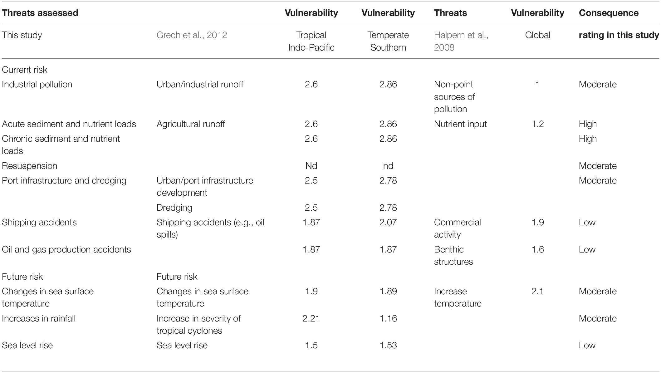
Table 2. A comparison of the vulnerability measure for each threat addressed in this study in comparison to other studies that have assessed the vulnerability of threats to seagrass habitat.
The cumulative risk assessment was conducted in the online open source InVEST Habitat Risk Assessment Model (Sharp et al., 2015). The final seagrass map was overlayed with the likelihood of each threat layer defined as either 1- no exposure, 2- low, 3- moderate and 4- high likelihood. The consequence layer in Invest was kept the same as the likelihood layer but the consequence of the threat was simulated by replicating the layer. If the consequence was low, one layer was used, moderate, two replicate layers and high, three replicate layers. In InVEST the cumulative risk (R) of multiple threats layers (J) is calculated based on the euclidean distance as
The euclidean distance provides a conservative, additive approach due to the uncertainty of the response to interactions between threats (Halpern and Fujita, 2013). The cumulative risk output was scaled into four categories, No cumulative risk, <25th percentile low cumulative risk, 25–75th percentile moderate risk and >75th percentile high cumulative risk.
A cumulative risk assessment was conducted for three sets: (1) current threats only (n = 7), (2) climate change threats based on 2,070 predictions (n = 3) and (3) combining current and climate change threats that simulate 2070 scenarios. When combining the current and climate change sets, no changes were made to the current risk assessment, we assumed no changes on the threat and no changes in the vulnerability due to adaptation occurred. Therefore this provides a tool to identify hotspots of risk under current conditions and into the future, helping to prioritize management actions. To demonstrate how risk varies spatially and under these cumulative risk calculations the data was summarized by each bioregion, the South West, South East and Tropical North (Figure 2). In addition, an area within bioregion containing 30 10 km × 10 km grid cells was selected to demonstrate in a higher resolution the spatial variability in current and future threats and cumulative risk.
The outputs from the nation-wide risk assessment for each threat layer (n = 10) and for the cumulative risk layers from two sets, current and climate change based on 2,070, were assessed by 42 seagrass experts at the Australian Marine Science Association Conference in 2015 (Supplementary Figure 2). These experts self-selected and had experience working in seagrass research or management from particular regions in Australia and only provided validation data from the areas they had experience in. Two approaches were used: a quantitative assessment to assess how the risk assignment for each threat based on exposure, magnitude and consequence of the threat and the cumulative risk assessment model output deviated from the expert opinion; and a qualitative assessment to measure the confidence of the experts in the same outputs. For each approach, the experts were asked to assess three areas in their region of expertise (Supplementary Table 3). The qualitative assessment was carried out first on one grid cell in a particular region, then the experts were shown the model outputs and asked to give a confidence rating across all cells in that region, following the methods of Hoque et al. (2018). For the quantitative assessment experts were asked to provide their opinion of whether it was 0 = no risk, 1 = low risk, 2 = moderate risk and 3 = high risk for each threat input layer and cumulative risk assessment output layer. For the qualitative assessment experts were asked to provide a ranking of 0 = no confidence, 1 = low, 2 = moderate and 3 = high confidence in the information provided.
To test how nutrient and sediment management strategies impact the overall cumulative risk under current conditions the risk rating for chronic and acute sediment and nutrient risk were modified and cumulative risk model re-run. Cells with high or moderate risk from nutrient and sediment load were dropped down one risk level, but cells already with low risk remained at low. This data was summarized by bioregion.
Individual threat layers showed different spatial patterns of risk as demonstrated by the examples from Tasmania (Figure 3) and compared to the cumulative risk results (Figure 2), reinforcing the value of assessing multiple threats cumulatively (Supplementary Figures 4–9). For example, the Tropical North case-study (Gulf of Carpentaria) has very low current risk levels and the South East case-study (Sydney) has much higher current risk levels, yet similar future cumulative risk categories were derived for both of these regions (Figure 4). In the Tropical North case-study the high cumulative risk from future climate change threats was driven by the combination of high risk from increased temperature and sea-level rise, whereas in the South East case-study it was driven by the combination of high risk from temperature and increased rainfall (Figure 4). This again highlights the need to consider a range of threats for management decision-making and recognizing different regions may require different strategies.
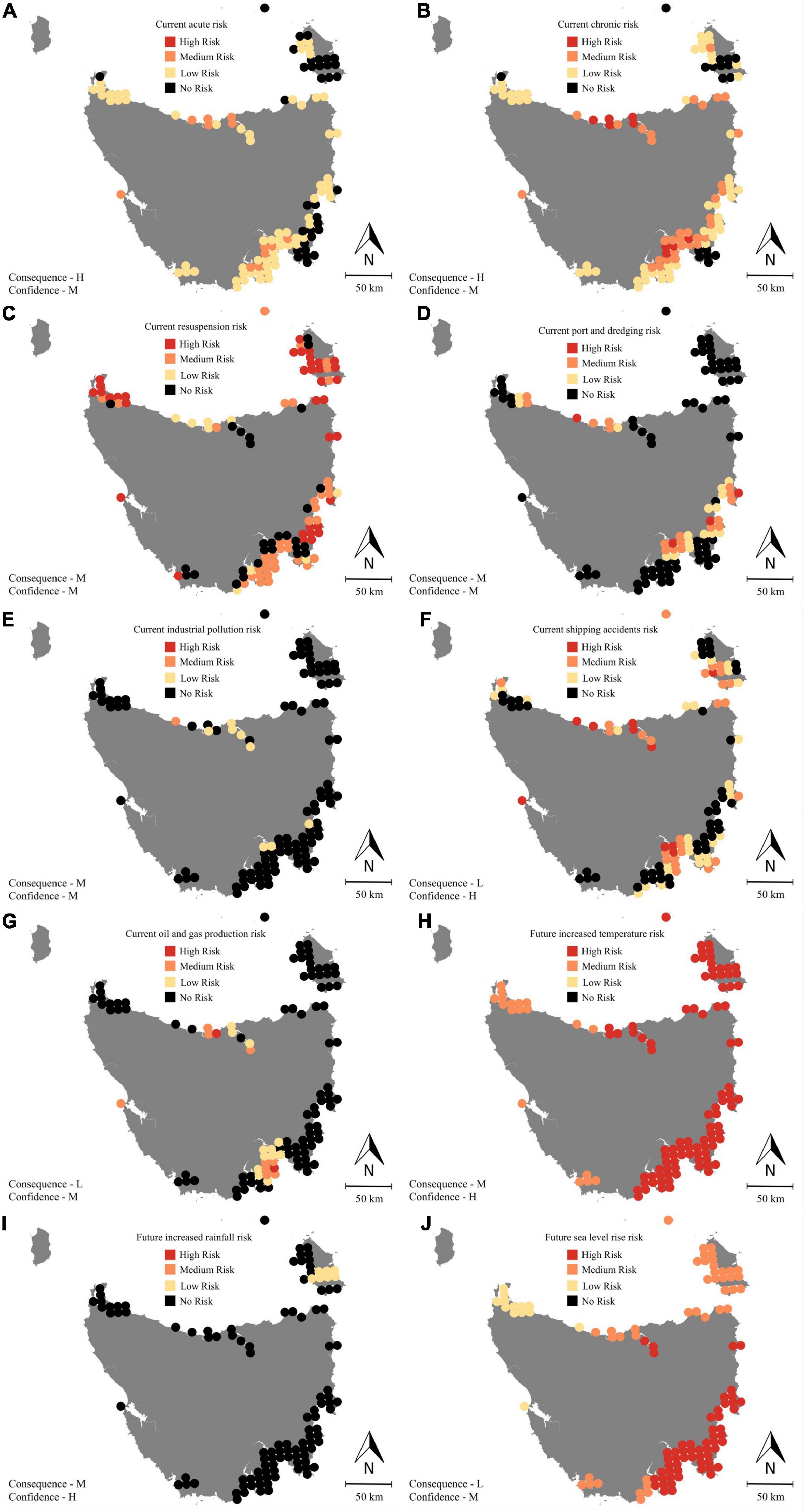
Figure 3. An example of how spatially explicit current (A–G) and future (H–J) threats were applied to Tasmania (10 km × 10 km grid cells). Only cells where seagrass is present are shown. The risk of each threat was categorized as high, medium, low or no risk if there was no exposure to that threat. Each threat was weighted based on the consequence of exposure to this threat and the confidence in the threat was assessed through a survey with experts.
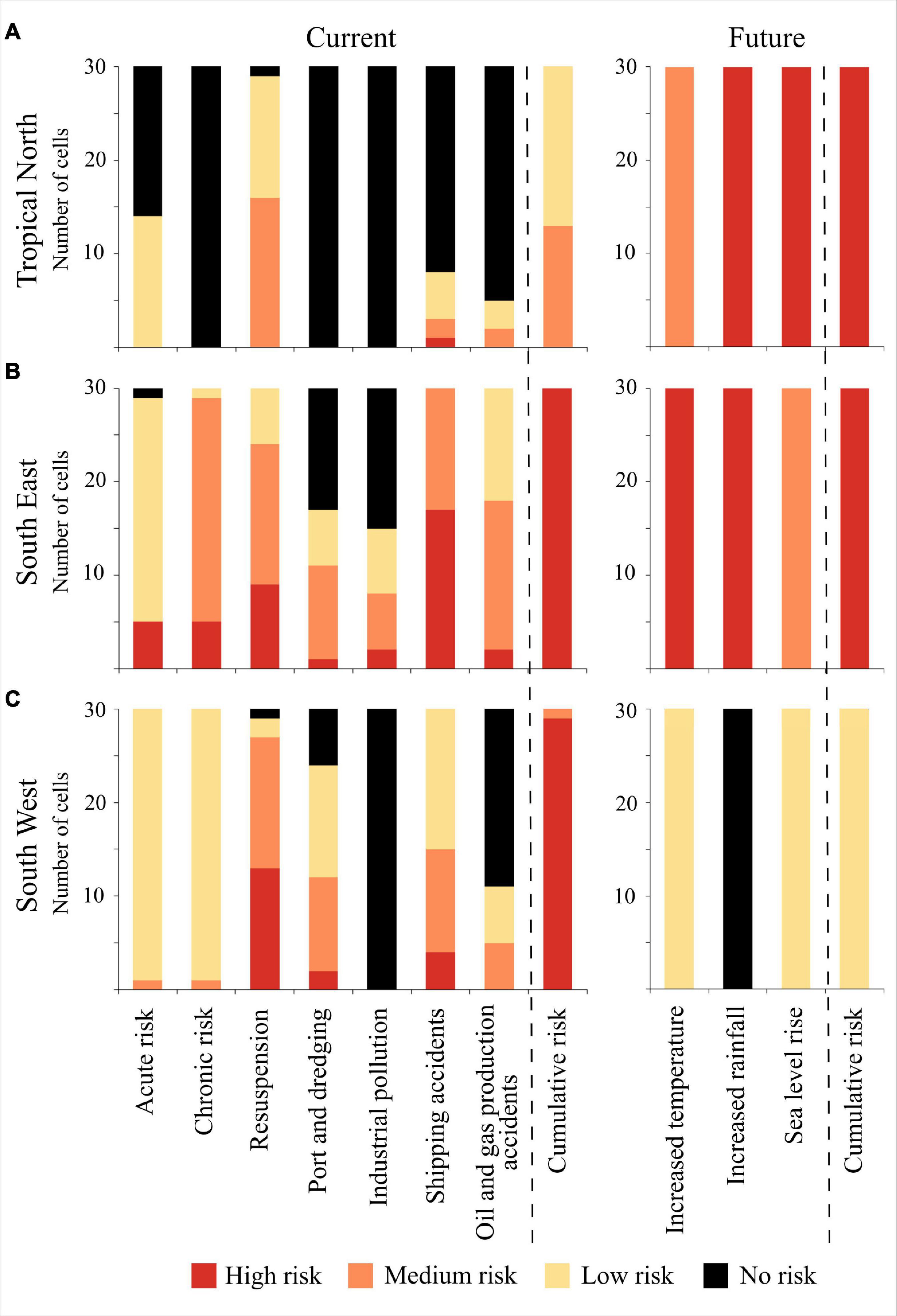
Figure 4. Case study of 30 seagrass cells from each bioregion. (A) Tropical North (Gulf of Carpentaria), (B) South East (Sydney-Newcastle), and (C) South West (Albany) showing the breakdown of individual threats contributing to the current cumulative risk (left) and future cumulative risk (right). A similar cumulative risk (e.g., high) can be derived from different combinations of individual threats.
There was much more spatial variation in the cumulative risk of current threats compared to future climate change threats, which were generally consistent across bioregional scales, the scale at which climate operates (Figure 2). When combining current and future pressures, some high risk hotspots and low risk ‘cold-spots’ changed. For example cumulative risk from current threats was lowest in the Tropical North (greatest proportion of low risk, Figure 2B), with a cold-spot in the Gulf of Carpentaria. However, when adding the high threat future pressures, this area became moderate to high risk. On the other hand, isolated hotspots of high risk that were distributed along the eastern coast of Australia under current pressures expanded into a widespread band of high risk when combined with future pressures, especially in the South East bioregion and the Great Barrier Reef World Heritage Area (GBRWHA, east coast of Australia in the Tropical North bioregion).
When simulating nutrient and sediment management strategies by reducing the areas with high or moderate risk for chronic and acute sediment risk by one category, cumulative risk in the South East bioregion reduced (Table 3). In other bioregions this did not result in the cumulative risk to seagrass habitat being reduced.
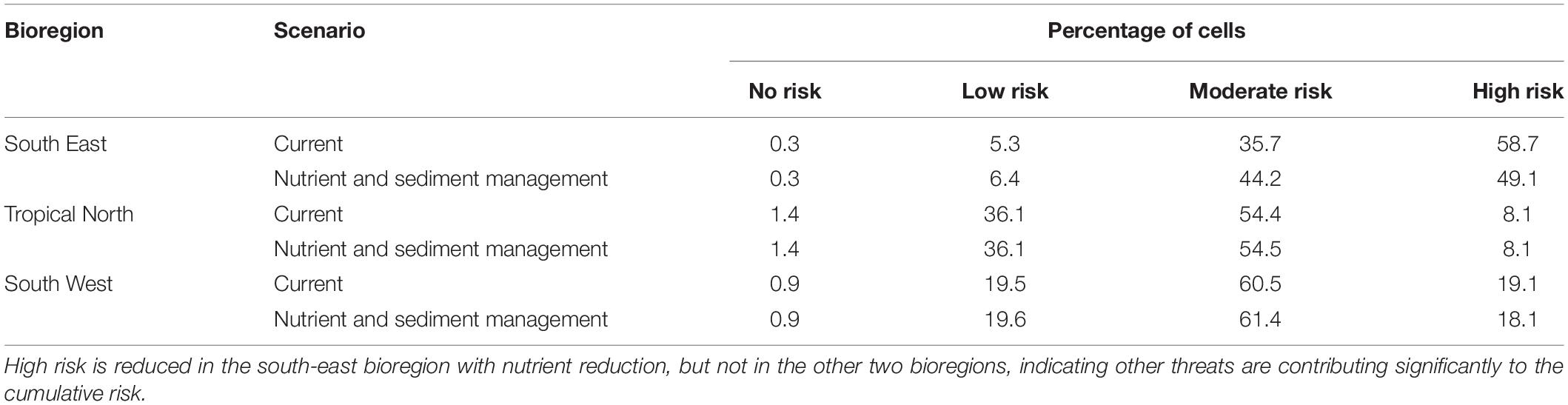
Table 3. Comparison of how the percentage of cells under the different current cumulative risk categories changes following a simulated nutrient reduction.
We generated ten spatially explicit threat layers specific for seagrass habitat across the Australian continent using a range of data sources (Table 1). When summarized across all of Australia, experts had the highest confidence in the risk assigned to climate change threats (increased temperature and changes in rainfall) as well as localized shipping accidents. There was a moderate confidence for all other layers (Supplementary Figure 3). For the quantitative assessment the experts matched quite closely the model predictions for all climate change threats as well as the risk from resuspension and shipping. For the remaining threats there was a slight overestimate of the model for threats from oil and gas wells, industry and ports and dredging, on average 0.5–0.8 units, with an overestimate of ∼1 category (1.2 units) for threat from sediment and nutrients (Supplementary Figure 3). This overestimate was mostly driven by respondents that were experts from Western Australia and Queensland indicating that their perceived threats are higher than model predictions. This is likely because most evidence for seagrass decline historically is due to eutrophication.
One of the challenges for environmental management is having information at the appropriate spatial and temporal resolution and extent to aid decision making (Specht et al., 2015). This is very apparent at national levels and across bioregions because information is disparate and is derived from local stakeholders with different types of information. We have begun to address some of the challenges by developing a set of publicly available, national, spatial threat maps representing ten pressures for seagrass ecosystems along the 35,000 km coastline of the Australian continent. It is a data resource that can be used for future work, adapted to assess other habitats or also be used as a local-scale or nation-wide tool to aid decision making in the face of multiple threats and limited resources (Pressey et al., 2007). In addition, the approach can be applied to other regions around the globe to assess risk to seagrass habitats.
This resource was then used for a spatially explicit cumulative risk analysis based on the ten threat layers, identifying hotspots of high and low risk for coastal seagrass habitat based on the exposure and vulnerability to a range of relevant pressures. This standardized approach provides a tool to enable informed decision making at a national level (Tulloch et al., 2015). Currently the Australian Federal government is developing national environmental accounts for blue-carbon habitats including seagrasses. To do this habitat maps, condition of the habitat and potential threats to these habitats is required and these are assessed over time (see Text Footnote 1). This resource can be used to support these activities. Although, many of the major identified threats to seagrass habitat were sourced (Grech et al., 2012; Turschwell et al., 2021), information at the national scale for some key threats are still missing such as trawling or aquaculture (Turschwell et al., 2021). There is still effort needed to improve the representation of threats at a national level and this aligns with the priority to address the challenges for improving ocean health, where Claudet et al. (2020) indicated more integration of information is needed to support decision-making.
High cumulative risk areas were identified based on exposure to threats from current practices. These were generally associated with population, agricultural and/or industrial centers and were distributed around Australia, although the greatest proportion was in the most densely populated South East bioregion (Figure 2B). Globally loss of seagrass habitat has been attributed to deterioration of water quality from increased nutrient and sediment loads (Waycott et al., 2009; Turschwell et al., 2021) so load reduction is a management strategy commonly used to protect seagrass habitat, although not always successful due to the complex nature of the systems (Unsworth et al., 2015). It is a current management focus in all bioregions in Australia (Jackson et al., 2016; Brodie et al., 2017). Interestingly, the high cumulative risk predicted in this study could be reduced somewhat through simulating reductions in nutrient and sediment loads, but only in the South East. In the Tropical North, around the Great Barrier Reef World Heritage Area, reducing nutrients and sediments, did not reduce the cumulative risk from current threats. The environmental protection policy for seagrass habitat in the GBRWHA, part of the Tropical North, focuses on improving water quality and managing the impacts of dredging (Anon., 2015). Grech et al. (2011) also recommended focusing management on agricultural inputs (nutrient and sediments) due to the large catchment areas. However, our analysis indicates that focusing on this alone will not reduce the risk of impact to seagrass habitat. Threats with the greatest individual risks for the Great Barrier Reef example based on our analysis, includes resuspension, ports and shipping as well as risk from increased rainfall (Supplementary Figures 6, 7, 9, 12). So reducing sediment loads may contribute somewhat to resuspension risk by reducing the pool of sediments that could be resuspended. But increased risk from rainfall requires global action to reduce the rate of greenhouse gas emissions and the changes in weather patterns. To manage for this scenario actions to increase resilience of seagrass habitats to these cumulative threats combined with interventions to facilitate recovery and or restore habitats is needed.
This study highlighted that when managing habitat based on risk at a national level; taking into account future risk from climate change altered the spatial pattern of risk. The 2,070 model projections used can be considered conservative as climate change effects may manifest at a faster rate than these predictions (IPCC, 2019). Similar to current threats, other climate change threats have also not been included such as heat waves, so further effort is needed to create these threat layers and develop a process to assign risk. Despite this, the incorporation of climate change risk into the future was valuable as it provided further insights to inform management decisions. For example, if high risk to seagrass habitat is predicted mostly from a set of current threats, reducing these specific threats could be the focus for management. But if high risk is predicted mostly from climate change threats then management actions for resilience building, facilitated recovery and restoration would be important to consider. When both current and future threats generate high risk an approach combining both sets of actions is needed. By assessing the cumulative risk from both current practices and future threats, the footprint of high risk increased, particularly in the South East and Tropical North bioregion. For example, in the globally significant GBRWHA, high risk has been identified from current threats in six hot-spots (Figure 2B) but when this is combined with threats from climate change (Figure 2C), this expands into a much larger, almost continuous band in the central and southern GBRWHA. Our approach re-affirms the importance of managing risk as a cumulative challenge (Grech et al., 2016) and the value of projecting future scenarios to guide where resilience building and restoration actions are most needed.
Cumulative risk assessment does not imply impact or predict response in a habitat. It is used as a tool to identify where multiple threats occur and assists decision-making based on a number of assumptions: that risk of multiple threats is additive; and the vulnerability of the seagrass habitats to these threats is known (Halpern and Fujita, 2013). We know that this is a simplification of the real world as the suite of seagrass species changes across bioregions and different species vary in their life-history strategy influencing their ability to resist and recover from disturbance, hence influencing their vulnerability (Kilminster et al., 2015). This has been highlighted recently where life-history was a strong predictor of the trajectory of seagrass change over time (Turschwell et al., 2021). Assemblage-specific vulnerabilities based on life-history could be integrated into this risk assessment framework, though this is presently limited to smaller site-specific areas where more detailed habitat mapping is available. This tiered approach from using national maps with predicted extent down to assemblage or species composition at the bioregional level could be used to generate more confidence in predicting risk and prioritizing management actions for local-scale management. To improve confidence, further work is also needed to understand the interaction of these multiple threats to seagrass habitats (e.g., Ontorio et al., 2019).
Priority areas for conservation were identified based on the cumulative risk assessment, as those that had no or low cumulative risk under current conditions and included locations in the Tropical North. However, when climate threats were considered the risk rating of some of these areas increased (e.g., Gulf of Carpentaria) and new areas of low risk were identified (southern coast of the South West bioregion). Some of these locations align with World Heritage Areas and Commonwealth or State managed marine parks (Anon, 2016). We recommend taking action to assess whether management plans are in place to conserve this habitat and if feasible actions are in place to manage the multiple threats by either reducing the risk of the threats or actions to build resilience, facilitate recovery and restore seagrass habitats.
Our analysis has highlighted hotspots of risk which correspond with known areas of seagrass loss (e.g., Kendrick et al., 2002; Bryars and Neverauskas, 2004) but there are areas that were identified as low risk where in recent years seagrass 1,000 km2 losses have occurred associated with a marine heat-wave event (Thomson et al., 2015; Strydom et al., 2020). This reiterates the need for additional threat layers to incorporate the risk of marine heat-wave events. Our approach is designed as a tool for guiding broad-scale conservation and management action with a range of assumptions, and does not account for rare events in a stochastic model of risk. Areas categorized as low risk should not be considered ‘safe’, in fact management strategies should be developed for threat mitigation and management, although the approach may vary compared to the high risk areas. By taking a national approach to our risk assessment we enable identification of regions with similar risk profiles where regional evaluations can be refined and a tiered approach as described above, implemented.
Monitoring, management and conservation actions can be focused based on the outputs of this research, such as tailoring monitoring programs to incorporate indicators of known current and future high risk threats and seagrass habitat response and prioritizing management actions locally on threats that have a high risk. For climate-change mitigation planning actions to build resilience, facilitate recovery and restore seagrass habitats could be implemented in areas of high risk from future pressures. By incorporating the cumulative risk outputs with a decision making framework (e.g., Tulloch et al., 2015) investments can be prioritized to management actions from a national perspective and contribute to national environmental accounting which requires assessment of habitat extent, condition and threats to the habitat over time.
The datasets presented in this study can be found in online repositories. The names of the repository/repositories and accession number(s) can be found below: the seagrass map datasets generated for this study can be found in the TERN portal: https://portal.tern.org.au/robert-franklin-c-canto/19365.
The threat layers generated for this study can be found on the AODN portal https://catalogue.aodn.org.au/geonetwork/srv/eng/catalog.search#/metadata/0419a746-ddc1-44d2-86e7-e5c402473956?uuid=0419a746-ddc1-44d2-86e7-e5c402473956.
The streamflow dataset and R code used to calculate the acute and chronic sediment and nutrient risk can be found on Cloudstor: https://cloudstor.aarnet.edu.au/plus/s/bo0toZtMVTtiBSC.
RC and CR led the seagrass map generation. KM, CR, KK, and ML led the threat layer development. RC conducted the spatial rick analysis. CR and KM led the expert validation. KM and KK led the writing. All authors conceived the idea and provided feedback on all stages of the project.
The Australian Centre for Ecological Analysis and Synthesis (ACEAS) was the primary funder catalyzing this work and further support was provided by each authors affiliated institution.
The authors declare that the research was conducted in the absence of any commercial or financial relationships that could be construed as a potential conflict of interest.
All claims expressed in this article are solely those of the authors and do not necessarily represent those of their affiliated organizations, or those of the publisher, the editors and the reviewers. Any product that may be evaluated in this article, or claim that may be made by its manufacturer, is not guaranteed or endorsed by the publisher.
We acknowledge the CSIRO Coastal Carbon Cluster, University of Queensland Remote Sensing Centre and Global Change Institute and Nicholas Murray from Global Ecology Lab, James Cook University for supporting some of RC’s contributions. We thank other members from the ACEAS Australian Seagrass Habitats working group for stimulating discussion associated with this work. The ACEAS project was conceived and initially formulated through consultation within the National Estuaries Network (NEN). Feedback through the review process helped to improve this manuscript.
The Supplementary Material for this article can be found online at: https://www.frontiersin.org/articles/10.3389/fmars.2022.837259/full#supplementary-material
Anon. (2016). Commonwealth Marine Reserves Review. Australian: Recommended zoning for Australia’s nsetwork of Commonwealth marine reserves. Australian Government Department of the Environment and Energy.
Barbier, E. B., Hacker, S. D., Kennedy, C., Koch, E. W., Stier, A. C., and Silliman, B. R. (2011). The value of estuarine and coastal ecosystem services. Ecol. Monogr. 81, 169–193.
Brodie, J. E., Lewis, S. E., Collier, C. J., Wooldridge, S., Bainbridge, Z., Waterhouse, J., et al. (2017). Setting ecologically relevant targets for river pollutant loads to meet marine water quality requirements for the great barrier reef, australia: a preliminary methodology and analysis. Ocean Coast. Man. 143, 136–147.
Bryars, S., and Neverauskas, V. (2004). Natural recolonisation of seagrasses at a disused sewage sludge outfall. Aquat. Bot. 80, 283–289.
Canto, R., Kilminster, K., Lyons, M., Roelfsema, C., and McMahon, K. (2016). Spatially explicit current and future threats to seagrass habitats in Australia. GeoNetwork Open. Source Data Sharing Portal. doi: 10.4227/05/58b7902525db5
Canto, R., Udy, J., McMahon, K., Waycott, M., Kilminster, K., Kendrick, G., et al. (2014a). Australia seagrass habitat map. GeoNetwork Open Source Data Sharing Portal doi: 10.4227/05/54F7CFDDAB949
Canto, R., Udy, J., McMahon, K., Waycott, M., Kilminster, K., Kendrick, G., et al. (2014b). New south wales seagrass habitat map. GeoNetwork Open Source Data Sharing Portal doi: 10.4227/05/54F7CBFAEAB85
Canto, R., Udy, J., McMahon, K., Waycott, M., Kilminster, K., Kendrick, G., et al. (2014c). queensland seagrass habitat map. GeoNetwork Open Source Data Sharing Portal doi: 10.4227/05/54F7D01E367A6
Canto, R., Udy, J., McMahon, K., Waycott, M., Kilminster, K., Kendrick, G., et al. (2014d). South australia seagrass habitat map. GeoNetwork Open Source Data Sharing Portal doi: 10.4227/05/54F7D008C8A9F
Canto, R., Udy, J., McMahon, K., Waycott, M., Kilminster, K., Kendrick, G., et al. (2014e). Tasmania seagrass habitat map. GeoNetwork Open Source Data Sharing Portal doi: 10.4227/05/54F7CFC62C221
Canto, R., Udy, J., McMahon, K., Waycott, M., Kilminster, K., Kendrick, G., et al. (2014f). Victoria seagrass habitat map. GeoNetwork Open Source Data Sharing Portal doi: 10.4227/05/54F7CFF4A9547
Canto, R., Udy, J., McMahon, K., Waycott, M., Kilminster, K., Kendrick, G., et al. (2014g). Western australia seagrass habitat map. GeoNetwork Open Source Data Sharing Portal doi: 10.4227/05/54F8F99CC756E
Cardoso, P. G., Leston, S., Grilo, T. F., Bordalo, M. D., Crespo, D., Raffaelli, D., et al. (2010). Implications of nutrient decline in the seagrass ecosystem success. Mar. Pollut. Bull. 60, 601–608. doi: 10.1016/j.marpolbul.2009.11.004
Claudet, J., Bopp, L., Cheung, W. W. L., Devillers, R., Escobar-Briones, E., Haugan, P., et al. (2020). A Roadmap for using the UN decade of ocean science for sustainable development in support of science, policy, and action. One Earth 2, 34–42. doi: 10.1016/j.oneear.2019.10.012
Collier, C. J., Uthicke, S., and Waycott, M. (2011). Thermal tolerance of two seagrass species at contrasting light levels: implications for future distribution in the Great barrier reef. Limnand Ocean 56, 2200–2210.
Collier, C. J., Waycott, M., and McKenzie, L. J. (2012). Light thresholds derived from seagrass loss in the coastal zone of the northern great barrier reef, australia. Ecol. Ind. 23, 211–219.
Commonwealth of Australia (2019). Towards an Emissions Reduction Fund Method of Blue Carbon. Australian: Australian Government, Department of Energy and Environment.
Devlin, M., Waterhouse, J., Taylor, J., and Brodie, J. (2001). Flood Plumes in the Great Barrier Reef: Spatial and Temporal Patterns in Composition and Distribution. Marine Park: Great Barrier Reef Marine Park Authority.
Dunic, J. C., Brown, C. J., Connolly, R. M., Turschwell, M. P., and Côté, I. M. (2021). Long-term declines and recovery of meadow area across the world’s seagrass bioregions. Glob. Change Biol. 27, 4096–4109. doi: 10.1111/gcb.15684
Foley, M. M., Armsby, M. H., Prahler, E. E., Caldwell, M. R., Erickson, A. L., Kittinger, J. N., et al. (2013). Improving ocean management through the use of ecological principles and integrated ecosystem assessments. Bioscience 63, 619–631.
Grech, A., Chartrand-Miller, K., Erftemeijer, P., Fonseca, M., McKenzie, L., Rasheed, M., et al. (2012). A comparison of threats, vulnerabilities and management approaches in global seagrass bioregions. Environ. Res. Lett. 7:8.
Grech, A., Coles, R., and Marsh, H. (2011). A broad-scale assessment of the risk to coastal seagrasses from cumulative threats. Mar. Policy 35, 560–567.
Grech, A., Pressey, R. L., and Day, J. C. (2016). Coal, cumulative impacts, and the great barrier reef. Conserv. Lett. 9, 200–207.
Green, E. P., and Short, F. T. (2003). World Atlas of Seagrasses. Berkley: University of California Press.
Halpern, B. S., and Fujita, R. (2013). Assumptions, challenges, and future directions in cumulative impact analysis. Ecosphere 4:131.
Halpern, B. S., Walbridge, S., Selkoe, K. A., Kappel, C. V., Micheli, F., and D’Agrosa, C. (2008). A global map of human impact on marine ecosystems. Sci. Total Environ. 319, 948–952.
Halpern, B., Frazier, M., Potapenko, J., Casey, K., Koenig, K., Longo, C., et al. (2015). Spatial and temporal changes in cumulative human impacts on the world’s ocean. Nat. Commun. 6:7615. doi: 10.1038/ncomms8615
Harris, P. T., and Hughes, M. G. (2012). Predicted benthic disturbance regimes on the australian continental shelf: a modelling approach. Mar. Ecol. Prog. Ser. 449, 13–25.
Hemer, M. (2006). The magnitude and frequency of combined flow bed shear stress as a measure of exposure on the australian continental shelf. Cont. She Res. 26, 1258–1280.
Hoque, M. A.-A., Phinn, S., Roelfsema, C., and Childs, I. (2018). Assessing tropical cyclone risks using geospatial techniques. Appl. Geog. 98, 22–33. doi: 10.1016/j.apgeog.2018.07.004
Hughes, M., Harris, P., and Brooke, B. (2010). Seabed exposure and ecological disturbance on australia’s continental shelf: potential surrogates for marine biodiversity. Geosci. Austr. Record 2010:43.
IPCC (2019). Climate Change and Land: an IPCC Special Report on Climate Change, Desertification, Land Degradation, Sustainable Land Management, Food Security, and Greenhouse gas Fluxes in Terrestrial Ecosystems.
Jackson, W. J., Argent, R. M., Bax, N. J., Bui, E., Clark, G. F., Coleman, S., et al. (2016). “Overview of state and trends of coasts,” in Australia State of The Environment 2016, Australian Government Department of the Environment and Energy, (Canberra). Available online at: https://soe.environment.gov.au/theme/overview/coasts/topic/overview-state-and-trends-coasts (accessed January 30, 2020).
Jordà, G., Marbà, N., and Duarte, C. (2012). Mediterranean seagrass vulnerable to regional climate warming. Nat. Climate Change 2, 821–824.
Kendrick, G., Aylward, M., Hegge, B., Cambridge, M., Hillman, K., Wyllie, A., et al. (2002). Changes in seagrass coverage in cockburn sound, western australia between 1967 and 1999. Aquat. Bot. 73, 75–87.
Kilminster, K., McMahon, K., Waycott, M., Kendrick, G. A., Scanes, P., McKenzie, L., et al. (2015). Unravelling complexity in seagrass systems for management: australia as a microcosm. Sci. Total Environ. 534, 97–109. doi: 10.1016/j.scitotenv.2015.04.061
Lambert, V., Bainbridge, Z., Collier, C., Lewis, S., Adams, M., Carter, A., et al. (2021). Connecting targets for catchment sediment loads to ecological outcomes for seagrass using multiple lines of evidence. Mar. Poll. Bull. 169:112494. doi: 10.1016/j.marpolbul.2021.112494
Landis, W. G. (2003). The frontiers in ecological risk assessment at expanding spatial and temporal scales. Hum. Ecol. Risk Assess. 9, 1415–1424. doi: 10.1080/10807030390250912
Lee, K. S., Park, S. R., and Kim, Y. K. (2007). Effects of irradiance, temperature, and nutrients on growth dynamics of seagrasses: a review. J. Exp. Mar. Biol. Ecol. 350, 144–175. doi: 10.1016/j.jembe.2007.06.016
McKenzie, L., Yoshida, R., Grech, A., and Coles, R. (2014). Composite of Coastal Seagrass Meadows in Queensland, Australia - November 1984 to June 2010. Cairns, QLD: Publisher Fisheries Queensland. doi: 10.1594/PANGAEA.826368
Moore, K., Shields, E., and Parrish, D. (2013). Impacts of varying estuarine temperature and light conditions on Zostera marina (eelgrass) and its interactions with Ruppia maritima (widgeongrass). Est Coast. 37, S20–S30.
Mount, R., and Bricher, P. (2008). Estuarine, Coastal and Marine (ECM) National Habitat Map Series Project Report February 2008. Canberra: Report to the Department of Climate Change and the National Land and Water Resources Audit.
Ontorio, Y., Cuesta-Gracia, A., Ruiz, J. M., Romero, J., and Pérez, M. (2019). The negative effects of short-term extreme thermal events on the seagrass Posidonia oceanica are exacerbated by ammonium additions. PLoS One 14:e0222798. doi: 10.1371/journal.pone.0222798
Pressey, R., Cabeza, M., Watts, M., Cowling, R., and Wilson, K. (2007). Conservation planning in a changing world. Trends Ecol. Evol. 22, 583–592.
QDPI-F (2009). Subtidal SeagrassDistribution, 1994 - 1995. Cairns, QLD: MTSRF-1-1-5, AIMS, Source: QDPI-F.
R Core Team (2021). R: A Language and Environment for Statistical Computing. Vienna, Austria: R Foundation for Statistical Computing.
Saunders, M., Leon, J., Phinn, S., Callaghan, D., O’Brien, K., Roelfsema, C., et al. (2013). Coastal retreat and improved water quality mitigate losses of seagrass from sea level rise. Glob Chan. Biol. 19, 2569–2583. doi: 10.1111/gcb.12218
Seddon, S., Connolly, R., and Edyvane, K. (2000). Large-scale seagrass dieback in northern spencer gulf, south australia. Aquat. Bot. 66, 297–310.
Sharp, R., Tallis, H., Ricketts, T., Guerry, A., Wood, S., Chaplin-Kramer, R., et al. (2015). InVEST +VERSION+ User’s Guide. Stanford: The Natural Capital Project, Stanford University, University of Minnesota, The Nature Conservancy, and World Wildlife Fund.
Specht, A., Guru, S., Houghton, L., Keniger, L., Driver, P., Ritchie, E. G., et al. (2015). Data management challenges in analysis and synthesis in the ecosystem sciences. Sci. Total Environ. 534, 144–158. doi: 10.1016/j.scitotenv.2015.03.092
Strydom, S., Murray, K., Wilson, S. K., Huntley, B., Rule, M. J., Heithus, M. R., et al. (2020). Too hot to handle: unprecedented seagrass death driven by marine heatwave in a world heritage area. Glob Chan. Biol. 26, 3525–3538. doi: 10.1111/gcb.15065
Thomson, J. A., Burkholder, D. A., Heithaus, M. R., Fourqurean, J. W., Fraser, M. W., Statton, J., et al. (2015). Extreme temperatures, foundation species, and abrupt ecosystem change: an example from an iconic seagrass ecosystem. Glob. Chan. Biol. 21, 1463–1474. doi: 10.1111/gcb.12694
TropWATER (2016). Collation of Spatial Seagrass Data From 1984 - 2014 for The Great Barrier Reef World Heritage Area. Available online at: http://eatlas.org.au/data/uuid/77998615-bbab-4270-bcb1-96c46f56f85a (accessed February 1, 2017).
Tulloch, V., Tulloch, A., Visconti, P., Halpern, B., Watson, J., Evans, M., et al. (2015). Why do we map threats? Linking threat mapping with actions to make better conservation decisions. Front. Ecol. Environ. 13:91–99.
Turschwell, M. P., Connolly, R. M., Dunic, J. C., Sievers, M., Buelow, C. A., Pearson, R. M., et al. (2021). Anthropogenic pressures and life history predict trajectories of seagrass meadow extent at a global scale. PNAS 118, e2110802118. doi: 10.1073/pnas.2110802118
Unsworth, R. K. F., Collier, C. J., Waycott, M., McKenzie, L. J., and Cullen-Unsworth, L. C. (2015). A framework for the resilience of seagrass ecosystems. Mar. Pollut. Bull. 100, 34–46. doi: 10.1016/j.marpolbul.2015.08.016
Waycott, M., Collier, C. J., McMahon, K., Ralph, P. J., McKenzie, L. J., Udy, J., et al. (2007). “Vulnerability of seagrasses in the great barrier reef to climate change,” in Climate Change and the Great Barrier Reef: A Vulnerability Assessment Great Barrier Reef Marine Park Authority and Australian Greenhouse Office, eds J. E. Johnson and P. Marshall (Australia).
Keywords: coastal habitat, seagrass, risk assessment, climate change, management
Citation: McMahon K, Kilminster K, Canto R, Roelfsema C, Lyons M, Kendrick GA, Waycott M and Udy J (2022) The Risk of Multiple Anthropogenic and Climate Change Threats Must Be Considered for Continental Scale Conservation and Management of Seagrass Habitat. Front. Mar. Sci. 9:837259. doi: 10.3389/fmars.2022.837259
Received: 16 December 2021; Accepted: 02 February 2022;
Published: 22 March 2022.
Edited by:
Valeria Chávez, National Autonomous University of Mexico, MexicoReviewed by:
W. Judson Kenworthy, Independent Researcher, Beaufort, NC, United StatesCopyright © 2022 McMahon, Kilminster, Canto, Roelfsema, Lyons, Kendrick, Waycott and Udy. This is an open-access article distributed under the terms of the Creative Commons Attribution License (CC BY). The use, distribution or reproduction in other forums is permitted, provided the original author(s) and the copyright owner(s) are credited and that the original publication in this journal is cited, in accordance with accepted academic practice. No use, distribution or reproduction is permitted which does not comply with these terms.
*Correspondence: Kathryn McMahon, ay5tY21haG9uQGVjdS5lZHUuYXU=
Disclaimer: All claims expressed in this article are solely those of the authors and do not necessarily represent those of their affiliated organizations, or those of the publisher, the editors and the reviewers. Any product that may be evaluated in this article or claim that may be made by its manufacturer is not guaranteed or endorsed by the publisher.
Research integrity at Frontiers
Learn more about the work of our research integrity team to safeguard the quality of each article we publish.