 Jie Huang1
 Simin Wang1Xinran Li1Rongyao Xie1
 Jianxiong Sun2
 Benwei Shi2
 Feng Liu1,2,3*
 Huayang Cai1,3Qingshu Yang1,3Zhaoyong Zheng4
- 1School of Ocean Engineering and Technology, Sun Yat-sen University, Guangzhou, China
- 2State Key Laboratory of Estuarine and Coastal Research, East China Normal University, Shanghai, China
- 3Southern Marine Science and Engineering Guangdong Laboratory (Zhuhai), Zhuhai, China
- 4South China Sea Institute of Planning and Environment Research State Oceanic Administration (SOA), Guangzhou, China
The floc size distribution of fine cohesive sediments in estuaries varies spatiotemporally within assorted physical, chemical, and biological factors. However, the distribution of different floc fractions that are affected by shear stress and salinity stratification has not yet been thoroughly investigated. This study intends to clarify the floc size distribution within the influences of turbulent shear rate and salinity stratification, and the implications for the flocculation process during the dry season in the Modaomen Estuary of the Pearl River. The decomposition of multimodal floc size distributions (FSDs) indicates that the floc fractions were composed of macroflocs (Macro), microflocs (Micro), Flocculi, and primary particles (Pp). Macro generally existed among the upper and middle layers, but smaller flocs, i.e., Micro, Flocculi, and Pp, were mostly concentrated in the bottom layer. The results agreed that the flocculation and deflocculation processes were dominant in the upper and bottom layers, respectively. In response to strong turbulent shear rates, FSDs in the bottom layer skewed toward small sizes and had a dual-peak tendency with frequent floc exchanges between Pp and Micro, then being Pp-dominant but converting to Micro when turbulent shear rates decreased. With impeded vertical mixing by salinity stratification, the FSDs in the upper or middle layers skewed toward a larger particle size with single peaks and lack of exchange among different floc fractions, leading to Macro dominance with a larger volume concentration and median size. In addition, turbulence mixing dramatically interfered with the good mixing of floc fractions amidst the vertical water column, with a low-salinity condition greatly affecting the formation of Macro in the bottom layer within proper turbulent shear rates. This study explores the effects of shear stress and salinity stratification on the flocculation process in the Modaomen Estuary, which contributes to a better understanding of sediment movement in a complex estuarine environment.
1 Introduction
Sediment transportation in estuaries affects morphology evolution and matter dispersion and hence is a key process to understanding in coastal engineering, estuarine regulation, and ecosystem protection (Lyn et al., 1992; Aagaard et al., 2012; Shi et al., 2012; Song et al., 2013). In a complicated estuarine environment, fine sediments tend to experience incipience, settlement, and resuspension, generally aggregating with tiny masses, such as soil organic matter, ionic bridging, and carbonates, as well as forming larger masses, known as flocs (Bronick and Lal, 2005). Flocs exhibit special dynamic behaviors in response to changing hydrodynamic environments, such as shear stress, estuarine circulation, and salinity stratification (Dyer and Manning, 1999; Fox et al., 2004; Wang et al., 2013; Ramírez-Mendoza et al., 2016), which makes sediment transportation more complicated (Gratiot and Anthony, 2016). Therefore, exploring sediment flocculation dynamics not only contributes to better understanding sediment transportation mechanisms but also informs on scientific guidelines for coastal engineering.
Floc dynamic behavior is mainly dependent on the flocculation vs. deflocculation process, which can be reflected by changing the floc size distribution in the water column (Shen et al., 2021). In fact, floc size distributions (FSDs) in coastal or estuarine environments often show a multimodal model coupled with a secondary lognormal distribution (Mikkelsen et al., 2007). According to previous studies, the FSD shape varies with distinct peaks by assorting constituents of different sizes and types (Verney et al., 2011; Byun and Son, 2020). In addition, factors that are affected by the finer advected silts, clays, and coarse sediments eroded from the seabed may also cause bimodal FSDs (Yuan et al., 2009); for example, dual-peak FSDs of flocs were observed in the LingDing Bay of the Pearl River Estuary in slack water, which became unimodal during peak flow periods (Zhang et al., 2020). From this, and similar evidence, it is clear that variations in the FSDs of flocs are ideal evidence reflecting flocculation or deflocculation processes. However, most previous studies on floc aggregation or breakage have mainly focused on the change of floc particle size (i.e., mean size or median size), such as the studies on the comparison of flocculation processes between bare tidal flats and mudflats, the sediment flocculation affected by algae in the Yangtze Estuary, and the multifactor analysis of floc variation along the Jiangsu coast (Yang et al., 2016; Deng et al., 2019; Li et al., 2021). In fact, owing to the enduring effects of having multiple particle types and influencing factors, FSDs of flocs in coastal zones are usually detected in a four-peak conceptual model, featuring primary particles (Pp), Flocculi, microflocs (Micro), and macroflocs (Macro) (Leussen, 1994). Pp are the fundamental constituents of flocs with a size range smaller than 4 μm and contain abundant clay mineral particles, organic or inorganic matter, salt, and even tiny organisms (Leussen, 1994; Lee et al., 2012). Flocculi, the second part of flocs, usually range from 4 to 20 μm and consist of a mixture of flocs and nuclei, formed by very tightly and strongly bound clay minerals; therefore, Flocculi cannot easily be dismantled into minor particles and are thus regarded as another type of building block of the flocculation process even within a strong turbulent shear field (Mietta, 2010). Micro, ranging from 20 to 200 μm, consist of break-resistant flocs that are strong and compact even throughout the entire tidal cycle. Macro, with a range larger than 200 μm, consist of relatively large but fragile particles and are affected by the loose inner connection between smaller particles (Leussen, 1994; Winterwerp and Kesteren, 2004). Therefore, it is essential to analyze changes in inner structures and particle constituents of flocs in the estuarine environment. It not only improves the analysis of the aggregation or breakage of flocs at the micro scale but also contributes to more accurate modeling and simulation of the subordinate particle structure of suspended sediments.
The flocculation process is affected by physical, biological, and chemical factors, such as suspended sediment concentrations (SSCs), ionic concentrations (i.e., salt), transparent exopolymer particles, biological activity, and hydrodynamic factors (e.g., turbulence, water mixing, and stratification) (Hunter and Liss, 1979; Mietta, 2010; Li et al., 2017; Ye et al., 2021; Zhang Y, et al., 2021; Fettweis et al., 2022). Among these influencing factors, hydrodynamic condition is one of the most important. On the one hand, various turbulent flows can directly control the aggregation and breakup of flocs, that is, becoming breakup-dominant when turbulent flow is intensive (Dyer and Manning, 1999; Li et al., 2017). On the other hand, water mixing and stratification can also affect the variation of other factors, particularly SSC and salinity distribution, and then further control the flocculation process; for example, the SSC has a dual effect on flocculation—on the one hand, below the critical value, the increasing of SSC could enhance the ratio of sediment colliding and then strengthen the flocculation significantly; on the other hand, beyond the critical value, the higher SSC may enlarge the resistance in the aggregation of flocs (Dyer and Manning, 1999; Mietta, 2010; Zhang et al., 2020), which leads to evident discrepancies in floc sizes among different water layers (Figueroa et al., 2019; Zhang Y, et al., 2021). Therefore, researching hydrodynamic effects on flocculation processes has attracted significant attention in coastal environments worldwide. Within a particular tidal or wave-dominant environment, the critical value of G and SSC can be identified (Zhang et al., 2020), and G has generally been recognized as the controlling factor in the aggregation or breakage process in tidal-dominant estuaries and mudflats (Winterwerp, 1998; Kumar et al., 2010; Wang et al., 2013; Yang et al., 2016; Guo et al., 2018), such as the San Jacinto Estuary and the Kapellebank tidal flat. Similarly, the floc variability with several turbulent stresses on a wave energetic shelf has also been investigated (Safak, 2013). However, some studies have only examined the effects of shear stress on changes in floc size (Safak, 2013; Yang et al., 2016; Guo et al., 2018). In addition, it has been found that salinity stratification combined with buoyancy-induced instability is capable of trapping abundant suspended sediment in the halocline, resulting in large floc sizes in that layer and the change in fractional composition of flocs among different water layers; therefore, generally, floc sizes and the flocculation mechanisms vary at the upper, middle, and bottom layers (Wu et al., 2012; Ren and Wu, 2014; Zhang Y, et al., 2021). It is necessary to explore the dynamic mechanisms for the vertical distribution of floc size in the estuarine environment. Therefore, in this study, the Modaomen Estuary of the Pearl River was selected as an ideal site to conduct in-situ measurements of the flocculation process and hydrodynamic factors during the dry season. The objectives of this study were to 1) explore variations in the floc size distribution in changing dynamic environments; 2) uncover its implications for the flocculation and deflocculation processes; and 3) examine the effects of shear stress and salinity-induced stratification on FSDs of flocs in the estuarine environment.
2 Study Area
The Pearl River is the second largest river in terms of water discharge into the South China Sea, annually delivering 2,823 × 108 m3·a-1 and 72.4 × 10⁶ t·a-1 of water and sediment, respectively (Liu F, et al., 2017). In general, the Pearl River Estuary is a complex estuary composed of eight outlets, the Humen, Yamen, Hongqili, Hengmen, Modaomen, Jitimen, Yamen, and Hutiaomen, connected with the Lingding Bay and Huangmaohai Bay by the outlets, which form a special river network-bay system (Figure 1A). Among the eight outlets, the Modaomen outlet is the main passage of water and sediment discharges from the Pearl River to the South China Sea directly, accounting for nearly 28.3% and 33% of the total water and discharge of the Pearl River (Tan et al., 2019). Since the 1980s, the Modaomen Estuary has experienced extensive reclamation, dramatically altering its morphology and hydrodynamic features (Jia et al., 2013). After the completion of large-scale reclamation, the location of the outlet moved from Guadingjiao to Shilanzhou (Figure 1B), and the estuarine type switched from river-dominated to a mix of river-wave-dominated (Jia et al., 2015). In addition, the mouth bar existing in the Modaomen Estuary could also influence the hydrodynamic structures, i.e., the wave dynamic changed a lot due to the barrier effects of the mouth bar being relatively weak at the outlet but strong in front of the mouth bar (Liu C, et al., 2017) and the interaction between river and tide and then salinity stratification (Zhang L, et al., 2021). In general, tidal dynamics in the current estuary configuration are relatively weak, with an annual tidal range of 1.08 m and an irregular semidiurnal mixed tide type (Tan et al., 2019). Furthermore, the estuary’s hydrodynamic structures show seasonal changes, being controlled by rivers during the flood season, but the wave dynamics increase dramatically during the dry season. The dominant wave direction in the Modaomen Estuary is southeasterly (71%), and the monthly mean wave height varies from 1.01 to 1.32 m followed by an average wave period of 5.15–5.70 s (Jia et al., 2015). Therefore, the hydrodynamic structures are typically dominated by the current–wave interaction in the dry season.
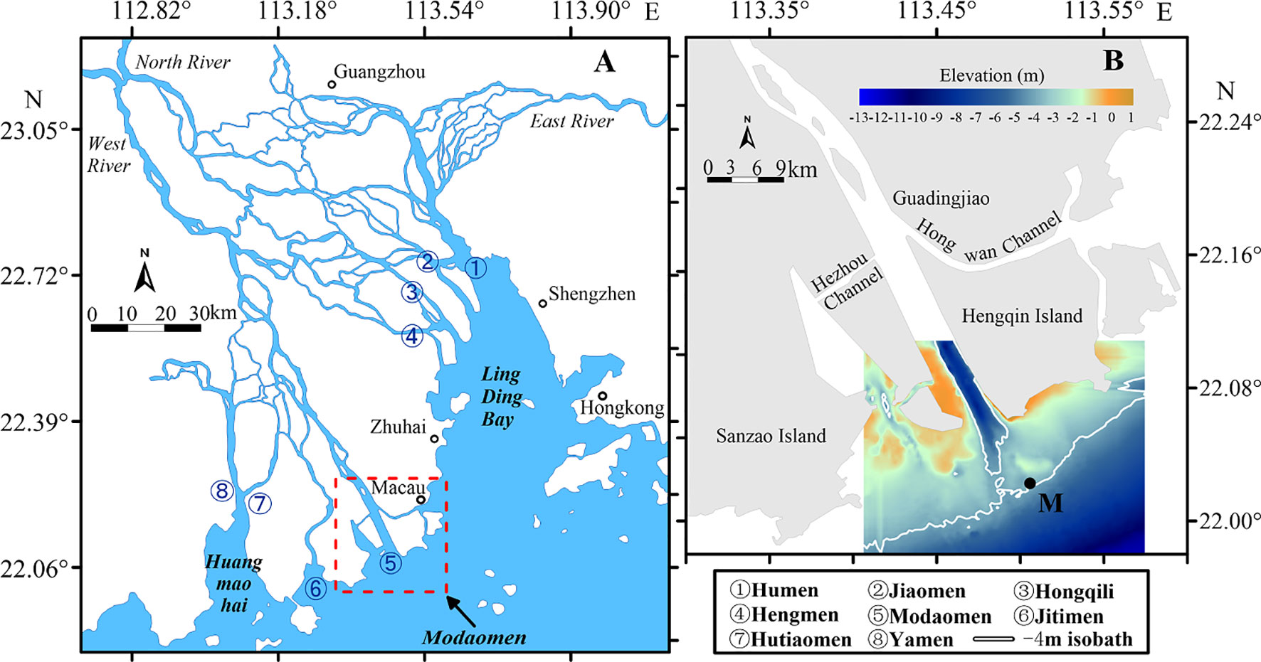
Figure 1 (A) Map of the Pearl River Estuary. (B) Map of the Modaomen Estuary, and the location of measurement site (M) in this study.
3 Materials and Methods
3.1 Field Investigation
In view of hydrodynamic characteristics during the dry season, both field shipboard and tripod investigations were simultaneously conducted at one site in front of the mouth bar of the Modaomen Estuary with an average depth of ~4.43 m over the dates of January 13–20, 2017, covering a full semidiurnal tide. The observation site M is located just in front of the central mouth bar (Figure 1B), which truly reflects complicated hydrodynamic conditions in the Modaomen Estuary, i.e., the intense saltwater intrusion, wave effects from the open ocean, and runoff scouring from upstream (Jia et al., 2015), and is an ideal site for field investigation to explore the effects of varying shear stresses and salinity stratifications on the vertical distribution of floc size. The shipboard observation system was used to measure a series of physical parameters, including velocity, salinity, temperature, turbidity, and floc parameters. An acoustic Doppler current profiler (ADCP, measurement accuracy: ± 2.5 mm·s-1; sampling rate: 0.1 Hz) was shipboard for continual vertical current structure data collection. An optical backscatterance sensor (OBS-3A, sampling rate: 1 Hz, hereafter OBS) was set to measure salinity, water temperature, and turbidity, which can be used to identify the location of the halocline by connecting to real-time transmitted data. A laser in-situ scattering and transmissometry instrument (LISST-100X Type C, sampling rate: 1 Hz, hereafter LISST) was deployed to record synchronous FSDs of volume-equivalent spherical particles in 32 logarithmically spaced size intervals covering the range 2.5–500 μm. The OBS and LISST were installed in a steel cage and set to record at hourly intervals. For data collection, the cage was slowly lowered from the surface to the bottom of the water column and then returned back to the surface. Water samples were collected every 1 or 2 h in three layers (i.e., surface, middle, and bottom layers) within the water column to calibrate the turbidity values collected by the OBS in the laboratory.
Simultaneously, a benthic tripod was deployed to the bottom at the sample site, M. An acoustic Doppler velocimeter (ADV, measurement accuracy: ± 1 mm·s-1) recorded three-dimensional (3D) current velocity and turbulence data at 0.3 m above the bed, which was sampled at 64 Hz in a 3-min burst every 10 min. The 3D current velocity data collected near the bottom boundary layer were considered to represent the timely turbulent flow intervention induced by the current–wave interaction, so that it could be applied to derive the turbulence shear stress (Safak, 2013; Ramírez-Mendoza et al., 2016).
3.2 Suspended Sediment Concentration Calibration
In this study, we retrieved SSC variations over the whole water column based on observation data from the OBS. For this, a timely OBS profile measurement was conducted from the surface to bottom water layer with a sampling frequency of 1 Hz, with in-situ sampling water of 1 L at the surface, middle, and bottom layers. Subsequently, a 0.45-μm glass fiber filter was used to filter water samples, and then samples were oven dried at 45°C for 48 h to determine the SSC. Regression analysis between measured OBS turbidity (NTU) and SSC values led to several linear relationships from spring, middle, and neap tides, respectively (Figure 2), which could then be used to convert the in-situ OBS turbidity data into SSCs. As shown in Figure 2, NTU data were well correlated (correlation coefficient R2 = 0.86, 0.84, and 0.75 at the spring, middle, and neap tides, respectively) with SSC (mg·L-1).
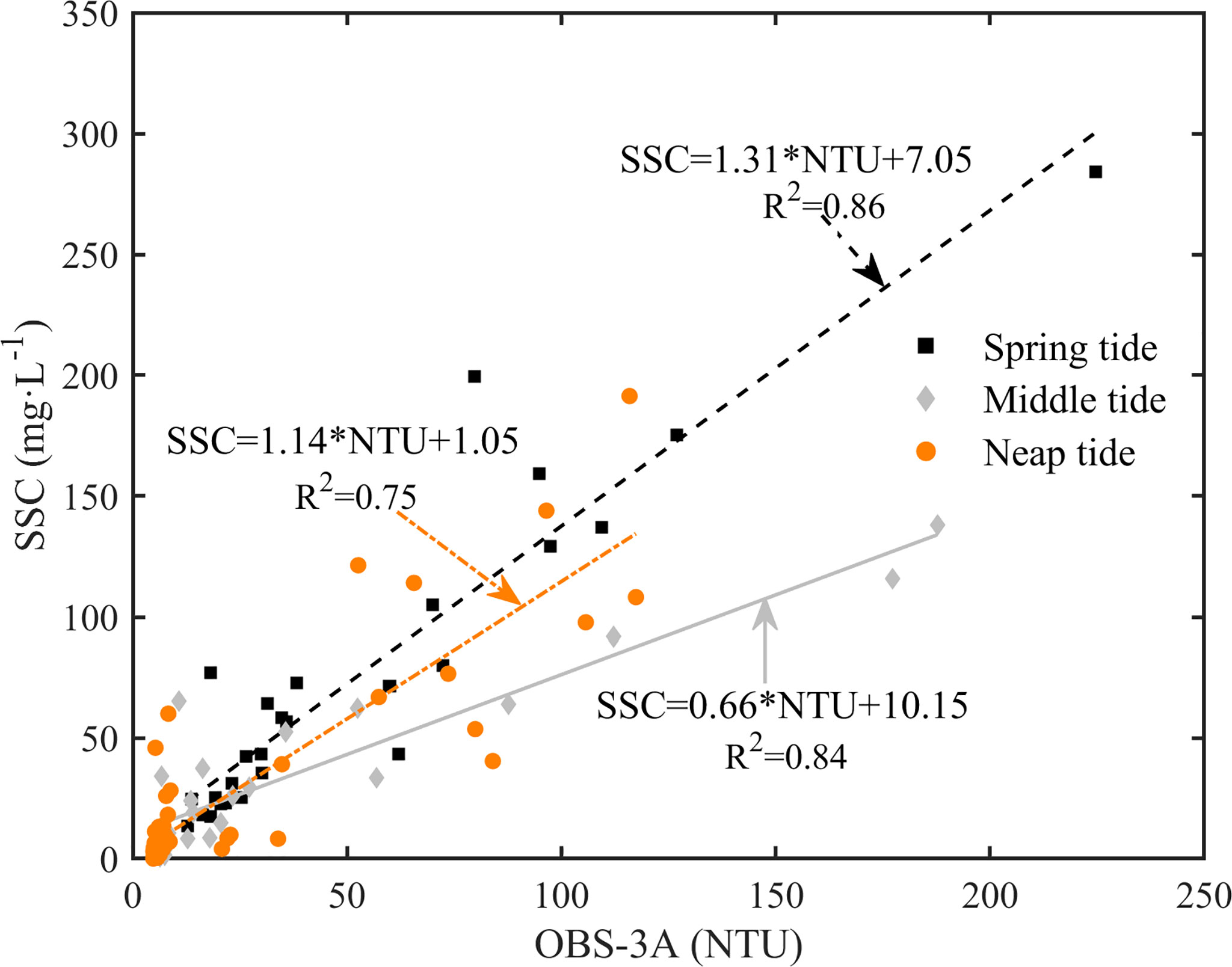
Figure 2 Calibration curves to derive suspended sediment concentration (SSC) from an OBS-3A.
3.3 Estimates of Shear Rate
In coastal or estuarine environments, turbulence plays a significant role in controlling the flocculation or deflocculation processes, promoting the aggregation by enhancing the colliding frequency of cohesive sediments or strengthening the breakup via breaking flocs apart (Mietta, 2010); therefore, it is necessary to estimate the effects of turbulence on flocculation processes. In this study, the shear rate (G) was estimated to explore the effects of turbulence; vertically, G is much stronger in the bottom layer compared with the value in the upper layer (Dyer and Manning, 1999; Wang et al., 2013).
G is defined by the turbulence dissipation rate (ε) as follows (Dyer and Manning, 1999):
with
where ν is the kinematic viscosity (1.026 × 10⁻⁶ m2·s-1, calculated by the measured temperature), κ is the von Karman constant (0.4), z is the height of the measurement sample volume above the bed, z = 0.3 m is used to calculate G as the bottom layer based on the ADV deployment location (Wang et al., 2013), and u∗ is the bottom friction velocity that is correlated with the bed shear stress (Soulsby, 1997):
where ρ is the density of seawater (1,017 kg·m-3, mean water density derived from the calculated salinity and SSCs) and τ is the shear stress.
The bed shear stress was derived from velocity profile data or turbulent flow theory based on the following independent methods: (1) the law of the wall (LP), (2) the Reynolds stress method (RS), and (3) the inertial dissipation method (ID) (Sherwood et al., 2006). The 3D velocity measured by ADV was dismantled into mean, wave, and turbulent components (Bian et al., 2018), where, without filtering the wave signals when processing with original turbulent flow data in order to retrieve the real τ, the RS method was used for estimating the bed shear stress τ using high-frequency instantaneous current velocity data from ADV as follows:
where ρ is the water density, and, u', v', and w', are the instantaneous turbulent components of the instantaneous velocity components (u, v, and w, respectively).
Importantly, the estimates of shear stress are highly dependent on the quality of the ADV measurements. Therefore, the ADV data should perform some pretreatments based on the results of previous studies to obtain useful data and ensure data quality (Yang et al., 2016; Peng et al., 2020). Initially, the parameters from the ADV tilt sensor should be analyzed in a unit of a single burst to ensure that the instrument maintains the correct gesture underwater, and the pitch and roll should be no more than 30°. Detecting the effective measuring data based on the correlation of acoustical signals and signal-to-noise ratio (SNR), the data of SNR lower than 20 dB and correlation smaller than 70% were removed (Nikora and Goring, 1999; Chanson et al., 2008). Furthermore, the rotation matrix (Equations (5), (6)) should be applied to rotate from the local ENU (east-north-up) coordinate system to the Cartesian coordinate system; thus, the previous measuring velocity data were Us = (ve, vn, vu) and after rotation was U = (u, v, w):
where θ is the vertical deflection angle and β is the horizontal deflection angle, about the determining of these two parameters, assuming that the velocity that is perpendicular to the main flow is zero therefore, the parameters can be defined as β = arctan(vn/ve), where vn is the northern component of velocity, ve is the eastern component of velocity, vu is the vertical component of velocity, and vs is the horizontal velocity that is defined as . Finally, the phase-space-thresholding (PST) method was used to replace burring data with the corresponding results of cubic polynomial fitting, and high-pass filtering (HPF) based on forward and inverse Fourier transform was used to obtain the data in the time domain. It should be mentioned that the signal of wave frequency was not filtered during the HPF process; therefore, the data subjected to the above calculations contained the information of both the current and wave dynamics, and hence the turbulent shear stress was a response to the real intricate environments.
3.4 The Difference of Potential Energy and the Standardization Stratification Coefficient
The difference in potential energy φ, as the qualification coefficient of water column stratification producing and disappearing, is the quantitative parameter of work that unit volume water converts from stratification to completely mixing condition (J·m-3); the degree of stratification is higher, and its value is larger, and with a more stable water column, which is defined as follows (Simpson et al., 1978):
where is the depth-averaged fluid density, ρi is the density of different layers, z is the height above the bed at different layers, and h is the depth (-h< z< 0). Here, the standardization stratification coefficient Sr was calculated, which is the dimensionless difference of potential energy, to eliminate the influence of depth on the estimation of the difference in potential energy (Li et al., 2018):
This coefficient represents the ratio of the energy required to mix the water column to the total potential energy; the larger the value, the stronger the stratification degree. Therefore, the degree of vertical mixing or stratification can be reflected through this ratio. Similar to other studies (Pritchard, 1955; Stacey et al., 2011; Pu et al., 2015), the value of Sr = 0.1% was the critical value of salinity-induced stratification in this study (Xie et al., 2021).
3.5 Decomposition of FSDs
Multimodal particle size distributions were decomposed to explore FSDs in this study. The FSDs are the sum of four lognormal distribution functions, defined as follows (Makela et al., 2000; Hussein et al., 2005; Lee et al., 2012):
where V and D are the volumetric concentration and diameter of each size interval of the LISST measured data, respectively; σi, , and represent the fitting characteristic parameter of each FSD and are the geometrical standard deviation, the geometrical mean diameter, which is equivalent to the median diameter (D50), and the volumetric concentration of the ith (i = 1, 2, 3, 4) unimodal FSD; and dV/dD represents the volumetric fraction normalized by the width of the size interval (Lee et al., 2012). Here, according to the observation, the median diameter of four fractions (primary particles, flocculi, microflocs, and macroflocs) was set to change as the curve-fitting parameter in the ranges of 0–4, 4–20, 20–200, and 200–1,000 μm, respectively. Besides, the upper bonds of standard deviation (σi) were confined under 3 to avoid unrealistically wide FSDs. The best-quality FSD provided characteristic parameter values of σi, , and for each subordinate lognormal FSD of four fractions. In this study, based on the LISST measured data of six characteristic layers, FSD decompositions were conducted to derive the four floc fractions and their spatiotemporal distributions.
4 Results
4.1 Hydrodynamic Changes
4.1.1 Velocity, Salinity, and SSC
Figure 3 shows the temporal changes in the vertical distribution of current speed, SSC, and salinity during the investigation periods. The current speed ranged from 0.024 to 0.699, 0.067 to 1.177, and 0.038 to 0.842 m·s-1, with average values of 0.330, 0.333, and 0.318 m·s-1 during the spring, middle, and neap tides, respectively (Figures 3A, D, G). It is clear that the speed value was larger in the surface layer than in the bottom layer, with a difference of 0.175 m·s-1 most of the time. During the spring tide, the semidiurnal tides were ebb-dominant and asymmetric, with a maximum depth-averaged ebb speed of 0.569 m·s-1 in the ebb peak flow period (Figure 3A).
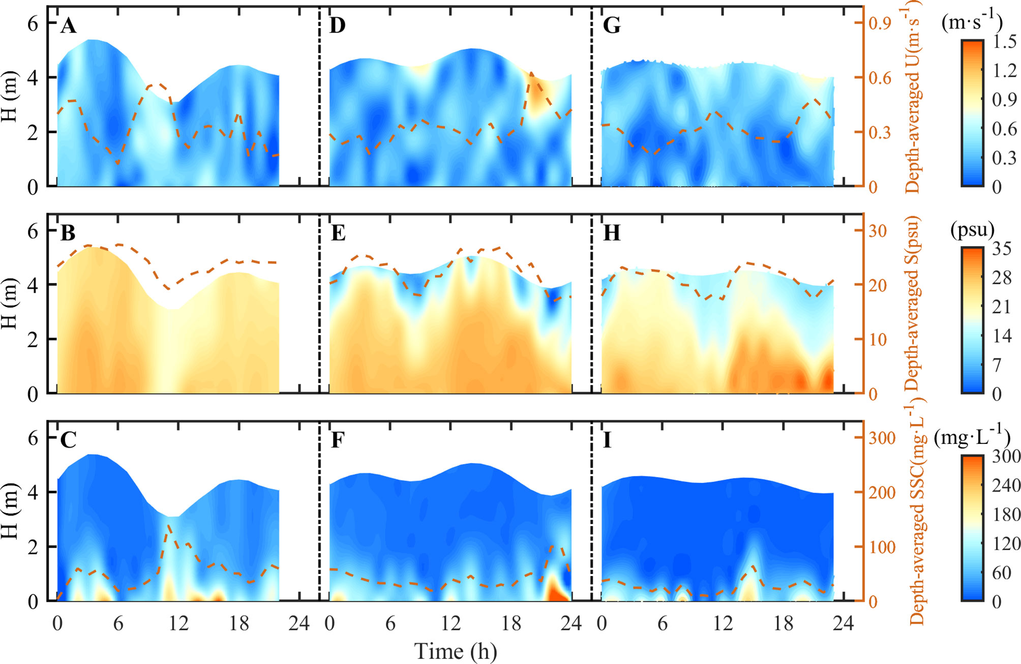
Figure 3 Vertical and temporal variation of (A, D, G) current speed (U, m·s-1), (B, E, H) salinity (S, psu), and (C, F, I) suspended sediment concentration (SSC, mg·L-1) at site M (A–C, D–F, G–I, represent the spring, middle, and neap tides, respectively). The orange dashed lines are temporal variations of depth-averaged U, S, and SSC.
The vertical distribution of salinity in the water column showed significant changes. The average vertical distribution of salinity ranged from 18.44 to 29.08, 2.80 to 29.86, and 5.43 to 30.56 psu during the spring, middle, and neap tides, respectively (Figures 3B, E, H). Vertically, distinct salinity-induced stratification was observed, especially during the middle and neap tides (Figures 3E, H). In general, salinity in the upper layer was lower than that in the bottom layer, with average salinity values of 11.88 and 14.01 psu in the surface layer and 28.33 and 28.24 psu in the bottom layer during the middle and neap tides, respectively.
The SSC ranged from 15.66 to 300.33, 13.06 to 448.92, and 5.37 to 253.33 mg·L-1 with average values of 61.65, 46.16, and 31.68 mg·L-1 during the spring, middle, and neap tides, respectively (Figures 3C, F, I). Similarly, the difference in SSC between the surface and bottom layers was obvious, the overall average SSC at the surface layer was 20.20 mg·L-1 and that at the bottom layer was 127.68 mg·L-1, and the maximum SSC (>300 mg·L-1) appeared during the ebb flow period in the spring tidal period, which was caused by the intense turbulent flow and sediment resuspension (Figure 3C). In general, a higher value of SSC was mostly observed at the bottom layer among all three tidal cycles (Figures 3C, F, I), indicating that the bed sediment source might have been caused by sediment resuspension.
4.1.2 Shear Rate and Salinity Stratification
Figure 4 shows the temporal changes in the turbulent shear rate (G) during the study period. The values ranged from 0.59 to 14.12, 0.39 to 16.30, and 0.07 to 17.69 s-1 with average values of 7.04, 8.65, and 5.47 s-1 during the spring, middle, and neap tides, respectively (Figures 4B, E, H). It is clear that the shear rate was the largest in the middle tides. The shear rate varied within the flood or ebb tides, and during the spring tide, the mean value of the flood tide was 8.33, which is evidently larger than the value of 5.86 during the ebb period. However, the flood tide values of 8.41 and 4.98 s-1 were lower than their counterpart ebb tide values of 8.95 and 5.88 s-1 during the middle and neap tides, respectively.

Figure 4 Vertical and temporal variation of (A, D, G) G (s-1), and temporal variation of (B, E, H) G in the bottom layer (s-1), (C, F, I) Sr (%); (A–C: spring tide; D–F: middle tide; G–I: neap tide). In the figures, the black dashed line (Sr = 0.1%) indicates the critical value of salinity stratification, the blue and orange dots represent the high shear rate with high SSC and the low shear rate with low SSC, respectively; and the blue and orange squares represent the high salinity stratification and low salinity stratification, respectively.
The Sr values ranged from 0.001% to 0.081%, 0.075% to 0.299%, and 0.092% to 0.248% with average values of 0.04%, 0.182%, and 0.168% during the spring, middle, and neap tides, respectively (Figures 4C, F, I). During the spring tide, strong tidal forces combined with runoff evidently led to vertical mixing, especially during the flood or ebb peak periods, yet also throughout the entire period with a low Sr value. However, the average value of Sr was greater than 0.1% in both the middle and neap tides, indicating intensive salinity stratification during those periods. Similarly, Sr fluctuated among the tidal cycles, with the average value of the flood tide Sr being 0.200%, which was larger than the value of 0.160% for the ebb during the middle tide, and likewise, the average value of flood tide Sr was 0.171%, also larger than the value of 0.166% for the ebb during the neap tide. Collectively, these values demonstrated a slight stratification degree with a value close to 0.1% when the speed was small during slack water periods (Figures 4F, I, 3D, G).
4.2 Median Size and Volume Concentration of Floc
In the lab, water samples can be used to retrieve dispersed particle size (d0) by the Mastersizer 3000 with Moment Method (John, 1988), and the measured particle median size (Md) was collected by the LISST-100C in the field measurement. Here, the ratio of Md to d0 was used to reflect the existence of the flocculation, and similar to the usage in other estuarine environments (Wang et al., 2016), in this study, this ratio was defined as the flocculation degree (DG = Md/d0). Generally, if the DG is higher than 1, it indicates that the dispersed particles are involved in the flocculation process.
Figure 5 shows the temporal variation of d0, Md, and DG in the surface, middle, and bottom layers during the study period, respectively. The value of Md ranged from 32.36 to 392.10, 22.13 to 380.35, and 3.37 to 337.42 μm in the surface, middle, and bottom layers, respectively (Figure 5); however, the value of d0 varied a little with the range of 8.57–41.16, 6.28–23.44, and 6.59–21.43 μm in each layer compared with the variation of Md. The trends of DG were highly synchronous with the variation of Md and the value of DG was all larger than 1, which means the flocculation process shown in the Modaomen Estuary every time within a different extent. Therefore, the data from the LISST-100X measurement were the true reflection of floc-size variation in the estuarine environment and the median measured particle size can be named as median floc size.
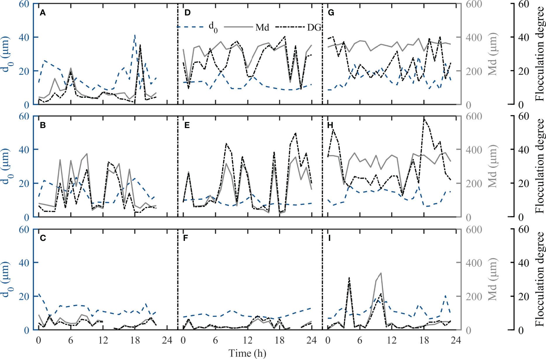
Figure 5 Vertical and temporal variation of median dispersed particle size (μm), median measured particle size (μm), and flocculation degree parameter (A–C, D–F, G–I, represent the spring, middle, and neap tides, respectively, A, D, G represent the surface layer, B, E, H represent the middle layer, C, F, I represent the bottom layer, the blue dash lines are the median dispersed particle size, the gray lines are the median floc size, and the black lines are the flocculation degree parameter).
Figure 6 shows temporal variations in floc volumetric concentration (Vc) and median floc size (Md) during the study period. The value of Vc ranged from 32.96 to 1,387.27, 25.38 to 1,476.43, and 20.43 to 1,490.09 μL·L-1 with average values of 345.84, 432.94, and 358.47 μL·L-1 during the spring, middle, and neap tides, respectively (Figures 6A, C, E). The maximum Vc value was 1,285.20 μL·L-1, corresponding with a large current speed (Figure 3A, 11–15 h), but the occurrence of its peak value lagged behind the appearance of the maximum speed. The depth-average values of Vc during the flood tide were 373.62, 461.17, and 373.06 μL·L-1 and were larger than those during the ebb tide with values of 320.76, 395.75, and 346.12 μL·L-1 during the spring, middle, and neap tides, respectively. The sediment trapping, occurring in the salinity stratification layer, undoubtedly increased the volumetric concentration, and the larger value in the bottom layer was likely caused by sediment resuspension. Consequently, the difference between the surface and bottom layers is more evident than that between other water layers in comparison, especially during the middle and neap tides, with the mean concentrations of 518.91 and 414.86 μL·L-1 at the surface layer and 631.94 and 472.32 μL·L-1 at the bottom layer, respectively.
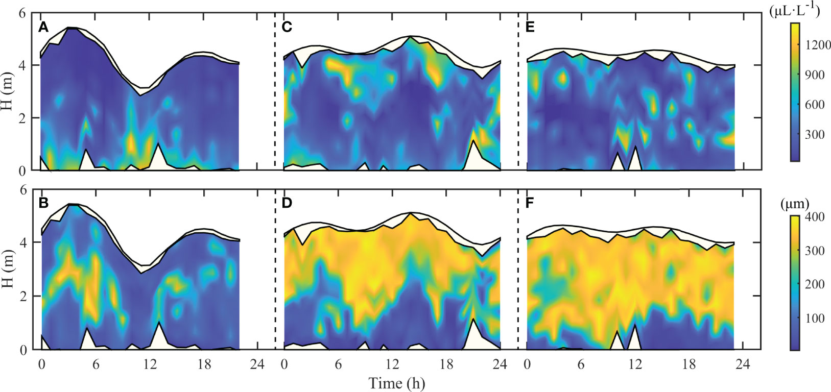
Figure 6 Vertical and temporal variation of (A, C, E) floc volumetric concentration (μL·L-1) and (B, D, F) median floc size (μm). (A–B, C–D, E–F, represent the spring, middle, and neap tides, respectively, and the white shadowed area represents the area for which no useful LISST data could be derived, due to high SSC values).
The value of Md ranged from 3.81 to 391.17, 3.37 to 410.83, and 4.58 to 392.10 μm with the mean values of 105.13, 210.22, and 259.71 μm during the spring, middle, and neap tides, respectively (Figures 6B, D, F). Md had a negative correlation with the current speed, and the breakup process was dominant during the peak flow period, causing the Md to be significantly smaller than that in slack water (Figures 3A, D, G, 6B, D, F). The smallest depth-average Md was 43.33 μm during the spring tide, compared with the values of 127.92 and 209.27 μm in middle and neap tides, respectively. In addition, the floc particles in the ebb-tide periods were mostly larger than those in the flood-tide periods during the three tides. Meanwhile, Md in the surface layer was evidently larger than that in the bottom layer, especially during the middle and neap tides, with values of 302.51 and 353.34 μm in the surface layer and 25.01 and 63.97 μm in the bottom layer, respectively. The strong turbulence shear stress caused the breakup process to be dominant, resulting in a smaller floc size, even if supplied with a large amount of resuspended sediments (Figures 3F, I).
4.3 Variations in FSDs
4.3.1 Decomposition in the Characteristic Tide Level
The floc sizes at the characteristic tide level, including flood peak and slack, and ebb peak and slack, were decomposed, and the results are shown in Figure 7. During the spring tide, depth-average floc sizes were 46.01 and 32.32 μm in flood (1 h) and ebb (10 h) peak flows, respectively, and decomposed into the four types: Pp, Flocculi, Micro, and Macro. The four floc types accounted for 27.98%, 10.02%, 42.19%, and 19.81% in the flood peak flows, and 44.66%, 9.45%, 40.76%, and 5.13% in the ebb peak flows, respectively with Pp and Micro flocs being dominant. In comparison, the depth-averaged floc size was larger with values of 73.91 and 58.54 μm in slack water periods (5 and 12 h, respectively), and with the four floc types accounting for 11.84%, 10.2%, 46.69%, and 31.27%, and 30.8%, 5.06%, 43.02%, and 21.11%, respectively. From this, the concentration of Micro was more evident, and Pp was relatively smaller but still significant than in peak flows. Vertically, the FSDs were highly consistent in a bimodal pattern with Pp and Macro being dominant in peak flow periods (Figures 7A, G); in contrast, the FSDs of the surface and middle layers were skewed toward larger sizes, but smaller flocs became more evident in the bottom layer in slack flow periods (Figures 7D, J). Overall, the FSDs in the spring tide were broader and even among the diameter range of 10–100 μm compared with the middle and neap tides.
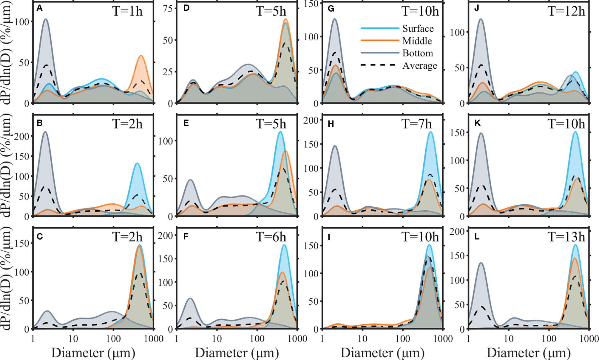
Figure 7 Normalized measured FSDs among the water column (black dash lines) and surface (blue lines), middle (orange lines), and bottom (gray lines) layers and characteristic times; (A, D, G, J), (B, E, H, K), and (C, F, I, L) represent the spring, middle, and neap tides, respectively; (A–C) show the flood peak flow, (D–F) show the flood to ebb slack water, (G–I) show the ebb peak flow, and (J–L) show the ebb to flood slack water. Here, dp/dln(D) is the volumetric percentage normalized by the width of the size interval on the log scale.
Similarly, during the middle tide, the FSDs were composed of different characteristic tidal levels with the four types of flocs, accounting for 29.27%, 11.57%, 14.92%, and 44.24% in peak flow (Figures 7B, H), and 21.06%, 11.8%, 18.04%, and 49.1% in slack water (Figures 7E, K), respectively. However, with the occurrence of strong salinity-induced stratification (Figures 3E, 4F), the decomposition varied considerably vertically. The surface layer was a macro-dominant single peak with an average diameter of 430.65 μm and dramatically accounted for 89.96% based on the four tidal levels. In the middle layer, the FSD was shaped in a three-peak pattern with Pp, Micro, and Macro being dominant, and Macro being the most dominant, accounting for 48.61% in slack water (5 h, 10 h), which was larger than the value of Macro (34.69%) in the peak flow period (2 h, 7 h). Affected by the long duration of turbulent shear stress (Figure 4E), the bottom layer was still a Pp significant single peak accounting for 63.33% with flocs mostly smaller than 10 μm in the peak flow, but changed in a dual-peak tendency with the increase of Micro in slack water.
During the neap tide, the FSDs were almost unimodal, with the four types of flocs accounting for 5.46%, 8.05%, 14.49%, and 72%, respectively, during the peak flow period (2 and 10 h), and 18.96%, 6.28%, 11.56%, and 63.19%, respectively, in slack water (6 and 13 h). Macro was dominant even at different tidal levels, but the concentration was more evident in the peak flow due to the unimodal FSD in the bottom layer of the ebb peak flow (Figure 7I). With the subsidence of the salinity stratification interface (Figure 3H), the FSD changed significantly vertically. The surface and middle layers were single-peak structures with Macro dominance, accounting for 85.12% of peak flow, and similarly, the unimodal pattern with Macro dominance in slack water was even larger, accounting for 91.43%. In the bottom layer, the FSD was bimodal in shape with Pp and Micro both being evident in the flood peak flow (Figure 7C), but this transformed into a Macro-dominant single peak in the ebb peak flow (Figure 7I), and FSD also skewed left with the decrease in Macro and increase in Pp or Micro in slack water.
4.3.2 Vertical and Tidal Variations in FSDs
Figure 8 shows temporal variations in volumetric concentrations of the four floc size fractions, that is, Pp, Flocculi, Micro, and Macro during the spring, middle, and neap tides. According to the decomposition results, the volumetric concentration of Macro and Pp was larger, with overall average values of 315.50 and 115.95 μL·L-1, followed by Micro with a mean value of 109.38 μL·L-1, and the minimal volumetric concentration of Flocculi with a mean value of 38.30 μL·L-1.
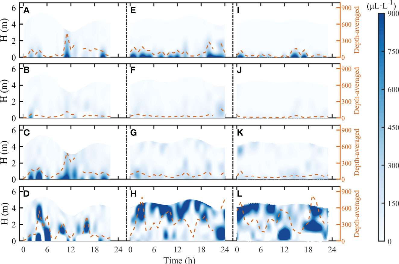
Figure 8 Vertical and temporal variation of volumetric concentration of primary particles (Pp, A, E, I), Flocculi (B, F, J), microflocs (Micro, C, G, K), and macroflocs (Macro, D, H, L). (A–D, E–H, I–L, represent the spring, middle, and neap tides, respectively) at site M. The orange dashed lines are the temporal variations of the depth-averaged volumetric concentration (μL·L-1).
The volumetric concentration of the finest flocs, Pp, ranged from ~0 to 1,257.18, ~0 to 1,586.07, and ~0 to 1,314.12 μL·L-1 with depth-average values of 135.49, 142.02, and 70.65 μL·L-1 during the spring, middle, and neap tides, respectively (Figures 8A, E, I). A higher volumetric concentration of Pp was detected in the bottom layer with average values of 580.55, 709.94, and 393.74 μL·L-1 in each tidal period, respectively, and the maximum concentration appeared in the first flood peak flow of the middle tide at 2 h (Figure 8E). During the spring tide, the largest value was shown in the first ebb to flood slack water at 12 h and the lowest value occurred in the first flood to ebb slack water at 5 h. During the middle tide, the maximum value occurred at the first flood peak flow at 2 h, but the minimum value was observed at 19 h. During the neap tide, at 16 h, the volumetric concentration of Pp was the largest, compared with its lowest value, shown at 3 h.
Flocculi smaller than 20 μm, as another component of the unbreakable flocs in the flocculation process, had the lowest values among the four fractions and showed relatively weak variation. The volumetric concentration of Flocculi ranged from 0.03 to 232.17, 1.04 to 371.23, and 5.63 × 10⁻³ to 155.94 μL·L-1 with the depth-averaged values of 46.19, 47.09, and 21.76 μL·L-1 in the spring, middle, and neap tides, respectively (Figures 8B, F, J), with the neap tide having a distinctly lower value. Similar to the distribution of Pp, more Flocculi particles aggregated in the bottom layer, with mean values of 106.82, 106.65, and 75.49 μL·L-1 in the spring, middle, and neap tides, respectively, and the Flocculi volumetric concentration varied frequently accompanied by most of the extremum shown in this layer; the maximum value of Flocculi occurred at 4, 22, and 13 h, and the minimum values were located at 14, 2, and 16 h in the spring, middle, and neap tides, respectively.
For Micro, which generally ranges from 50 to 200 μm, the distribution was highly consistent with the variation of Pp vertically, especially during the spring tide. The volumetric concentration of Micro ranged from 10.04 to 933.89, 4.04 to 424.69, and 1.80 to 477.72 μL·L-1 with depth-average values of 165.83, 94.85, and 70.60 μL·L-1 during the spring, middle, and neap tides, respectively (Figures 8C, G, K). The observed size of Micro was consistent with the surface sediment particle size in the central mouth bar that is approximately 3–5 φ (Chen et al., 2017), and the distribution pattern of Micro was similar to the suspended sediment concentration distribution pattern (Figures 3C, F, I), which suggests that Micro may be attributed to both sediment resuspension and flocculation processes, as is demonstrated by the maximum value shown at 9 h in the spring tide. Micro was dominant in the bottom layer, with average values of 388.77, 230.18, and 198.40 μL·L-1, respectively, among the three tidal cycles, and the concentration of Micro during the spring tide was significantly larger than that of the other two tides. The extremum was not bounded at the bottom layer, the maximum value of each tide occurred at 9, 23, and 0 h, and the minimum values occurred at 20, 7, and 8 h, respectively.
The largest fraction of Macro floc particles, larger than 200 μm, presented different distribution characteristics compared with the three fractions mentioned previously. The value of Macro ranged from 12.99 to 2,258.73, 11.58 to 2,043.70, and 6.75 to 1,953.24 μL·L-1 with depth average values of 158.88, 399.48, and 378.72 μL·L-1 during the spring, middle, and neap tides, respectively (Figures 8D, H, L), suggesting the largest volumetric concentration within four fractions. In contrast, Macro was extremely evident in the middle and neap tides, but less evident in the spring tide. In the spring tide, a lower value of 46.47 μL·L-1 occurred in the surface layer compared with the increasing value in other layers, so the lowest value occurred in the shallow depth layer at 20 h and the largest occurred in the deep depth layer at 5 h. Contrarily, Macro fluctuated more frequently in the shallow-depth column and the volumetric concentration was more evident in the upper and middle layers than in the others; the maximum value was observed at 21 and 0 h, and the minimal value occurred at 14 and 1 h in the middle and neap tides, respectively.
5 Discussion
5.1 Flocculation and Deflocculation Processes
According to the decomposition results of FSDs in the Modaomen Estuary, temporal variations in Pp, Flocculi, Micro, and Macro in the water column (surface, middle, and bottom layers) during different tidal cycles are shown in Figure 9. Vertically, the percentage of Pp increased from the surface layer with a mean percentage (of the three tides) of 5.96% to the bottom layer with a mean value of 44.38%, and the percentage of Micro also increased from 18.67% to 30.20%; in contrast, the largest fraction of Macro evidently decreased from 68.19% to 14.85%. Strong turbulent flow contributed to the dominant deflocculation process in the bottom layer, and flocs frequently exchanged between the Pp and Micro fractions, with the floc median size dramatically decreasing from 249.14 μm in the surface layer to 44.50 μm in the bottom layer. Similarly, at specific moments, the floc breakup was dramatic and their median size was even smaller than 10 μm when the turbulent stress reached its maximum value (Figure 4B), and the percentage of the Pp fraction increased sharply to 81.40% while that of Micro decreased to 6.46%, with the percentages of Flocculi and Macro being 5.56% and 6.58% (Figure 9C, 15 h), respectively. However, intensive flocculation processes were detected during the neap tide, past the 4-h mark, with proper turbulence shear (near 5 s-1) and the dropping of salinity, from 27 to 23 psu, which enhanced the collision frequency among particles, making it easier to format the larger floc particles within a loose structure (Mietta, 2010). Therefore, the percentage of Macro rapidly increased to 89.51% in several hours, and other components that comprised less than 5% of the particles were involved in the flocculation process (Figure 9I, 6–10 h). After this period, floc particles gradually broke up with the increase in turbulent shear, and Pp became dominant again with an average value of approximately 41.40% (Figure 9I).
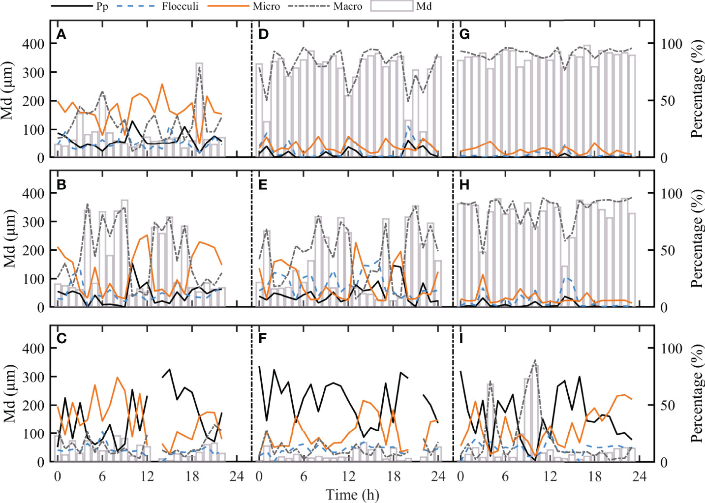
Figure 9 Temporary variability of the floc size (μm), volumetric percentage of Pp, Flocculi, Micro, and Macro in the surface layer (A, D, G), middle layer (B, E, H), and bottom layer (C, F, I). The gray bar indicates the floc size based on the left scale and several broken lines; the black lines are Pp, the blue dashed lines are Flocculi, the orange lines are Micro, and the gray lines are Macro, all based on the right scale (A–C, D–F, G–I represent the spring, middle, and neap tides, respectively.
As shown in Figure 9, floc fractions and median floc size varied among the different layers, reflecting unequal flocculation and deflocculation processes. In the surface layer, the flocculation process was extremely obvious with a median floc size greater than 200 μm, and the percentage of Macro was nearly larger than 80%, except during the spring tide. Affected by the strong bio-flocculation process (Li et al., 2017), smaller particles such as Pp and Flocculi that function as building blocks were highly engaged in producing larger, loose flocs, and salinity stratification led to longer residence times of the larger flocs in the surface layer. In the middle layer, with the intensive salinity-induced stratification, sediment was effectively trapped in this layer, supplying more smaller particles for the formation of larger flocs (Ren and Wu, 2014; Zhang Y, et al., 2021), thereby causing flocs to exchange frequently between the Micro and Macro factions. During the neap tide, within the halocline, floc particles were still large with a mean value of 327.98 μm and the percentage of Macro was 85.49%, which exceeded the percentage of other floc fractions. However, in the bottom layer, deflocculation processes were extremely evident; most of the median floc size was even lower than 50 μm and Pp was dominant in each tide with mean percentages of 39.22%, 54.70%, and 38.78%, respectively. From this, it can be said that both the effective turbulent flow and trapping effects of the halocline contributed to the intense deflocculation process in the bottom layer, mostly leading to the exchange between Pp and Micro.
5.2 Influencing Factors
5.2.1 Effects of Hydrodynamic Factors
Previous studies have indicated that SSCs, salinity, and turbulent shear stress affect the flocculation and deflocculation processes, which determine the floc size distribution (Guo et al., 2018; Deng et al., 2019; Byun and Son, 2020; Li et al., 2021; Zhang Y, et al., 2021; Zhang et al., 2020). Figure 10 displays the irregular and complicated quadratic fitting correlations between G, SSC, and S and the volumetric concentrations of Pp, Flocculi, Micro, and Macro at the bottom layer, during the spring, middle, and neap tides. The results indicate that, among the four floc fractions, Pp and Micro changed the most in response to the variation in environmental parameters but did not follow a regular pattern. Compared with the two frequently exchanged fractions, Flocculi and Macro maintained a constant level with a nearly unvaried trend as compared with the variation of all mentioned factors.
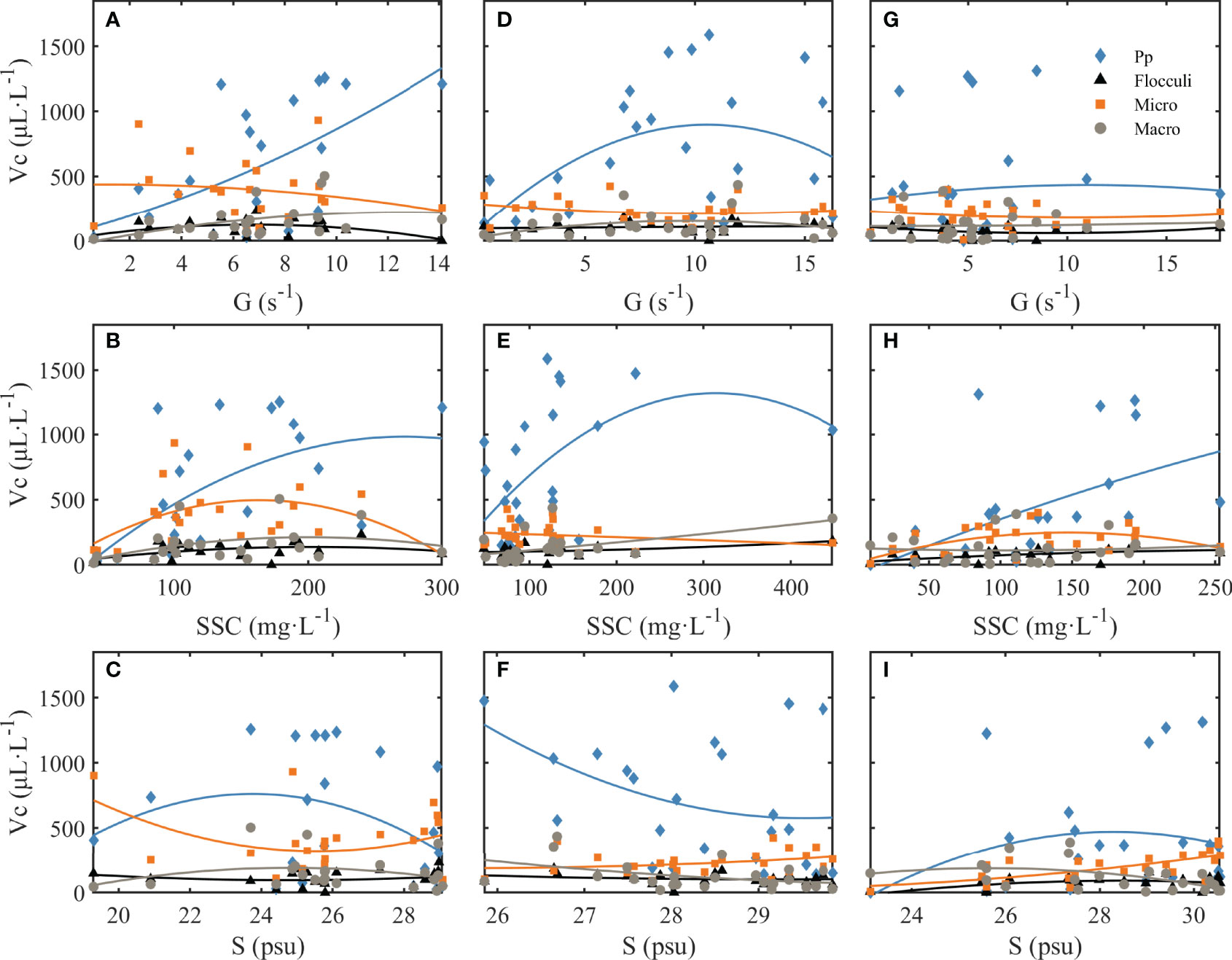
Figure 10 Scatter plots of (A, D, G) turbulent shear rate G (s-1), (B, E, H) SSC (mg·L-1), (C, F, I) S (psu), and volumetric concentration of Pp, Flocculi, Micro, and Macro (A–C, D–F, G–I represent the spring, middle, and neap tides, respectively).
Flocs exchanged frequently between Pp and Micro with the variation of turbulent shear rate (G), but Flocculi and Macro flocs changed only slightly. Pp showed an obvious positive correlation with the increase in G, especially during the spring tide (Figure 10A), but tended to decrease when G was more than 10 s-1 in the middle tide (Figure 10D) and presented a constant trend during the neap tide (Figure 10G). Typically, strong turbulent flow can be expected to lead to intense sediment resuspension as these two factors change synchronously. This was seen in the results, in that the correlation between SSCs and floc fractions (Figures 10B, E, H) was almost the same as that of G. In contrast, during the spring and neap tides (Figures 10C, I), small factions of Pp first increased and then decreased with the increase in salinity (S), whereas in the middle tide (Figure 10F), Pp decreased monotonically, accompanied by the variation of S. In addition, larger flocs, such as Micro, presented an obvious contrary correlation compared with the variation of Pp. Typically, the increase of minor particles (Pp) reflects the evident deflocculation processes and vice versa, but in this study, the correlation stated above indicated an irregular flocculation process, that is, Pp first increased and then decreased, which is inconsistent with the pattern identified for tide-dominant environments (Zhang et al., 2020).
Considering the complexity of multiple factors influencing the environment, certain extreme cases (see times indicated by the markers in Figure 4) were selected to more closely investigate the influences of two key factors, turbulent shear rate (G) and salinity-induced stratification (Sr), on floc size distribution, as discussed in Sections 5.2.2 and 5.2.3. To achieve this, all non-discussed factors were controlled at an ordinary or low level.
5.2.2 Impact of Turbulent Shear Stress
Figures 4A, D, G show the vertical distribution of G for spring, middle, and neap tides, respectively. G had high values in periods of peak flow and was extremely high in the bottom layer, which was consistent with the occurrence of smaller flocs in the bottom layer (Figure 8). Moreover, it tends to be low near the surface layer, corresponding to the existence of Macro. In addition, the effects of extremely high or low turbulent shear stress on the distribution of the four floc fractions could be identified by the decomposition of the FSDs. Figures 11A, C, E present entirely different FSDs at different layers with higher turbulent shear; the FSDs showed a multimodal pattern with coarser flocs being dominant at the surface layer, mostly with particle sizes between O (10) and O (100). This changed, with the floc size increasing to O (100) with macro-dominant unimodal FSD at the middle layer; the FSD of Pp was considerably dominant at the bottom layer with floc size confined to O (1), indicating that the deflocculation process was dominant. In weak turbulent shear that actually existed in the slack tide period, the FSD of coarser particles was more dominant at the surface and middle layers, with the narrow range of particle sizes being significantly larger than O (100) with a Macro-dominant unimodal pattern (Figures 11B, D, F). Finally, the FSD was multimodal with Pp and Micro being dominant at the bottom layer, with floc aggregation being affected by the breakage, and floc size varied intensely from O (1) to O (100).
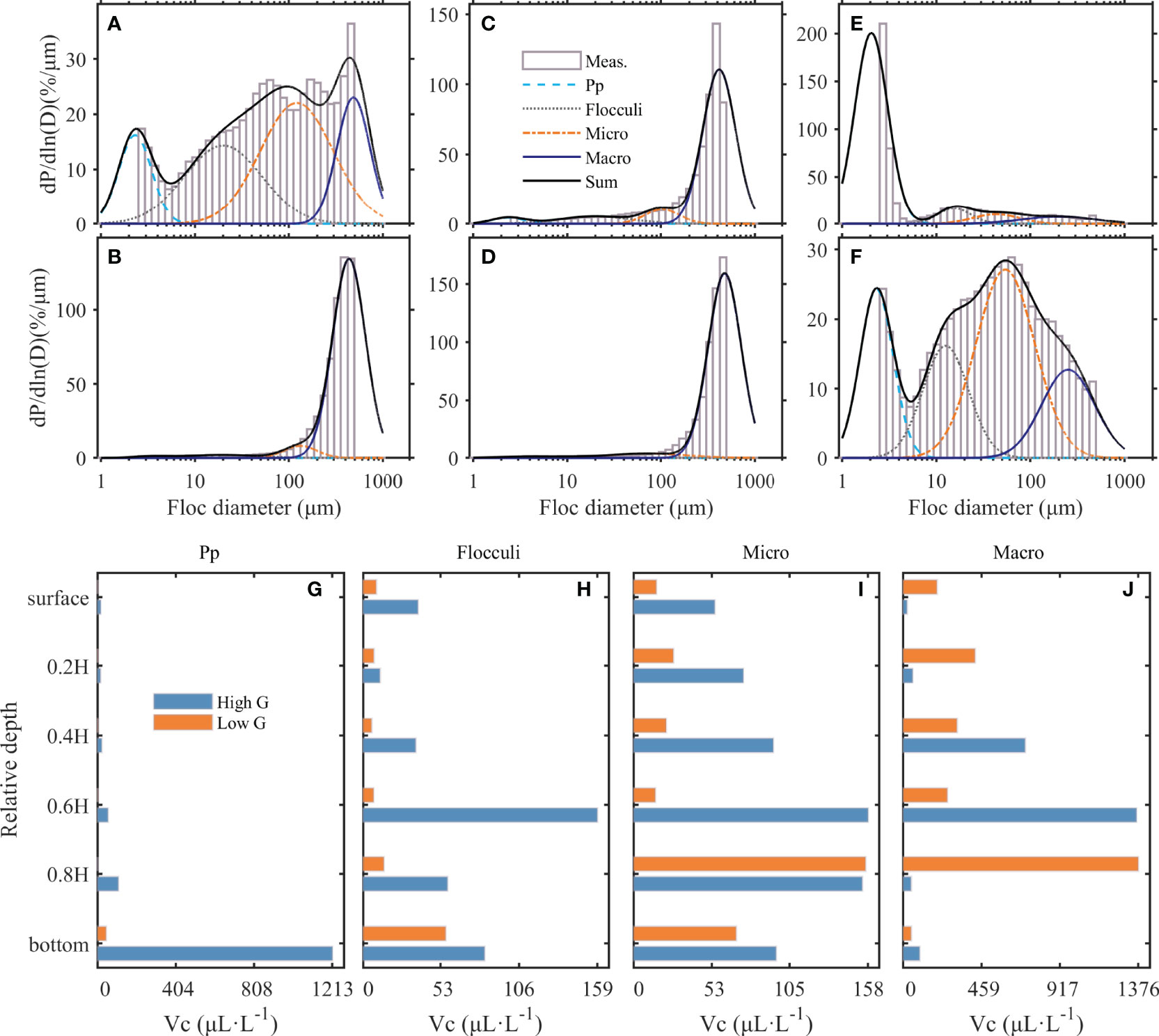
Figure 11 (A, C, E) FSDs at the surface, middle, and bottom layers within high turbulent shear and SSC conditions (High G, shown in Figures 4B, C, the blue dots); (B, D, F) FSDs at the surface, middle, and bottom layers within low turbulent shear and SSC conditions (Low G, shown in Figures 4H, I, the orange dots). Meas. presents a FSD measured by the LISST instrument, and Sum indicates the superposition of the decomposed FSDs. (G–J) Different floc fraction volume concentration variation in the relative depth from the surface layer to the bottom layer, and H in High and Low G conditions were 4.05 and 4.48 m measured by the ADCP, respectively.
To analyze this in more detail, the vertical volume concentration variations were investigated among four fractions (Pp, Flocculi, Micro, and Macro, Figures 11G–J). Affected by high shear and SSCs, the volume concentration of Pp in the bottom layer was larger than that of any other flocs and evidently larger than the value at low shear and SSCs (Figure 11G). The high shear and SSCs were related to sediment resuspension, leading to the Flocculi having a maximum value at the 0.6 H layer, and the whole water column remained at a consistent concentration, which was affected by low turbulent shear (Figure 11H). The larger and loose floc modes, Micro and Macro, showed similar vertical distribution patterns: the peak of volume concentration occurred in the 0.8 H layer when turbulent shear and SSCs were lower but occurred in the shallow 0.6 H layer with higher turbulent shear and SSCs. Higher turbulent shear with stronger vertical mixing and strong sediment resuspension then occurred, causing Micro to translate upward, closer to the middle layer, or causing Macro to either break up within the upper layers and translate into the near bottom layer to supplement the finer flocs or ultimately deposit in low shear and SSC conditions (Figures 11I, J).
The effects stated above support the concept that the turbulent shear mainly controls the flocculation and deflocculation processes at the bottom layer and is consistent with the typical turbulent shear-dependent theory; the underlying layers are affected by dozens of factors, such as stratification, salinity, or bio-activities (Li et al., 2017; Zhang Y, et al., 2021). In the bottom layer, Pp synchronously fluctuated with turbulent shear and exchanged with Micro, and the variations of coarser flocs, such as Flocculi and Micro, are strongly related to sediment resuspension. This last holds true except in regard to the flocculation or deflocculation process, wherein the turbulence may have a weak effect on the variation of Macro; within weak turbulent shear, largest flocs could exist in bottom layers (0.8 H) which may be due to fast settling of flocs from upper layers, but Macro cannot be the single dominant group in the bottom layer due to its tendency to break up caused by turbulent effects and its fragile loose inner structure. In this study, it seems that turbulent shear was not the sole factor controlling different floc size distributions beyond the bottom layer, which can also be affected by flocs settling in the water column.
5.2.3 Impact of Salinity Stratification
Figure 12 shows the distinctive decomposition of FSDs at different layers when the salinity stratification was strong or weak. According to the vertical variation of salinity (Figure 12K), a dramatic change was observed around the 0.6 H layer (middle layer), indicating the occurrence of strong salinity-induced stratification. At the surface layer, the FSD was a coarse-unimodal (O (100)) pattern with Macro dominance (Figure 12A). Around the halocline, the FSD was consistent with the upper layer present in a macro-dominant unimodal (O (100)) pattern (Figure 12C). However, at the bottom layer, the FSD converts from a unimodal to a multimodal pattern with Pp and Micro being dominant with a particle size range between O (1) and O (10) (Figure 12E), which follows the typical turbulent shear-dependent theory. On the contrary, affected by strong turbulent vertical mixing, the FSDs maintained a rather consistent multimodal pattern with Pp and Micro being dominant with a wider range of flocs between O (1) and O (10) that changed only in magnitude; Pp was more evident than Micro at each of the different layers, especially at the bottom layer (Figures 12B, D, F).
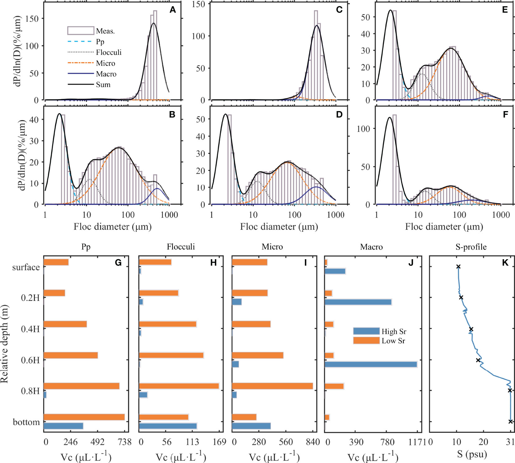
Figure 12 (A, C, E) FSDs at the surface, middle, and bottom layers with strong salinity stratification (High Sr, shown in Figures 4H, I, the blue squares); (B, D, F) FSDs at the surface, middle, and bottom layers with strong vertical mixing (Low Sr, shown in Figures 4B, C, the orange squares). Meas. presents a FSD measured by the LISST instrument, and Sum indicates the superposition of the decomposed FSDs. (G–J) Different floc fraction volume concentration variations in the relative depth from the surface layer to the bottom layer; and H in High and Low Sr conditions were 4.10 and 3.33 m measured by the ADCP, respectively. (K) Salinity profile in the strong salinity stratification.
By investigating the floc size distribution throughout the water column, evident differences were indicated by two distinct degrees of stratification. Figures 12G–K show the volume concentration of the finer flocs, Pp and Flocculi, within clear salinity stratification, which maintained a low concentration from the surface to the 0.8 H layer and then reached a higher value at the bottom layer (Figures 12G, H). However, when vertical stratification mostly disappeared, the volume concentration dramatically increased and was larger than the value in the previous strong salinity stratification conditions. Flocculi generally vertically increased from the surface to the bottom layer but also presented a high-value bulge at the 0.8 H layer (Figures 12G, H). Micro maintained an analogous distribution as Pp and Flocculi under strong salinity stratification conditions. In addition, under the significant vertical mixing, the convex of vertical distribution of Micro at the 0.8 H layer was more evident and the value was even higher beneath that depth; the occurrence of this high value peak may have resulted from the strong sediment resuspension (Figure 12I). In contrast, the vertical distribution of Macro within the two cases was inverted, and the volume concentration of Macro with strong turbulent mixing maintained a vertically consistent but low value pattern. In contrast, Macro showed an evident variation of vertical distribution, within strong salinity stratification, in that extremely high values appeared at both the 0.2 H and 0.6 H layers and lower concentrations appeared at the other layers (Figure 12J).
The barricade of the salinity halocline was expected to block the vertical exchange of flocs by trapping sediment (Wu et al., 2012; Ren and Wu, 2014) and finer flocs, thereby strengthening the flocculation process with Macro becoming dominant near the stratification layer (0.6–0.8 H) and leading to different flocculation mechanisms at different layers of varied turbulent flow. The bulge of Macro near the surface layer may have resulted from strong biological activities and could have been supported by the presence of organisms or transparent exopolymer particles within the freshwater (Li et al., 2017; Li et al., 2021; Fettweis et al., 2022). Under conditions of strong vertical mixing, whether the flocculation or deflocculation process became dominant mainly depended on the extent of the turbulence shear; this was demonstrated by the flocs frequently exchanging between Pp and Micro sizes, which means smaller flocs could also concentrate in the surface layer and be one of the dominant groups affected by vertical sediment diffusion.
6 Conclusions
This study explored temporal and vertical changes in floc size distribution and their influencing factors during the dry season in the Modaomen Estuary. The decomposition results of the FSDs revealed that the four floc fractions exhibit huge spatiotemporal variability. The finest fraction, Pp, commonly concentrated at the bottom layer, especially at several peak flow periods. The mixed-size fraction, Flocculi, had a high concentration at the bottom layer, but varied slightly. Micro had a particle size consistent with surface sediment particles; thus, it had an agreed distribution pattern with suspended sediment concentration, with higher concentrations of Micro at the bottom layer. In contrast, the largest floc fraction, Macro, showed inconsistent distribution among the whole water column but was mostly concentrated in the upper and middle layers with some scattered distribution at the bottom layer.
Additionally, the single-factor analysis was ambiguous, while the antagonistic dynamic scenarios identified that the floc size distribution in the upper layer was controlled by Macro and the salinity stratification in the middle layer was the main contributor to the larger flocs, which turned shear-dependent in the bottom layer. The FSDs in the upper or middle layers skewed toward a larger particle size with single peaks and lack of exchange among the different floc fractions, leading to micro-dominance with a larger volume concentration and median size which impeded vertical mixing by salinity stratification. However, the FSDs in the bottom layer skewed toward a smaller particle size with a dual-peak tendency, and floc particles frequently exchanged between Pp and Micro.
The Pp particle size was dominant under strong turbulent shear stress conditions and showed an evident deflocculation process. The volume concentration of Micro was enhanced by sediment resuspension, whereas Pp converted to Micro significantly under conditions of low turbulent shear, with the flocculation process being dominant. In addition, stronger turbulent flow was seen to strengthen the vertical mixing of the water column, causing the fast deposition of Macro and breaking down of Macro into Micro. In particular, at the bottom layer, the decrease in salinity was the main contributor to the formation of Macro, which was supported by smaller flocs, but Pp was dominant overall and larger flocs could not be restricted under high-salinity conditions.
Data Availability Statement
Most of the datasets used in this article can be found at http://dx.doi.org/10.17632/r9nzmjdfzx.3, an open access online data repository hosted at Mendeley Data (Huang, Jie, “Effects of shear stress and salinity stratification on floc size distribution during the dry season in the Modaomen Estuary of the Pearl River: Datasets”, 2022, Mendeley Data, V3).
Author Contributions
JH: formal analysis, figure drawing, writing (original draft). SW, XL: software, data checking. RX, JS: turbulence data processing. FL: supervision, funding acquisition, and writing (review and editing). BS, HC, QY, ZZ: writing (review). All authors contributed to the article and approved the submitted version.
Funding
This research was financially supported by the Open Research Fund of State Key Laboratory of Estuarine and Coastal Research (Grant No. SKLEC-KF202101), the National Natural Science Foundation of China (Grant Nos. 42076171, 41706088), the Guangzhou Science and Technology Program of China (Grant No. 202102020450) and the Marine Economic Development Project of Guangdong Province (Grant No. GDNRC[2020]050).
Conflict of Interest
The authors declare that the research was conducted in the absence of any commercial or financial relationships that could be construed as a potential conflict of interest.
Publisher’s Note
All claims expressed in this article are solely those of the authors and do not necessarily represent those of their affiliated organizations, or those of the publisher, the editors and the reviewers. Any product that may be evaluated in this article, or claim that may be made by its manufacturer, is not guaranteed or endorsed by the publisher.
Acknowledgments
We deeply acknowledge the reviews for their valuable comments and suggestions and would like to thank Dr. Leiping Ye for useful suggestions on the decomposition of floc size distribution.
References
Aagaard T., Hughes M., Baldock T., Greenwood B., Kroon A., Power H. (2012). Sediment Transport Processes and Morphodynamics on a Reflective Beach Under Storm and non-Storm Conditions. Mar. Geol. 326, 154–165. doi: 10.1016/j.margeo.2012.09.004
Bian C., Liu Z., Huang Y., Zhao L., Jiang W. (2018). On Estimating Turbulent Reynolds Stress in Wavy Aquatic Environment. J. Geophys. Res. Oceans 123, 3060–3071. doi: 10.1002/2017JC013230
Bronick C. J., Lal R. (2005). Soil Structure and Management: A Review. Geoderma 124, 3–22. doi: 10.1016/j.geoderma.2004.03.005
Byun J., Son M. (2020). On the Relationship Between Turbulent Motion and Bimodal Size Distribution of Suspended Flocs. Estuar. Coast. Shelf Sci. 245, 106938. doi: 10.1016/j.ecss.2020.106938
Chanson H., Trevethan M., Aoki S. (2008). Acoustic Doppler Velocimetry (ADV) in Small Estuary: Field Experience and Signal Post-Processing. Flow Meas. Instrum. 19, 307–313. doi: 10.1016/j.flowmeasinst.2008.03.003
Chen H., Liu K., Guo X., Liu F., Yang Q., Tan C., et al. (2017). Magnetic Properties of Surficial Sediment and Its Implication for Sedimentation Dynamic Environment in the Modaomen Outlet of the Pearl River Estuary. Haiyang Xuebao 39,44–54. doi: 10.3969/j.issn.0253-4193.2017.03.004
Deng Z., He Q., Safar Z., Chassagne C. (2019). The Role of Algae in Fine Sediment Flocculation: In-Situ and Laboratory Measurements. Mar. Geol. 413, 71–84. doi: 10.1016/j.margeo.2019.02.003
Dyer K. R., Manning A. J. (1999). Observation of the Size, Settling Velocity and Effective Density of Flocs, and Their Fractal Dimensions. J. Sea Res. 41, 87–95. doi: 10.1016/S1385-1101(98)00036-7
Fettweis M., Schartau M., Desmit X., Lee B. J., Terseleer N., van der Zande D., et al. (2022). Organic Matter Composition of Biomineral Flocs and Its Influence on Suspended Particulate Matter Dynamics Along a Nearshore to Offshore Transect. J. Geophys. Res. Biogeosci. 127, e2021JG006332. doi: 10.1029/2021JG006332
Figueroa S. M., Lee G., Shin H.-J. (2019). The Effect of Periodic Stratification on Floc Size Distribution and its Tidal and Vertical Variability: Geum Estuary, South Korea. Mar. Geol. 412, 187–198. doi: 10.1016/j.margeo.2019.03.009
Fox J. M., Hill P. S., Milligan T. G., Boldrin A. (2004). Flocculation and Sedimentation on the Po River Delta. Mar. Geol. 203, 95–107. doi: 10.1016/S0025-3227(03)00332-3
Gratiot N., Anthony E. J. (2016). Role of Flocculation and Settling Processes in Development of the Mangrove-Colonized, Amazon-Influenced Mud-Bank Coast of South America. Mar. Geol. 373, 1–10. doi: 10.1016/j.margeo.2015.12.013
Guo C., He Q., van Prooijen B. C., Guo L., Manning A. J., Bass S. (2018). Investigation of Flocculation Dynamics Under Changing Hydrodynamic Forcing on an Intertidal Mudflat. Mar. Geol. 395, 120–132. doi: 10.1016/j.margeo.2017.10.001
Hunter K. A., Liss P. S. (1979). The Surface Charge of Suspended Particles in Estuarine and Coastal Waters. Nature 282, 823–825. doi: 10.1038/282823a0
Hussein T., Dal Maso M., Petaja T., Koponen I. K., Paatero P., Aalto P. P., et al. (2005). Evaluation of an Automatic Algorithm for Fitting the Particle Number Size Distributions. Boreal Environ. Res. 10, 337–355.
Jia L., Pan S., Wu C. (2013). Effects of the Anthropogenic Activities on the Morphological Evolution of the Modaomen Estuary, Pearl River Delta, China. China Ocean Eng. 27, 795–808. doi: 10.1007/s13344-013-0065-1
Jia L., Wen Y., Pan S., Liu J. T., He J. (2015). Wave–current Interaction in a River and Wave Dominant Estuary: A Seasonal Contrast. Appl. Ocean Res. 52, 151–166. doi: 10.1016/j.apor.2015.06.004
Kumar R. G., Strom K. B., Keyvani A. (2010). Floc Properties and Settling Velocity of San Jacinto Estuary Mud Under Variable Shear and Salinity Conditions. Cont. Shelf Res. 30, 2067–2081. doi: 10.1016/j.csr.2010.10.006
Lee B. J., Fettweis M., Toorman E., Molz F. J. (2012). Multimodality of a Particle Size Distribution of Cohesive Suspended Particulate Matters in a Coastal Zone: A Multimodal Psd of Cohesive Sediments. J. Geophys. Res. Oceans 117,C03014. doi: 10.1029/2011JC007552
Leussen W. (1994). Estuarine Macroflocs and Their Role in Fine-Grained Sediment Transport.Utrecht, The Netherlands: University of Utrecht
Li J., Chen X., Townend I., Shi B., Du J., Gao J., et al. (2021). A Comparison Study on the Sediment Flocculation Process Between a Bare Tidal Flat and a Clam Aquaculture Mudflat: The Important Role of Sediment Concentration and Biological Processes. Mar. Geol. 434, 106443. doi: 10.1016/j.margeo.2021.106443
Li L., He Z., Xia Y., Dou X. (2018). Dynamics of Sediment Transport and Stratification in Changjiang River Estuary, China. Estuar. Coast. Shelf Sci. 213, 1–17. doi: 10.1016/j.ecss.2018.08.002
Li D., Li Y., Xu Y. (2017). Observations of Distribution and Flocculation of Suspended Particulate Matter in the Minjiang River Estuary, China. Mar. Geol. 387, 31–44. doi: 10.1016/j.margeo.2017.03.006
Liu F., Chen H., Cai H., Luo X., Ou S., Yang Q. (2017). Impacts of ENSO on Multi-Scale Variations in Sediment Discharge From the Pearl River to the South China Sea. Geomorphology 293, 24–36. doi: 10.1016/j.geomorph.2017.05.007
Liu C., Liang Y., Wang Q., Peng S. (2017). Wave Effects on Current and Flood Discharge in the Modaomen Estuary in the Flood Season. Adv. Water Sci. 28, 770–779. doi: 10.14042/j.cnki.32.1309.2017.05.015
Lyn D. A., Stamou A. I., Rodi W. (1992). Density Currents and Shear-Induced Flocculation in Sedimentation Tanks. J. Hydraul. Eng. 118, 849–867. doi: 10.1061/(ASCE)0733-9429(1992)118:6(849
Makela J. M., Koponen I. K., Aalto P., Kulmala M. (2000). One-Year Data of Submicron Size Modes of Tropospheric Background Aerosol in Southern Finland. J. Aerosol Sci. 31, 595–611. doi: 10.1016/S0021-8502(99)00545-5
Mietta F. (2010). Evolution of the Floc Size Distribution of Cohesive Sediments.Delft, The Netherlands: Delft University of Technology
Mikkelsen O. A., Curran K. J., Hill P. S., Milligan T. G. (2007). Entropy Analysis of in Situ Particle Size Spectra. Estuar. Coast. Shelf Sci. 72, 615–625. doi: 10.1016/j.ecss.2006.11.027
Nikora V. I., Goring D. G. (1999). ADV Measurements of Turbulence: Can We Improve Their Interpretation? Closure. J. Hydraul. Eng.-Asce 125, 988–988. doi: 10.1061/(ASCE)0733-9429(1999)125:9(988
Peng Y., Yu Q., Wang Y., Qingguang Z., Wang Y. P. (2020). Sensitivities of Bottom Stress Estimation to Sediment Stratification in a Tidal Coastal Bottom Boundary Layer. J. Mar. Sci. Eng. 8, 256. doi: 10.3390/jmse8040256
Pu X., Shi J. Z., Hu G.-D., Xiong L.-B. (2015). Circulation and Mixing Along the North Passage in the Changjiang River Estuary, China. J. Mar. Syst. 148, 213–235. doi: 10.1016/j.jmarsys.2015.03.009
Ramírez-Mendoza R., Souza A. J., Amoudry L. O., Plater A. J. (2016). Effective Energy Controls on Flocculation Under Various Wave-Current Regimes. Mar. Geol. 382, 136–150. doi: 10.1016/j.margeo.2016.10.006
Ren J., Wu J. (2014). Sediment Trapping by Haloclines of a River Plume in the Pearl River Estuary. Cont. Shelf Res. 82, 1–8. doi: 10.1016/j.csr.2014.03.016
Safak I. (2013). Floc Variability Under Changing Turbulent Stresses and Sediment Availability on a Wave Energetic Muddy Shelf. Cont. Shelf Res. 10, 1–10. doi: 10.1016/j.csr.2012.11.015
Shen X., Lin M., Zhu Y., Ha H. K., Fettweis M., Hou T., et al. (2021). A Quasi-Monte Carlo Based Flocculation Model for Fine-Grained Cohesive Sediments in Aquatic Environments. Water Res. 194, 116953. doi: 10.1016/j.watres.2021.116953
Sherwood C. R., Lacy J. R., Voulgaris G. (2006). Shear Velocity Estimates on the Inner Shelf Off Grays Harbor, Washington, USA. Cont. Shelf Res. 26, 1995–2018. doi: 10.1016/j.csr.2006.07.025
Shi B. W., Yang S. L., Wang Y. P., Bouma T. J., Zhu Q. (2012). Relating Accretion and Erosion at an Exposed Tidal Wetland to the Bottom Shear Stress of Combined Current-Wave Action. Geomorphology 138, 380–389. doi: 10.1016/j.geomorph.2011.10.004
Simpson J. H., Allen C. M., Morris N. C. G. (1978). Fronts on the Continental Shelf. J. Geophys. Res. 83, 4607–4614. doi: 10.1029/JC083iC09p04607
Song D., Wang X. H., Cao Z., Guan W. (2013). Suspended Sediment Transport in the Deepwater Navigation Channel, Yangtze River Estuary, China, in the dry season 2009:1. J Geophys Res:Oceans. 5555–5567. 1doi: 10.1002/jgrc.20410
Soulsby R. (1997). The Dynamics of Marine Sands: A Manual for Practical Applications (London: Thomas Telford).
Stacey M. T., Rippeth T. P., Nash J. D. (2011). “2.02 - Turbulence and Stratification in Estuaries and Coastal Seas,” in Treatise on Estuarine and Coastal Science. Eds. Wolanski E., McLusky D. (Waltham: Academic Press), 9–35. doi: 10.1016/B978-0-12-374711-2.00204-7
Tan C., Huang B., Liu F., Huang G., Qiu J., Chen H., et al. (2019). Recent Morphological Changes of the Mouth Bar in the Modaomen Estuary of the Pearl River Delta: Causes and Environmental Implications. Ocean Coast. Manage. 181, 104896. doi: 10.1016/j.ocecoaman.2019.104896
Verney R., Lafite R., Brun-Cottan J. C., Le Hir P. (2011). Behaviour of a Floc Population During a Tidal Cycle: Laboratory Experiments and Numerical Modelling. Cont. Shelf Res. 31, S64–S83. doi: 10.1016/j.csr.2010.02.005
Wang D., Ji Z., Deng A., He F., Dong Z., Wang X. (2016). Regularity for Sediment Floc Deposition in the Three Gorges Reservoir. Shuili Xuebao 47, 1389–1396. doi: 10.13243/j.cnki.slxb.20160058
Wang Y. P., Voulgaris G., Li Y., Yang Y., Gao J., Chen J., et al. (2013). Sediment Resuspension, Flocculation, and Settling in a Macrotidal Estuary: Flocculation and Settling in Estuary. J. Geophys. Res. Oceans 118, 5591–5608. doi: 10.1002/jgrc.20340
Winterwerp J. C. (1998). A Simple Model for Turbulence Induced Flocculation of Cohesive Sediment. J. Hydraul. Res. 36, 309–326. doi: 10.1080/00221689809498621
Winterwerp J., Kesteren W. (2004). Introduction to the Physics of Cohesive Sediment in the Marine. Dev. Sedimentol. 56, 1–466.
Wu J., Liu J. T., Wang X. (2012). Sediment Trapping of Turbidity Maxima in the Changjiang Estuary. Mar. Geol. 303–306, 14–25. doi: 10.1016/j.margeo.2012.02.011
Xie R., Liu F., Luo X., Niu L., Cai H., Yang Q. (2021). Sediment Trapping Mechanism by Salinity Stratification in a River-Dominted Estuary: A Case Study of the Modaomen Estuary in Flood Season. Haiyang Xuebao 43, 38–49. doi: 10.12284/hyxb2021065
Yang Y., Wang Y. P., Li C., Gao S., Shi B., Zhou L., et al. (2016). On the Variability of Near-Bed Floc Size Due to Complex Interactions Between Turbulence, SSC, Settling Velocity, Effective Density and the Fractal Dimension of Flocs. Geo-Mar. Lett. 36, 135–149. doi: 10.1007/s00367-016-0434-x
Ye L., Manning A. J., Holyoke J., Penaloza-Giraldo J. A., Hsu T.-J. (2021). The Role of Biophysical Stickiness on Oil-Mineral Flocculation and Settling in Seawater. Front. Mar. Sci. 8. doi: 10.3389/fmars.2021.628827
Yuan Y., Wei H., Zhao L., Cao Y. (2009). Implications of Intermittent Turbulent Bursts for Sediment Resuspension in a Coastal Bottom Boundary Layer: A Field Study in the Western Yellow Sea, China. Mar. Geol. 263, 87–96. doi: 10.1016/j.margeo.2009.03.023
Zhang Y., Ren J., Zhang W. (2020). Flocculation Under the Control of Shear, Concentration and Stratification During Tidal Cycles. J. Hydrol. 586, 124908. doi: 10.1016/j.jhydrol.2020.124908
Zhang Y., Ren J., Zhang W., Wu J. (2021). Importance of Salinity-Induced Stratification on Flocculation in Tidal Estuaries. J. Hydrol. 596, 126063. doi: 10.1016/j.jhydrol.2021.126063
Keywords: Pearl River Estuary, salinity stratification, turbulence, floc fractions, multimodal size distribution
Citation: Huang J, Wang S, Li X, Xie R, Sun J, Shi B, Liu F, Cai H, Yang Q and Zheng Z (2022) Effects of Shear Stress and Salinity Stratification on Floc Size Distribution During the Dry Season in the Modaomen Estuary of the Pearl River. Front. Mar. Sci. 9:836927. doi: 10.3389/fmars.2022.836927
Received: 16 December 2021; Accepted: 16 March 2022;
Published: 29 April 2022.
Edited by:
Juan Jose Munoz-Perez, University of Cádiz, SpainReviewed by:
Bo Hong, South China University of Technology, ChinaXiaoteng Shen, Hohai University, China
Copyright © 2022 Huang, Wang, Li, Xie, Sun, Shi, Liu, Cai, Yang and Zheng. This is an open-access article distributed under the terms of the Creative Commons Attribution License (CC BY). The use, distribution or reproduction in other forums is permitted, provided the original author(s) and the copyright owner(s) are credited and that the original publication in this journal is cited, in accordance with accepted academic practice. No use, distribution or reproduction is permitted which does not comply with these terms.
*Correspondence: Feng Liu, bGl1ZjUzQG1haWwuc3lzdS5lZHUuY24=