The Skill Assessment of Weather and Research Forecasting and WAVEWATCH-III Models During Recent Meteotsunami Event in the Persian Gulf

This study aims to use a fully realistic high-resolution mesoscale atmospheric and wave model to reproduce met-ocean conditions during a meteotsunami in the Persian Gulf. The atmospheric simulations were performed with the Weather and Research Forecasting (WRF) model by varying planetary boundary layer, microphysics, cumulus, and radiations parameterizations. The atmospheric results were compared to the meteorological observations (e.g., air pressure and wind speed) from the coastal and island synoptic and buoy stations of the nearest area to the meteotsunami event. The results show that using Mellor-Yamada-Nakanishi-Niino (MYNN) scheme for planetary boundary and surface layer had the best performance for stations over the water, whereas applying Mellor-Yamada-Janjic scheme for planetary boundary and Eta similarity surface layer had the best performance for stations over the land. For wave simulations, the WAVEWATCH-III model was employed with the well-known WAM-Cycle4 formulation and a more recent ST6 package. Six WRF experiments and ERA5 wind data were used to force the wave models. The new error parameter was introduced to identify the optimum wind data for wave simulation. EXP4 configuration which uses the MYNN scheme for planetary boundary and surface layer was led to minimum error, while ERA5 severely underestimated H_s and T_p parameters. For the first time, the Gaussian Quadrature Method (GQM) was implemented in the WAVEWATCH-III model and combined with a depth scale to be used in the Persian Gulf. This method is more accurate for non-linear wave-wave interaction than the default Discrete Interaction Approximation (DIA) method. Lower coefficients for dissipation term were required for GQM and the resulted bulk wave parameters were improved compared to the DIA method. The calibrated ST6 formulation with GQM resulted in a more realistic prediction of wave spectrum than the default settings of the WAVEWATCH-III.

Introduction

The Persian Gulf is one of the most important oil tanker highways in the world, which has been protected from waves induced by tropical storms and tsunamis over the past few decades (El-Sabh and Murty, 1989; Al-Hajri, 1990; Lin and Emanuel, 2016). Although the easterly coastal region in Iran is more susceptible to tsunami by active faults in the Indian Ocean, there is no major earthquake fault in the Persian Gulf region that can produce large tsunami (Ambraseys, 2008). Moreover, tsunami waves produced in the Indian Ocean rarely propagate into the Persian Gulf (Rabinovich and Thomson, 2007; Heidarzadeh et al., 2008); hence, harsh weather is not common in this region (Nadim et al., 2008; Modarress et al., 2012). On 19 March 2017, an unexpected ∼3-m-long wave struck the northern shores of the Persian Gulf, and at least five people were killed in the port of Dayyer (see Figure 1 for its location). It also led to extended damages to ships, residential areas, and coastal facilities adjacent to this port (Salaree et al., 2018; Heidarzadeh et al., 2020; Kazeminezhad et al., 2021). Salaree et al. (2018) conducted a field study on the damaged coastline and reconstructed the initial picture of the whole event. They explained the physical mechanisms generating the strong long waves during this event and concluded that a meteorological tsunami was responsible for this event. Heidarzadeh et al. (2020) studied this meteorological event using satellite imageries, atmospheric reanalysis products, and in situ measurements, including sea level data and high-resolution air pressure data along the southern Persian Gulf. The rainfall intensity, maximum reflection, and echo top height images provided by the weather radar confirmed that a strong convergent system, including the middle and upper troposphere, had entered the northern Persian Gulf approximately 4 h before the event and moved to the east (Kazeminezhad et al., 2021). Then, 2 h before its landfall, the convection system deformed into a narrow and long hurricane with 70–130 km length, less than 10 km width, and a transverse speed of 24 m/s.

FIGURE 1

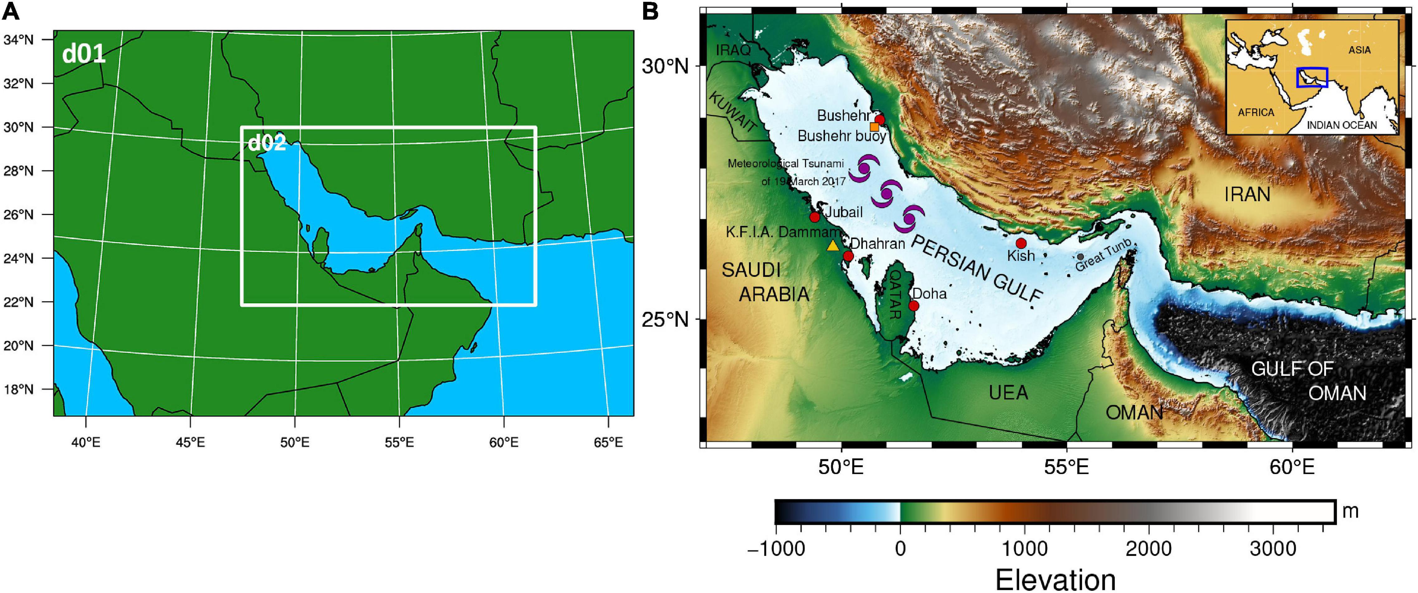
Figure 1. (A) Weather Research and Forecasting (WRF) domain setup D01 and D02. (B) Topographic map of the Persian Gulf and Gulf of Oman and locations of synoptic stations (red circle), wave buoys (dark orange rectangle), and radiosonde station (yellow triangle). The Topography data were derived from the SRTM15 + V2.0 at 15-arc sec resolution.

Meteotsunami are shallow-water waves or water level fluctuations due to atmospheric interactions, which typically last from minutes to hours (Monserrat et al., 2006). The development of these long waves depends upon several factors and has a multi-stage process; but meteotsunami generally begin with a sudden change in air pressure and/or wind (the effect of atmospheric turbulence) and are usually accompanied by mesoscale systems such as frontal passages, storms and strong winds (squalls), thunderstorms and gravitational waves of the atmosphere (Monserrat et al., 2006; Shi et al., 2020). The occurrence of meteotsunami long waves, especially when followed by high energetic wind-induced waves cause severe damage to the coastal environment, destroy infrastructure, and are potentially considered a large threat for local people since they are generally unexpected (Rabinovich, 2020).

Concerning the nature of the meteotsunami phenomenon, simulation of meteotsunami requires a high-resolution atmospheric model to provide a precise estimation of wind stress and pressure disturbances at the sea level (Shi et al., 2019). In addition, having an unembellished atmospheric model is critical in the accurate simulation of meteotsunami waves (Horvath et al., 2018; Shi et al., 2019) which depends on various factors such as grid resolution, physics, initial conditions, and selected boundaries in the simulation (Borge et al., 2008). Considering the non-linear and turbulent nature of the atmosphere, small differences in initial condition or model parameters lead to different representations of perturbations (Shi et al., 2019, 2020; Mourre et al., 2021). A common approach to deal with these sensitivities and forecast uncertainties in numerical weather models is to use an ensemble prediction (Borge et al., 2008; Horvath and Vilibić, 2014; Mourre et al., 2021). Horvath and Vilibić (2014) in their study on meteotsunami Boothbay, examined the sensitivity of high-resolution weather conditions and its relationship with model parameters, time step, initial and boundary conditions, and nested strategy. Belušić et al. (2007) studied meteotsunami events in the Adriatic Sea in 2003 and found that the wave-convection system is very sensitive to the microphysics used in the model. Mourre et al. (2021) evaluated different physical parameterizations in the implementation of a high-resolution atmospheric-ocean model with a nested network to predict a meteotsunami that occurred in Ciutadella (Spain). The results indicate the success of the extensive expansion of ensemble simulations regarding the prediction of the ultimate magnitude of meteotsunami. However, the small-scale characteristics of these disturbances were highly sensitive to the tuning parameters, which led to significant differences in the magnitude of the simulated response at sea level.

This study aims to assess the performance of different parameterizations for physical processes in a high-resolution numerical model in simulating the meteorological characteristics and wind-induced waves during the dominance of meteotsunami in the Persian Gulf. These simulations were carried out using Weather Research and Forecasting (WRF) model to determine the atmospheric parameters, and WAVEWATCH-III model to determine the wave spectrum. The wind and wave regimes of the Persian Gulf for a 31-yearly period were evaluated by Kamranzad (2018). The results indicated that monthly mean and extreme wave height for Bushehr station in March were lower than.6 m and higher than 3 m, respectively. As will be shown in section “Skill Assessment of WAVEWATCH-III,” the recorded wave height exceeds 1.5 m during the dominance of the meteotsunami (19–20 March); hence, the skill assessment of the WAVEWATHC-III model using different wind data is another goal of the study. The weather stations and buoy measurements were used for the models’ assessment. The study area, modeling system, and experimental approach are described in section “Materials and Methods”. Section “Results” includes the skill assessment of models, followed by conclusions in section “Conclusion.”

Materials and Methods

Study Area and Observations

The Persian Gulf is a semi-closed marginal sea on a continental shelf extended in a northwest-southeast direction and is located within the 24–30°N latitude and 47–52°E longitude, respectively (see Figure 1). The average depth of this water body is 37 m and it has access to the Gulf of Oman as well as the Indian Ocean through the Strait of Hormuz. The length of the Persian Gulf is approximately 1,000 km, its maximum width is 336 km and its maximum depth is approximately 90 meters near the Great Tunb Island; Also, the west and south side of the Persian Gulf is relatively shallow and has mild slopes (Reynolds, 1993). The Strait of Hormuz restricts the interaction of the Persian Gulf with open oceans (Liao and Kaihatu, 2016). Nayak et al. (2016) showed that the waves formed in the Gulf of Oman have negligible effects on the evolution of waves in the Persian Gulf due to energy loss during their crossing the Strait of Hormuz.

Mixed tides with a height of 1 to 2 m dominate most of the Persian Gulf (Akbari et al., 2016). The climate of the Persian Gulf is divided into two important seasons and two transitional periods. The summer season happens from May to September. In contrast, the winter season starts in November and finishes in March (Athar and Ammar, 2016). The winds are mainly from the northwest throughout the year. In winters, between November and February, wind speeds (mean value ∼5 m/s) are stronger than in summer (mean value ∼3 m/s) (Thoppil and Hogan, 2010). The most famous climatic phenomenon in the Persian Gulf region is the north-northwest wind called Shamal wind. It is a monsoon, systematic, continuous, and strong wind in the Persian Gulf. In summer, it blows mainly between May and July while in winter, it occurs between December and early March. However, this phenomenon is often not accompanied by coastal floods and generally causes waves between 0.25 to 0.4 meters in the northernmost coastal areas of the Persian Gulf (Thoppil and Hogan, 2010; Kazeminezhad et al., 2021).

The meteotsunami on 19 March 2017 occurred during a calm and cloudy day (Heidarzadeh et al., 2020). At 8:00 AM (+ 4:30 GMT), large long waves affected an area of about 100 km on the northern coasts of the Persian Gulf and caused more than 1 km of inundation in coastal and urban zones of Dayyer and Kangan. Pieces of evidence and field studies show that the height of the forerunner low-frequency wave exceeded 3 m near the port of Dayyer and has caused extensive damages in terms of life and economy in this region (Salaree et al., 2018).

Atmospheric systems generally produce meteotsunami with a spatial scale of hundreds of kilometers and a time scale of several hours, which is called mesoscale systems. Because small disturbances of atmospheric pressure (less than 1 hPa) and wind speed changes (10 m/s) in mesoscale systems usually cause disturbances at sea level on a scale of several centimeters, reinforcement mechanisms are required for large meteotsunami. Wave velocity in shallow water is highly dependent on water depth. Most meteotsunamis are reported to occur in semi-enclosed environments such as gulfs, which indicates the importance of the shape and geometry of the region (Williams, 2020). Appropriate bathymetry condition (water depth less than 100 m) and appropriate mesoscale atmospheric phenomenon [e.g., fronts reported by Heidarzadeh et al. (2020)] led to the 2017 meteotsunami event in the Persian Gulf.

The data from several synoptic stations and one radiosonde station were used to validate the simulation results in the period of 15–23 March 2017. Surface data were obtained from 5 airport synoptic stations via Hourly Global Surface (DS3505) datasets of the National Climatic Data Center (NCDC). Also, hourly data from Bushehr wave recorder buoy were provided by the Port and Maritime Organization of Iran¹. Upper air atmospheric station data from the radiosonde data archive of NOAA-ESRL database were available from the King Fahd International Airport (K.F.I.A.-Dammam) WMO station code 40417, which were retrieved from the Wyoming radiosonde database². All these stations are shown in Figure 1B. Among many parameters recorded at synoptic stations, wind speed and air pressure are more important for a meteotsunami study (Šepić et al., 2015; Vilibić et al., 2016; Horvath et al., 2018; Shi et al., 2019, 2020).

In addition to these ground meteorological data, hourly ERA5 reanalysis data were available via³. This dataset has been produced by the European Center for Middle-range Weather Forecast (ECMWF) with a 31-km resolution over the Persian Gulf. The variations in air pressure measured at different stations were compared to the ERA5 data during the period 15–23 March 2017 in Figure 2.

FIGURE 2

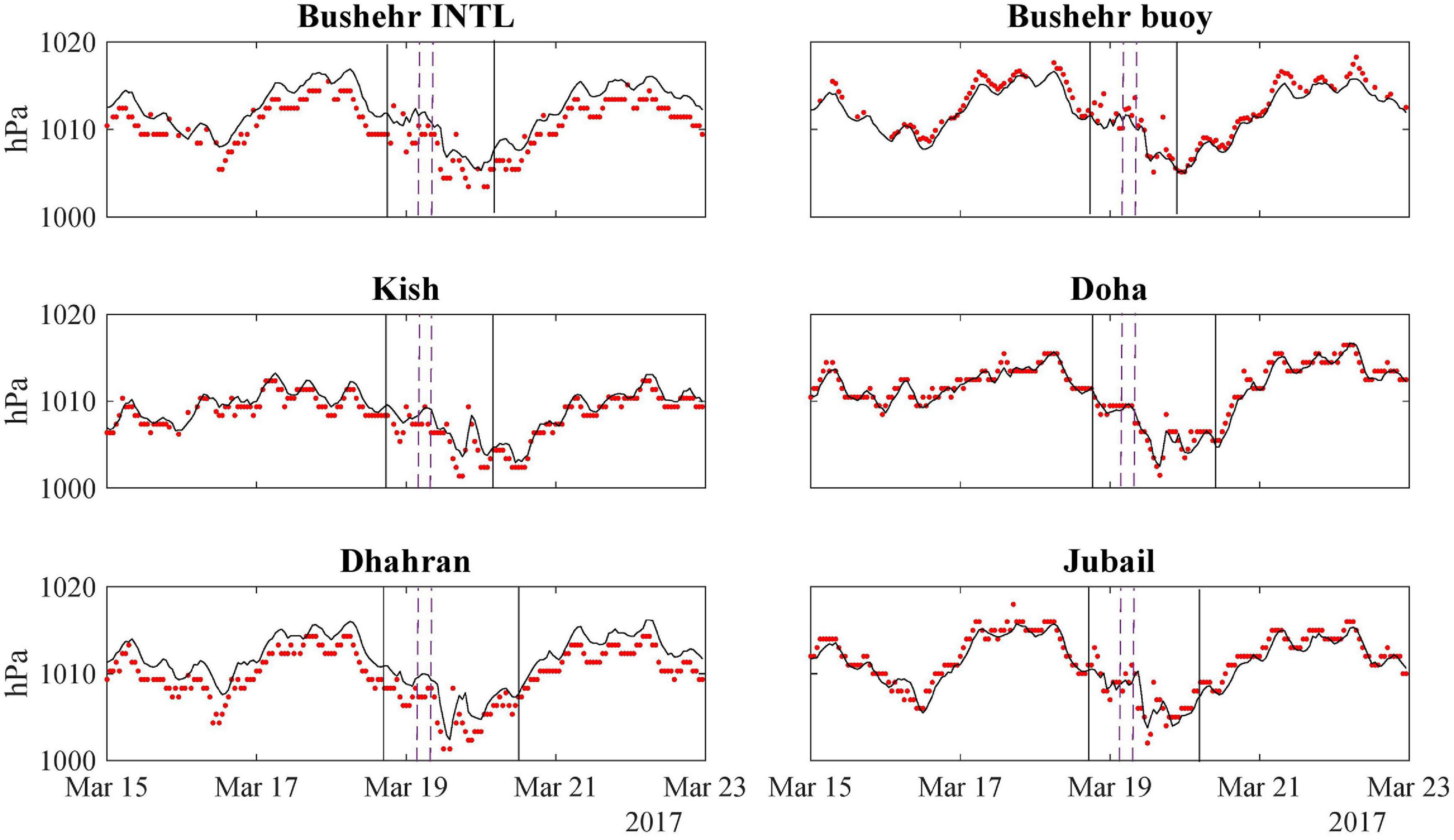
Figure 2. Atmospheric air pressure records during 15–23 March 2017, at the Persian Gulf coastal stations. The red dotted lines denote measured data from synoptic and buoy station and the black continuous line denote ERA5 data. The black lines denote distinct air pressure disturbances and the purple dashed line indicates the time of the Persian Gulf meteotsunami.

Fluctuations of atmospheric pressure on 19 March are following the period in which meteotsunami has occurred. Recorded pressure changes at Bushehr (synoptic and buoy) stations, Kish (synoptic and buoy), Daharan, Doha, and Jubail on 15–23 March 2017 are shown in Figure 2. Average air pressure begins to decrease at the end of 18 March 2017 and reaches its minimum value in the middle of 19 March in the shown period. At northern stations of the Persian Gulf, such as Bushehr and Kish, air pressure changes sharply and decreases by 4–8 hPa a few hours after the collision of tsunami-like waves (6:00 UTC). At Jubail and Daharan stations located in the southern part of the Persian Gulf, ∼2 hPa decrease in air pressure occurred last hours of 18 March followed by another drop in a range of 4 hPa, early morning on 19 March. It indicates that the low-pressure front was moving from the southwest of the Persian Gulf to its northeast part. The synoptic conditions of the Persian Gulf region and its areas at 4:00 and 6:00 AM on 19 March 2017 are shown in Figure 3 when tsunami-like waves were formed and hit the northern coasts of the Persian Gulf. Parameters such as average sea level pressure, the 10 m wind vectors, and wind gusts were obtained from the reanalysis dataset of ERA5. Since the cyclone was located in the northwest of the Persian Gulf at this moment, ERA5 data show the northeast wind direction over the Persian Gulf; i.e., in the opposite direction to the waves reaching the northern coasts of the Persian Gulf. The wind direction has been evaluated at Bushehr and Kish stations and the same pattern was observed. Thus, the ERA5 results were of good quality during this event based on stations located in the northern part of the Persian Gulf (both synoptic station and buoy of Bushehr). No strong gust wind was observed at these hours over the Persian Gulf; hence it is more likely that long waves during this meteotsunami phenomenon were created by atmospheric pressure fluctuations, which was in accordance with previous studies (Heidarzadeh et al., 2020; Kazeminezhad et al., 2021).

FIGURE 3

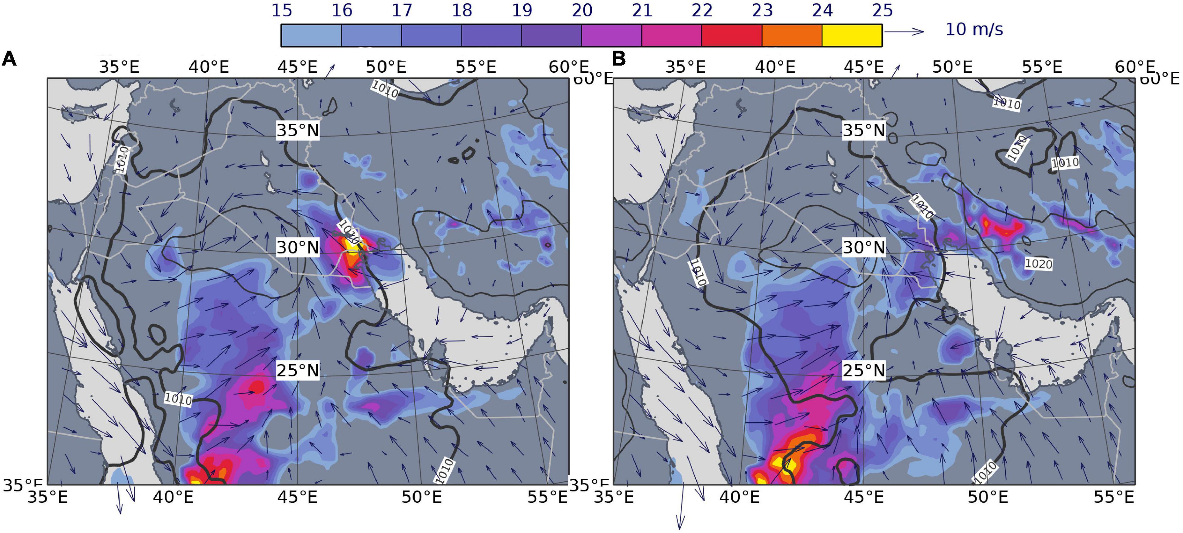
Figure 3. Mean sea level pressure contours, wind vectors at 10 m, and wind gust (shown by colors) at (A) 4:00 AM UTC; (B) 6:00 AM UTC.

Modeling System

The wind and wave simulations were performed as explained in this section.

Wind Model

In this study, the fully compressible, non-hydrostatic mesoscale Advanced Research WRF (ARW) version 4.3⁴ (Skamarock et al., 2019) is used on a Lambert conformal projection during 15–23 March 2017. It uses the Arakawa-C grid and a terrain-following hybrid sigma–pressure coordinate in the vertical direction for solving the governing equations. Runge–Kutta scheme is also utilized for the discretization in time-space. The model incorporates several parameterization schemes for physical processes including microphysics, cumulus convection, planetary boundary layer, land surface, and short and longwave radiations. In this study, WRF is configured with two nested domains with a horizontal grid spacing of 9 km (D01) and 3 km (D02), with 231 × 220 and 502 × 304 grid points (see Figure 1A). The domain center was located on the Kish Island. The vertical structure in both domains consists of 45 vertical levels from the sea surface to 50 hPa with varying vertical resolution such that, grid sizes are smaller near the ground and become coarser with increasing altitude.

High-quality initial and boundary conditions are crucial to have accurate simulations. These data were derived from the ECMWF IFS CY41r2 High-Resolution Operational Forecasts dataset⁵, which has 0.08° spatial and 6-h temporal resolution. The time step of the model simulation was set as 27 s in D01 and as 9 s in D02. The WRF Preprocessing System (WPS) in version 4.0.3⁶ was used to prepare the input data for the model together with the WPS V4 Geographical Static Data. To improve the accuracy of geographical data in the model, the modified IGBP 21-category, 15 arc-seconds, MODIS LULC database was adopted. The domain size and computational period were selected according to Heidarzadeh et al. (2020). The model was initialized at 6:00 PM on 14 March 2017, and the first 6 h of the simulation were taken as spin-up time.

Although the wind field of atmospheric models has high quality on the oceans and offshore areas, their performance in semi-closed and closed areas with complex geomorphology still needs improvements. The wind speed from a model in such conditions is less than observations in many cases (Cavaleri and Bertotti, 2003, 2006). Factors such as the position and size of the simulation domain, spatial resolution, and initial conditions affect the model results. In addition to selecting the appropriate dynamic configuration, testing and selecting the appropriate physical parameterization also reduce the uncertainties of atmospheric models in calculating the wind field (Belušić et al., 2007; Vilibić et al., 2008, 2016; Šepić et al., 2009; Horvath and Vilibić, 2014; Horvath et al., 2018; Linares et al., 2019; Shi et al., 2019, 2020; Mourre et al., 2021). There are many physical designs in the WRF model which make it flexible for different climatic conditions with optimal performance for a range of temporal and spatial resolutions (Skamarock et al., 2019).

A subset of physical parameterization including the planetary boundary layer (PBL), cumulus (CU), and the microphysics (MP), which has been used in previous meteotsunami studies, were used to optimize the model performance (Belušić et al., 2007; Šepić et al., 2009; Renault et al., 2011; Horvath and Vilibić, 2014; Horvath et al., 2018; Denamiel et al., 2019; Shi et al., 2019; Mourre et al., 2021). To be more specific, the following schemes have been used; (MP): the Thompson 6-class graupel scheme (Thompson et al., 2008) and the WSM6-class scheme (Hong and Lim, 2006); (CU): the Grell–Devenyi ensemble scheme (Grell and Dévényi, 2002), the New Tiedtke Scheme (Zhang and Wang, 2017) and the Kain–Fritsch scheme (Kain, 2004); (PBL): the Yonsei University scheme (Hong et al., 2006), the Mellor-Yamada-Janjic (MYJ) scheme (Janjić, 1994) and the Mellor-Yamada-Nakanishi-Niino (MYNN) 2.5 scheme (Nakanishi and Niino, 2006). The YSU PBL scheme was used along with the revised MM5 similarity theory surface layer (Jiménez et al., 2012), while the MYJ and MYNN PBL scheme was used along with the Eta similarity scheme (Monin and Obukhov, 1954) and MYNN scheme (Nakanishi and Niino, 2006) respectively. For all simulations, the Noah–MP (Niu et al., 2011) land surface scheme was used. The Goddard scheme for shortwave (Chou and Suarez, 1994) and the Rapid Radiative Transfer Model [RRTM; Mlawer et al. (1997)] for longwave radiation was used. Since domain resolution was less than 5 km, the cumulus parameterization was switched off for the local domain in all simulations according to Athukorala et al. (2021). The parameterization schemes incorporated into the model are summarized in Table 1.

TABLE 1

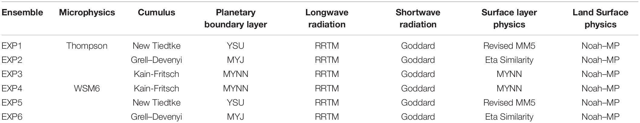
Table 1. List of the physical options for WRF modeling.

Wave Model

The WAVEWATCH-III (hereinafter WWIII) is a state-of-the-art, phase-averaged model which numerically solves the conservation of wave action as below:

$\frac{dN}{dt}=\frac{S_{tot}}{\mathrm{\sigma }}(1)$

The left-hand side of Eq. (1) includes the local rate of change in wave action, wave propagation in x and y dimensions, and wave propagation in σ and θ spaces. The wave action N is equal to $\frac{E}{\mathrm{\sigma }}$, where E is wave energy density and σ is the angular frequency. The term S_tot incorporates a sink and source terms among which the exponential wind-wave growth (S_in), non-linear quadruplet (S_nl), and dissipation due to white capping (S_ds) are important in deep waters (WAVEWATCH III Development Group WW3DG, 2016).

Several packages are available for S_in and S_ds in WWIII. Janssen (1991) parameterized wind input term as a function of $\frac{u_{*}}{C}$, wave-supported stress, and wind logarithmic profile; where u_* is friction velocity and C is phase speed velocity, respectively. This method needs an iterative process to obtain u_* which is valid simultaneously in both wave-supported stress and wind profile. This method is known as WAM-Cycle4 or ST3 formulation in WWIII.

The whitecap dissipation in ST3 includes weighted linear and non-linear dependency to wave numbers using δ₁ and δ₂ = 1 − δ₁ coefficients. The C_ds is a tuning parameter in this formulation while $\overline{k}$, $\overline{\mathrm{\sigma }}$, $\overline{\mathrm{\alpha }}$ are mean wave number, mean angular frequency and mean steepness, respectively.

$S_{ds}(k,\mathrm{\theta })=C_{ds}\left({\overline{\mathrm{\alpha }}}^2\right)\overline{\mathrm{\sigma }}\left[{\mathrm{\delta }}_1\frac{k}{\overline{k}}+{\mathrm{\delta }}_2{\left(\frac{k}{\overline{k}}\right)}^2\right]N(k,\mathrm{\theta })(2)$

In this research δ₁ and C_ds will be considered as tuning parameters.

The most recent package for wind input and energy dissipation implemented in WWIII is ST6. The wind input term includes two parts that depend on wave direction (θ), wind direction (θ_w), wind velocity (U), and C. The w₁ part controls the wind input term when cos(θ−θ_w) is greater than 0; otherwise w₂ will be dominant which includes ‘negative wind input’ (Donelan et al., 2006).

$\begin{array}{c}{w}_1=ma{x}^2\{0,\frac{U}{C}\cos \left(\mathrm{\theta }-{\mathrm{\theta }}_w\right)-1\},\hfill \\ w_2=mi{n}^2\{0,\frac{U}{C}\cos \left(\mathrm{\theta }-{\mathrm{\theta }}_w\right)-1\}\hfill \end{array}(3)$

$w=w_1-a_0{w}_2(4)$

In this study, a₀ was set to 0.09 according to Liu et al. (2017). In Eq. (3), U could be scaled with 32u_* to avoid overestimation of energy levels at high frequencies (Liu et al., 2019). This scale was used in many recent research [e.g., Christakos et al. (2020), Kalourazi et al. (2020), Beyramzadeh et al. (2021)].

The whitecap dissipation in ST6 includes T₁ term which presents the inherent breaking term, and T₂ term which describes the cumulative effects of short-wave breaking due to longer waves [Rogers et al. (2012), Zieger et al. (2015)]:

$S_{ds}(k,\mathrm{\theta })=\left[T_1(k,\mathrm{\theta })+T_2(k,\mathrm{\theta })\right]N(k,\mathrm{\theta })(5)$

These T₁ and T₂ terms have tuning coefficients a₁ and a₂ which were used for calibration.

Wind vectors, bathymetry, and open boundary conditions are crucial for wave models. Besides six introduced wind experiments presented in Table 1, the original ERA5 wind data were used as wind input for wave simulations. The temporal resolution for all wind data was 1 hour. Both ST3 and ST6 formulations were used to reproduce H_s and T_p. Default values for tuning parameters in ST3 were C_ds = -4.5 and δ₁ = 0.5. For ST6 formulation, a₁ = 4.75×10⁻⁶ and a₂ = 7×10⁻⁵ were default values. These ST3 and ST6 formulations were calibrated against AD measurements and altimeter data using ERA5 wind in the Persian Gulf and the Gulf of Oman by Beyramzadeh et al. (2021) (hereafter BSD2021). Their suggested values for tuning parameters were also used which are C_ds = -1.5 and δ₁ = 0 for ST3, and a₁ = 1.05 ×10⁻⁷ and a₂ = 1.74 ×10⁻⁶ for ST6. Therefore, ERA5 wind data will be assessed using two sets of coefficients: (1) described default tuning values for ST3 and ST6 formulations (2) suggested calibration values by BSD2021 for the Persian Gulf.

The bathymetry data were extracted from The General Bathymetric Chart of the Oceans (GEBCO) which were released with high spatial resolution 0.004° in 2019. Hourly boundary conditions were extracted in the form of directional wave spectra from a global wave modeling. Directional wave spectra were implemented along the southern (23°N, 59.2°−61°E) and eastern (61°E, 23°−25.2°N) open boundaries of the computational domain. More details about the global model were presented in BSD2021.

The computational grid in the WWIII model covers 47.2°−61°E and 23°−31°N using a rectangular grid with 0.04°×0.04° resolution. Following Siadatmousavi et al. (2012), 30 frequencies with geometrical distribution were considered in the range of 0.04–0.63 Hz. Moreover, 36 directions with 10° resolution were applied. Four time-steps are needed in the WWIII model: (1) maximum global time-step was set as 360 s; (2) the maximum CFL time-step for x-y was set as 180 s; (3) the maximum CFL time-step for k-theta was set as 360 s; (4) time-step for source term was set as 30 s.

The non-linear quadruplet wave-wave interaction (S_nl) mainly controls wave spectrum evolution in wave models. It is the most time-consuming term in simulations; therefore, the DIA (Discrete interaction Approximation) method proposed by Hasselmann et al. (1985) has been presented for operational applications. Resio and Perrie (2008) and Perrie et al. (2013) compared the obtained S_nl term for the JONSWAP spectrum with different peak enhancement parameters (γ = 1, 3.3, and 7) against the exact solution (Webb-Resio-Tracy method). For fully developed spectrum (γ = 1), the positions of positive and negative lobes are identical with the exact solution, but the DIA overestimates (underestimates) positive (negative) lobes. As a consequence, more dissipation and more wind input energy are needed on forward and rear faces, respectively. Simulated S_nl term with the DIA deviates from the exact solution with increasing γ parameter. Furthermore, spurious positive and negative lobes have appeared on the rear face of the spectrum. It is inferable that the deficiencies of the DIA method in reproducing S_nl the term should be compensated with other sink and source terms (S_in and S_ds). It is expected that the wind input and whitecap calibration with the DIA method might result in unrealistic coefficient values.

The Gaussian Quadrature Method (GQM) is a recent method to estimate S_nl term in deep water conditions, developed by Lavrenov (2001) and implemented as a portable Fortran module in the TOMWAC model by Benoit (2005). The GQM method strongly depends on the integration resolution. Rough, medium, and fine resolutions were evaluated in duration and fetch limited test cases, slanting fetch, and test cases with varying wind direction. More agreement with the exact solution is expected when medium and fine resolutions were applied, while they are more expensive than rough resolution and the DIA method (Benoit, 2005, 2007; Gagnaire-Renou et al., 2009; Gagnaire-Renou et al., 2010). For the first time, the GQM with the medium resolution was implemented in the WWIII model and used to simulate wind waves during the presence of meteotsunami in the Persian Gulf. Similar to the DIA, this method was combined with a depth scale proposed by Komen et al. (1994) to be used in the shallow water of the Persian Gulf.

Statistical Indices

For this part, three statistical indices were applied to skill assess the WRF and WWIII models against measurements: mean bias error (MBE), root mean square error (RMSE), and index of agreement (d) presented by Willmott (1982):

$MBE=\frac{\sum (M_i-O_i)}{N}(6)$

$RMSE=\sqrt{\frac{1}{N}\sum {(M_i-O_i)}^2}(7)$

$d=1-\frac{{(M_i-O_i)}^2}{\sum {(\left|M_i-\overline{O}\right|+\left|O_i-\overline{O}\right|)}^2}(8)$

in which M_i and O_i are modeled and observed data, respectively. N is the total number of observations. All indicators are calculated with hourly data. Note that d is a dimensionless index that quantifies the agreement between the two series of data; the value of d index larger than.5 indicates good performance of the model.

Results

Skill Assessment of Weather and Research Forecasting Model

Taylor diagram and statistical parameters (MBE) for different stations and different experiments are designated in Figures 4, 5. Also, the value of the agreement coefficient parameter (d) for each station is given in Table 2. Taylor diagram is a statistical summary that presents the correlation coefficient, normalized standard deviation and root mean square error (Taylor, 2001). As seen from Figure 4, EXP1 and EXP2 were superior to other experiments at Bushehr and Kish stations for predicting wind pressure and speed. The agreement index and the correlation for wind speed for all experiments at Bushehr station were more than 0.6, indicating that all of them had acceptable performance according to Borge et al. (2008). The correlation coefficients between wind speed data from observations and simulations at Kish station were less than.5. At Bushehr buoy station, EXP4 had good performance for pressure, and EXP2 and EXP4 had good performance for wind speed. The MBE values of surface air pressure at Bushehr synoptic station, Bushehr buoy, and Kish station indicate that pressure values are generally overestimated. No trend exists for wind speed; e.g., the wind speed at Bushehr synoptic station is underestimated while it is overestimated at Bushehr buoy station. At Kish station, unlike other experiments, the MBE values for EXP3 and EXP4 were negative. The MBE value for EXP2 at this station was close to zero. In general, according to Figure 4 and Table 2, at northern Gulf stations, EXP3 and EXP4 (using Mellor-Yamada-Nakanishi-Niino scheme for planetary boundary layer and surface layer) slightly overestimated the surface pressure at the ground level stations and underestimated the wind speed. In contrast, over the water body (i.e., at Bushehr buoy), they tend to reduce the amount of surface pressure and relatively increase the wind speed compared to other schemes.

FIGURE 4

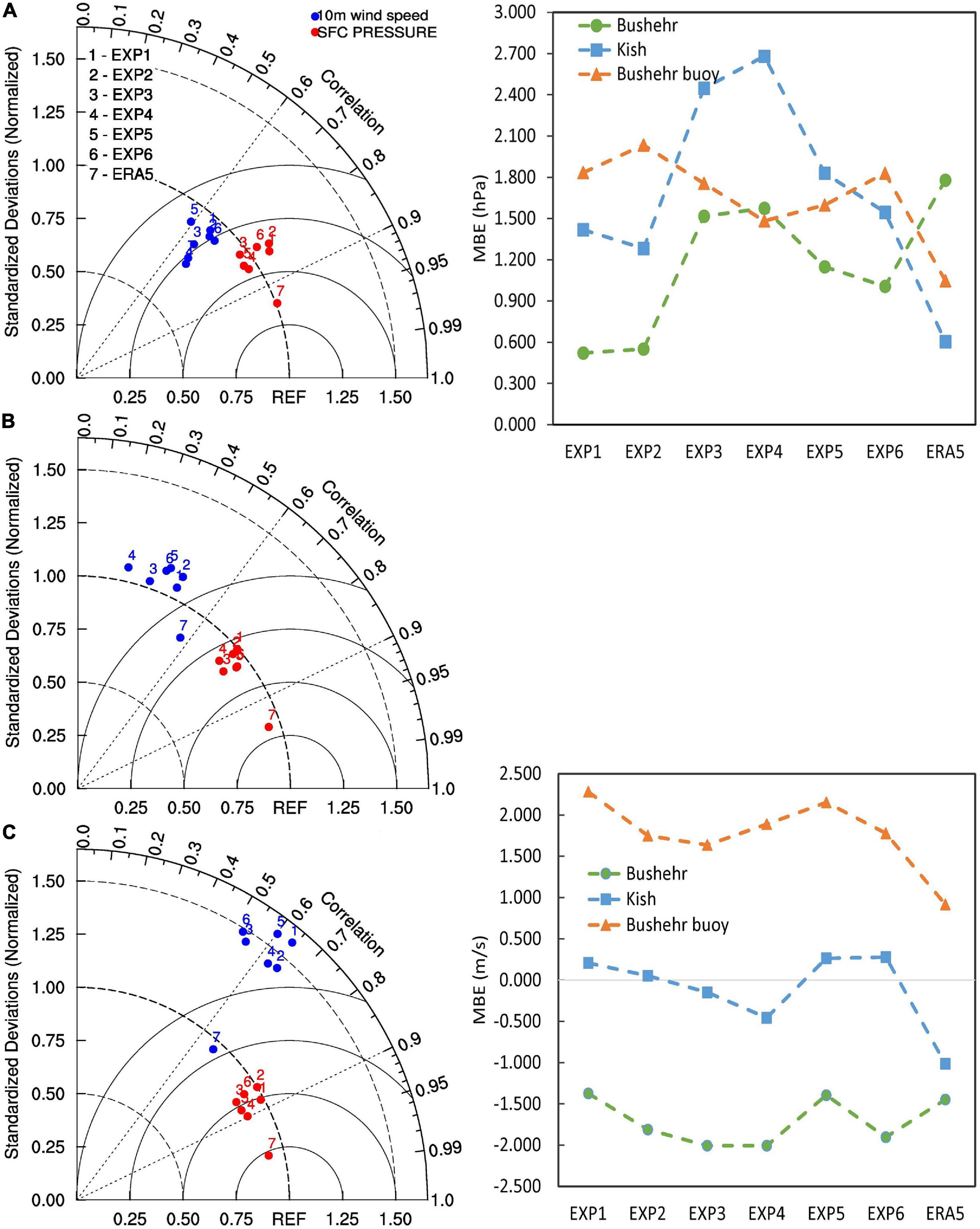
Figure 4. Taylor diagram of surface air pressure and wind speed at (A) Bushehr INTL, (B) Kish, and (C) Bushehr buoy for six WRF experiments and ERA5 data. Right charts show mean bias error for pressure and wind speed. Standard deviation and RMSE are normalized by the standard deviation of observations at the relevant temporal frequency.

FIGURE 5

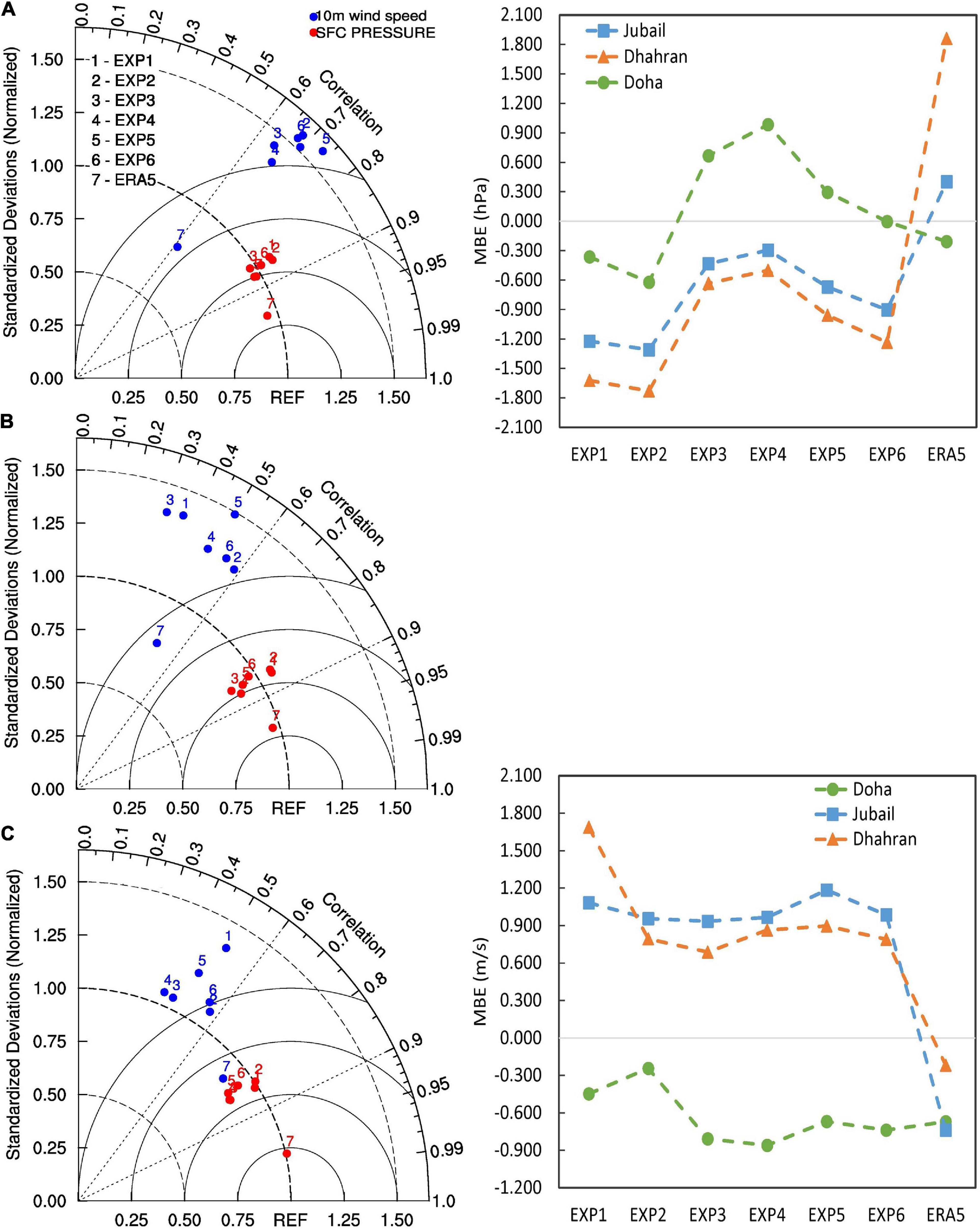
Figure 5. Taylor diagram of surface air pressure and wind speed at (A) Jubail, (B) Dhahran, and (C) Doha stations. Right charts show mean bias error for pressure and wind speed.

TABLE 2

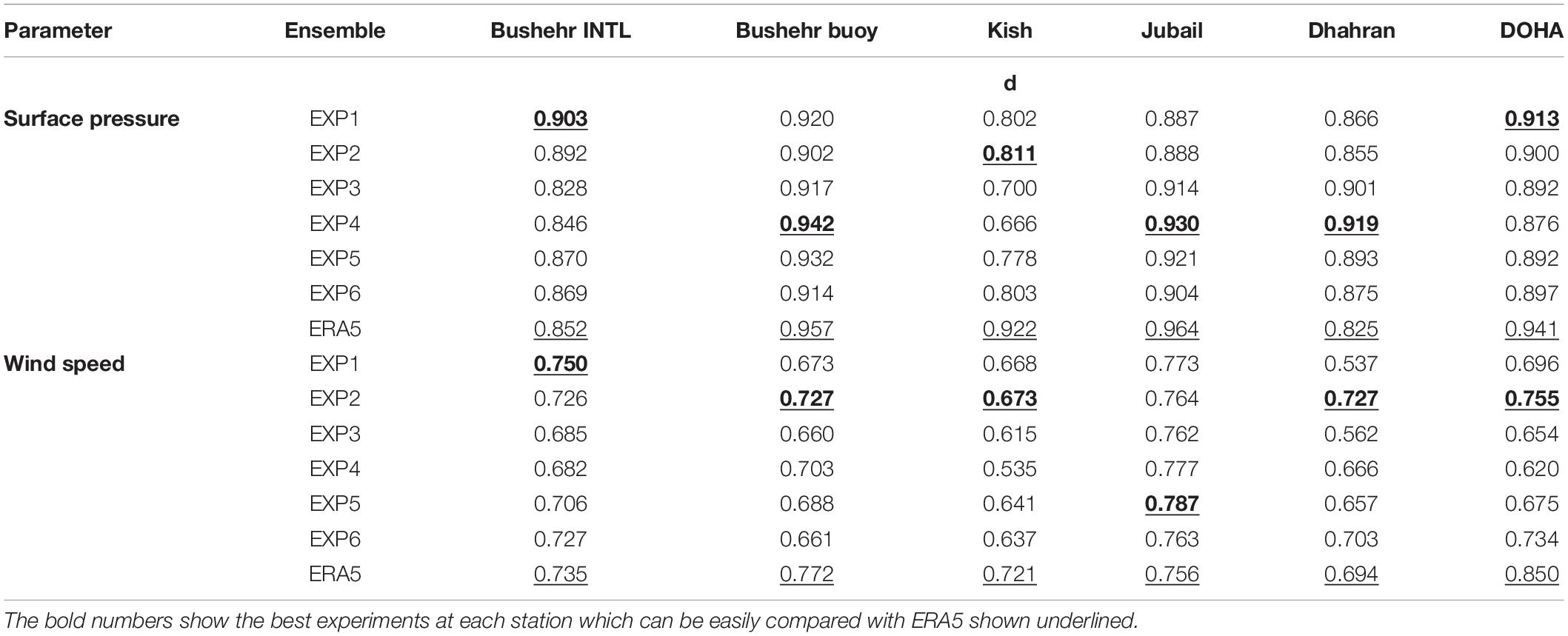
Table 2. Index of agreement (d) between model results and in situ observations at the different synoptic stations and wave buoys considered in the present study.

As shown in Figure 5, at Daharan, Jubail, and Doha stations, EXP2 and EXP4 configurations were more successful than other combinations for surface pressure and wind speed estimation, respectively. At these ground-level stations, the MYNN boundary layer scheme increased surface pressure and relatively decreased wind speed compared to YSU and MYJ schemes. The results of combining the MYNN planetary boundary layer scheme and the Thompson microphysics scheme were better than the MYNN and WSM6 microphysics scheme for pressure and wind speed estimation. Unlike stations of the northern Persian Gulf, at these stations (except the three ensembles No. 3, 4, and 5 at Doha station), the estimation of surface pressure was less than the observations. Wind speed was underestimated at Doha station and overestimated at Jubail and Daharan stations. In general, the MYJ boundary layer scheme, which is a local influenced scheme, resulted in a better estimation of wind speed than two non-local YSU and local MYNN schemas in the Persian Gulf meteotsunami occurrence period. Regarding the index of the agreement for pressure and wind speed obtained from different ensembles of the WRF model as well as ERA5 data, improvements at some stations were obtained using WRF model ensembles compared to ERA5 data.

The time series of pressure and wind speed from different WRF configurations and ERA5 data at two synoptic stations and Bushehr buoy are designated in Figure 6. The transverse of a low-pressure system has been resolved by all scenarios on 19 March and 20 March in all simulations.

FIGURE 6

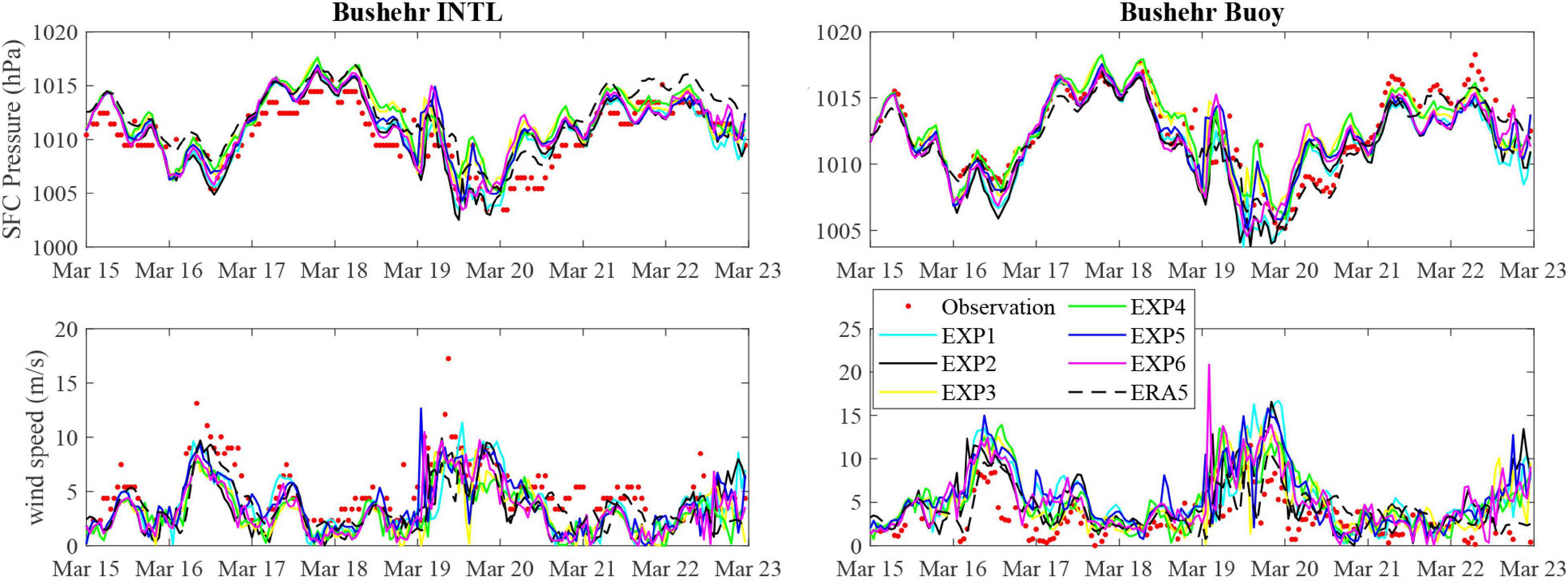
Figure 6. Time series of the observed (red dotted line) and model-predicted air pressure (hPa) and wind speed (colored solid line) at the Bushehr synoptic and buoy stations.

Regarding MBE at these two stations, which is also characterized in Figure 4, the predicted pressure values in all simulations were greater than the observations. The EXP4 had better estimates of pressure changes on the water surface than on land. Wind speed time-series changes also indicated that the overall trends of simulations were close to observations; however, all of them underestimated the wind speed during peaks (including meteotsunami occurrence) at the Bushehr synoptic station. The configurations EXP2 and EXP1 outperformed others in reproducing wind speed at this station. In contrast, all experiments overestimated the wind speed at the Bushehr buoy. The worst-case was EXP6 which predicted 20 m/s wind speed at the moment of meteotsunami occurrence.

The results of the WRF simulated and measured radio-sounding data at 12 UTC on 19 March 2017, are compared and presented in Figure 7. In general, all simulations accurately reproduced the temperature and moisture content of the atmosphere but overestimated the moisture content in the upper troposphere. Also, at pressure levels less than 250 hPa, the temperature value was overestimated in all simulations. The same occurred near the ground surface by EXP1 and EXP2 parametrizations. The temperature changes were smooth in EXP3. This configuration showed a sudden temperature inversion in the middle of 500–700 hPa pressure level; however, this configuration was not able to simulate temperature changes in the upper troposphere. EXP2 parameterization had a better ability to estimate moisture content in the atmosphere. The closeness of the dew point temperature to the air temperature at pressure levels of 300–700 hPa was well simulated by this parametrization. The maximum wind speed was observed at a pressure level of 250 hPa at the measuring station; however, it was estimated to occur close to 500 hPa in all simulations. In sum, the EXP2 configuration (using Mellor-Yamada-Janjic scheme for the planetary boundary layer, Grell–Devenyi cumulus scheme, and Thompson microphysics scheme) provided the most realistic results regarding atmospheric moisture content and vertical temperature parameter in the Persian Gulf during the period of meteotsunami event on 19 March 2017.

FIGURE 7

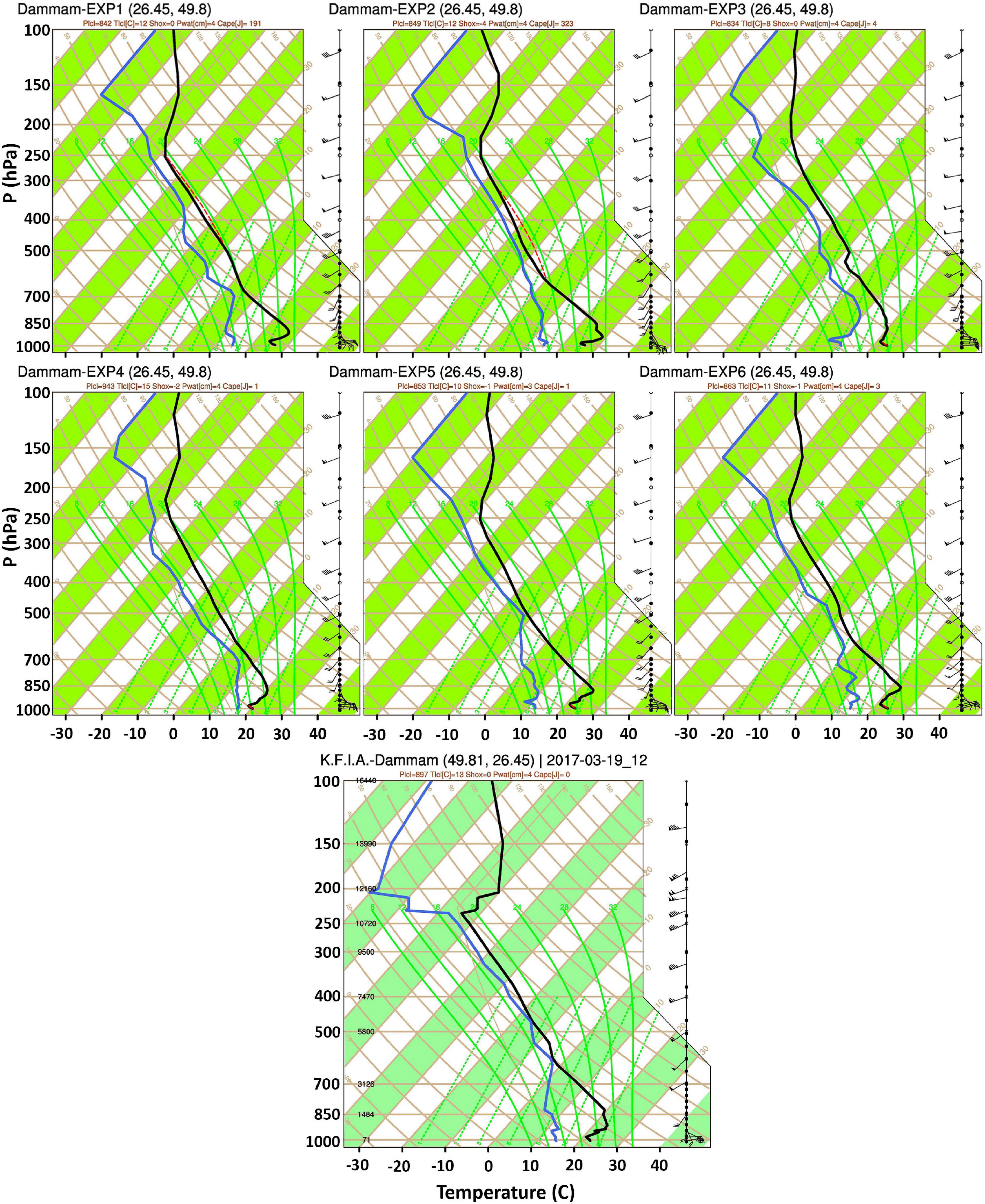
Figure 7. Skew-T diagrams from six different WRF parameterizations at 12 UTC 19 March 2017. The continuous black line represents temperature, and the continuous blue line represents dew point temperature variations along the vertical atmosphere.

The maximum radar reflectivity has been investigated to further evaluate the intensity and structure of convective clouds and assess the sensitivity of the mesoscale simulations to the choice of the microphysics and convective parameterization (see Figure 8). The results from the innermost model domain were used. Note that in both outermost and innermost domains, heat and moisture tendencies were determined by microphysics parameterization. Therefore, the effects of convective parameterization propagated from the outermost domain to the innermost domain. Model-derived maximum radar reflectivity at 4:00 AM 19 March 2017 showed that simulations with WSM6 microphysics produced slightly stronger reflectivity, especially in the southern part of the domain. Comparisons with radar data showed that in this area, both WSM6 and Thompson microphysics provided excessive reflectivity [cf. Figure 10 in Kazeminezhad et al. (2021)]. Also, simulations with the Kain–Fritch scheme provided too intense radar reflectivity. The overall shape of maximum reflectivity distribution at this moment was well simulated by EXP2 parametrizations.

FIGURE 8

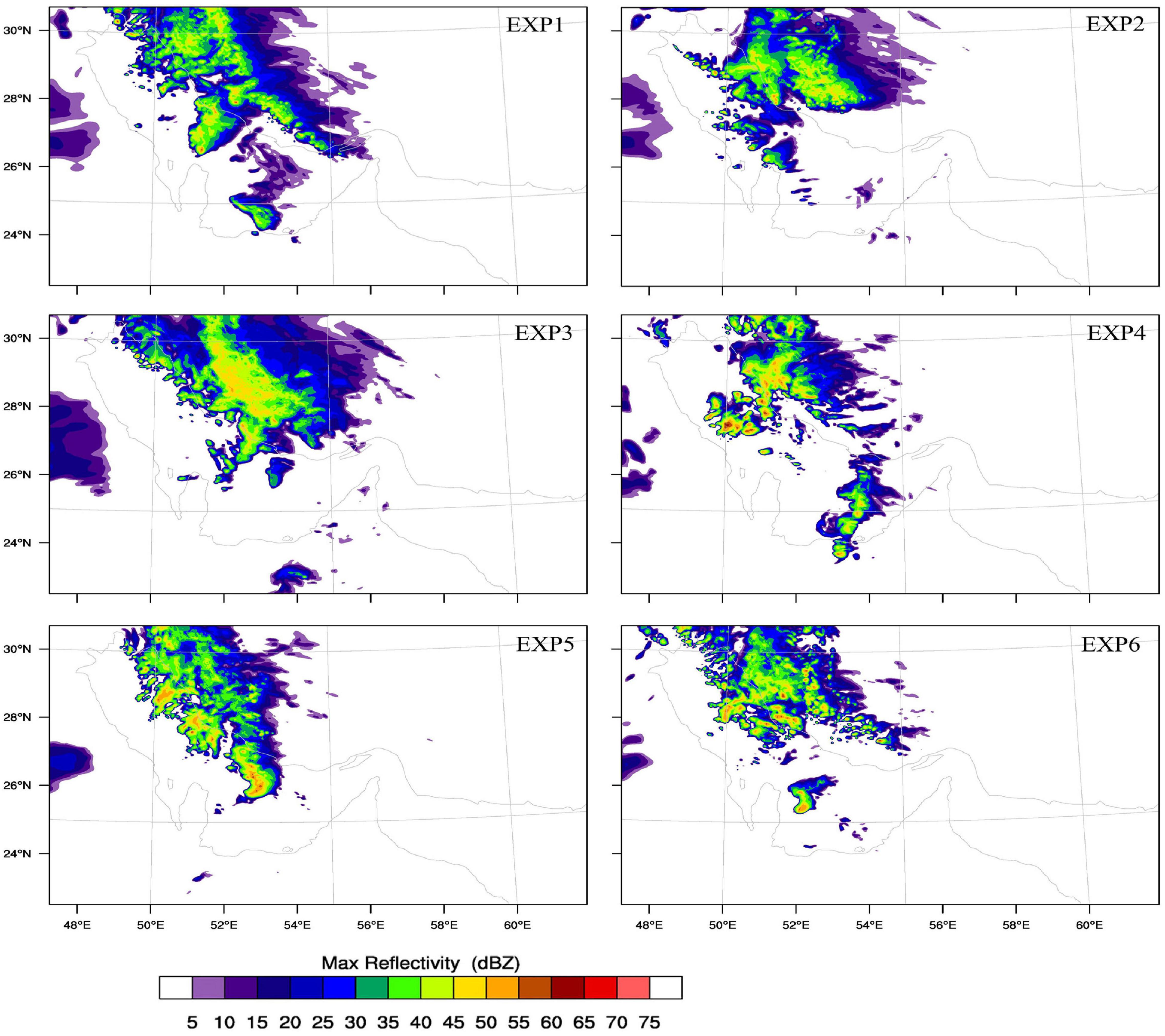
Figure 8. Simulated maximum radar reflectivity (mDBZ) at 4:00 AM 19 March 2017 for six different WRF parameterization.

The maximum reflectivity index greater than 60 dbz was introduced by Šepić and Rabinovich (2014) and Kazeminezhad et al. (2021) as a signature for convective cells which followed with meteotsunami formation in the domain; however, a lower value of 40 dbz was also considered as a meteotsunami source in the Gulf of Mexico (e.g., Shi et al., 2019). The hourly simulated maximum reflectivity index was presented in Figure 9 using EXP2 from 12:00 to 4:00 AM UTC 19 March. Two nearly horizontal and vertical convective systems were entered the Persian Gulf at 12:00 AM from west and south, respectively. As time passed, the southerly vertical system weakened and eventually disappeared, while the westerly horizontal system strengthened to 55–60 dbz and spatially extended from 1:00 to 02:00 AM. It slightly decreased at 3:00 AM UTC; however, increased to 55–60 dbz at 4:00 AMUTC again as it moved eastward. Described pattern for simulated maximum reflectivity from 12:00 to 4:00 AM is in agreement with Bushehr weather radar data described by Kazeminezhad et al. (2021).

FIGURE 9

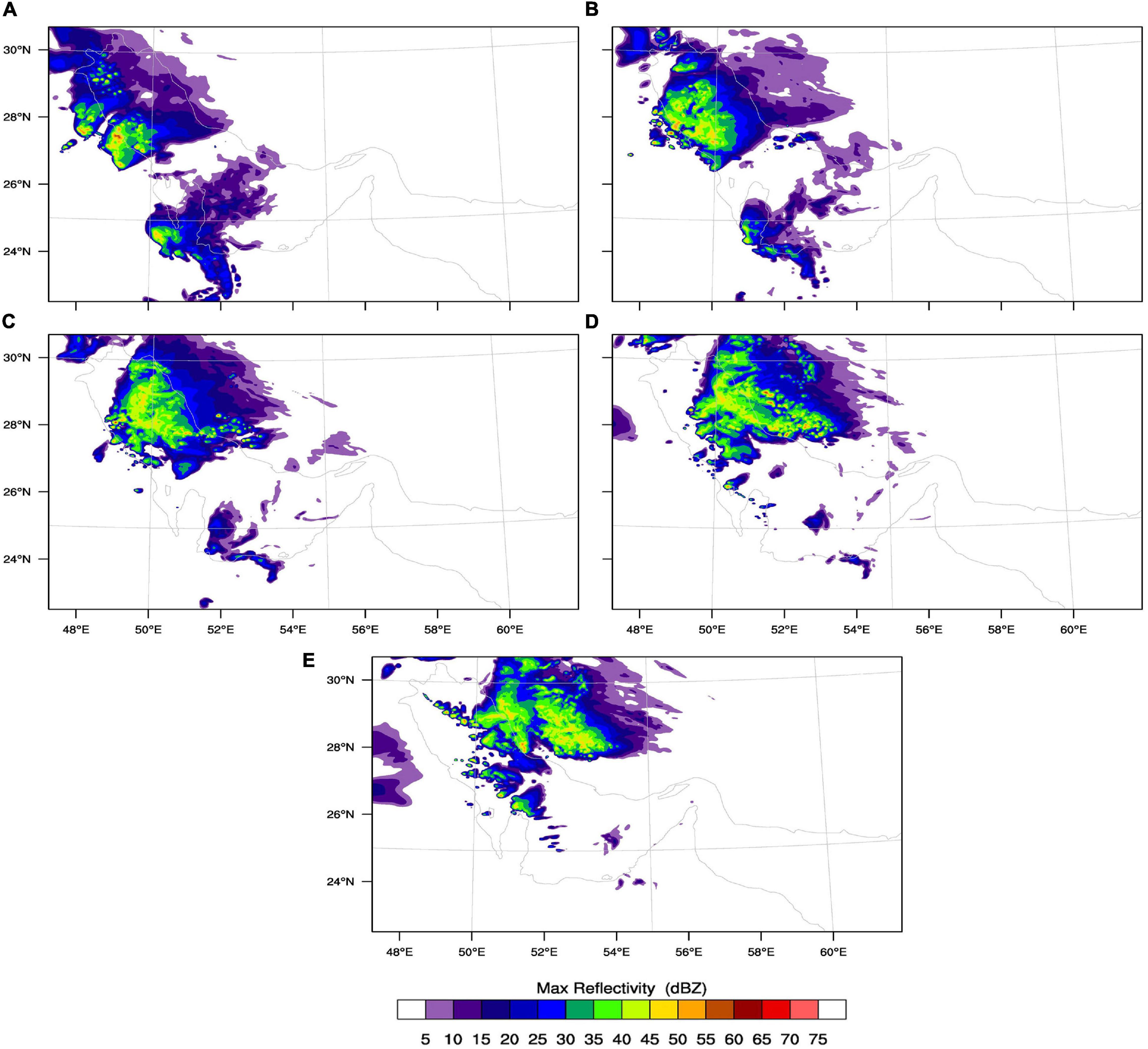
Figure 9. Simulated maximum radar reflectivity (mDBZ) using EXP2 configuration on 19 March 2017 at (A) 12:00 AM; (B) 1:00 AM; (C) 2:00 AM; (D) 3:00 AM; and (E) 4:00 AM.

Skill Assessment of WAVEWATCH-III

In Figure 10, Simulated H_s and T_p parameters with ST3 and ST6 packages of WWIII model for eight experiments were compared to buoy measurements at Bushehr during 15–23 March. The performance of the model using WRF experiments was close with small differences; e.g., EXP1 parameterizations resulted in the lowest absolute MBE and high RMSE for H_s hindcast. Also, EXP3 led to ∼0.1 H_s underestimation and low RMSE. Unlike H_s, EXP1 parameterization has severely underestimated T_p. The most successful configuration for reproducing T_p was EXP3.

FIGURE 10

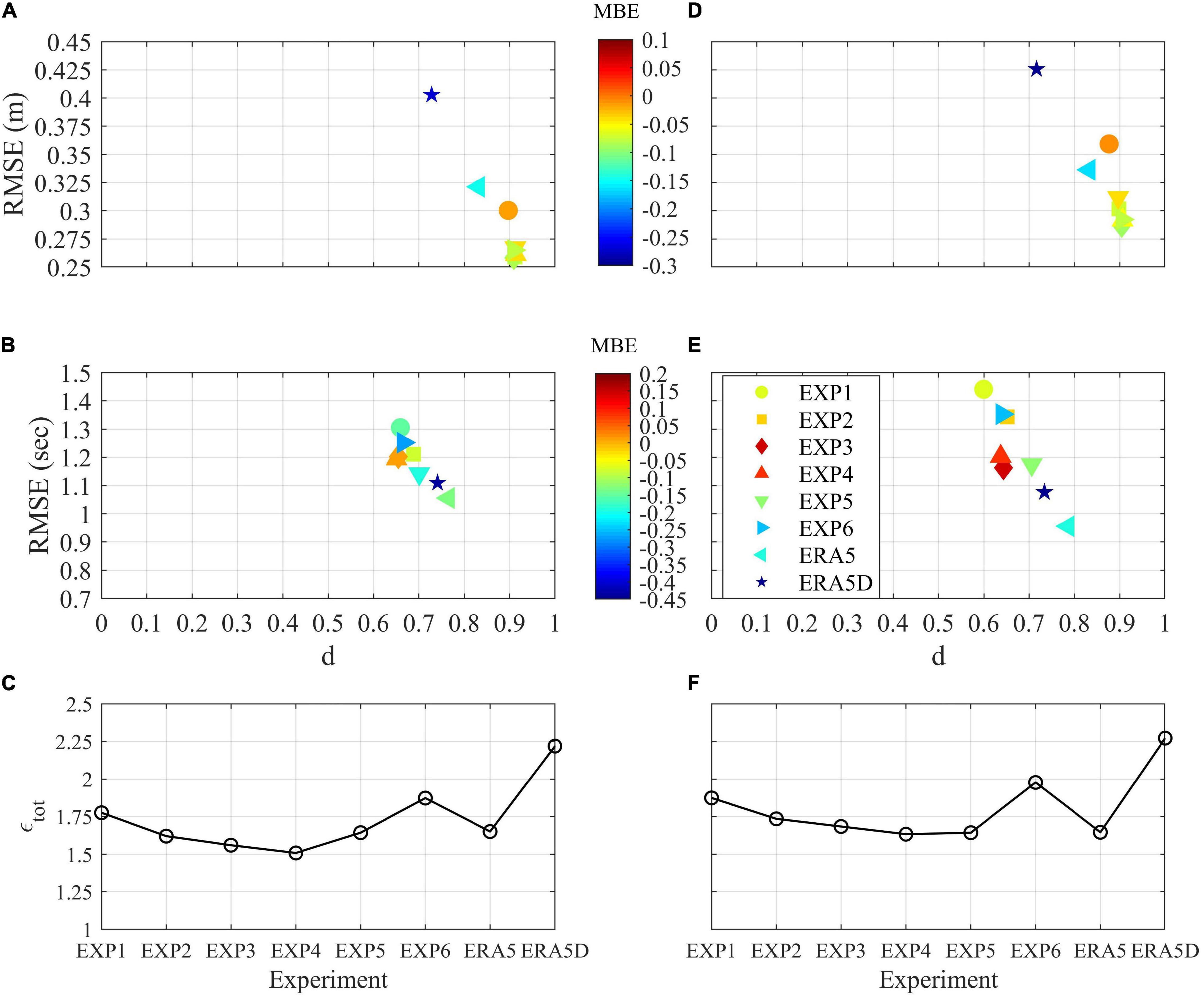
Figure 10. Simulated H_s and T_p compared with buoy measured data at Bushehr. The left and right panels are for ST3 and ST6 packages, respectively. (A,D) depict estimated MBE, RMSE, and d indices for H_s; (B,E) are the same as (A,D) but for T_p. (C,F) the ϵ_tot from Eq. (9).

Furthermore, ERA5 data with default coefficients of the model (ERA5D hereafter) severely underestimated H_s and T_p parameters. This experiment presented the worst performance in reproducing H_s. Unlike ERA5D, applying ERA5 wind data with the calibrated tuning values (ERA5 experiment) proposed for the Persian Gulf by BSD2021, considerably improved both H_s and T_p predictions. It is worth mentioning that the ST6 is more sensitive than ST3 to wind experiments. To determine the best configuration, the following error parameter _tot was defined:

${\mathrm{ϵ}}_{tot}={\left|MBE\right|}_{H_s}+RMS{E}_{H_s}+{\left|MBE\right|}_{T_p}+RMS{E}_{T_p}(9)$

This error parameter was evaluated for eight experiments and results are presented in Figures 10C,F. EXP4 parameterizations using ST3 resulted in the lowest _tot, while EXP4, EXP5 parameterizations and ERA5 experiments using ST6 could result in a similar low _tot value at Bushehr buoy; hence EXP4 at Bushehr station could be selected as the optimum configuration when either ST3 or ST6 was applied. ERA5D using both ST3 and ST6 packages led to high _tot which emphasized the importance of model calibration. The accuracy of ST3 was slightly better than ST6 at this station which is in accordance with BSD2021.

The time series of simulated and measured H_s, T_p and mean wave direction were presented in Figure 11. According to wind evaluations presented in Figure 10, EXP4 and ERA5 parameterizations were selected for further investigations using ST3 and ST6 formulations. As it is clear, H_s was underestimated by the ERA5 experiment at Bushehr buoy during events on 16–17 March and 19–20 March. In contrast, bulk wave parameters from EXP4 were in good agreement with the trend of measurements; hence, the ERA5 wind data was not suitable for wave hindcast during the dominance of meteotsunami in the Persian Gulf, while EXP4 parameterization led to reasonable performance when either ST3 or ST6 package was used with the default tuning values.

FIGURE 11

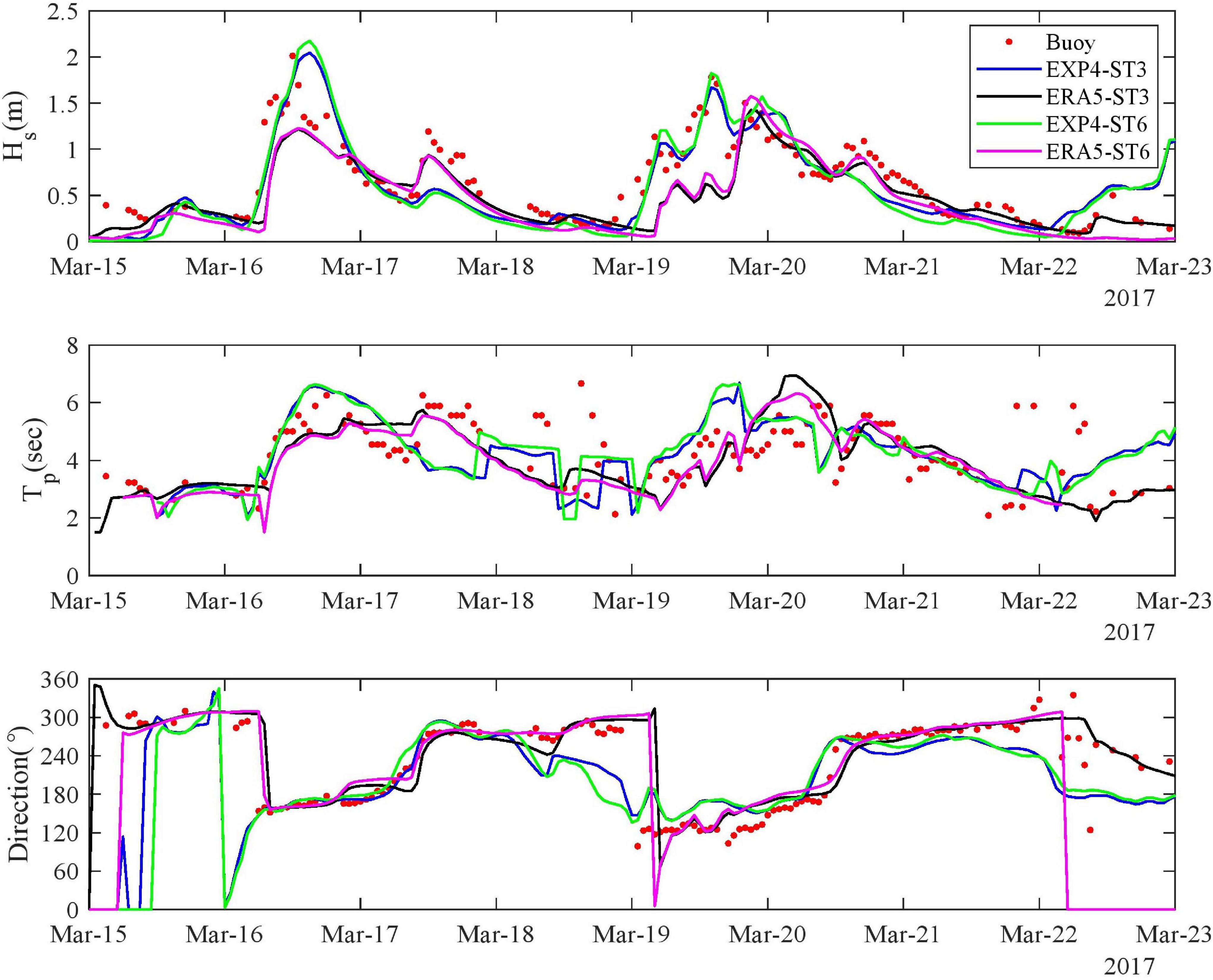
Figure 11. Time series of simulated bulk wave parameters and buoy data (red dots) at Bushehr using different configurations.

In Table 3, simulated H_s and T_p were used to assess the importance of S_nl term in the model. In this evaluation, both ST3 and ST6 packages were used with EXP4 wind data. Since the GQM has been applied with ST3 and ST6 for the first time in this study, a calibration was performed; hence C_ds = −4 and δ₁ = 0 were obtained for ST3, and a₁ = 2.75 ×10⁻⁶ and a₂ = 5 ×10⁻⁵ were determined for ST6. For each package, four setups were considered: (1) Default tuning values for S_ds term and the DIA method for S_nl term; (2) Default tuning values for S_ds term and GQM method for S_nl term; (3) Calibrated values for S_ds and the DIA method for S_nl term; (4) Calibrated values for S_ds and the GQM method for S_nl term.

TABLE 3

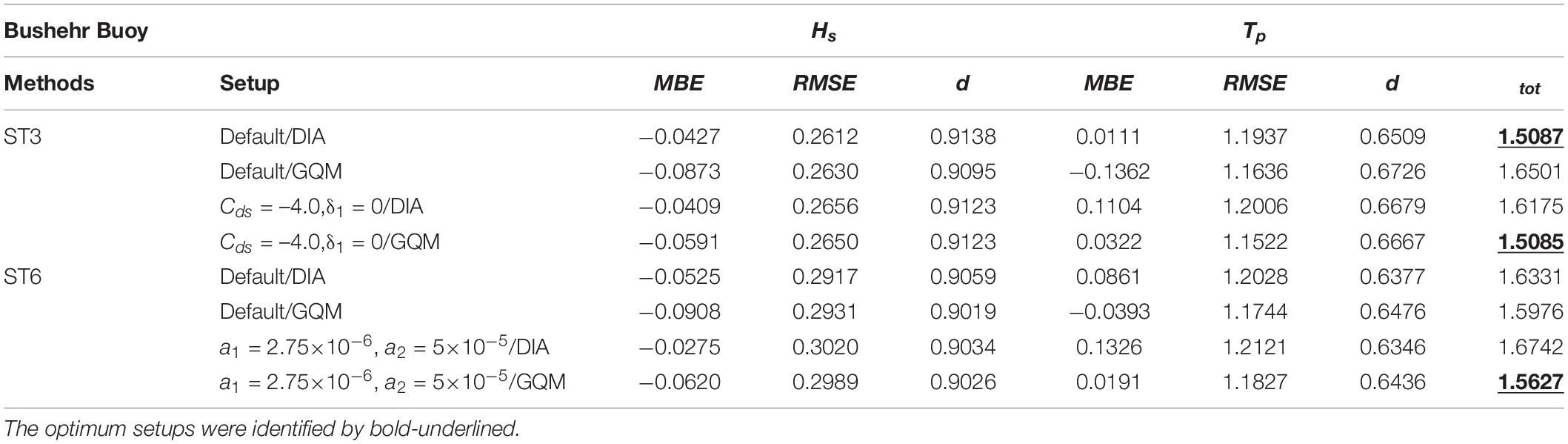
Table 3. The ST3 and ST6 packages using EXP4 wind data with two methods DIA and GQM for S_nl term were evaluated against buoy measured data at Bushehr.

Following results inferred from Table 3: (1) use of calibrated values for C_ds and δ₁ (C_ds = -4 and δ₁ = 0) with the GQM were resulted in _tot = 1.5085 which was identical to the employment of default values (C_ds = −4.5 and δ₁ = 0.5) and the DIA method (_tot = 1.5087). The value of δ₁ = 0 with the GQM was in agreement with the findings of Rogers et al. (2003). Default tuning values in S_ds term with the GQM and calibrated tuning values for S_ds term with the DIA method for S_nl term were the worst cases with highest _tot. (2) Similar to ST3, obtained tuning values (a₁ = 2.75×10⁻⁶, a₂ = 5×10⁻⁵) for ST6 when the GQM was considered for S_nl term were lower than default values (a₁ = 4.75×10⁻⁶, a₂ = 7×10⁻⁵). The GQM using calibrated values outperformed other setups according to _tot; the improvement was marginal compared to the DIA method with default values though.

The wave spectrum evolution simulated by ST3 and ST6 packages using the GQM and DIA methods were compared in Figure 12. Based on results presented in Table 3, default tuning values for white capping terms were applied in combination with the DIA, while calibrated values were considered when the GQM was employed. The highest energy density occurred during 16–17 March. The GQM method in the model has resulted in sharper peaks in the spectrum than the DIA method. As shown in several studies, the spectral peak was estimated smoother and lower than reality by the DIA (Gagnaire-Renou et al., 2010; Rogers and Van Vledder, 2013), and the GQM could improve this deficiency in the wave model.

FIGURE 12

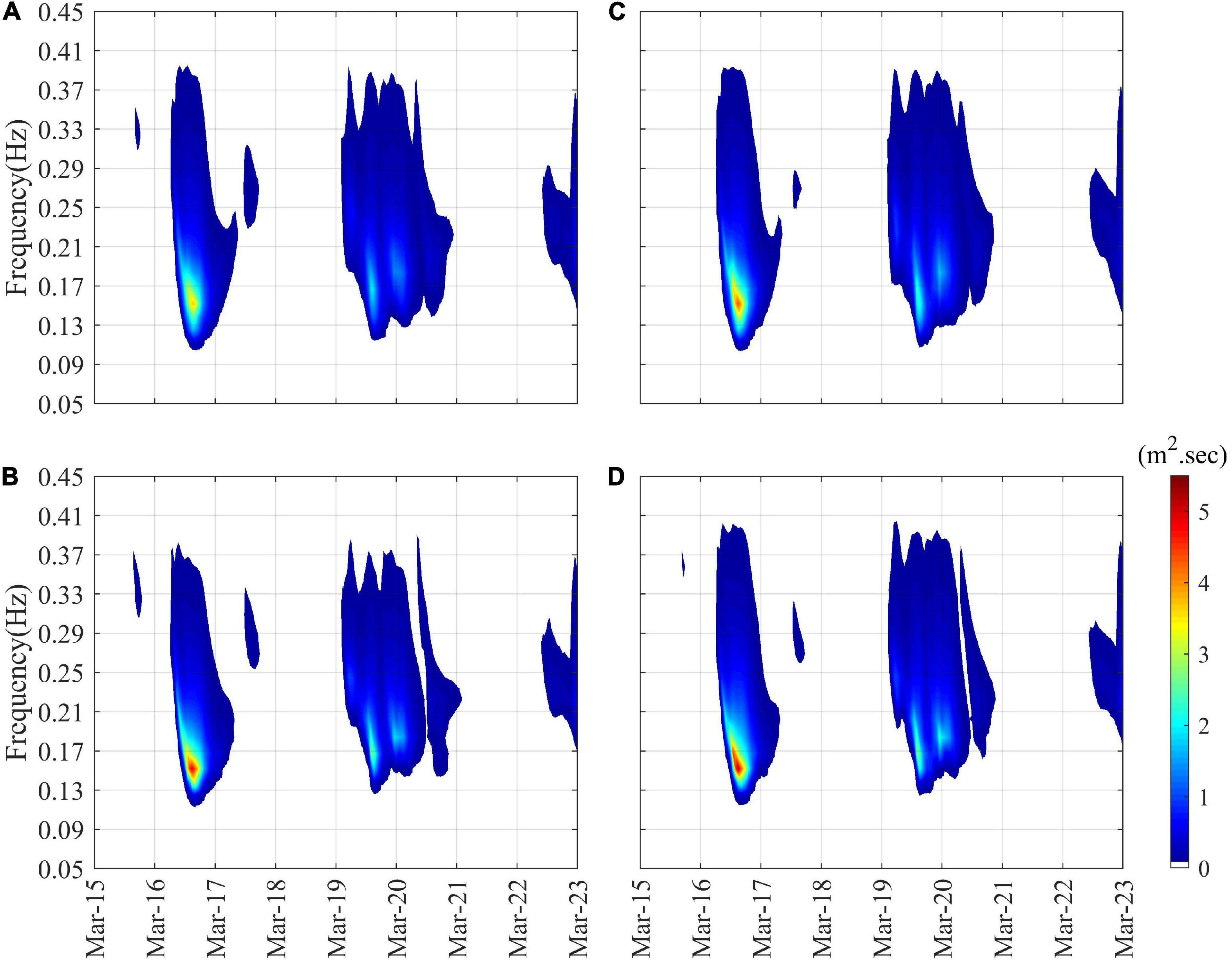
Figure 12. The wave spectrum evolution by ST3 (A,B) and ST6 (C,D). Snl was calculated with the DIA method in panels (A,C) and with the GQM method in panels (B,D).

The energy content close to the peak of the spectrum was also more intense for ST6 Than ST3. During the high energy event of 16–17 March, ST6 resulted in higher energy content, even in the high-frequency tail of the spectrum. It is following the results of Kalourazi et al. (2020) who compared different formulations during hurricane Ivan’s passage over the Gulf of Mexico. This pattern was also confirmed by ideal and field tests in previous studies (e.g., Zieger et al., 2015; van Vledder et al., 2016). Having more energetic predictions over the entire frequency band also occurred for other events during 19–20 March when ST6 with the GQM was used as compared with other combinations.

The main reason for deviation in the model performance by ST3 and ST6 packages could be explained by the contribution of S_in, S_ds, and S_nl terms to S_tot in Eq. (1). The spectrum evolution of S_tot (not shown here) indicates that the energy content is close to the peak of S_tot was higher for ST6 than for ST3. This explains the peak wave period overestimation by ST6. Also, when the GQM was used for S_nl instead of DIA, a concentrated positive lobe at slightly higher frequencies occurred. Furthermore, the negative lobe was less extended to higher frequencies for the GQM than for the DIA method. As a consequence, more energy is transferred to high frequencies when GQM was employed which alleviated the wave peak period overestimation.

Conclusion

Ensemble prediction is a practical approach to handle uncertainties in numerical model predictions. This is essential during complex meteorological conditions such as meteotsunamis due to the importance of small-scale atmospheric processes (Mourre et al., 2021). This study skill assessed the performance of the WRF physics ensemble of a high-resolution modeling system in retrieving atmospheric processes which led to recent meteotsunami in the Persian Gulf. Numerical experiments with initial and boundary conditions driven from the ECMWF IFS CY41r2 high-resolution operational analysis database were used to study the detailed representation of surface air pressure and wind speed during 15–23 March 2017 in the Persian Gulf. Six experiments were used with 2 microphysics (Thompson and WSM6), 3 cumulus physics schemes (New Tiedtke, Kain-Fritsch, and Grell–Devenyi), and 3 planetary boundary layer schemes (YSU, MYJ, and MYNN) along with Goddard and RRTM as short-wave and long-wave radiation schemes.

Using Mellor-Yamada-Nakanishi-Niino scheme for planetary boundary layer and surface layer, EXP3 and EXP4 parameterizations overestimated surface pressure at the ground level stations and underestimated the wind speed. However, for stations inside the water body, it results to lower surface pressure and relatively higher wind speed compared to other experiments. The results indicated that combining MYNN planetary boundary layer scheme and the Thompson microphysics scheme provided the most reliable results for pressure and wind speed predictions. Also, wind speed is estimated better for either the MYJ or MYNN boundary layer scheme than non-local YSU during the Persian Gulf meteotsunami event. It implied that the turbulent eddies during this time period were small over the Persian Gulf and localized in nature. In general, EXP4 parameterization (using MYNN scheme for planetary boundary layer and surface layer) had the best performance at stations over water and EXP2 parameterization (using MYJ scheme for planetary boundary layer and Eta similarity for surface layer) had the best performance at stations on land.

Additional numerical experiments were performed to evaluate the sensitivity of WRF simulations to the selection of microphysics and convective parameterization using heat and moisture content in the atmosphere and maximum radar reflectivity. The results showed that all simulations were successful in reproducing temperature and moisture content in the atmosphere, but they overestimated the moisture content in the upper troposphere. Also, simulations with WSM6 microphysics produced slightly stronger reflectivity, especially at the southern part of the domain. Radar data indicated that in that area, both WSM6 and Thompson microphysics provided excessive reflectivity.

Both ST3 and ST6 packages in the WWIII model were used with six WRF experiments and ERA5 wind data to reproduce H_s and T_p during 15–23 March 2017. Two sets of tuning parameters were used when ERA5 wind data were used: (1) default tuning values; (2) calibrated tuning values proposed by BSD2021. Buoy measurements at Bushehr were used for model assessments. A new error parameter was introduced to determine the most suitable wind data for the wave model during the dominance of meteotsunami in the Persian Gulf. The lowest error was obtained when wind data were produced by the EXP4 parameterization. The ERA5 data led to the severe underestimation of H_s and T_p in the model.

For the first time, the exact GQM was implemented in the WWIII model to compensate for the deficiencies of the DIA in deep water. The GQM could be faster than available exact solutions in the third-generation wave models. The preliminary calibration of tuning parameters for S_ds the term was performed when the GQM was applied for S_nl term in the wave model. It is inferable that slightly better performances of the model relative to the DIA method were achieved when lower tuning values were applied.

Conducting two-way coupling between atmosphere, ocean, and wave models using the new implemented S_nl term for reproducing meteotsunami forerunner longwave and its interaction with high-frequency wind waves would be the next step to better study this meteotsunami event.

Data Availability Statement

The data analyzed in this study is subject to the following licenses/restrictions: Part of data comes from Iran Meteorological Organization and the Port and Maritime Organization (PMO) of Iran; and any user should directly asked data from them. ERA5 data can be downloaded directly from their website. Requests to access these datasets should be directed to https://marinedata.pmo.ir/; https://cds.climate.copernicus.eu/cdsapp#!/search?type=dataset.

Author Contributions

MR and SS contributed to conception and design of the study. MR performed WRF and COAWST simulations while MB performed wave modeling. MR and MB provided the first draft of the manuscript and it was finalized by SS. All authors contributed to manuscript revision, read, and approved the submitted version.

Conflict of Interest

The authors declare that the research was conducted in the absence of any commercial or financial relationships that could be construed as a potential conflict of interest.

Publisher’s Note

All claims expressed in this article are solely those of the authors and do not necessarily represent those of their affiliated organizations, or those of the publisher, the editors and the reviewers. Any product that may be evaluated in this article, or claim that may be made by its manufacturer, is not guaranteed or endorsed by the publisher.

Acknowledgments

We thank the Iran Meteorological Organization for providing synoptic data. The wave buoys data were provided by the Port and Maritime Organization (PMO) of Iran, respectively. ERA5 reanalysis data were downloaded from the ECMWF dataset. We should appreciate Eftekhari who revisited the manuscript from the point of view of the English proficiencies.

Footnotes

1. ^ http://www.pmo.ir/en/home
2. ^ http://weather.uwyo.edu
3. ^ http://www.ecmwf.int/en/forecasts/datasets/reanalysis-datasets/era5
4. ^ https://github.com/wrf-model/WRF
5. ^ http://rda.ucar.edu/datasets/ds113.1
6. ^ https://github.com/wrf-model/WPS/releases

References

Akbari, P., Sadrinasab, M., Chegini, V., and Siadatmousavi, M. (2016). Tidal constituents in the Persian Gulf, Gulf of Oman and Arabian Sea: a numerical study. Indian J. Geo Mar. Sci. 45, 1010–1016.

Google Scholar

Al-Hajri, K. R. (1990). The Circulation of the Arabian (Persian) Gulf: a Model Study of its Dynamics. Washington, DC: The Catholic University of America.

Google Scholar

Ambraseys, N. N. (2008). “Descriptive catalogues of historical earthquakes in the Eastern Mediterranean and the Middle East; revisited,” in Historical Seismology, eds J. Frechet and M. Meghraoui (Berlin: Springer).

Google Scholar

Athar, H., and Ammar, K. (2016). Seasonal characteristics of the large-scale moisture flux transport over the Arabian Peninsula. Theor. Appl. Climatol. 124, 565–578. doi: 10.1007/s00704-015-1437-7

CrossRef Full Text | Google Scholar

Athukorala, R., Thol, T., Neluwala, P., Petri, M., Sengxeu, S., Lattada, L., et al. (2021). Evaluating the performance of a WRF physics ensemble in simulating rainfall over Lao PDR during wet and dry seasons. Adv. Meteorol. 2021:6630302. doi: 10.1155/2021/6630302

CrossRef Full Text | Google Scholar

Belušić, D., Grisogono, B., and Klaić, Z. B. (2007). Atmospheric origin of the devastating coupled air-sea event in the east Adriatic. J. Geophys. Res. Atmospheres 112:14. doi: 10.1029/2006JD008204

CrossRef Full Text | Google Scholar

Benoit, M. (2005). “Evaluation of methods to compute the non-linear quadruplet interactions for deep-water wave spectra,” in Proceedings 5th International Symposiumon Ocean Wave Measurement and Analysis (Israel: WAVES), 3–7.

Google Scholar

Benoit, M. (2007). “Implementation and Test of Improved Methods for Evaluation of Nonlinear Quadruplet Interactions in a Third Generation Wave Model,” in Coastal Engineering 2006, ed. J. M. Smith, Vol. 5. Singapore: World Scientific, 526–538. doi: 10.1142/9789812709554_0046

CrossRef Full Text | Google Scholar

Beyramzadeh, M., Siadatmousavi, S. M., and Derkani, M. H. (2021). Calibration and skill assessment of two input and dissipation parameterizations in WAVEWATCH-III model forced with ERA5 winds with application to Persian Gulf and Gulf of Oman. Ocean Eng. 219:108445. doi: 10.1016/j.oceaneng.2020.108445

CrossRef Full Text | Google Scholar

Borge, R., Alexandrov, V., Del Vas, J. J., Lumbreras, J., and Rodríguez, E. (2008). A comprehensive sensitivity analysis of the WRF model for air quality applications over the Iberian Peninsula. Atmos. Environ. 42, 8560–8574. doi: 10.1016/j.atmosenv.2008.08.032

CrossRef Full Text | Google Scholar

Cavaleri, L., and Bertotti, L. (2003). The characteristics of wind and wave fields modelled with different resolutions. Quart. J. R. Meteorol. Soc. 129, 1647–1662. doi: 10.1256/qj.01.68

CrossRef Full Text | Google Scholar

Cavaleri, L., and Bertotti, L. (2006). The improvement of modelled wind and wave fields with increasing resolution. Ocean Eng. 33, 553–565. doi: 10.1016/j.oceaneng.2005.07.004

CrossRef Full Text | Google Scholar

Chou, M.-D., and Suarez, M. J. (1994). An Efficient Thermal Infrared Radiation Parameterization for Use in General Circulation Models, NASA Tech. Memo. 104606. Linthicum Heights, MD: NASA Center for Aerospace Information, 85.

Google Scholar

Christakos, K., Björkqvist, J.-V., Tuomi, L., Furevik, B. R., and Breivik, Ø (2020). Modelling wave growth in narrow fetch geometries: the white-capping and wind input formulations. Ocean Model. 157:101730. doi: 10.1016/j.ocemod.2020.101730

CrossRef Full Text | Google Scholar

Denamiel, C., Šepić, J., Ivanković, D., and Vilibić, I. (2019). The Adriatic Sea and Coast modelling suite: evaluation of the meteotsunami forecast component. Ocean Model. 135, 71–93. doi: 10.1016/j.ocemod.2019.02.003

CrossRef Full Text | Google Scholar

Donelan, M. A., Babanin, A. V., Young, I. R., and Banner, M. L. (2006). Wave-follower field measurements of the wind-input spectral function. Part II: parameterization of the wind input. J. Phys. Oceanogr. 36, 1672–1689. doi: 10.1175/JPO2933.1

CrossRef Full Text | Google Scholar

El-Sabh, M., and Murty, T. (1989). Storm surges in the Arabian Gulf. Nat. Hazards 1, 371–385. doi: 10.1007/BF00134834

CrossRef Full Text | Google Scholar

Gagnaire-Renou, E., Benoit, M., and Forget, P. (2009). “Modeling waves in fetch-limited and slanting fetch conditions using a quasi-exact method for nonlinear four-wave interactions,” in Coastal Engineering 2008, Vol. 5, ed. J. M. Smith (Singapore: World Scientific), 496–508. doi: 10.1142/9789814277426_0042

CrossRef Full Text | Google Scholar

Gagnaire-Renou, E., Benoit, M., and Forget, P. (2010). Ocean wave spectrum properties as derived from quasi-exact computations of nonlinear wave-wave interactions. J. Geophys. Res. Oceans 115. doi: 10.1029/2009JC005665

CrossRef Full Text | Google Scholar

Grell, G. A., and Dévényi, D. (2002). A generalized approach to parameterizing convection combining ensemble and data assimilation techniques. Geophys. Res. Lett. 29. 38-31–38-34. doi: 10.1029/2002GL015311

CrossRef Full Text | Google Scholar

WAVEWATCH III Development Group WW3DG (2016). User Manual and System Documentation of Wavewatch III version 5.16. Technical Note 329. Washington, DC: NOAA

Google Scholar

Hasselmann, S., Hasselmann, K., Allender, J., and Barnett, T. (1985). Computations and parameterizations of the nonlinear energy transfer in a gravity-wave specturm. Part II: parameterizations of the nonlinear energy transfer for application in wave models. J. Phys. Oceanogr. 15, 1378–1391. doi: 10.1175/1520-0485(1985)015<1378:CAPOTN>2.0.CO;2

CrossRef Full Text | Google Scholar

Heidarzadeh, M., Pirooz, M. D., Zaker, N. H., Yalciner, A. C., Mokhtari, M., and Esmaeily, A. (2008). Historical tsunami in the Makran Subduction Zone off the southern coasts of Iran and Pakistan and results of numerical modeling. Ocean Eng. 35, 774–786. doi: 10.1016/j.oceaneng.2008.01.017

CrossRef Full Text | Google Scholar

Heidarzadeh, M., Šepić, J., Rabinovich, A., Allahyar, M., Soltanpour, A., and Tavakoli, F. (2020). Meteorological tsunami of 19 March 2017 in the Persian Gulf: observations and analyses. Pure Appl. Geophys. 177, 1231–1259. doi: 10.1007/s00024-019-02263-8

CrossRef Full Text | Google Scholar

Hong, S.-Y., and Lim, J.-O. J. (2006). The WRF single-moment 6-class microphysics scheme (WSM6). Asia Pac. J. Atmos. Sci. 42, 129–151.

Google Scholar

Hong, S.-Y., Noh, Y., and Dudhia, J. (2006). A new vertical diffusion package with an explicit treatment of entrainment processes. Mon. Weather Rev. 134, 2318–2341. doi: 10.1175/MWR3199.1

CrossRef Full Text | Google Scholar

Horvath, K., and Vilibić, I. (2014). “Atmospheric mesoscale conditions during the Boothbay meteotsunami: a numerical sensitivity study using a high-resolution mesoscale model,” in Meteorological Tsunamis: the US East Coast and Other Coastal Regions, eds I. Vilibic and S. Monserrat (Berlin: Springer), 55–74. doi: 10.1007/978-3-319-12712-5_4

CrossRef Full Text | Google Scholar

Horvath, K., Šepić, J., and Prtenjak, M. T. (2018). Atmospheric forcing conducive for the Adriatic 25 June 2014 meteotsunami event. Pure Appl. Geophys. 175, 3817–3837. doi: 10.1007/s00024-018-1902-1

CrossRef Full Text | Google Scholar

Janjić, Z. I. (1994). The step-mountain eta coordinate model: further developments of the convection, viscous sublayer, and turbulence closure schemes. Mon. Weather Rev. 122, 927–945. doi: 10.1175/1520-0493(1994)122<0927:TSMECM>2.0.CO;2

CrossRef Full Text | Google Scholar

Janssen, P. A. (1991). Quasi-linear theory of wind-wave generation applied to wave forecasting. J. Phys. Oceanogr. 21, 1631–1642. doi: 10.1175/1520-0485(1991)021<1631:QLTOWW>2.0.CO;2

CrossRef Full Text | Google Scholar

Jiménez, P. A., Dudhia, J., González-Rouco, J. F., Navarro, J., Montávez, J. P., and García-Bustamante, E. (2012). A revised scheme for the WRF surface layer formulation. Mon. Weather Rev. 140, 898–918. doi: 10.1175/MWR-D-11-00056.1

CrossRef Full Text | Google Scholar

Kain, J. S. (2004). The Kain–fritsch convective parameterization: an update. J. Appl. Meteorol. 43, 170–181. doi: 10.1175/1520-0450(2004)043<0170:TKCPAU>2.0.CO;2

CrossRef Full Text | Google Scholar

Kalourazi, M. Y., Siadatmousavi, S. M., Yeganeh-Bakhtiary, A., and Jose, F. (2020). WAVEWATCH-III source terms evaluation for optimizing hurricane wave modeling: a case study of Hurricane Ivan. Oceanologia 63, 194–213. doi: 10.1016/j.oceano.2020.12.001

CrossRef Full Text | Google Scholar

Kamranzad, B. (2018). Persian Gulf zone classification based on the wind and wave climate variability. Ocean Eng. 169, 604–635. doi: 10.1016/j.oceaneng.2018.09.020

CrossRef Full Text | Google Scholar

Kazeminezhad, M. H., Vilibić, I., Denamiel, C., Ghafarian, P., and Negah, S. (2021). Weather radar and ancillary observations of the convective system causing the northern Persian Gulf meteotsunami on 19 March 2017. Nat. Hazards 106, 1747–1769. doi: 10.1007/s11069-020-04208-0

CrossRef Full Text | Google Scholar

Komen, G., Cavaleri, L., Donelan, M., Hasselmann, K., Hasselmann, S., and Janssen, P. (1994). Dynamics and Modelling of Ocean Waves. Cambridge: Cambridge University Press. doi: 10.1017/CBO9780511628955

CrossRef Full Text | Google Scholar

Lavrenov, I. V. (2001). Effect of wind wave parameter fluctuation on the nonlinear spectrum evolution. J. Phys. Oceanogr. 31, 861–873. doi: 10.1175/1520-0485(2001)031<0861:EOWWPF>2.0.CO;2

CrossRef Full Text | Google Scholar

Liao, Y.-P., and Kaihatu, J. M. (2016). The effect of wind variability and domain size in the Persian Gulf on predicting nearshore wave energy near Doha. Qatar. Appl. Ocean Res. 55, 18–36. doi: 10.1016/j.apor.2015.11.012

CrossRef Full Text | Google Scholar

Lin, N., and Emanuel, K. (2016). Grey swan tropical cyclones. Nat. Clim. Change 6, 106–111. doi: 10.1038/nclimate2777

CrossRef Full Text | Google Scholar

Linares, Á, Wu, C. H., Bechle, A. J., Anderson, E. J., and Kristovich, D. A. R. (2019). Unexpected rip currents induced by a meteotsunami. Sci. Rep. 9. doi: 10.1038/s41598-019-38716-2

PubMed Abstract | CrossRef Full Text | Google Scholar

Liu, Q., Babanin, A., Fan, Y., Zieger, S., Guan, C., and Moon, I.-J. (2017). Numerical simulations of ocean surface waves under hurricane conditions: assessment of existing model performance. Ocean Model. 118, 73–93. doi: 10.1016/j.ocemod.2017.08.005

CrossRef Full Text | Google Scholar

Liu, Q., Rogers, W. E., Babanin, A. V., Young, I. R., Romero, L., Zieger, S., et al. (2019). Observation-based source terms in the third-generation wave model WAVEWATCH III: updates and verification. J. Phys. Oceanogr. 49, 489–517. doi: 10.1175/JPO-D-18-0137.1

CrossRef Full Text | Google Scholar

Mlawer, E. J., Taubman, S. J., Brown, P. D., Iacono, M. J., and Clough, S. A. (1997). Radiative transfer for inhomogeneous atmospheres: RRTM, a validated correlated-k model for the longwave. J. Geophys. Res. Atmos. 102, 16663–16682. doi: 10.1029/97JD00237

CrossRef Full Text | Google Scholar

Modarress, B., Ansari, A., and Thies, E. (2012). The effect of transnational threats on the security of Persian Gulf maritime petroleum transportation. J. Transportation Security 5, 169–186. doi: 10.1007/s12198-012-0090-y

CrossRef Full Text | Google Scholar

Monin, A. S., and Obukhov, A. M. (1954). Basic laws of turbulent mixing in the surface layer of the atmosphere. Contrib. Geophys. Inst. Acad. Sci. USSR 151:e187.

Google Scholar

Monserrat, S., Vilibić, I., and Rabinovich, A. B. (2006). Meteotsunamis: atmospherically induced destructive ocean waves in the tsunami frequency band. Nat. Hazards Earth Syst. Sci. 6, 1035–1051. doi: 10.5194/nhess-6-1035-2006

CrossRef Full Text | Google Scholar

Mourre, B., Santana, A., Buils, A., Gautreau, L., Lièer, M., Jansà, A., et al. (2021). On the potential of ensemble forecasting for the prediction of meteotsunamis in the Balearic Islands: sensitivity to atmospheric model parameterizations. Nat. Hazards 106, 1315–1336. doi: 10.1007/s11069-020-03908-x

CrossRef Full Text | Google Scholar

Nadim, F., Bagtzoglou, A. C., and Iranmahboob, J. (2008). Coastal management in the Persian Gulf region within the framework of the ROPME programme of action. Ocean Coast. Manag. 51, 556–565. doi: 10.1016/j.ocecoaman.2008.04.007

CrossRef Full Text | Google Scholar

Nakanishi, M., and Niino, H. (2006). An improved mellor–yamada level-3 model: its numerical stability and application to a regional prediction of advection fog. Boundary Layer Meteorol. 119, 397–407. doi: 10.1007/s10546-005-9030-8

CrossRef Full Text | Google Scholar

Nayak, S., Sandeepan, B., and Panchang, V. (2016). “Effect of high resolution winds on wind-wave simulations in Arabian Gulf,” in Qatar Foundation Annual Research Conference Proceedings Volume 2016 Issue 1, (Qatar: Hamad bin Khalifa University Press). doi: 10.5339/qfarc.2016.EEPP2869

CrossRef Full Text | Google Scholar

Niu, G.-Y., Yang, Z.-L., Mitchell, K. E., Chen, F., Ek, M. B., Barlage, M., et al. (2011). The community Noah land surface model with multiparameterization options (Noah-MP): 1. model description and evaluation with local-scale measurements. J. Geophys. Res. Atmos. 116:19. doi: 10.1029/2010JD015139

CrossRef Full Text | Google Scholar

Perrie, W., Toulany, B., Resio, D. T., Roland, A., and Auclair, J.-P. (2013). A two-scale approximation for wave–wave interactions in an operational wave model. Ocean Model. 70, 38–51. doi: 10.1016/j.ocemod.2013.06.008

CrossRef Full Text | Google Scholar

Rabinovich, A. B. (2020). Twenty-seven years of progress in the science of meteorological tsunamis following the 1992 Daytona Beach event. Pure Appl. Geophys. 177, 1193–1230. doi: 10.1007/s00024-019-02349-3

CrossRef Full Text | Google Scholar

Rabinovich, A. B., and Thomson, R. E. (2007). “The 26 December 2004 sumatra tsunami: analysis of tide gauge data from the world ocean Part 1. Indian Ocean and South Africa,” in Tsunami and its Hazards in the Indian and Pacific Oceans, eds K. Staake, E. A. Okal, and J. C. Borrero (Berlin: Springer), 261–308. doi: 10.1007/978-3-7643-8364-0_2

CrossRef Full Text | Google Scholar

Renault, L., Vizoso, G., Jansá, A., Wilkin, J., and Tintoré, J. (2011). Toward the predictability of meteotsunamis in the Balearic sea using regional nested atmosphere and ocean models. Geophys. Res. Lett. 38:7. doi: 10.1029/2011GL047361

CrossRef Full Text | Google Scholar

Resio, D. T., and Perrie, W. (2008). A two-scale approximation for efficient representation of nonlinear energy transfers in a wind wave spectrum. Part I: theoretical development. J. Phys. Oceanogr. 38, 2801–2816. doi: 10.1175/2008JPO3713.1

CrossRef Full Text | Google Scholar

Reynolds, R. M. (1993). Physical oceanography of the Gulf, Strait of Hormuz, and the Gulf of oman—results from the Mt Mitchell expedition. Mar. Pollut. Bull. 27, 35–59. doi: 10.1016/0025-326X(93)90007-7

CrossRef Full Text | Google Scholar

Rogers, W. E., and Van Vledder, G. P. (2013). Frequency width in predictions of windsea spectra and the role of the nonlinear solver. Ocean Model. 70, 52–61. doi: 10.1016/j.ocemod.2012.11.010

CrossRef Full Text | Google Scholar

Rogers, W. E., Babanin, A. V., and Wang, D. W. (2012). Observation-consistent input and whitecapping dissipation in a model for wind-generated surface waves: description and simple calculations. J. Atmos. Oceanic Technol. 29, 1329–1346. doi: 10.1175/JTECH-D-11-00092.1

CrossRef Full Text | Google Scholar

Rogers, W. E., Hwang, P. A., and Wang, D. W. (2003). Investigation of wave growth and decay in the SWAN model: three regional-scale applications. J. Phys. Oceanogr. 33, 366–389. doi: 10.1175/1520-0485(2003)033<0366:IOWGAD>2.0.CO;2

CrossRef Full Text | Google Scholar

Salaree, A., Mansouri, R., and Okal, E. A. (2018). The intriguing tsunami of 19 March 2017 at Bandar Dayyer, Iran: field survey and simulations. Nat. Hazards 90, 1277–1307. doi: 10.1007/s11069-017-3119-5

CrossRef Full Text | Google Scholar

Šepić, J., and Rabinovich, A. B. (2014). “Meteotsunami in the Great Lakes and on the Atlantic coast of the United States generated by the “derecho” of June 29–30, 2012,” in Meteorological Tsunamis: the US East Coast and Other Coastal Regions, eds I. Vilibic, S. Monserrat, and A. B. Rabinovich (Berlin: Springer), 75–107. doi: 10.1007/978-3-319-12712-5_5

CrossRef Full Text | Google Scholar

Šepić, J., Vilibić, I., and Belušić, D. (2009). Source of the 2007 Ist meteotsunami (Adriatic Sea). J. Geophys. Res. Oceans 114:14. doi: 10.1029/2008JC005092

CrossRef Full Text | Google Scholar

Šepić, J., Vilibić, I., Rabinovich, A. B., and Monserrat, S. (2015). Widespread tsunami-like waves of 23-27 June in the Mediterranean and Black Seas generated by high-altitude atmospheric forcing. Sci. Rep. 5:11682. doi: 10.1038/srep11682

PubMed Abstract | CrossRef Full Text | Google Scholar

Shi, L., Olabarrieta, M., Nolan, D. S., and Warner, J. C. (2020). Tropical cyclone rainbands can trigger meteotsunamis. Nat. Commun. 11:678. doi: 10.1038/s41467-020-14423-9

PubMed Abstract | CrossRef Full Text | Google Scholar

Shi, L., Olabarrieta, M., Valle-Levinson, A., and Warner, J. C. (2019). Relevance of wind stress and wave-dependent ocean surface roughness on the generation of winter meteotsunamis in the Northern Gulf of Mexico. Ocean Model. 140:101408. doi: 10.1016/j.ocemod.2019.101408

CrossRef Full Text | Google Scholar

Siadatmousavi, S. M., Jose, F., and Stone, G. (2012). On the importance of high frequency tail in third generation wave models. Coast. Eng. 60, 248–260. doi: 10.1016/j.coastaleng.2011.10.007

CrossRef Full Text | Google Scholar

Skamarock, C., Klemp, B., Dudhia, J., Gill, O., Liu, Z., Berner, J., et al. (2019). A Description of the Advanced Research WRF Model Version 4.

Google Scholar

Taylor, K. E. (2001). Summarizing multiple aspects of model performance in a single diagram. J. Geophys. Res. Atmos. 106, 7183–7192. doi: 10.1029/2000JD900719

CrossRef Full Text | Google Scholar

Thompson, G., Field, P. R., Rasmussen, R. M., and Hall, W. D. (2008). Explicit forecasts of winter precipitation using an improved bulk microphysics scheme. Part II: implementation of a new snow parameterization. Mon. Weather Rev. 136, 5095–5115. doi: 10.1175/2008MWR2387.1

CrossRef Full Text | Google Scholar

Thoppil, P. G., and Hogan, P. J. (2010). Persian Gulf response to a wintertime shamal wind event. Deep Sea Res. Part I Oceanogr. Res. Papers 57, 946–955. doi: 10.1016/j.dsr.2010.03.002

CrossRef Full Text | Google Scholar

van Vledder, G. P., Hulst, S. T. C., and McConochie, J. D. (2016). Source term balance in a severe storm in the Southern North Sea. Ocean Dyn. 66, 1681–1697. doi: 10.1007/s10236-016-0998-z

CrossRef Full Text | Google Scholar

Vilibić, I., Monserrat, S., Rabinovich, A., and Mihanović, H. (2008). Numerical Modelling of the Destructive Meteotsunami of 15 June, 2006 on the Coast of the Balearic Islands. Pure Appl. Geophys. 165, 2169–2195. doi: 10.1007/s00024-008-0426-5

CrossRef Full Text | Google Scholar

Vilibić, I., Šepić, J., Rabinovich, A. B., and Monserrat, S. (2016). Modern approaches in Meteotsunami research and early warning. Front. Mar. Sci. 3:57. doi: 10.3389/fmars.2016.00057

CrossRef Full Text | Google Scholar

Williams, D. A. (2020). Meteotsunami Generation, Amplification and Occurrence in North-West Europe. England: The University of Liverpool.

Google Scholar

Willmott, C. J. (1982). Some comments on the evaluation of model performance. Bull. Am. Meteorol. Soc. 63, 1309–1313. doi: 10.1175/1520-0477(1982)063<1309:SCOTEO>2.0.CO;2

CrossRef Full Text | Google Scholar

Zhang, C., and Wang, Y. (2017). Projected future changes of tropical cyclone activity over the Western North and South Pacific in a 20-km-mesh regional climate model. J. Clim. 30, 5923–5941. doi: 10.1175/JCLI-D-16-0597.1

CrossRef Full Text | Google Scholar

Zieger, S., Babanin, A. V., Rogers, W. E., and Young, I. R. (2015). Observation-based source terms in the third-generation wave model WAVEWATCH. Ocean Model. 96, 2–25. doi: 10.1016/j.ocemod.2015.07.014

CrossRef Full Text | Google Scholar