Uncertainties Associated With Simulating Regional Sea Surface Height and Tides: A Case Study of the East China Seas

Jiang, Long; Lu, Xinyu; Xu, Wenlong; Yao, Peng; Cheng, Xuhua

doi:10.3389/fmars.2022.827547

ORIGINAL RESEARCH article

Front. Mar. Sci., 02 March 2022

Sec. Coastal Ocean Processes

Volume 9 - 2022 | https://doi.org/10.3389/fmars.2022.827547

Uncertainties Associated With Simulating Regional Sea Surface Height and Tides: A Case Study of the East China Seas

$\r\nLong Jiang,,*$ Long Jiang^1,2,3*

Xinyu Lu²

Wenlong Xu²

Peng Yao^4* $Xuhua Cheng,\r\n$ Xuhua Cheng^1,2

¹Key Laboratory of Marine Hazards Forecasting, Ministry of Natural Resources, Hohai University, Nanjing, China
²College of Oceanography, Hohai University, Nanjing, China
³Key Laboratory of Ministry of Education for Coastal Disaster and Protection, Hohai University, Nanjing, China
⁴College of Harbor, Coastal and Offshore Engineering, Hohai University, Nanjing, China

Modeling sea surface height (SSH) and tides is important but challenging in shelf seas. The Eastern China Seas (ECSs) is such a shelf sea with large inter-model deviations in prior studies. In order to assess and compare the possible uncertainty sources, numerical scenarios of varying the open boundary forcing, bottom roughness length scale, atmospheric forcing, grid resolution, and regional bathymetry were conducted in a hydrodynamic model of the ECSs. Results indicate that bathymetry data and open boundary forcing with inadequate accuracy generate uncertainties in SSH and tides locally and throughout the basin. An increase in bottom roughness enhances tidal dissipation and shifts amphidromes to the left relative to the incoming Kelvin waves, causing SSH variations in the ECSs. Refining the model resolution from 4 to 2 km mainly affects nearshore SSH and tides due to minor changes in depicted coastlines. Using different reanalysis meteorological data appears more important on the episodic than annual scale. It is highlighted that some uncertainty sources have opposing effects on SSH or tides and counteract their individual biases, making it difficult to achieve a realistic simulation. For example, increasing bottom roughness can not only compensate effects of overestimated tidal amplitude at open boundaries, but also balance out the overestimated M2 phase along the West Coast of Korea in a coarser-resolution model. Based on findings in this study, suggestions are provided for further reducing uncertainties in SSH and tide modeling in the ECSs and other shelf seas.

Introduction

Accurate simulation of tides and sea surface height (SSH) in regional seas is crucial to operational ocean forecasting systems benefiting maritime voyage, marine engineering, shoreline protection, and coastal recreational and economical activities (Zijl et al., 2013). In addition to forecasting models, simulating SSH is fundamental in any hydrodynamic models to correctly resolving the barotropic pressure gradient, current velocity, and heat/salt transport (Sannino et al., 2004). Therefore, achieving a high model skill in SSH is a fundamental step in calibration and validation of a hydrodynamic model (Xia et al., 2006; Ge et al., 2013).

Variations of the real-time SSH are associated with tides, wind surges, river runoff, baroclinic processes, eddies, ocean circulation, climate change, and non-linear interactions of these processes, etc. (Cheng et al., 2013, 2017; Müller et al., 2014). In coastal and shelf seas, tides and wind forcing usually dominate the changes in SSH (Teague et al., 1998; Wang et al., 2009; Zijl et al., 2013). While the SSH prediction in global models becomes increasingly accurate due to the extensive assimilation of satellite altimetry data and advancement in dynamical modeling (Hart-Davis et al., 2021; Lyard et al., 2021), the shelf and coastal regions are always associated with large deviations in SSH and tides (Stammer et al., 2014).

For local interest, regional SSH and tide simulations are usually forced with the aforementioned global models as open boundaries and facilitated with finer model resolution and locally tuned model parameters (Aldridge and Davies, 1993; Lee et al., 2002; Zu et al., 2008; Thiébot et al., 2020a). Data assimilation and improved hydrodynamic model settings are primary solutions to reduce the local SSH uncertainties (Blain, 1997; Greenberg et al., 2007; Liu and Gan, 2016; Feng et al., 2019). Factors including the spatial resolution (Falcão et al., 2013), bathymetry (Quaresma and Pichon, 2013), open boundary forcing (Carter and Merrifield, 2007), bottom friction coefficients (Lee and Jung, 1999), and atmospheric forcing (Santoro et al., 2013) are potential sources of SSH and tide uncertainties in hydrodynamic models. Data assimilation cannot eliminate uncertainties from all sources (Lyard et al., 2006; Stammer et al., 2014). The relative importance of these factors seems to vary in different systems and models (Abdennadher and Boukthir, 2006; Yao et al., 2012; Lee et al., 2013). In order to achieve high model skills in SSH and tide simulations and to provide reference for subsequent data assimilation (e.g., the selection and priority of parameters for optimization), a comprehensive assessment of these uncertainty sources is highly essential but relatively limited in prior studies. Many studies focus on only a couple of them (e.g., Lardner et al., 1993; Shulman et al., 1998; Lu and Zhang, 2006; Nguyen and Lee, 2020).

In this study, we present a non-assimilative barotropic hydrodynamic model for SSH and tide simulation in the East China Seas (ECSs), a region with substantial inter-model deviations compared to other shelf seas (Stammer et al., 2014; Su et al., 2015). By comparing the modeled results to tide gauge data, influences of the open boundary forcing, bottom roughness length scale, atmospheric forcing, model resolution, and regional bathymetry on SSH and tide simulations were examined in order to discern the most important/sensitive sources of uncertainties. This study aims to provide suggestions for improving the SSH and tide modeling skills in the ECSs as well as reference for other shelf and coastal regions.

Study Area

The ECSs, consisting of the Bohai, Yellow, and East China Seas, are semi-enclosed marginal seas surrounded by China, North and South Korea, and Japan (Figure 1). This region is connected to the South China Sea through the Taiwan Strait, adjacent to the Pacific Ocean and Sea of Japan to its southeast and east, respectively (Figure 1). Most of the ECSs are continental shelf seas with decreasing water depth northwestwards and an average depth of ∼218 m.

FIGURE 1

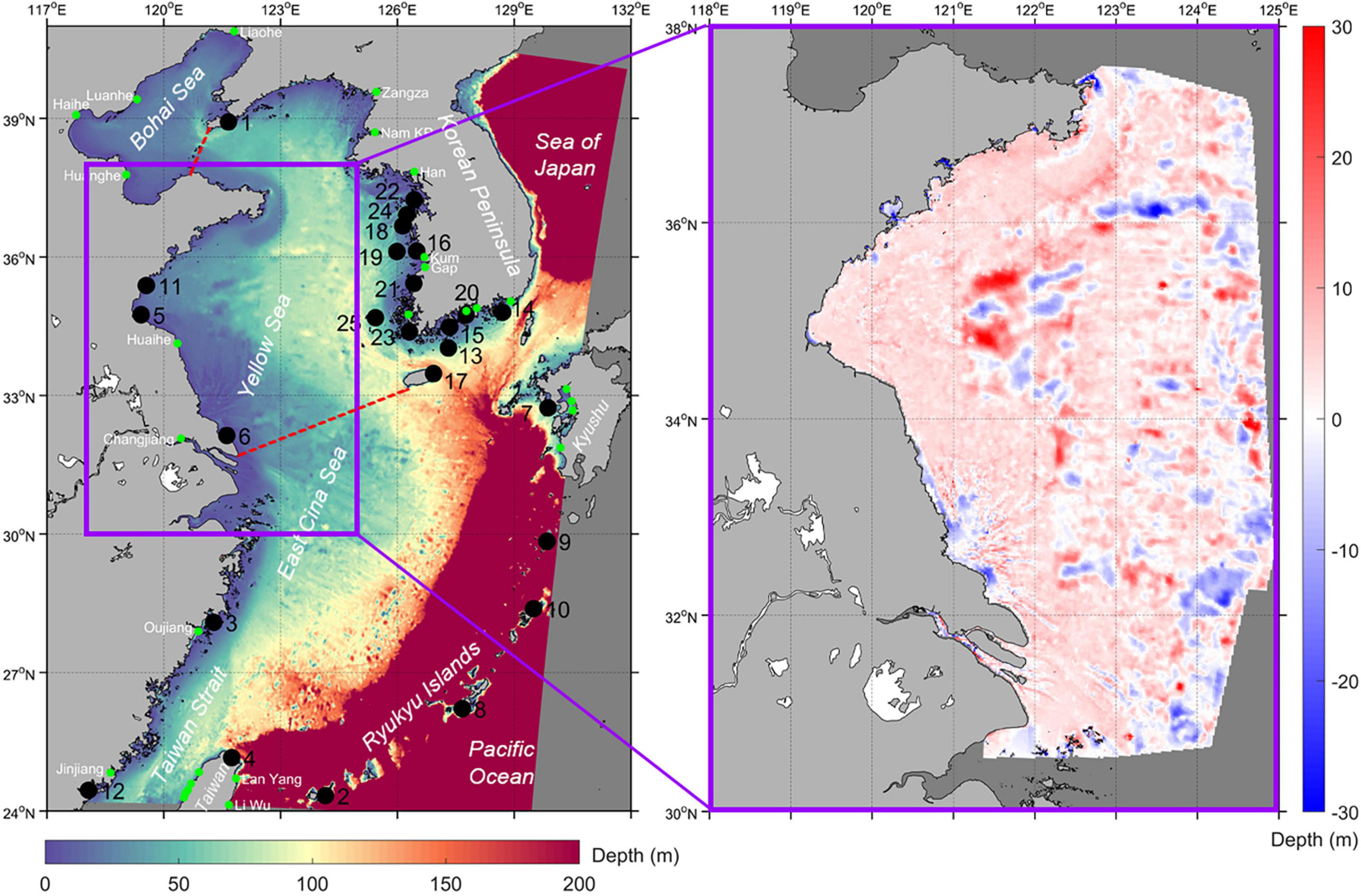
Figure 1. The study area with locations of tide gauges (black dots). The Bohai, Yellow, and East China Seas are separated with the red dashed lines. The river boundaries in the model are marked with the green dots. Rivers on the East Coast of Taiwan from north to south are Tou Chien, Hou Lung, Ta An, Ta Chia, and Tan Shui, respectively. Rivers on the South Coast of the Korean Peninsula from west to east are Yeong San, Somjin, Nam KR, and Nagdong, respectively. Rivers on the Kyushu Island from north to south are Chikugo, Kikuchi, Midori, and Kawabe, respectively. The right panel is a zoom-in view of the difference between the refined and GEBCO_2019 (shown on the left panel) bathymetry in the southwestern Yellow Sea. See names of the numbered tide gauges in section “Comparison of the Modeled and Observational Sea Surface Heights.”

The ECSs is one of the marginal seas with strongest tidal dissipation, accounting for 5–10% of the global total (Munk and Wunsch, 1998; Matsumoto et al., 2000; Yao et al., 2012). Tides exert a large influence on the SSH projection in the ECSs (Nguyen and Lee, 2020). Tidal waves dominated by semidiurnal components from the Pacific propagate into the ECSs through the Ryukyu Islands, the island chain between Taiwan and Kyushu (Figure 1), and are amplified and dissipated in the shallow coastal regions (Fang, 1979). Four principal tidal constituents are M2, S2, K1, and O1 with descending amplitude, respectively (Fang et al., 2004). Several amphidromic systems are generated due to the reflection of Kelvin waves in the semi-enclosed ECSs (An, 1977; Yanagi and Inoue, 1994; Bao et al., 2001). The largest tidal range mainly appears along the West Coast of the Korean Peninsula (Guo and Yanagi, 1998; Fang et al., 2004).

Winds dominate the detided variation in SSH in the ECSs (Teague et al., 1998). Controlled by the Eastern Asian monsoon, stronger (7.5–8.3 m/s on average) northwesterlies to northerlies prevail in winter and weaker (4.5–7.0 m/s on average) southwesterlies to southeasterlies in summer in this region (Hwang et al., 1999), with large interannual variability (Zhu et al., 2005). Typhoons that usually occur from July to October complicate the SSH variations. For example, the Super Typhoon Lekima in 2019 interacted with the astronomical tide and gave rise to an up-to-3-m storm surge in shallow waters (Wu et al., 2021).

Materials and Methods

Model Description

SSH in the ECSs was simulated with the open-source General Estuarine Transport Model (GETM)¹ that has been widely applied in coastal and shelf seas (van der Molen et al., 2016; Jiang et al., 2019; Chrysagi et al., 2021). GETM solves the finite-difference approximation of Reynolds-averaged Navier-Stokes equations with the hydrostatic assumption and turbulence closure model GOTM (General Ocean Turbulence Model). GETM includes a thin-layer scheme accurately simulating flooding and drying of tidal flats (Duran-Matute et al., 2014), which is important in the Bohai and Yellow Seas. We will focus on GETM settings related to the SSH simulation in this study and refer to its user manual on its website for further GETM descriptions.

Our model setup covers the ECSs and part of the adjacent Sea of Japan and Pacific Ocean (Figure 1) on a 2 km × 2 km Cartesian grid. In contrast to the spherical grid, in which the grid cell of certain longitude in the north is smaller than in the south, the Cartesian grid was applied to guarantee that the coastline and nearshore bathymetry all over the domain have the same spatial resolution. The UTM (Universal Transverse Mercator) coordinates were converted from longitude/latitude referring to the World Geodetic System 1984 (WGS84). The bathymetry data were interpolated from the General Bathymetric Chart of the Oceans, release 2019 (GEBCO_2019), accessible at https://www.gebco.net. GETM was run on a two-dimensional barotropic mode because of negligible impacts of baroclinic processes on SSH variations reported previously in this region (Guo and Yanagi, 1998; Yao et al., 2012; Feng et al., 2019). River discharge obtained from the Global River Discharge online dataset² was imposed on the river boundaries (Figure 1). SSH and barotropic currents were acquired from the FES2014 (Finite Element Solution 2014) global ocean tide atlas (Lyard et al., 2021) and imposed on the GETM Flather-type open boundaries (Figure 1). The 1/16° FES2014 assimilates SSH data of tidal gauges and satellite altimetry and includes 34 tidal components.³ Based on our prior test, the depth-average residual currents at the open boundary have a minimal effect on the tide and SSH in the domain and are omitted in all model runs. GETM calculates the non-uniform depth-related quadratic drag coefficient C_d based on the input of the bottom roughness length scale z₀ (Equation 1; Blumberg and Mellor, 1987).

C_{d} = \frac{κ^{2}}{\ln^{2} (\frac{z}{z_{0}})}, (1)

In Equation 1, κ is the von Kármán constant (approximately 0.41) and z is the water depth. For lack of spatial bottom boundary layer data (discussed in section “Recommendations for Future Endeavors”), we set a constant bottom roughness length scale (z₀ = 0.05 mm) according to the range of prior studies (e.g., Feng et al., 2019). The hourly ERA5 (ECMWF Reanalysis v5) meteorological data including air pressure and wind forcing were obtained from the European Centre for Medium-Range Weather Forecasts (ECMWF)⁴ and imposed on the model.

Model Scenarios

Five sets of model scenarios were conducted to assess influences of the open boundary forcing, bottom roughness length scale, atmospheric forcing, model resolution, and regional bathymetry on SSH and tide simulations (Table 1). In the Scenarios Obd1 and Obd2 (Table 1), open boundary forcing was extracted from two alternative global tide models: the TPXO9.v2 version of the OSU Tidal Prediction Software (OTPS, Egbert and Erofeeva, 2002)⁵ and the regional tide solution NAO99Jb version 2004.10.25 by the National Astronomical Observatory of Japan (Matsumoto et al., 2001),⁶ respectively. OTPS produces a state-of-the-art global tide atlas with a local resolution of 1/30°, 15 tidal constituents, altimetry and tide gauge data assimilated, and has improved its tide prediction skills over the past decades (Stammer et al., 2014; Lyard et al., 2021). Nested with a global tide model NAO99b solving 16 tidal constituents, NAO99Jb is a regional application of the Northwest Pacific with a resolution of 1/12°, which, assimilating SSH of the Topex/Poseidon altimetry and 219 coastal tidal gauges, shows relatively high accuracy in representing semidiurnal tides in the ECSs (Matsumoto et al., 2001; Feng et al., 2019; Nguyen and Lee, 2020).

TABLE 1

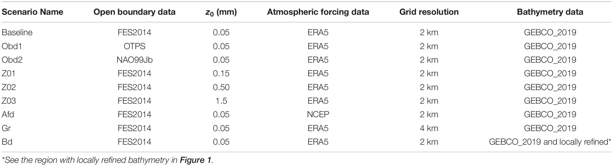
Table 1. Model scenarios in this study.

The roughness length z₀ was varied in the literature range 0.05–1.5 mm (Mofjeld, 1988; Lu and Zhang, 2006; Feng et al., 2019; Thiébot et al., 2020b) in Scenarios Baseline, Z1, Z2, and Z3 (Table 1). As calculated from Equation 1, the drag coefficient C_d in these scenarios increases with z₀ and decreases with water depth (Figure 2).

FIGURE 2

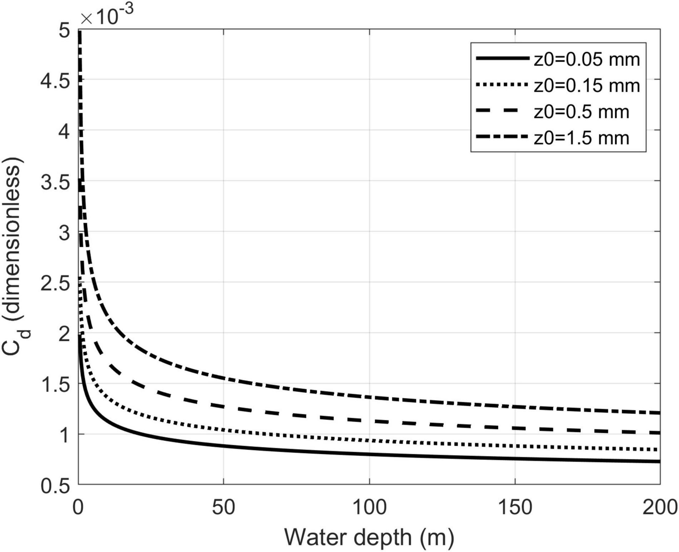
Figure 2. Relationship between bottom roughness C_d and bottom roughness length scale z₀ in seawater up to 200 m deep.

To compare with the ERA5 atmospheric forcing, we applied another set of meteorological input extracted from the Climate Forecast System v2 reanalysis data⁷ by NCEP (the National Centers for Environmental Prediction). The spatial resolution of the ERA5 and NCEP atmospheric data is 0.25° and 0.5°, respectively.

The model was also run on a 4 × 4 km grid with other settings identical to the baseline scenario (Scenario Gr in Table 1) in order to examine how the grid resolution may affect the SSH simulation.

Despite a high spatial resolution (15 arc-second), the GEBCO_2019 bathymetry is not always accurate in coastal waters. To differentiate from the baseline scenario, we applied bathymetry data that are locally measured as well as digitalized from the official marine charts published by the Maritime Safety Administration of China (Yao, 2016) to the Scenario Bd (Table 1). The locally refined bathymetry, despite not covering the entire model domain (Figure 1), can provide insight into influences of bathymetry on SSH and tide predictions.

Comparison of the Modeled and Observational Sea Surface Heights

To evaluate the SSH uncertainties in the aforementioned scenarios, model results were compared with SSH measured at the Chinese, Korean, and Japanese tide gauges (Figure 1). The hourly SSH at the Chinese (data range: 1985–1990 except for Keelung, 2013–2019) and Japanese (data range: 2013–2019) tide gauges were obtained from the University of Hawaii Sea Level Center database (UHSLC).⁸ The Korean tide gauges (data range: 2013–2019) were downloaded from Korea Hydrographic and Oceanographic Agency.⁹ To accommodate with the observational SSH, the model was run for the years 1985–1990 and 2013–2019.

Data gaps lasting days or months are common in the observational SSH time series. For each tide gauge, we selected 1-year data with the fewest data gaps for comparison against the model simulation: (1) Dalian, 1988; (2) Ishigaki, 1986; (3) Kanmen, 1988; (4) Keelung, 1987; (5) Lianyungang, 1986; (6) Lusi, 1985; (7) Nagasaki, 1987; (8) Naha, 1989; (9) Nakano Shima, 1985; (10) Naze, 1986; (11) Shijiusuo, 1988; (12) Xiamen, 1985; (13) Geomundo, 2013; (14) Geoje, 2014; (15) Goheung, 2014; (16) Seocheonmaryang, 2019; (17) Seongsanpo, 2015; (18) Anheung, 2015; (19) Eocheongdo, 2014; (20) Yeosu, 2013; (21) Yeonggwang, 2019; (22) Yeongheungdo, 2015; (23) Jindo, 2015; (24) Taean, 2015; (25) Heuksando, 2019. Note that this study focuses on SSH variations no longer than the annual scale, and the decadal sea-level rise signal is not considered. This was achieved by maintaining the same mean sea level for each simulation year. Correlation coefficients (CCs) and root mean square errors (RMSEs) between simulated and observed SSH at each station were calculated to formulate a Taylor diagram (Taylor, 2001) for quantification of their matches.

To examine the model skill of tide simulations, the major tidal components were extracted from the simulated and observed SSH time series with the T_TIDE toolbox (Pawlowicz et al., 2002). Tidal amplitude and phases are usually non-stationary, especially on the seasonal scale (Zijl et al., 2013; Müller et al., 2014), and a short data length may cause uncertainties in the harmonic analysis (Hall and Davies, 2005). Thus, we conducted trial harmonic analyses of various data lengths (1–12 months) based on the tide gauge data at Xiamen. Results illustrate that 6–10 months were required to reduce errors in the M2, S2, K1, and O1 amplitude and phases within 1% and 1°, respectively. Therefore, we applied 1-year data in tidal harmonic analyses of this study. Cotidal plots of tidal waves with comparable periods/wavelengths (e.g., M2, S2, N2 and P2; K1, O1, and P1), as well as their responses to changes in model settings, are highly similar in the ECSs (Yanagi et al., 1997). Due to the page limit, results for M2 and K1 tides are shown representing semidiurnal and diurnal components.

Results

Impacts of Open Boundary Data on Sea Surface Height and Tide Simulations

In Taylor diagrams, a cluster of data with the same standard deviation indicates simulated SSH at one station with different open boundary forcing (Figure 3A). The three sets of open boundary data obtained from FES2014, OTPS, and NAO99Jb display similar model skills at most stations, as revealed by the mostly overlapping dots of one cluster, e.g., Stations 8, 9, 10, and 14 (Figure 3A). These four tide gauges are close to the southeastern and northwestern boundaries, which demonstrates similarities of the three tide models at these deep-water regions. However, the shallow-water stations such as those around Taiwan (4 and 12) and Kyushu (7) Islands exhibit relatively larger discrepancies among different open boundary inputs (Figure 3A). The discrepancies at the open boundaries can penetrate into the semi-enclosed ECSs to a certain distance. For example, along the East Coast of China, the SSH differences induced by the open boundary forcing gradually reduce with distance northwards (Station 3, 6, 5, 11, and 1, Figure 3A). In addition, the influence of open boundary data appears larger along the West (e.g., Stations 16, 21, 22, and 24) than South (e.g., Stations 13, 15, 17, 20, and 23) Coast of the Korean Peninsula (Figure 3A).

FIGURE 3

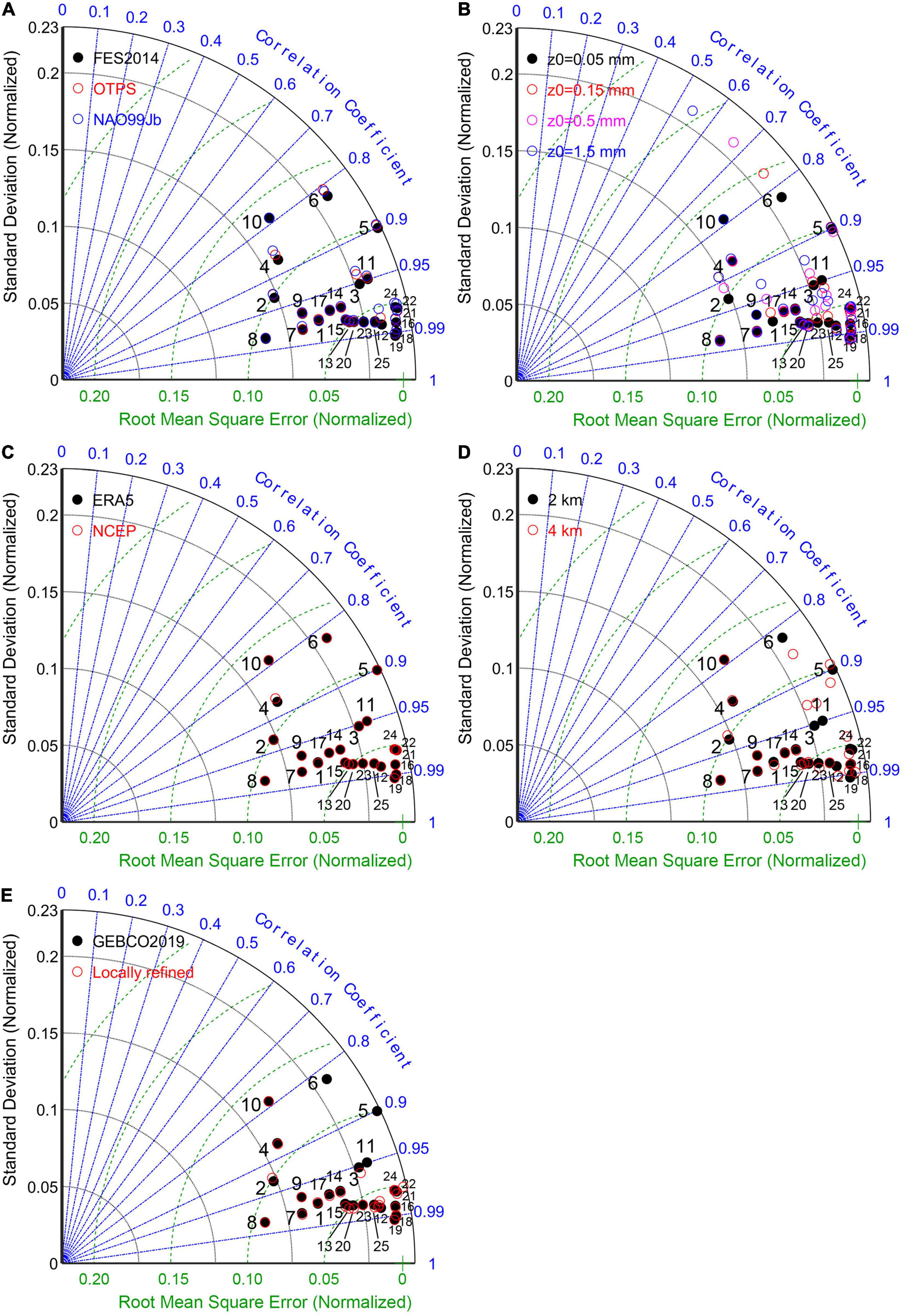
Figure 3. Taylor diagrams of the observed SSH at all tide gauges vs. simulations in all model scenarios of this study: (A) Baseline, Obd1, and OBd2, (B) Baseline, Z01, Z02, and Z03, (C) Baseline and Afd, (D) Baseline and Gr, (E) Baseline and Bd (Table 1). Distances from the lower left black origin marked by the y-axis and the black dotted arcs are the normalized standard deviations of the observational SSH. Distances from the green cross marked by the x-axis and the green dashed arcs are the RMSEs between the simulated and observational SSH. Blue lines indicate the correlation coefficients between the simulated and observational SSH. See Figure 1 for location of tide gauges.

Of all three tide models applied in this study, FES2014 seems to be superior to the others, as shown by higher CCs and lower RMSEs at most stations in the baseline scenario (Figure 3A). An exception is Station 21, where OTPS and NAO99Jb demonstrates better model performance (Figure 3A).

With different open boundary forcing, the M2 amplitude shows the following relationship at most tide gauges: OTPS > NAO99Jb > FES2014, except for Station 4, where FES2014 presents the largest M2 amplitude (Figure 4A). In contrast, the M2 phase is relatively insensitive to the open boundary setting (Figure 5A). FES2014 generally provides the M2 tide boundary better, as revealed by lower RMSEs (averaging 0.058 m in amplitude and 4.7° in phase) at tide gauges close to the open boundary (i.e., Stations 12, 4, 2, 8, 10, 9, 7, and 14). Based on the comparison between the Ob1 and baseline scenarios, OTPS produces stronger M2 tide than FES2014throughout the ECSs, particularly in the Taiwan Strait (Figure 6B). The open boundary induced discrepancies in the M2 phase are pronounced around Taiwan and in the Sea of Japan but are weakened as tides propagate into the semi-enclosed basin (Figure 6B).

FIGURE 4

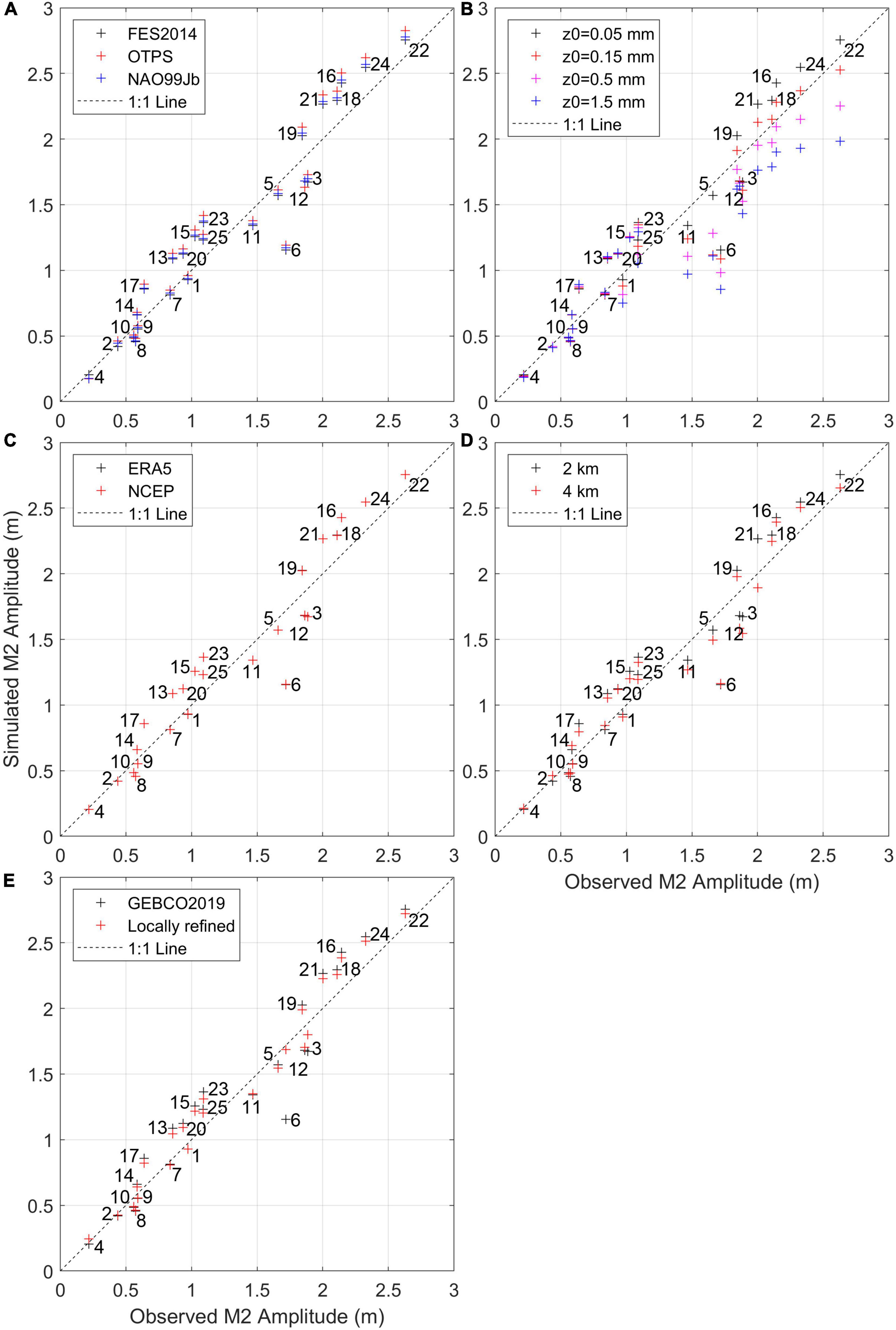
Figure 4. Comparison of the simulated vs. observed M2 amplitude in all model scenarios of this study: (A) Baseline, Obd1, and OBd2, (B) Baseline, Z01, Z02, and Z03, (C) Baseline and Afd, (D) Baseline and Gr, (E) Baseline and Bd (Table 1). Numbers in each panel indicate the tide gauges, the locations of which are shown in Figure 1.

FIGURE 5

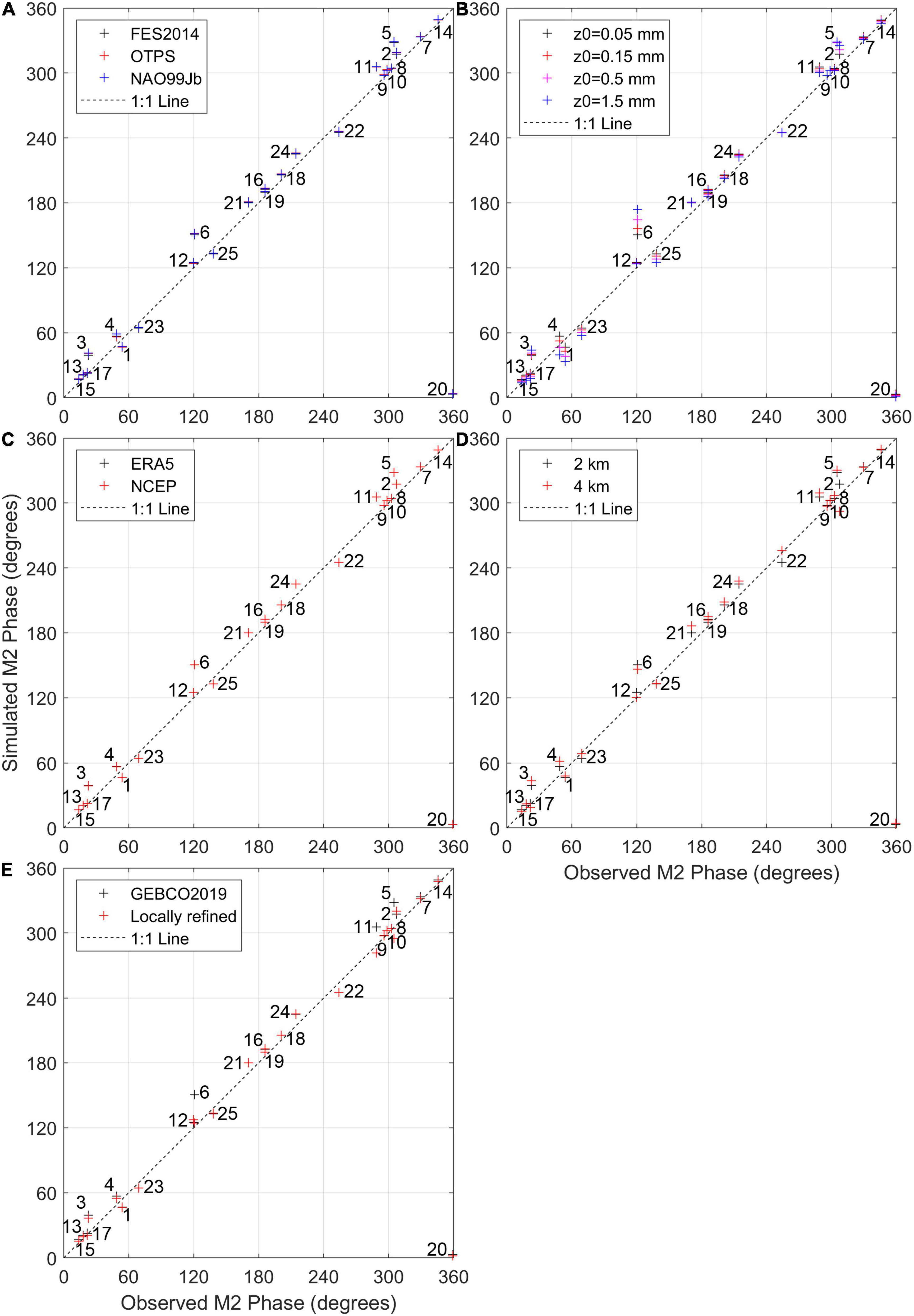
Figure 5. The same as Figure 4 but for the M2 phase. Model scenarios in each panel: (A) Baseline, Obd1, and OBd2, (B) Baseline, Z01, Z02, and Z03, (C) Baseline and Afd, (D) Baseline and Gr, (E) Baseline and Bd (Table 1).

FIGURE 6

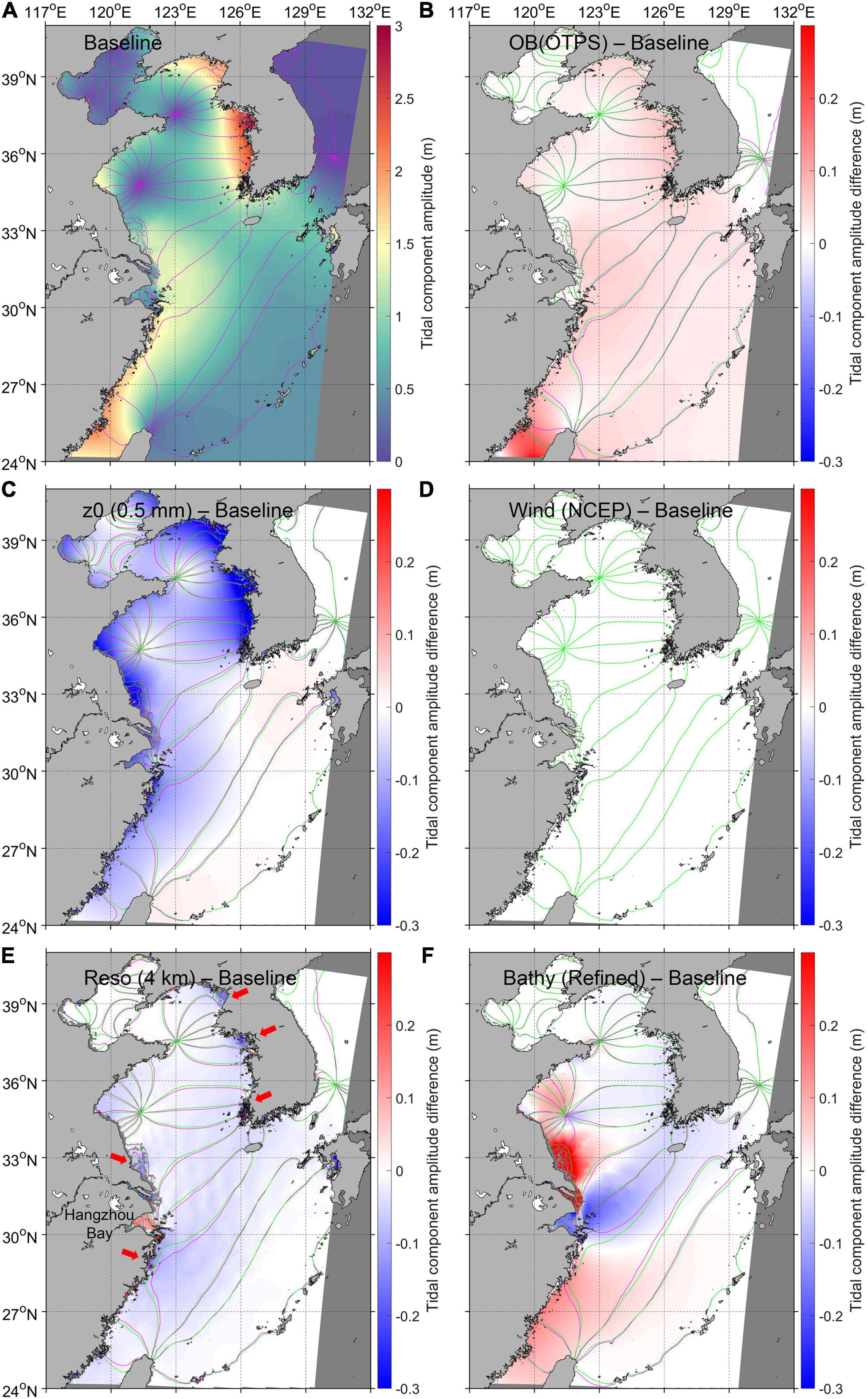
Figure 6. (A) The M2 cotidal graph of the baseline scenario and the difference between the (B) Obd1, (C) Z02, (D) Afd, (E) Gr, (F) Bd and baseline scenarios. In (B–F), the red or blue background colors indicate the difference in M2 amplitude, while the green and pink lines are the co-phase lines of the baseline and respective scenarios. See Table 1 for settings of scenarios.

Similar to M2, the K1 tide is stronger in the simulation with OTPS boundaries at all 25 tide gauges in the ECSs but weaker in the Sea of Japan, and the other two open boundary inputs tend to underestimate K1 (Figures 7B, 8A). Standard deviations of the K1 phase at the 25 tide gauges among the baseline, Ob1, and Ob2 scenarios (1.0°, 4.0 min) are about twice (four times) as much as that of the M2 phase (0.48°, 0.99 min) in terms of degrees (time), indicating a much larger inter-model difference (Figures 5A, 9A). At tide gauges close to open boundaries, OTPS and FES2014 simulate the K1 amplitude (RMSE = 0.0082 m) and phase (RMSE = 3.1°) better, respectively.

FIGURE 7

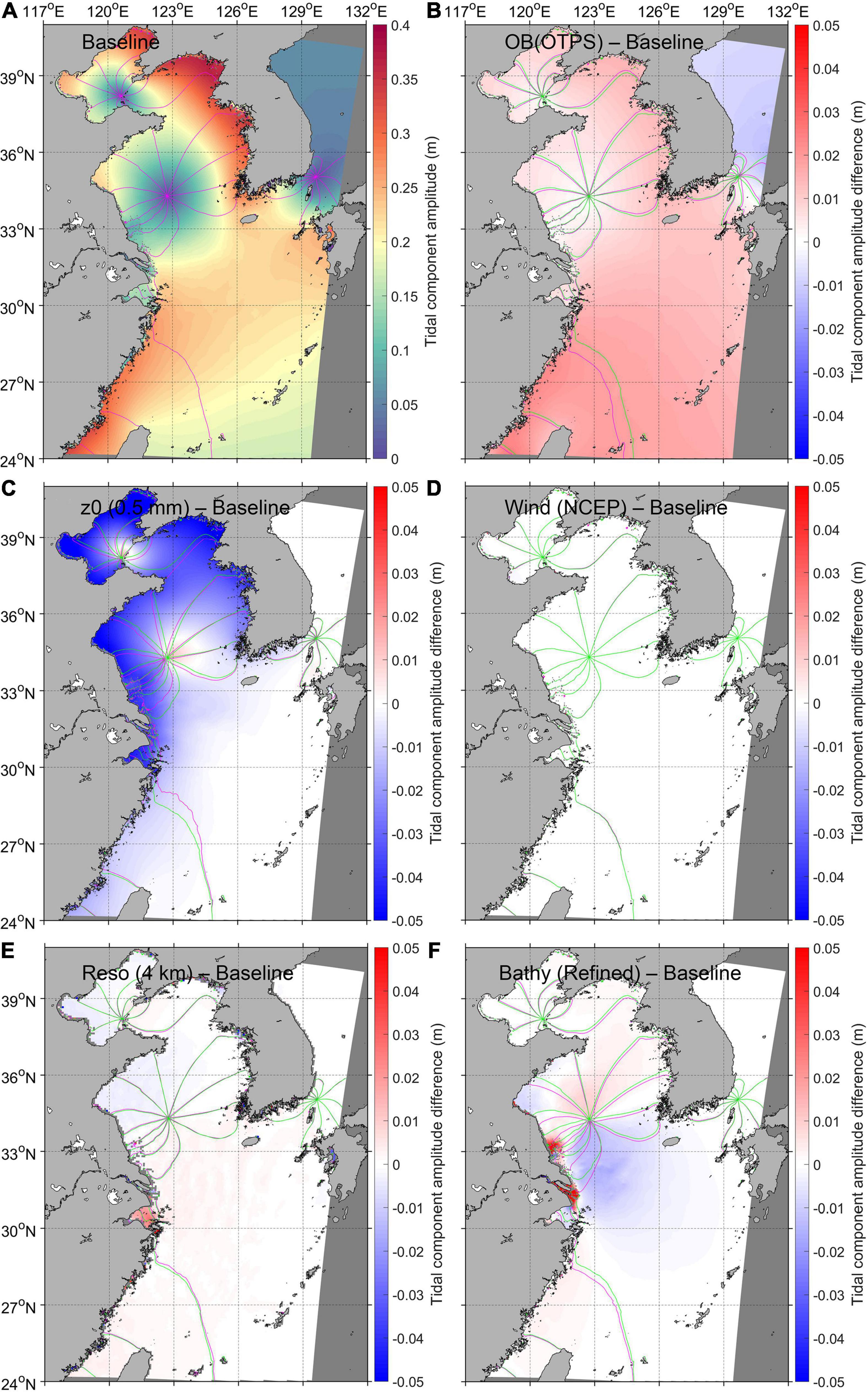
Figure 7. The same as Figure 6 but for the K1 tide. Model scenarios in each panel: (A) Baseline, (B) Obd1 – Baseline, (C) Z02 – Baseline, (D) Afd – Baseline, (E) Gr – Baseline, (F) Bd – Baseline (Table 1).

FIGURE 8

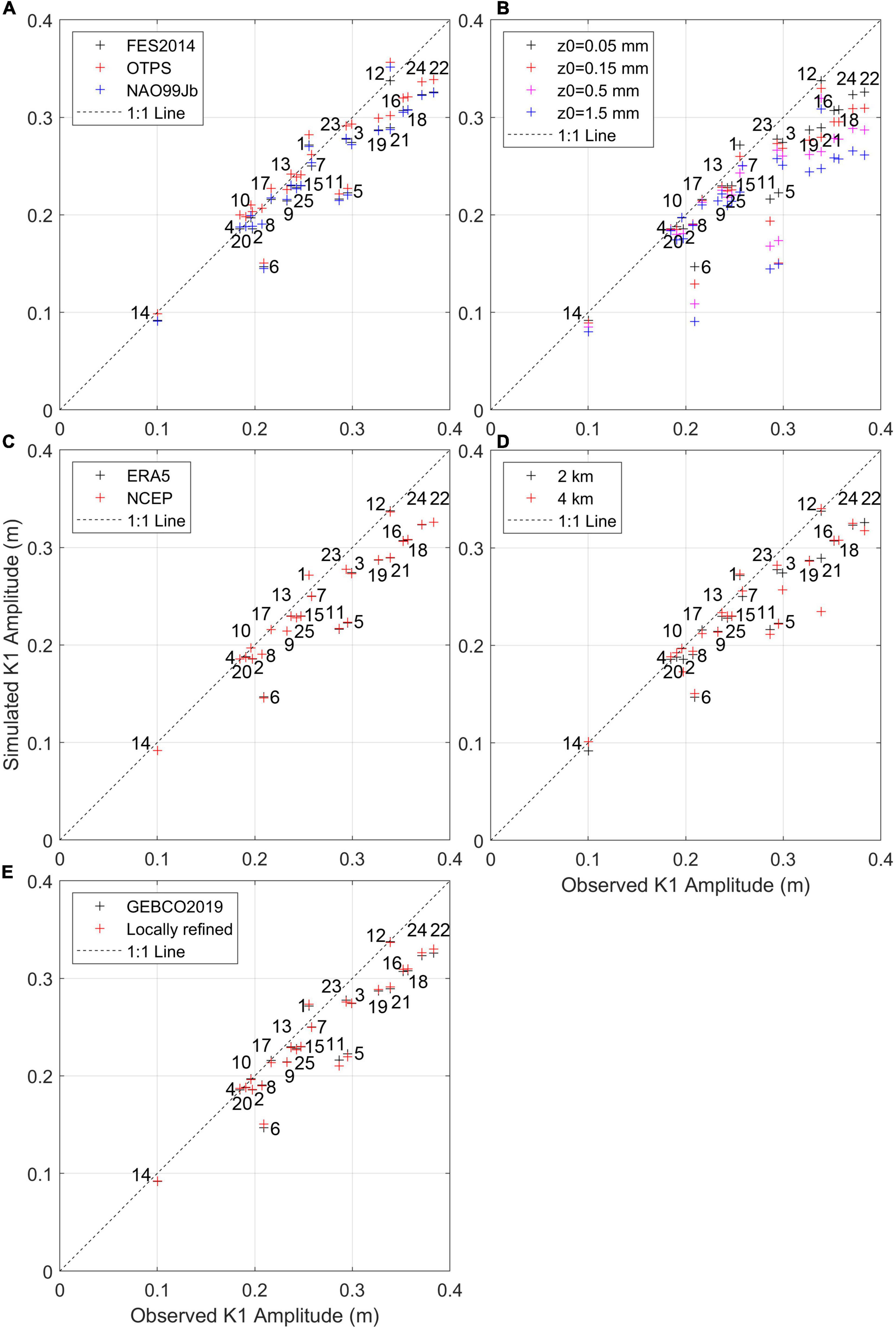
Figure 8. The same as Figure 4 but for the K1 amplitude. Model scenarios in each panel: (A) Baseline, Obd1, and OBd2, (B) Baseline, Z01, Z02, and Z03, (C) Baseline and Afd, (D) Baseline and Gr, (E) Baseline and Bd (Table 1).

FIGURE 9

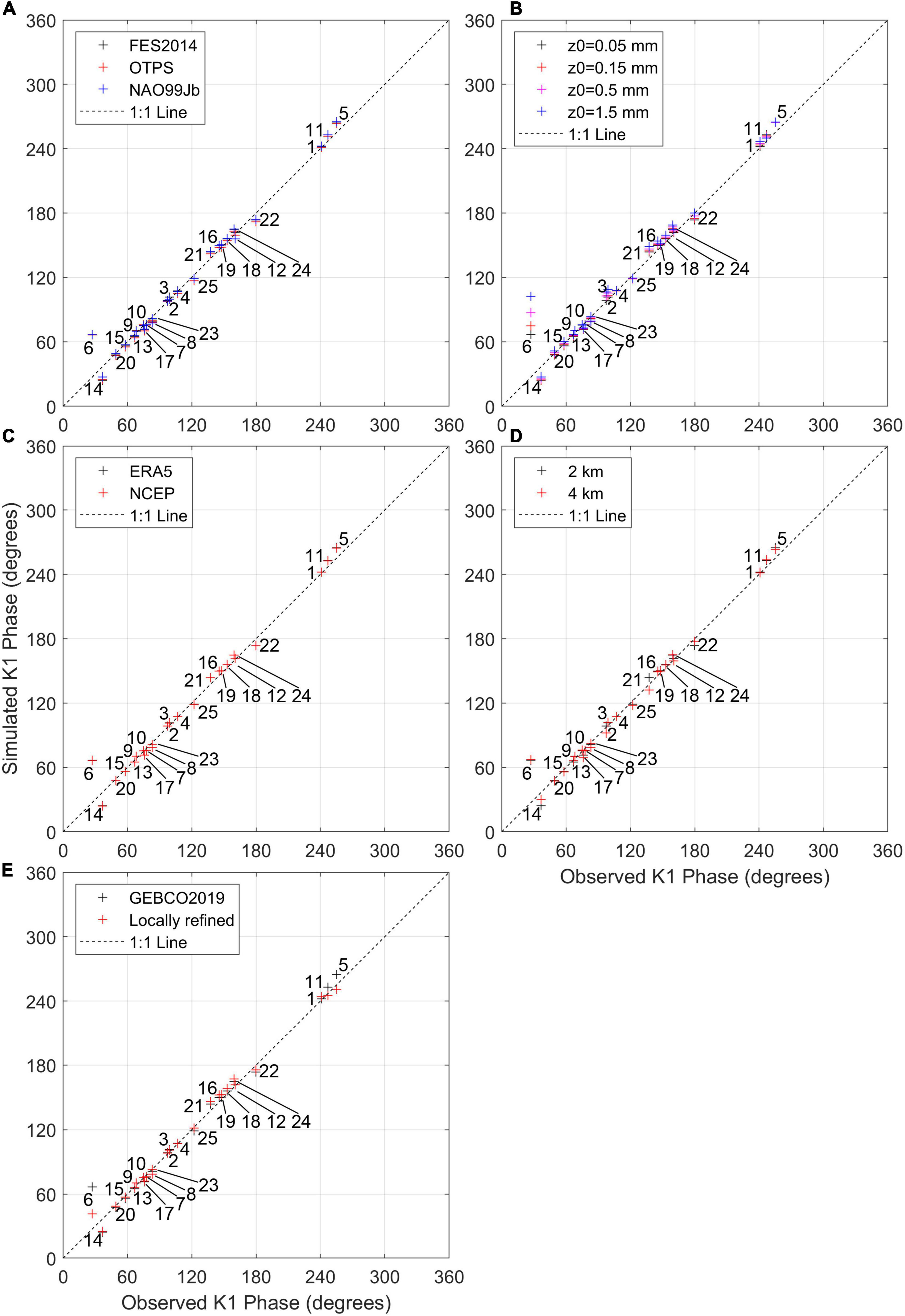
Figure 9. The same as Figure 4 but for the K1 phase. Model scenarios in each panel: (A) Baseline, Obd1, and OBd2, (B) Baseline, Z01, Z02, and Z03, (C) Baseline and Afd, (D) Baseline and Gr, (E) Baseline and Bd (Table 1).

To summarize, three tide models display some discrepancies in tidal elevation and main constituents at the open boundary, especially near Taiwan and in the Sea of Japan, which can radiate into the ECSs domain. Overall, FES2014 exhibits better agreements with the observed SSH and the M2 tide. Modelers of this region should notice that the inter-model discrepancies of the diurnal phase are greater than the semidiurnal.

Impacts of Bottom Roughness on Sea Surface Height and Tide Simulations

Considering a tidal Kelvin wave entering a rectangular semi-enclosed basin, Rienecker and Teubner (1980) and Pugh (1981) give an analytical solution that amphidromes in the northern hemisphere tend to shift left in the presence of friction. This phenomenon is reproduced by our model that the incoming Kelvin waves in the Yellow Sea are wider than the outgoing waves (Figures 6A, 7A). As a result of the increasing z₀ and friction, the amphidromes move further left relative to the incoming Kelvin waves (Figures 6C, 7C). Meanwhile, as bottom friction increases, the incoming tidal waves become faster compared to the exiting in an amphidromic system, which is illustrated by the decreased (increased) tidal phase on the right (left) side of the amphirdormes looking into the semi-enclosed basin (Figures 5B, 6C, 7C, 9B).

An intuitive result of increasing bottom roughness and frictional dissipation is the reduction of tidal amplitude in most of the ECSs, especially in shallow (< 100 m) coastal waters (Figures 6C, 7C). In addition, looking into the direction of tidal wave propagation, due to the left movement of amphidromes, some regions to the right are further away from the amphidromes, where the tidal amplitude increases slightly (Figures 4B, 6C, 7C).

Overall, the increased bottom roughness induces weakened tidal amplitude and shifted amphidromes, which results in various changes in SSH model skills depending on the location of tide gauges (Figure 3B). A low, intermediate, and high z₀ is favorable for lowering the SSH errors at Stations 6, 5, and 11, respectively (Figure 3B), although they are closely located (Figure 1).

Impacts of Atmospheric Data on Sea Surface Height and Tide Simulations

Over the episodic timescales (hours to days), discrepancies between the NCEP and ERA5 atmospheric forcing lead to uncertainties in SSH simulations. For instance, on 19 January 2019, the difference in wind speed can exceed 5 m/s (Figure 10A). The difference-induced wind stress curl creates a convergence/divergence zone in the East China/Yellow Sea and generates an instantaneous SSH difference up to 5 cm (Figure 10A). Likewise, in the Bohai Sea, the NCEP southerly winds are stronger than ERA5 southerlies, inducing a meridional SSH slope over 5 cm (Figure 10A). Differences of the two meteorological datasets are largest during storms. For example, the Super Typhoon Lekima is stronger in the NCEP reanalysis than ERA5, and the surge differs by ± 15 cm (Figures 10B–D).

FIGURE 10

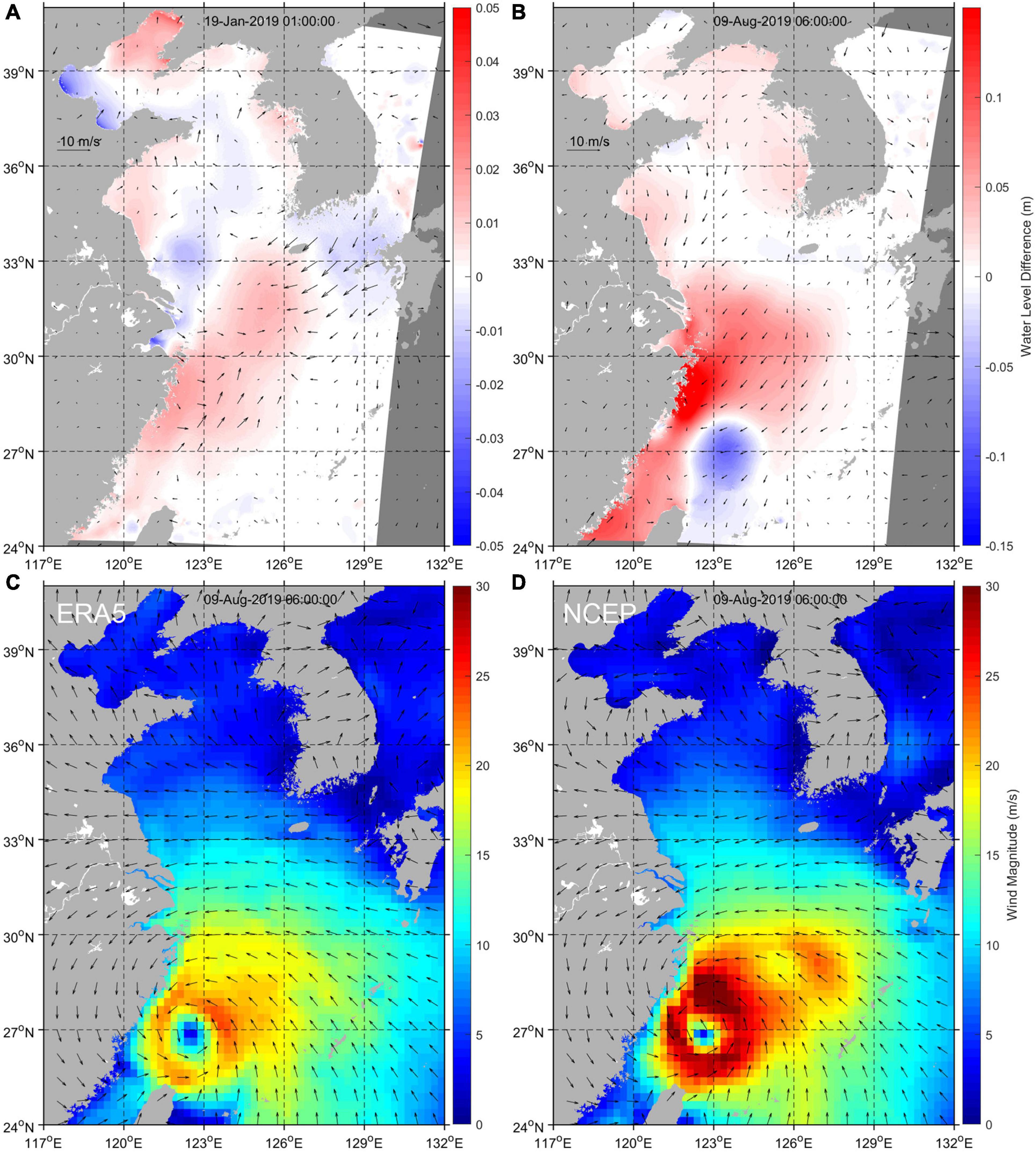
Figure 10. Differences in SSH (background color) and winds (arrows) at (A) 19 January 2019 1:00 and (B) 9 August 2019 6:00 calculated as the Afd (with NCEP forcing) minus the baseline (with ERA5 forcing) scenario. (C,D) Indicate the (C) ERA5 and (D) NCEP wind magnitude and direction at the same time as (B), right before landing of the Super Typhoon Lekima. Note that arrows in (C,D) only represent wind directions.

However, when it comes to the annual scale, the selection of atmospheric forcing exerts a minimal influence on the simulated SSH or tides in the ECSs, since the SSH model skills and tidal constituents extracted from 1-year data are mostly identical whether driven by ERA5 or NCEP data (Figures 3C, 4C, 5C, 6D, 7D, 8C, 9C). The SSH simulation is slightly better at Station 4 in the baseline scenario (Figure 3C).

Impacts of the Model Resolution on Sea Surface Height and Tide Simulations

When depicting the coastlines, the Cartesian mesh grid with a coarser resolution inevitably generates more and larger sawtooth-like land-water boundaries that impede the propagation of tidal waves. Thus, compared to the 2-km-resolution baseline run, a coarser (4 km) spatial resolution results in reduction in the M2 amplitude and retardation of the M2 waves (i.e., increased M2 phases) in most of the domain, especially in regions with complex coastlines and bathymetry (marked with red arrows in Figure 6E). In coastal regions like the Hangzhou Bay (Figure 6E), the landward narrowing is enhanced in the coarser grid so that local tides are further amplified (Figures 6E, 7E). Semi-diurnal tides with a shorter wavelength are more sensitive to model resolution than diurnal (Figures 6E, 7E).

With a coarser model grid, the average RMSE between the observed and simulated M2 amplitude decreases (from 0.164 to 0.153 m, Figure 4D), but that of the M2 phase increases (from 7.84° to 8.69°, Figure 5D). The K1 amplitude is better simulated in the 2-km-resolution (RMSE = 0.0265 m) than 4-km-resolution model (RMSE = 0.0294 m, Figure 8D), while the K1 phase is the opposite (RMSE lowers from 4.99° to 4.77° in the coarser-grid model, Figure 9D). Namely, a higher resolution (2 km vs. 4 km) does not seem to improve the tide simulation. However, the higher-resolution model performs better in modeling SSH at the majority of tide gauges, particularly where SSH is not well simulated (Figure 3D). For example, of all 15 tide gauges where RMSEs between simulated and observed SSH are over 0.05, most stations, except 1 and 6, show higher or equivalent model skills in a higher-resolution model (Figure 3D).

Impacts of Bathymetry Data on Sea Surface Height and Tide Simulations

When applying the refined bathymetry in the southern Yellow Sea (Figure 1), SSH simulation is greatly improved at the tide gauges covered by the new bathymetry (Stations 5, 6, and 11) and in surrounding regions (e.g., Stations 3 and most Korean stations) (Figure 3E). Errors of modeled M2 and K1 tides are prominently reduced throughout the ECSs (Figures 4E, 5E, 8E, 9E), largely accounting for the improvement in SSH simulation.

Bathymetry-induced changes in tides include the redistribution of amphidromes in the southern Yellow Sea and associated changes in tidal amplitude and phases (Figures 6F, 7F). The sand ridges and tidal channels between 31 and 34°N in the southwestern Yellow Sea are better depicted in the refined bathymetry (Figure 1), where changes in tides are most pronounced (Figures 6F, 7F). Impacts of the refined bathymetry reach as far as hundreds of kilometers away, such as the Taiwan Strait and South and West Coasts of the Korean Peninsula (Figure 6F). In comparison, the Bohai Sea to the north and deep regions close to the open boundary are less affected (Figures 6F, 7F).

Discussion

SSH and tide simulations have been a challenge in shelf and coastal seas (Wang et al., 2009; Zijl et al., 2013). In the ECSs, such applications start in the 1970s (e.g., An, 1977) and the modeling skill keeps improving in the last decades (Tang, 1988; Yanagi and Inoue, 1994; Guo and Yanagi, 1998; Kang et al., 1998; Shulman et al., 1998; Lee and Jung, 1999; Bao et al., 2001; Naimie et al., 2001; Lee et al., 2002; Xia et al., 2006; Yao et al., 2012; Ge et al., 2013; Su et al., 2015; Feng et al., 2019; Nguyen and Lee, 2020). Many of these studies tend to calibrate their models with the empirical tidal components rather than SSH. Our model skills of major tidal components are comparable to them (e.g., Ge et al., 2013; Lee et al., 2013; Nguyen and Lee, 2020), which also means that there is much room for improvement.

Uncertainty Sources in Sea Surface Height Simulations of the Eastern China Seas

In our case study of the ECSs, open boundary forcing, bottom roughness, atmospheric forcing, the model resolution, and bathymetry play different roles in SSH simulations. Of these uncertainty sources, atmospheric forcing appears to be the least important, partly because the meteorological it is sufficiently well reproduced by the reanalysis products of ERA5 and NCEP. Their differences and the induced episodic uncertainties of SSH are negligible on the annual scale (Figure 3C). In addition to scenarios presented in this study, by switching off river input, we examined the role of river discharge in SSH and tide simulations. It turns out that it has a trivial impact on the shelf sea, even smaller than meteorological forcing, which is consistent with the prior finding that river discharge can be neglected in such applications (Su et al., 2015).

In the baseline scenario, relative RMSEs between the simulated and observed SSH are over 7.5% at only five tide gauges, i.e., Stations 6 (0.126), 10 (0.125), 5 (0.105), 2 (0.091), and 4 (0.087), and CCs at these stations are below 0.95 (Figure 3). Among these five stations with worst simulated SSH, the locally refined bathymetry substantially improves the model skill of two inner stations, 5 (RMSE = 0.051, CC = 0.976) and 6 (RMSE = 0.041, CC = 0.984), but has little impact on the other three near the open boundary (Figure 3E). Of the three tide models used for open boundary inputs, while FES2014 is likely superior to the others, none is able to substantially reduce the SSH errors at these three stations (Figure 3A), neither is changing bottom roughness or grid resolution (Figures 3B,D). Hence, in terms of “fixing the shortest boards of a wooden barrel,” our results underline open boundary forcing as another key uncertainty source in SSH simulation of the ECSs in addition to bathymetry.

According to Zijl et al. (2013), the model resolution and shallow-water dynamics including tidal wave propagation and dissipation, rather than open boundary forcing, are key to the SSH simulation in the Northwest European Shelf and North Sea, a marginal sea similar to the ECSs in terms of the basin geometry, spatial scale, and tidal range. It is likely that the bathymetry and open boundary data are better measured and modeled in the Northwest European Shelf than the ECSs.

Uncertainty Sources in Tide Simulations of the Eastern China Seas

Uncertainties of the Amphidromic Points

As a dominant component in the SSH variations, tides in the semi-enclosed ECSs are featured by multiple amphidromic systems (Figures 6A, 7A) because of reflection of Kelvin waves (Taylor, 1920). Positions of amphidromes regulating the tidal amplitude and phases in the associated regions have been discussed in many tide simulation studies (e.g., Guo and Yanagi, 1998; Kang et al., 1998; Yao et al., 2012; Yao, 2016). Our results demonstrate that the amphidromic points are most sensitive to bathymetry and bottom roughness and relatively insensitive to the model resolution, open boundary forcing, and meteorological forcing (Figures 6, 7).

In addition to precisely delineating bathymetry and coastlines, adjusting local C_d conduces to accurately locating the amphidromes in tide simulations. Pugh (1981) derived that the amphidrome in a channel with constant depth h should displace from the centerline by $y = - \frac{\sqrt{g h} \cdot l n α}{2 f}$ in the northern hemisphere, where f is the Coriolis frequency, g is the gravitational acceleration, and α is the friction-induced attenuation ratio between the reflected and incident tidal waves. This analytical solution explains the wider (in the direction perpendicular to wave propagation) incidental waves than the reflected, as well as the further left displacement of amphidromes relative to the wave propagation direction induced by enhanced friction (Figures 6C, 7C). By integrating empirical tide data, Fang et al. (2004) detect two M2 amphidromes close to the land-sea boundary in the northern and southwestern Bohai Sea, respectively, which appear further landwards (i.e., degenerate amphidromes) in Guo and Yanagi (1998) and Varlamov et al. (2015), and our study, and further seawards in Ogura (1936), Yao et al. (2012), and Ge et al. (2013), etc. These variations in amphidromic points indicate relatively strong or weak friction in the Bohai Sea, respectively, for which coastal morphological changes, different bathymetry datasets, and discrepancies in C_d parameterization are potential causes.

Uncertainties of the Tidal Amplitude

The modeled tidal amplitude in the ECSs is a combined result of all tested factors except meteorological forcing (Figures 6, 7). Of these four factors, open boundary forcing and bottom roughness have specific and predictable effect on the tidal amplitude throughout the domain. Specifically, a large z₀ and low tidal amplitude of a certain constituent (e.g., M2) at the open boundaries reduce the M2 amplitude in the entire ECSs (Figures 6, 7). In contrast, variations in bathymetry and grid resolutions (i.e., coastlines) have relatively strong but non-uniform effects on tidal amplitude in the basin, especially in shallow waters (Figures 6, 7).

It is inferred from our findings that overestimated (underestimated) incoming tides from the open boundaries combined with overestimated (underestimated) C_d may lead to similar simulated tidal amplitude that matches the observation. Yet, the aforementioned combination of open boundary inputs and C_d may not be realistic. This has important implications for understanding the wide selection of z₀, C_d, and open boundary forcing in previous ECSs tide models. For instance, C_d in our baseline scenario (< 0.001 on average, Figure 2) is similar to that applied by Feng et al. (2019), in the lower range of that assimilated by Lu and Zhang (2006, 0.0001–0.003), and significantly lower compared to many ECSs models (e.g., 0.0035, Lee and Jung, 1999; 0.0015, Bao et al., 2001; 0.0015–0.00175, Hu et al., 2010; 0.002–0.0035, Nguyen and Lee, 2020). With a relatively low bottom roughness, our study finds the FES2014 data with relatively weak semidiurnal tides preferable as open boundary forcing. In contrast, Nguyen and Lee (2020) apply relatively strong bottom friction as well as semidiurnal tides (NAO99Jb) in their selected case. This phenomenon is named as equifinality in sediment models, which affects the predictive capacity of models (van Maren and Cronin, 2016).

Uncertainties of the Tidal Phase

Bathymetry, bottom friction, and the grid resolution have dominant impacts on tidal phases in the ECSs, while differences in open boundary tidal phases gradually diminish as tidal propagation into shallow waters (Figures 6, 7). Changes in tidal phases induced by bathymetry and bottom friction are mostly associated with redistribution of amphidromes discussed in sections “Impacts of Bottom Roughness on Sea Surface Height and Tide Simulations,” “Impacts of Bathymetry Data on Sea Surface Height and Tide Simulations,” and “Uncertainties of the Amphidromic Points.” In contrast, variations in model resolutions do not lead to marked shift of amphidromes but affect the delineation of coastlines and shallow-water tidal deformation (e.g., damping, convergence, and reflection). The resulting uncertainties in tidal phases are notable in regions with complicated or abruptly changing coastlines (Figure 6E).

It is noteworthy that increasing bottom friction and using a coarser model grid have complementary effects on the M2 phase on the West Coast of Korea (Figures 6C,E). Specifically, if model calibration is only concerned in this region, uncertainties from an insufficient grid resolution can be offset by adding bottom friction basin-wide, making them difficult to discern and eliminate.

Recommendations for Future Endeavors

Prior studies attempting to decompose and reduce uncertainties in modeled SSH and tides in regional seas highlight the importance of open boundary forcing (Abdennadher and Boukthir, 2006; Yao et al., 2012), bottom friction (Lu and Zhang, 2006; Zijl et al., 2013; Nguyen and Lee, 2020), model resolutions (Falcão et al., 2013; Zijl et al., 2013), or bathymetry data (Lee et al., 2013; Quaresma and Pichon, 2013) as the main uncertainty source. After examining their influences, we have the following suggestions for such attempts in the ECSs and other regional seas.

Acquiring the realistic bathymetry is the priority of all efforts. Of all the scenarios in our study, locally refined bathymetry reduces errors in SSH and tides to the largest extent. As implied by our results (e.g., section “Uncertainties of the Tidal Amplitude”), adjusting other model inputs or parameters with inadequately accurate bathymetry runs the risk of introducing unrealistic processes or overcorrecting the bathymetry-induced errors. However, open-access bathymetry datasets for the ECSs are limited except for some global ones such as GEBCO and ETOP (by the National Geophysical Data Center). Extensive measurements of shelf and coastal bathymetry, as well as publicizing them are as important, if not more so, than developing high-resolution models with fine-tuning parameters.

With accurate bathymetry and coastline data, the next suggested practice is to find the optimal open boundary input before running any sensitive tests of model parameters. For example, tuning z₀ with biased boundary forcing likely produces additional errors in the simulated tides (section “Uncertainties of the Tidal Amplitude”). Boundary forcing can be selected by comparing candidates with observations near open boundaries, in our case, Stations 12, 4, 2, 8, 10, 9, 7, and 14. In such attempts of our study, none of the three candidates seems completely superior to the others. FES2014 simulates semidiurnal tides of these stations with fewer deviations, especially around the Taiwan Strait (Figure 4A), but largely underestimates diurnal tides along the Ryukyu Islands (Figure 8A). In addition to seeking better alternatives, Yao (2016) suggests correcting the existing tide model output using observational data near the boundaries, which, as a potential solution, still needs an algorithm to fill the spatial gaps between observations.

Another uncertainty source, bottom roughness, should be adjusted after bathymetry and open boundary forcing. The best practice would be to set the z₀ or C_d range based on measurements in the bottom boundary layer (e.g., velocity at 1 m above the seabed, Soulsby, 1983) and the sediment grainsize map (Thiébot et al., 2020b). In shelf seas such as the Northwest European Shelf and ECSs, sediment grainsize is mostly mapped (Zeng et al., 2015; Wilson et al., 2018; Mi et al., 2020). However, sediment mixture composition, morphology of seabed ripples, and even near-bottom suspended sediments change the z₀ magnitude (Soulsby, 1983). Given that these data or bottom boundary layer measurements are sparse or unavailable, many regional models tune z₀ or C_d for optimal matches with observations, some using data assimilation (Lu and Zhang, 2006; Nguyen and Lee, 2020). While it may be effective, caution needs to be used for equifinality, i.e., different combinations of model parameters/settings may produce similar model performance. Hence, the large C_d range in prior ECSs studies (0.0001–0.0035, section “Uncertainties of the Tidal Amplitude”) generally reflects the inter-model uncertainties, which should be eliminated by optimized z₀ or C_d estimation referring to in situ measurements, as well as improved bathymetry data, boundary forcing, and other model settings.

Furthermore, increasing the grid resolution may not be an effective solution to all biases. A higher grid resolution results in improved model skills in many global (Lyard et al., 2006, 2021; Zu et al., 2008; Stammer et al., 2014) and regional (Lefevre et al., 2000; Zijl et al., 2013) tide models, as well as SSH in our study. However, increasing the grid resolution to a certain extent, 2–1 km in the study by Lee et al. (2013) and 4–2 km in our study, does not significantly improve the modeled tides, since the grid resolution may not be the largest uncertainty source.

Last but not least, when conducting model calibration, the ECSs, or other shelf seas, should be considered as an entire system. According to our results, local adjustment in model settings (bathymetry, open boundaries, etc.) has far-reaching influences on regions hundreds of kilometers away, especially those within the same amphidromic system. Moreover, focusing on part of an amphidromic system is unfavorable for discerning opposite deviations caused by different factors (section “Uncertainties of the Tidal Phase”). A thorough model assessment should include observational data not only in the area of interest (e.g., Feng et al., 2019; Nguyen and Lee, 2020) but all around the basin. While the observed SSH collected in this study lasting several decades satisfies this need, tidal current data of sufficient spatial coverage and temporal span are mostly unavailable in the ECSs. A similar modeling assessment of tidal current requires increasingly extensive flow measurements and an updated data-sharing agreement involving several countries around the ECSs. Additionally, given the SSH seasonal variation, we recommend using at least 12-month time series for validation of tidal harmonics.

Conclusion

SSH and tide simulations are relatively inaccurate in shelf seas. Even though tide simulations in the ECSs have been reported for decades, it remains one of the shelf seas with highest inter-model standard deviations (Stammer et al., 2014). Rather than presenting a perfect model with fewest errors, our study explores potential uncertainty sources and their effects on SSH and tide modeling.

Our results indicate that SSH and tide modeling accuracy is primarily constrained by bathymetry data, and regionally refined bathymetry reduces biases locally as well as hundreds of kilometers away. Open boundary forcing provided by FES2014, OTPS, or NAO99Jb is associated with large uncertainties, especially in shallow waters near Taiwan and Sea of Japan, which can penetrate into the entire ECSs. FES2014 simulates SSH and semidiurnal tides better but extensively underestimates diurnal tides. Besides adding frictional dissipation, increasing z₀ and C_d affects the amphidromic system by amplifying the relative strength of incoming to exiting Kelvin waves, with shifted amphidromes and corresponding tidal phases. Impacts of adjusting the grid resolution are mainly revealed in the nearshore waters with complicated coastlines. A higher resolution (2 km vs. 4 km) does not improve the overall model skill of tides but that of SSH. Using different meteorological forcing data produces SSH uncertainties of mostly a few centimeters over timescales of hours to days, which is insignificant on the annual scale.

In addition to the individual impacts of the five examined uncertainty sources, our study highlights their combined effects and the possible equifinal model settings. “All models are wrong but some are useful” (Box, 1976). Factors that have opposing effects on SSH, tidal amplitude, or tidal phases may counteract their respective biases, diminish the simulation deviations in part of or the entire domain, but make the model less “useful,” i.e., reduce predictive capability of the model.

As Lyard et al. (2006) claim, data assimilation cannot be the ultimate answer to a better tide model or replace the efforts of improving the simulation of tidal dynamics. Our non-assimilative findings offer insights into developing a more “useful,” or realistic, ECSs model, which should be applicable to modeling other regional seas as well as designing data assimilation strategies.

Data Availability Statement

The raw data supporting the conclusions of this article will be made available by the authors, without undue reservation.

Author Contributions

LJ and XC designed and conducted the modeling study. LJ, XL, and WX performed data analysis. PY prepared the locally refined bathymetry. LJ drafted the manuscript. All authors edited the manuscript.

Funding

This research was funded by the National Key Research and Development Program of China (2018YFD0900906 and 2020YFD0900701), the National Natural Science Foundation of China (42106027), and the Natural Science Foundation of Jiangsu Province (BK20200517). The work was carried out at National Supercomputer Center in Tianjin, and this research was supported by TianHe Qingsuo Project special fund project in the field of climate, meteorology and ocean.

Conflict of Interest

The authors declare that the research was conducted in the absence of any commercial or financial relationships that could be construed as a potential conflict of interest.

Publisher’s Note

All claims expressed in this article are solely those of the authors and do not necessarily represent those of their affiliated organizations, or those of the publisher, the editors and the reviewers. Any product that may be evaluated in this article, or claim that may be made by its manufacturer, is not guaranteed or endorsed by the publisher.

Acknowledgments

We appreciate the constructive comments of the editor and three reviewers.

Footnotes

References

Abdennadher, J., and Boukthir, M. (2006). Numerical simulation of the barotropic tides in the Tunisian shelf and the strait of Sicily. J. Mar. Syst. 63, 162–182. doi: 10.1016/j.jmarsys.2006.07.001