Surface Warming Slowdown With Continued Subsurface Warming in the East Sea (Japan Sea) Over Recent Decades (2000–2014)

The long-term surface warming trend in the East Sea (Japan Sea; ES hereafter) stalled from 2000 to 2014 (−0.05°C yr⁻¹, surface warming slowdown), while the subsurface (100–300°m) warming trend continued (+0.03°C yr⁻¹). To address the processes underlying these contrasting trends in surface and subsurface temperature change, the trends in sea-level anomaly, isopycnal depth, and wind pattern were analyzed using monthly mean ocean reanalysis system 4 (ORAS4) data. During this period, the strengthened northwesterly/northerly wind in the central part of ES is supposed to contribute to a negative (positive) wind stress curl to its west (east), corresponding to an anticyclonic (cyclonic) circulation in the west (east). Furthermore, the induced negative wind stress in the west appears to enhance the northward penetration of East Korean Warm Current (EKWC), the slowdown in its eastward meandering around 38° N from the Korea coast, resulting in warm water accumulation in the west with peak warm anomaly at relatively greater depth compared to peak cold anomaly in the east. Overall, these wind-driven changes in transport from west to east, wind stress curl induced horizontal divergence (convergence) and the associated upwelling (downwelling), causes surface warming to slow and subsurface warming to persist during 2000 to 2014.

Introduction

During the global warming hiatus period from 1998 to 2013 (IPCC, 2013, 2014; England et al., 2014), the surface warming trend decreased from 0.12^°C yr⁻¹ to 0.05^°C yr⁻¹; however, the heat content below the sea surface continued to increase, contrary to the pause in surface warming. For this reason, this period was later redefined as “global surface warming slowdown” (Yan et al., 2016; Han and Yan, 2018). Although many studies have been conducted to understand the surface warming slowdown processes on a global scale [e.g., Pacific Ocean (England et al., 2014; Kosaka and Xie, 2016); Indian Ocean (Lee et al., 2015); Atlantic Ocean (Levitus et al., 2012; Balmaseda et al., 2013; Chen and Tung, 2014); Southern Ocean (Lyman et al., 2010; Purkey and Johnson, 2010)], less research has been conducted on marginal seas despite the physical phenomena in marginal seas being active and responding rapidly to environmental change (Schroeder et al., 2017). Thus, the mechanism by which heat redistribution proceeds in regional seas should be understood by analyzing multiple forcing mechanisms (i.e., ocean circulation, wind stress, and large-scale climate variability; Liao et al., 2015). Therefore, we targeted the East Sea (Japan Sea; ES), which has various oceanic features (oceanic eddies, subpolar front, deep-water formation, etc.) but has a relatively short ventilation period, to investigate the surface warming slowdown (Gamo, 1999).

The ES is a semi-enclosed deep marginal sea connected to the Pacific through narrow and shallow straits, with the lowest deep-water temperature and highest deep-water dissolved oxygen in the Pacific. Moreover, it has high warming rates among all oceans worldwide and is significantly affected by global warming trend (Kim et al., 2001; Talley et al., 2006; Belkin, 2009; Gamo, 2011). Regarding subsurface water property changes, Nam et al. (2016) demonstrated that decadal changes in intermediate water relates to significant changes in the water formation, ventilation, and subduction processes in response to the surface atmospheric and oceanic conditions. Furthermore, decadal changes in the sea’s meridional overturning circulation shifting from/to one-cell to/from two-cell structures have recently been discovered (Han et al., 2020). The bottom water formation in ES has been enhanced since 2000, which indicates water formation and ventilation processes can provide significant climatic implication (Yoon et al., 2018).

Thus, it is crucial to understand how the warming slowdown has proceeded in the ES from the sea surface to the subsurface. The long-term global warming trend and climate patterns are well-reflected in the physical environments of the ES (Gordon and Giulivi, 2004; Lee et al., 2009; Lee and Park, 2019). Majority of studies on the variability of climate patterns affecting the ES have usually been based on the Siberian High (SH) and Monsoon (Jeong and Park, 2017; Gallagher et al., 2018). However, these studies have discussed the processes focused on conventional surface warming in the ES affected by the global warming trend. Therefore, this study aimed to determine whether the surface warming slowdown existed as opposed to the continued warming trend and clarify how the surface warming slowdown was induced in the ES.

Data and Methods

To investigate the surface warming slowdown in the ES, monthly ocean reanalysis system 4 (ORAS4) temperature data from the European Center for Medium-Range Weather Forecasts (ECMWF) is used. The ORAS4 sea level anomaly (SLA) and meridional and zonal current speeds (u, v) are also used for further wind-driven circulations from 1980 to 2017. The ORAS4 data with 1 spatial resolution is interpolated to 0.25°. We evaluated ORAS4 data quality using in situ measurements from CORIOLIS¹ and additional reanalysis datasets: GLORYS2, C-GLORS05, and ORAS5. All data show very similar trends (not shown), and we choose ORAS4 as it has a long temporal coverage and appropriate spatial resolution. The wind stress and wind stress curl were calculated using the monthly ERA-Interim surface wind (10 m) data provided by the ECMWF.

Ensemble empirical mode decomposition (EEMD) was used to investigate the decadal to multi-decadal variability of the sea surface temperature anomaly (SSTA), SLA, and wind stress curl. The EEMD method was developed by Wu and Huang (2009), which separates signals into intrinsic mode functions (IMFs) at different time scales. The decomposing process is done by identifying all the local maximum and minimum envelopes from the data and then fitting the adjacent extreme envelopes to the cubic spline. To derive the first IMF, connect all the local maxima and minima of the data with a cubic spline as the upper and lower envelope. The second IMF is sifted by repeating the same process above after subtracting the first IMF signal from the original data. The IMFs are extracted until the remaining oscillation has no time-frequency signal, and the remaining oscillation becomes a residual mode. Eventually, each IMF has its own time signal from high frequency to low frequency. Each variable for the whole study period (1980–2017) was decomposed into the eight IMFs and the monotonic residual. The 7–8th IMFs with a period of more than 10-years and secular trend (residual mode) were combined to analyze the multi-decadal variability from the time-series data. The significance of each IMF was determined using a spread function. In this study, only an IMF with a confidence level of 95% or higher was used.

In addition, the ocean heat content (OHC) was calculated and quantified. The SLA contains the total water column changes, including non-steric and steric signals. Thus, the SLA-based OHC was estimated instead of the temperature-based OHC calculation to separate the steric and non-steric components, enabling us to understand their contribution to OHC. Furthermore, because the SLA-based OHC above 300 m in the ES is coherent with the temperature-based OHC (not shown), the OHC of the ES can be calculated based on the SLA. The OHC derived from the SLA (Gill and Niller, 1973; Chambers et al., 1997; Wang and Koblinsky, 1997) is given by Eq. (1):

${\mathbf{\text{H}}}_{\mathit{SLA}}^{{}^{\prime }}=\frac{\mathrm{\rho }{\mathbf{\text{C}}}_{\mathbf{p}}}{{\mathrm{\alpha }}_{\mathbf{T}}}\mathit{\text{SLA}}(1)$

where ${\mathbf{\text{H}}}_{\mathit{SLA}}^{{}^{\prime }}$ is the heat content anomaly derived from the SLA, and the prime (′) symbol represents the anomaly. Here, ρ is the ocean density, C_p is the specific heat of seawater, and α_T is the thermal expansion coefficient. The constants in Eq. (1) are defined as ρ = 1,027kgm−³ and C_p = 4,000Jkg⁻¹K−¹ (Gill and Niller, 1973). The SLA in the Eq. (1) can further expand into thermal expansion effects, salinity effects, wind stress curl forcing, and waves, respectively (Eq. 2). Here, the thermal expansion and salt contraction effects are steric components, and wind stress curl forcing and wave terms are considered to have a non-steric effect on the SLA variation. Therefore, the change in SLA due to the steric effect can be expressed by Eq. (3), and we can obtain the OHC value by considering only the steric effect (Eq. 4) using steric height (SLA_Steric) following Eq. (1).

$\mathit{\text{SLA}}={\mathbf{\text{h}}}_{\mathit{\text{Thermal}}}^{{}^{\prime }}+{\mathbf{\text{h}}}_{\mathit{Salinity}}^{{}^{\prime }}+{\mathbf{\text{h}}}_{\mathit{Wind}}^{{}^{\prime }}+{\mathbf{\text{h}}}_{\mathit{Wave}}^{{}^{\prime }}(2)$

${\mathit{\text{SLA}}}_{\mathit{Steric}}={\mathbf{\text{h}}}_{\mathit{Thermal}}^{{}^{\prime }}+{\mathbf{\text{h}}}_{\mathit{Salinity}}^{{}^{\prime }}(3)$

${\mathbf{\text{H}}}_{\mathit{Steric}}^{{}^{\prime }}=\frac{\mathrm{\rho }{\mathbf{\text{C}}}_{\mathbf{p}}}{{\mathrm{\alpha }}_{\mathbf{T}}}{\mathit{\text{SLA}}}_{\mathit{Steric}}(4)$

To evaluate the variation in OHC due to heat redistribution through advection (i.e., non-steric effect), the steric effect (${\mathbf{\text{H}}}_{\mathit{Steric}}^{{}^{\prime }}$) is subtracted from the total OHC (${\mathbf{\text{H}}}_{\mathit{SLA}}^{{}^{\prime }})$ as in Eq. (5):

${\mathbf{\text{H}}}_{\mathit{Nonsteric}}^{{}^{\prime }}={\mathbf{\text{H}}}_{\mathit{SLA}}^{{}^{\prime }}-{\mathbf{\text{H}}}_{\mathit{Steric}}^{{}^{\prime }}(5)$

It’s important to note that, in the long-term and monthly data analysis, the SLA variation due to waves (${\mathbf{\text{h}}}_{\mathit{Wave}}^{{}^{\prime }}$) is very small and can be negligible. Thus, the OHC variation due to non-steric effects is almost regarded as variation by wind stress curl (${\mathbf{\text{h}}}_{\mathit{Wind}}^{{}^{\prime }}$) alone.

Results and Discussion

Surface Warming Slowdown Signal

To investigate the overall warming trend, the time series of the SSTA averaged over the entire ES was analyzed from 1980 to 2017. In Figure 1A, the SSTA continued to increase until about 2000, and the increasing trend subsequently slowed down during the period from 2000 to 2014, yielding the rate of SSTA change from 0.07°C yr−¹ to -0.02°C yr⁻¹. The temperature time series of the decadal time scale derived from EEMD also reveals a decrease in the warming trend between 2000 and 2014, as shown by the blue line in Figure 1A. Considering that the increasing trend of the global mean SSTA changed from 0.12°C yr⁻¹ to 0.05°C yr⁻¹ (IPCC, 2014) during the period from 2000 to 2014, the trend changes in the ES (declining by 0.09°C yr⁻¹) is similar to that of the global trend (declining by 0.07°C yr⁻¹). Therefore, this period was defined as the surface warming slowdown (SWS) period in the ES, and that before the SWS period (from 1985 to 1999) was defined as the surface warming (SW) period for comparison (Figure 1A). The difference in the long-term surface warming trend between the two defined periods shows a declining tendency in the overall ES, indicating that the surface warming slowed during the SWS period.

FIGURE 1

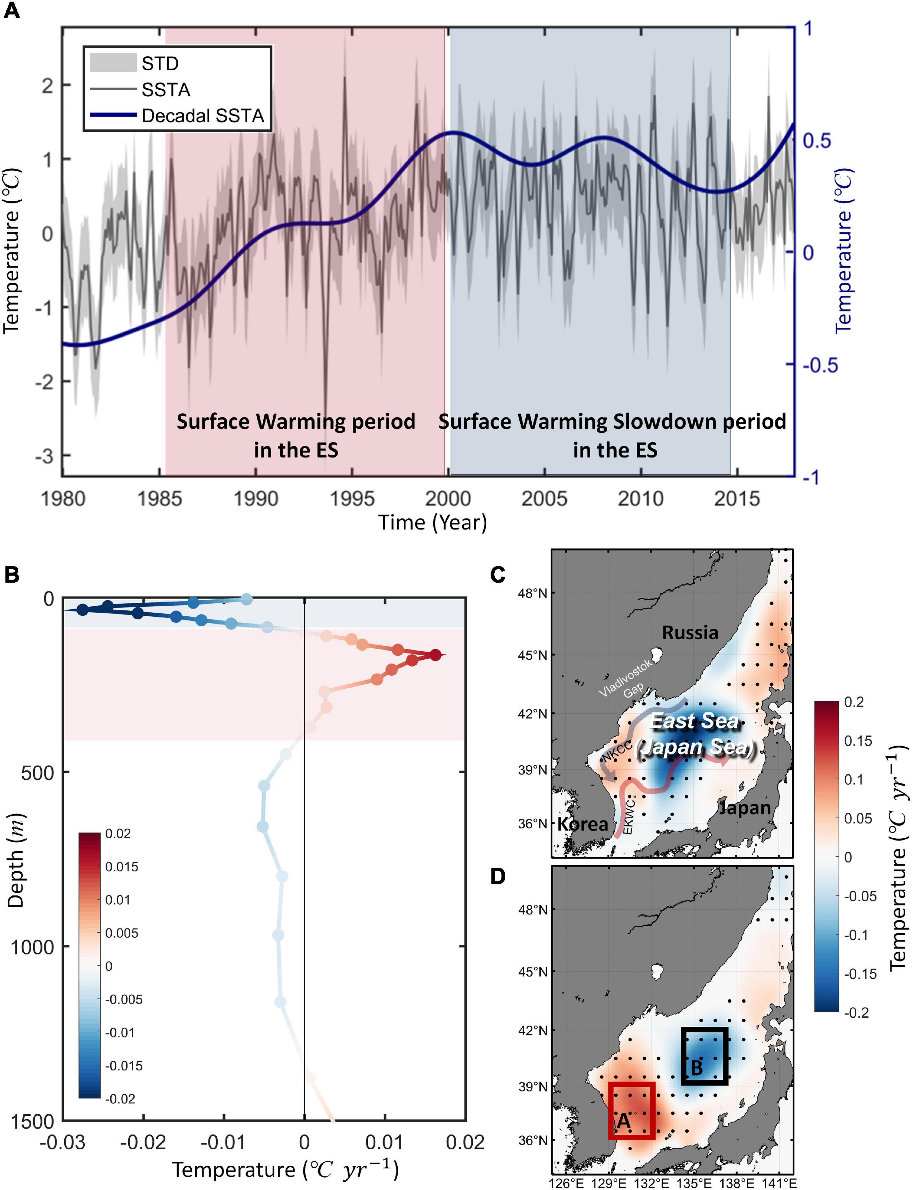
Figure 1. (A) Timeseries of sea surface temperature anomaly (SSTA) in the ES (black line) and its decadal mode (blue line) highlighting periods of surface warming (red shaded) and surface warming slowdown (blue shaded). Shading with gray lines indicates the standard deviation of each month for the SSTA. (B) Vertical profile of long-term trend in monthly mean temperature anomaly from 2000 to 2014 at the upper 1,500 m of the ES, indicating cooling and warming trends at the upper 100 m (blue shaded) and 100–300 m (red shaded), respectively. The vertical black line in panel (B) shows where the trend is zero. Spatial distribution of the temperature trend (C) for the upper 100 m of the ES and (D) depths from 100 to 300 m during the SWS period. The red and gray lines show the East Korea Warm Current (EKWC) and the North Korea Cold Current (NKCC), respectively (C). The red and black boxes indicate Regions A and B, respectively (D). Black dots in panels (C,D) indicate where the trends are significant at the 95% confidence level.

The declining tendency of the surface warming trend was compared with that of the trend in subsurface temperature at depths during the SWS period (Figure 1B). During the SWS period, the subsurface temperature in the upper 100 m showed a declining tendency of the warming trend, same as in the case of the SSTA. At depths between 100 and 300 m (intermediate layer), however, the trend in subsurface temperature significantly increased during the SWS period with a maximum increase rate of approximately 0.02°C yr⁻¹ at a depth of 200 m (Figure 1B). The spatial pattern of the temperature trend for the upper 100 m shows a strong declining trend in the central ES during the SWS period (Figure 1C). In the case of the intermediate layer (100–300 m), a distinct increase in the temperature trend was found in the southwestern ES, whereas a decrease in the trend was found in the central ES during the SWS period (Figure 1D). This contrasting dipole pattern in the temperature trend between the two areas during the SWS period is much stronger and opposite in sign to that during the SW period described by Yoon et al. (2016) which is based on the long-term warming trend rather than dividing it into the SW and SWS periods. We mainly observed relative trends in temperature and several other physical measurements (SLA, isopycnal depth, wind stress, and wind stress curl) focused on the SWS period. Spatially coherent features provide clues for understanding the mechanism responsible for the dipole pattern and how this pattern results in subsurface warming at the intermediate layer and surface warming slowdown in the upper 100 m. To simplify the spatial pattern of temperature trend, we defined the southwestern part of the ES as Region A (129–132°E, 36–39°N), and the central part as Region B (134–137°E, 39–42°N), respectively.

Dipole Pattern During Surface Warming Slowdown Period by Strengthen Northerly Wind Stress

The dipole pattern in the temperature trend appears to be in response to the positive and negative wind stress curls induced by the northwesterly/northerly wind (Figures 2A,B) observed over the central ES (Lee, 1998; Yoon et al., 2005). The intensified negative and positive wind stress curls in the western (Region A) and eastern ES (Region B) are matching well with the strengthened anticyclonic and cyclonic circulation (in the upper 300 m; Figure 2B), respectively. The difference in the long-term trend of the subsurface temperature at the intermediate layer (100–300 m), SLA, and isopycnal depth (ρ = 26.5) between the SW and SWS periods also represent a spatially coherent dipole pattern (Figures 2C–E). During the SWS period, the subsurface temperature anomaly (STA) shows an increasing trend in Region A, while a decreasing trend in Region B and the sea level trend also represents an opposite pattern between the two Regions. Furthermore, the spatial pattern of isopycnal trend indicates the deepening trend of isopycnals dominated in Region A, whereas the shoaling trend in Region B (Figure 2E). In short, a vertical convex is formed with deepened isopycnals and elevated sea level in Region A, whereas a vertical concave with shoaled isopycnals and descended sea level in Region B, which is linked to the negative and positive wind stress curls associated with anticyclonic and cyclonic circulation induced by enhanced northerly winds in the central ES (Figure 2B).

FIGURE 2

Figure 2. Trend differences (SWS–SW) between the surface warming period (SW; 1985–1999) and surface warming slowdown period (SWS; 2000–2014). Long-term trends of (A) wind stress anomaly, (B) wind stress curl and current at the upper 300 m, (C) temperature anomaly at depths from 100 to 300 m, (D) SLA, and (E) isopycnals (ρ = 26.5) during the SWS period. Positive value shown in panel (A) denotes strengthened wind stress, and the arrows point toward the direction of strengthening wind stress during the SWS period. Color scale in panel (B) shows the wind stress curl (positive cyclonic direction), and the black arrows indicate the long-term trend of currents at the upper 300 m during the SWS period. In the lower panel, black dots indicate where the trends are significant at the 95% confidence level.

Mechanism Underlying Surface Warming Slowdown

The cross-sectional structure along the line passing through Regions A and B is illustrated in Figure 3. Figures 3A,B show the difference in trends of subsurface temperature and isopycnals between the two periods, respectively. The negative temperature trend (warming slowdown) prevails between depths of 50 and 150 m in Region B, while the positive temperature trend (warming acceleration) is dominant between depths of 100 and 150 m in Region A (Figure 3A). Consistently, the deepening and shoaling isopycnals trend prevails in Regions A and B, as shown in Figure 3B. The arrows are marked to indicate the regions of heaving/shoaling effects of isopycnals and the associated changes in temperature in response to upwelling and downwelling, respectively. The isopycnals response in Region A is also well agrees the study by Nam et al. (2016), which suggests that isopycnals of an intermediate layer deepened in the 2000s (SWS period) compared to the late 1990s (SW period) in the southwestern ES. The difference in depths of peak positive and negative temperature trends in Regions A and B can be explained based on baroclinic conditions resulting from higher and lower sea surfaces, respectively. These processes can be compensated through hydrostatic balance. The convergence in Region A and the corresponding subsurface warming supports the weakening of the equatorward-flowing western boundary current (North Korea Cold Current) and two-cell structure of the ES meridional overturning circulation in the 2000s (SWS period) significantly deviated from those in the late 1990s (SW period), as recently suggested by Han et al. (2020). These wind curl-driven downwelling and upwelling processes at the upper 300 m in the ES, account for an increase in temperature trend by approximately 0.2°C yr⁻¹ at 200 m in Region A and decrease by approximately 0.2°C yr⁻¹ at approximately 50 m in Region B (Figures 2C, 3A). The other possible reasons for the subsurface warming in Region A and the cooling in Region B is also examined by analyzing the flow of East Korean Warm Current (EKWC) and is discussed in detail in the following paragraph.

FIGURE 3

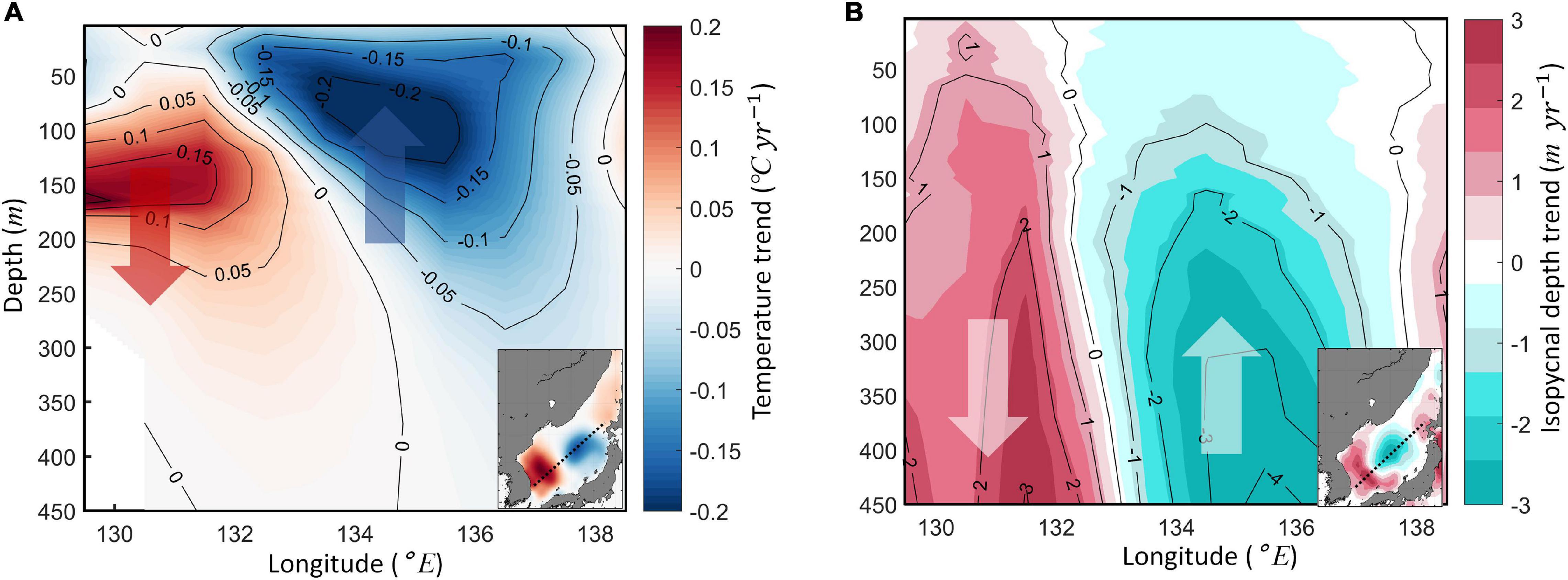
Figure 3. Sectional structures across Regions A and B (shown in black dotted lines in small figures in the lower right corners) of trend differences between the SW and SWS periods (SWS–SW), of (A) subsurface temperature anomaly and (B) isopycnals between SW and SWS periods. The small figures within panels (A,B) are the same as those in Figures 2C,E, indicating the spatial pattern of the trend differences of subsurface temperature and isopycnals, respectively. Each arrow indicates the seawater or volume transport. Arrows pointing upwards mean upwelling and arrows pointing downwards mean downwelling processes, respectively.

The flow characteristics of EKWC is examined by considering the trends in the warm water transport by the ocean currents in the upper 300 m across Regions A and B. The deepening of isopycnals in the southwestern ES (Region A) is shown to be associated with the poleward penetration of EKWC in response to changes in wintertime wind stress curl in the northern ES (Yoon et al., 2016). However, there are no clues on the shoaling isopycnals in Region B. The Region A (129–132°E, 36–39°N) encloses the east coast of Korea, while Region B (134–137°E, 39–42°N) is in the central ES as shown in Figure 1D. Considering the flow pattern of EKWC, it moves northward along the east coast of Korea (through Region A), and meanders eastward at approximately 38°N (Chang et al., 2004), where the current passes through the Region B in the central ES. In view of these, the latitudinal cross-section of ocean currents velocity (as a proxy for the transport) in the upper 300 m across longitudes of Regions A (129–132°E) and B (134–137°E) is examined (Figure 4). Across Region A (Figure 4A), the transport anomaly is more positive extending up to 39°N indicating the poleward penetrating trend of EKWC in consistent with Yoon et al. (2016). However, in Region B, the prominent current flow is eastward and the negative anomalies (Figure 4B) between 39 and 42°N (the latitudes of Region B) mostly indicate the slowing down of eastward movement of EKWC across Region B. This analysis further extended to examine the variability associated with eastward EKWC transport across Mid-ES (133°E, 37–40°N) shown in Figure 5A. Both decadal and interannual signals of transport in Mid-ES were observed to weaken during the SWS period compared to the SW period (Figure 5B). The weakened transport of EKWC can result in large accumulation of warm waters of EKWC in the western ES, which can possibly result in the peak warming trend at deeper levels in Region A compared to the peak cooling trend relatively at higher levels in Region B (Figure 3A). Overall the results indicate the role of northeasterly wind stress anomalies over ES during the SWS period resulting in the heaving effects observed in both Regions A and B with a corresponding change in the flow of EKWC. Therefore, the weakening of the eastward flow of EKWC under the influence of the strengthened northerly wind stress and wind stress curl-induced convergence and divergence may have had a complex effect on the surface warming slowdown and subsurface warming.

FIGURE 4

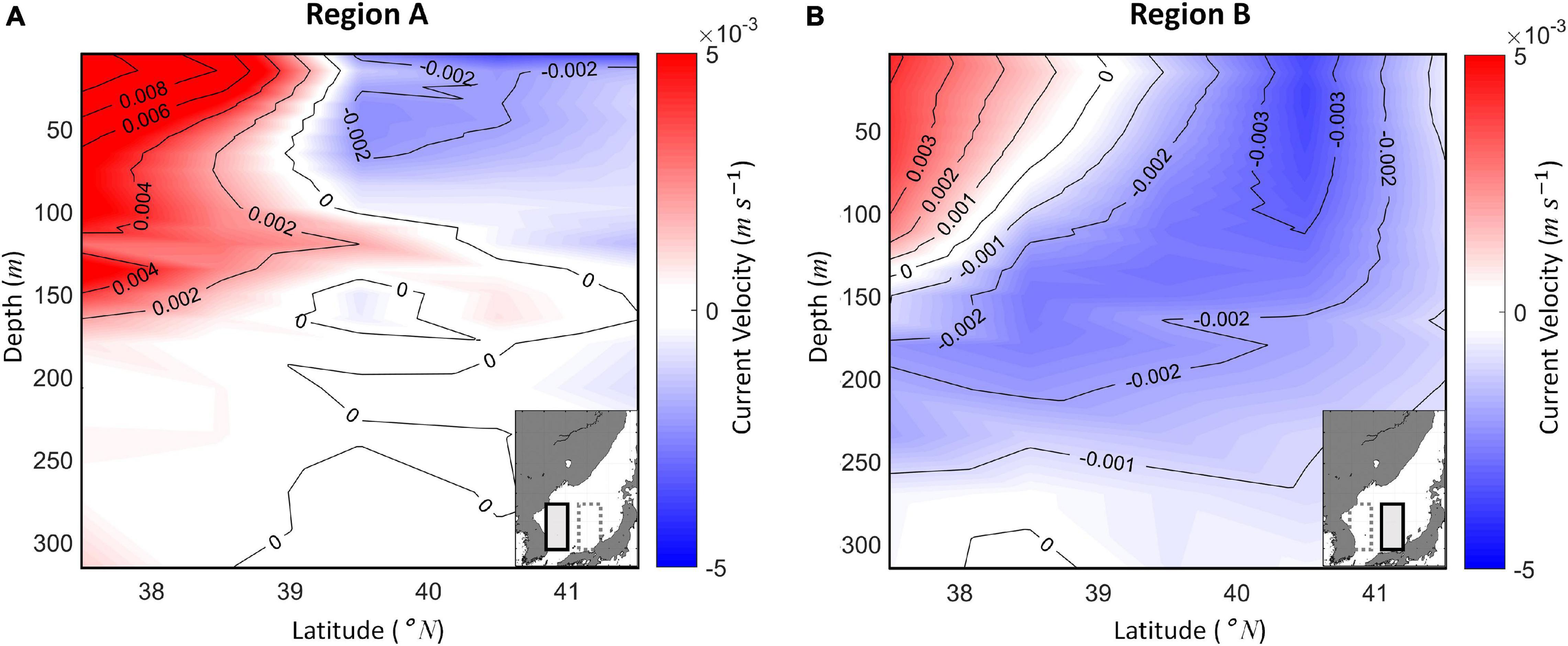
Figure 4. Cross-sectional view of the difference of mean current velocity between the SWS period and the SW period (SWS-SW) in the (A) Region A and (B) Region B. Based on the same latitude, and only the longitude is adjusted to each region. The black boxes in small figures within panels (A,B) indicates the targeted area for each cross-section (gray dotted boxes indicate the opposite region). The region with blue shading indicates the transport has been weakened, and the red shading is vice versa.

FIGURE 5

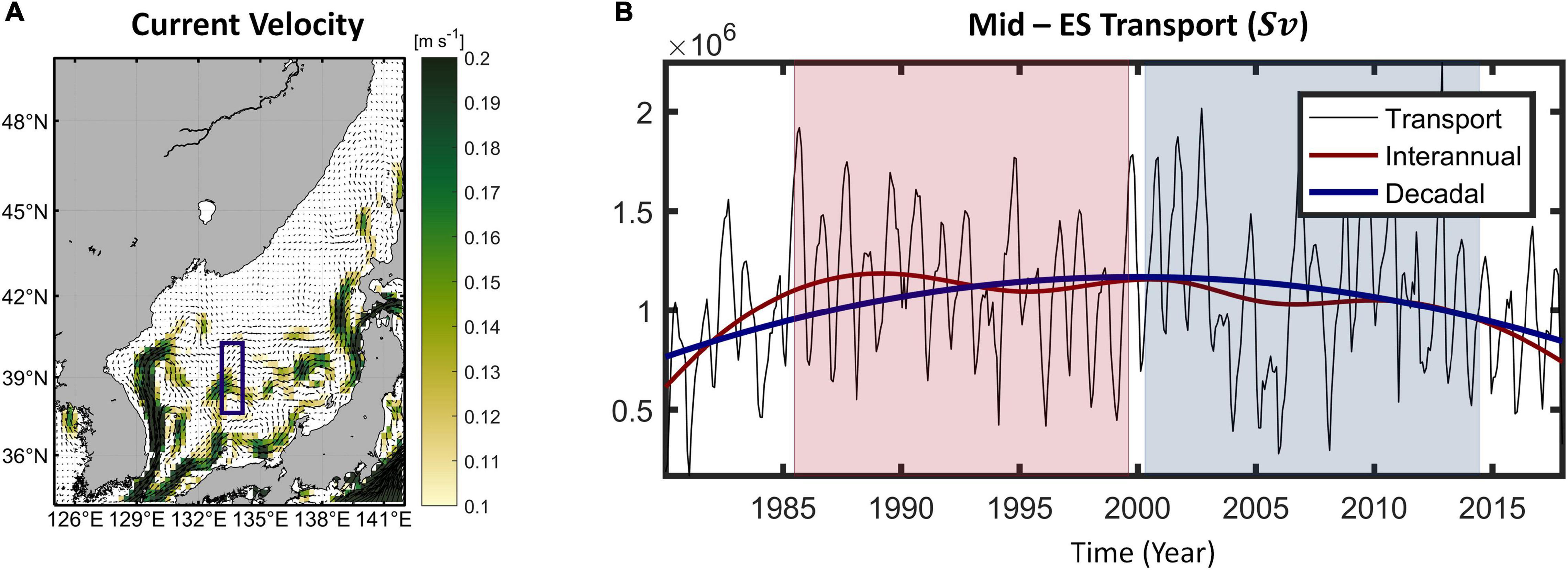
Figure 5. (A) Average spatial pattern of current in the ES in 2017. Shading indicates the current velocity, and only the region with a value higher than 0.1 ms⁻¹ is denoted. The blue rectangle is the region that we set as the Mid-ES (133° E, 37–40° N). (B) Timeseries of the current transport in the Mid-ES. Black, red and blue lines indicate monthly transport, interannual, decadal variation of transport in the Mid-ES, respectively.

In order to analyze the timing of temperature change according to the change in wind and transport, the decadal variation of the three variables (Wind stress curl, Transport of Mid-ES, Subsurface temperature anomaly between 100 and 300 m depth) was examined. As air-sea interactions occur across all spatial and timescales (Wu et al., 2019), here our focus is on the interannual or decadal component of variations in air-sea interactions. In Region A, the decadal wind stress curl variation turned from a positive phase to a negative phase in the late 1990s (Figure 6A). After the early 2000s, the trends of transport and subsurface temperature anomalies changed accordingly. As transport decreases, the trend of subsurface temperature anomalies shifted to positive phases in Region A, which means that warm water that could not flow eastward could accumulate in Region A, causing an increase in temperature at the subsurface. However, in Region B, the decadal wind stress curl variation turned from a negative to a positive phase in the late 1990s, accompanied by negative trends in the transport and subsurface temperature anomaly after the early 2000s (Figure 6B). These patterns also well-matched with the spatial trend change during the SWS period compared to the SW period (Figures 2B,C, 4A,B). Likewise, the rapid decrease in subsurface temperature anomalies with decreased transport and following shoaled isopycnals in Region B since 2000 is explained by the strengthened northerly wind stress and positive wind stress curl inducing horizontal divergence and vertical upwelling. Furthermore, it is interesting to note that there is a significant (∼3 years) time lag between the timing of changes in trends of wind stress curl and other variables. The result of the lead-lag correlation between the wind stress curl and isopycnals in Regions A and B also represent that there are about 30–40 months lag between the wind forcing and oceanic responses (not shown). This lag is seemingly the time it takes for the wind force to affect the basin-scale circulation, which is consistent with the result of Philander (1999), who stated that the time lag of the wind force modulates the ocean circulation.

FIGURE 6

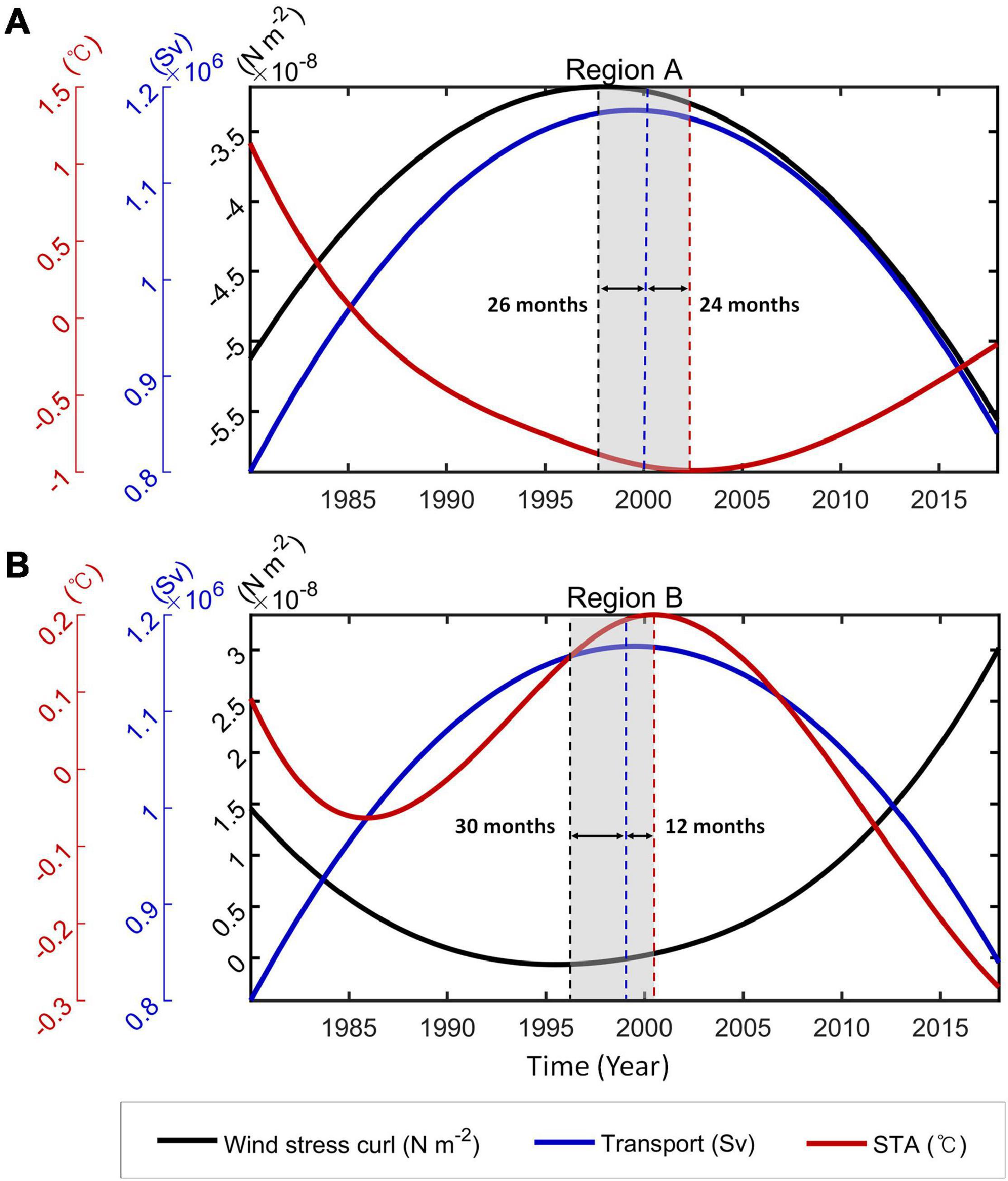
Figure 6. Time series of the decadal IMF of each variable in (A) Region A and (B) Region B. Black, blue, red lines indicate the wind stress curl, volume transport at Mid-ES, and subsurface temperature anomaly (STA), respectively. Each dotted line indicates the conversion point and gray shaded parts imply the time lag (∼3 years) between them.

Spatial and Temporal Variations of Ocean Heat Content Modulated by Sea Surface Wind

Temperature changes due to wind and transport variation ultimately cause coherent changes in OHC as well. During the SWS period, strong increase (approximately 0.5×10⁸Jm²yr⁻¹) and decrease (approximately −1×10⁸Jm²yr⁻¹) in the OHC were found in Regions A and B, respectively (Figure 7A). The ${\mathbf{\text{H}}}_{\mathit{Nonsteric}}^{{}^{\prime }}$ appears to be well following the positive and negative trends of the overall OHC (${\mathbf{\text{H}}}_{\mathit{SLA}}^{{}^{\prime }}$) in Regions A and B during the SWS period (yellow shaded in Figures 7B,C), but the trend and the temporal variation of ${\mathbf{\text{H}}}_{\mathit{Steric}}^{{}^{\prime }}$ was relatively weak compared to ${\mathbf{\text{H}}}_{\mathit{SLA}}^{{}^{\prime }}$ and ${\mathbf{\text{H}}}_{\mathit{Nonsteric}}^{{}^{\prime }}$ (blue vs. black and red in Figures 7B,C). This is consistent with a previous study demonstrating that the heaving effect is more pronounced than the steric effect on decadal and interannual OHC variations in the ES (Yoon et al., 2016). The sea-level change due to the wind stress curl is more consistent with the OHC change than the steric effect during the SWS period. Moreover, because the heaving effect may be affected by the current, the transport volume of the Tsushima Warm Current (TWC) meandering from the southwest of the ES was also investigated (not shown). The analysis was performed to investigate the influence of the TWC on SWS using ORAS4 data, but the volume transport through the Korea Strait was almost constant, suggesting that there is no additional intrusion that can cause the heaving effect. An increase in the OHC in Region A (Figure 7B) and a rapid decrease in the OHC in Region B (Figure 7C) due to the wind effect was confirmed. The total OHC change due to subsurface warming with downwelling in Region A was estimated to be approximately 2×10⁹Jm², and that of the surface cooling with upwelling in Region B to approximately −1×10⁹Jm² during the entire SWS period. Although this study focused on the SWS for 15 years, before 2000 and after 2015, there are some different subsurface warming processes. In particular, after 2015, the dipole pattern reported in this study was not maintained; rather, the sea surface and subsurface in both Regions A and B gained heat. Thus, this study effectively demonstrated such periodic decadal events in the ES.

FIGURE 7

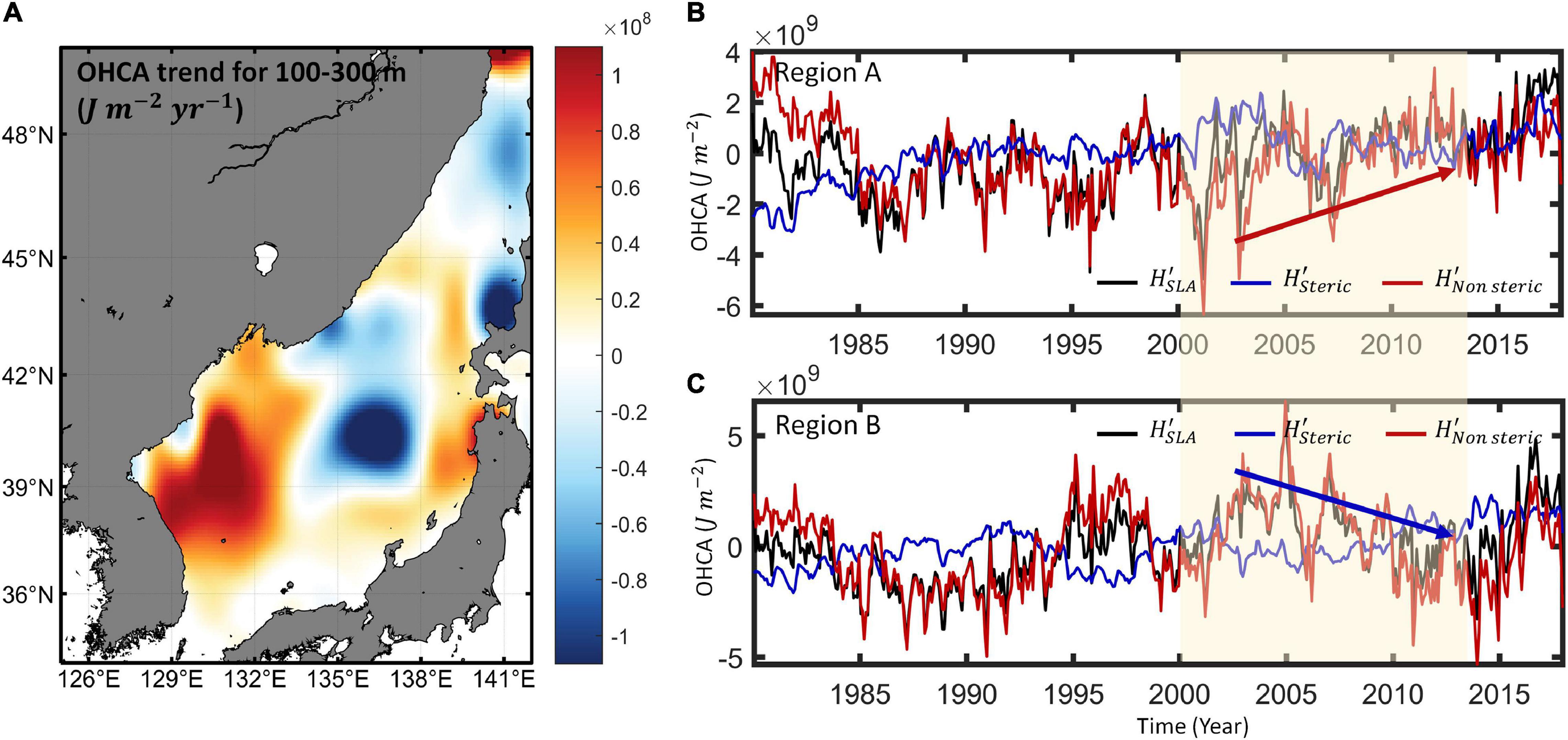
Figure 7. (A) Spatial pattern of the ocean heat content (OHC) trend in the intermediate layer (100–300 m) during the SWS period. Time series of the OHC anomaly (OHCA) in (B) Region A and (C) Region B. Yellow rectangular shading in panels (B,C) represents the SWS periods. Red and blue arrows indicate the increasing and decreasing OHC trends, respectively. Black, blue, and red lines indicate ${\mathbf{\text{H}}}_{\mathit{SLA}}^{{}^{\prime }}$, ${\mathbf{\text{H}}}_{\mathit{Steric}}^{{}^{\prime }}$, and ${\mathbf{\text{H}}}_{\mathit{Nonsteric}}^{{}^{\prime }}$, respectively.

In summary, wind stress-driven weakened ocean current transport to the eastern ES and the wind stress curl-driven horizontal convergence and divergence with the dipole pattern, ultimately leading to the SWS in the ES. The horizontal convergence and divergence in Regions A and B induce downwelling and upwelling, which warms (cools) subsurface (surface) water, as schematized in Figure 8. The primary forcing mechanism is the strengthened northerly wind over the central ES, inducing anticyclonic and cyclonic wind stress curl in the western and eastern ES (Regions A and B), respectively, during the SWS period. The strengthened northerly wind forcing since 2000 is linked to changes in the East Asian Winter Monsoon (EAWM), as quantitatively represented by the sea level pressure (SLP) difference between the SH and East Asian regions, defined as the EAWM index (EAWMI). The EAWMI used by Ding et al. (2014) gradually increased and became positive in the 2000s, indicative of a strengthened EAWM during the 2000s compared to the 1990s (Figure 9A). Thus, the SWS is found in the ES with the strengthening of the EAWM and northerly wind over the central ES during the SWS period (Figure 9B). Spatial patterns of SLP trends before and after 2000 show a rapid change in the SH and East Asia regions during the SWS period, as reflected in the EAWMI (Figures 9C,D). The EAWM has been strengthening since the 2000s, leading to the stronger northerly wind in the central ES, downwelling and upwelling in the western and eastern ES, and SWS in the ES.

FIGURE 8

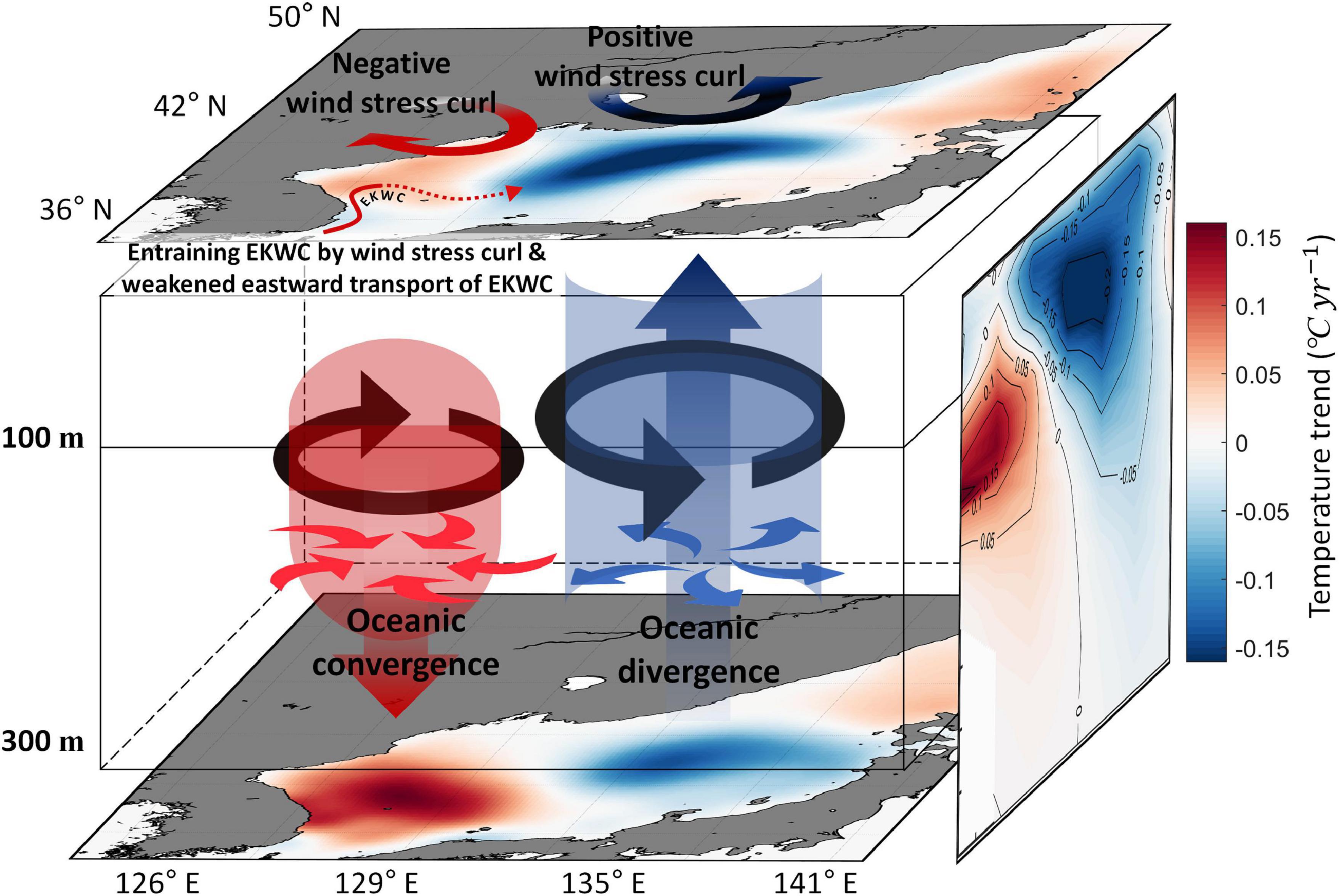
Figure 8. Conceptual schematics representing the wind stress curl-driven convergence (downwelling) and divergence (upwelling) processes in the Regions A and B during the SWS period in the western and eastern ES, respectively. The red line and the red dotted arrow indicate bifurcating poleward entrained EKWC and weakened eastward transport of EKWC, respectively, due to strengthened negative wind stress curl during the SWS period.

FIGURE 9

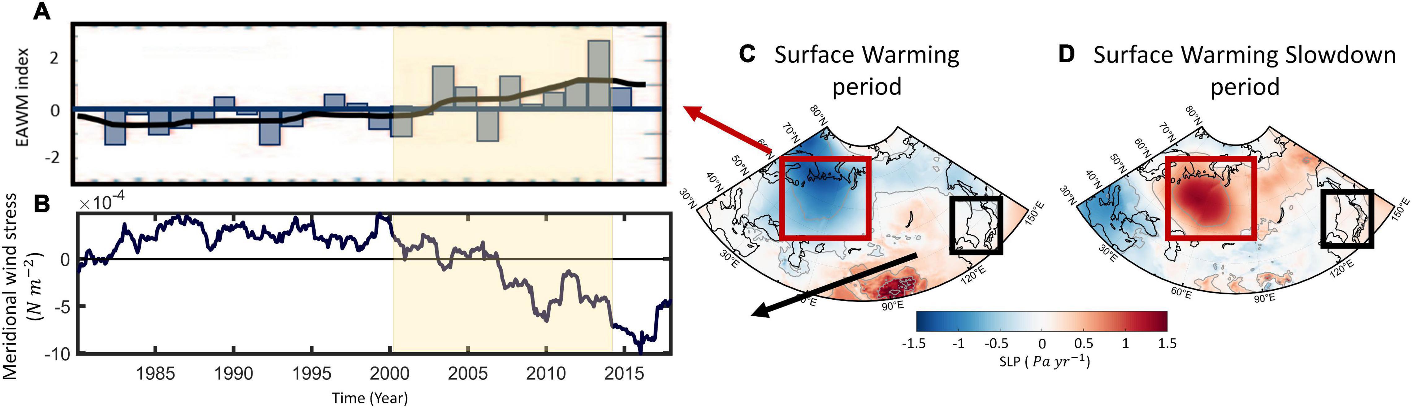
Figure 9. (A) East Asian Winter Monsoon Index (EAWM) (cited from Ding et al., 2014). (B) Meridional wind stress in the ES from 1979 to 2017 and sea level pressure trend of the Northern Hemisphere during (C) 1985–1999 (left), (D) 2000–2014 (right), respectively. Red boxes indicate the Siberian High region. Black boxes indicate the ES.

Conclusion

We conducted a trend analysis of sea surface and subsurface temperature anomalies, SLA, isopycnals, and wind stress curl, and our findings are summarized as follows:

1. From 2000 to 2014, a significant surface warming slowdown occurred in the ES compared to the previous warming period (1985–1999), which was defined as the SWS period. During this period, while the water temperature in the upper 100 m showed a negative trend, the subsurface temperature or temperature at the intermediate layer (between 100 and 300 m) showed a positive trend.

2. The spatial pattern of the long-term trend during the SWS period of subsurface temperature at the intermediate layer was similar to those of the SLA, isopycnals, and wind stress curl. There was a higher (lower) sea level and deepened (shoaled) isopycnals in the western (eastern) ES or Region A (Region B) during the SWS period. This dipole pattern is consistent with the horizontal convergence (downwelling) and divergence (upwelling) patterns in the western and eastern ES, respectively.

3. During the SWS period, anticyclonic and cyclonic circulations in Regions A and B, respectively, are associated with negative and positive wind stress curls induced by the northerly winds in the central ES. Furthermore, strengthened northerly wind stress also weakened eastward EKWC resulting in the large accumulation of warm water from EKWC in western ES. Consequently, the convergence in Region A drives downwelling of relatively warm water from the surface to the intermediate layer, whereas the divergence in Region B causes upwelling of cold subsurface water to the upper 100 m at a lag of approximately 3 years. Owing to the dipole patterns of convergence and divergence in each region, the surface warming trend in the ES could be slowed down.

Therefore, these results suggest the influence of large-scale teleconnections liked to the SH and EAWM on the warming trend of marginal seas such as the ES by modulating the local air-sea interactions.

Data Availability Statement

The raw data supporting the conclusions of this article will be made available by the authors, without undue reservation.

Author Contributions

YJ and Y-HJ contributed to the conceptualization and formal analysis of the study. YJ collected the data. Y-HJ, SN, J-IK, and UU contributed to the methodology and investigation. YJ initially wrote this manuscript. SN, J-IK, UU, and Y-HJ revised and edited the manuscript. YJ and UU contributed to the visualization. Y-HJ supervised this article. All authors have read and agreed to the published version of the manuscript.

Funding

This study was supported by the National Research Foundation of Korea (NRF) grant funded by the Korea Government (MSIP) (NRF-2018R1A2B2006555). SN was partially supported by the project titled “Deep Water Circulation and Material Cycling in the East Sea (20160040)”, funded by the Ministry of Oceans and Fisheries, South Korea.

Conflict of Interest

The authors declare that the research was conducted in the absence of any commercial or financial relationships that could be construed as a potential conflict of interest.

Publisher’s Note

All claims expressed in this article are solely those of the authors and do not necessarily represent those of their affiliated organizations, or those of the publisher, the editors and the reviewers. Any product that may be evaluated in this article, or claim that may be made by its manufacturer, is not guaranteed or endorsed by the publisher.

Footnotes

1. ^ coriolis.eu.org

References

Balmaseda, M. A., Trenberth, K. E., and Källén, E. (2013). Distinctive climate signals in reanalysis of global ocean heat content. Geophys. Res. Lett. 40, 1754–1759. doi: 10.1002/grl.50382

CrossRef Full Text | Google Scholar

Belkin, I. M. (2009). Rapid warming of large marine ecosystems. Prog. Oceanogr. 81, 207–213. doi: 10.1016/j.pocean.2009.04.011

CrossRef Full Text | Google Scholar

Chambers, D. P., Tapley, B. D., and Stewart, R. H. (1997). Long-period ocean heat storage rates and basin-scale heat fluxes from TOPEX. J. Geophys. Res. Oceans 102, 10525–10533. doi: 10.1029/96jc03644

CrossRef Full Text | Google Scholar

Chang, K. I., Teague, W. J., Lyu, S. J., Perkins, H. T., Lee, D. K., Watts, D. R., et al. (2004). Circulation and currents in the southwestern East/Japan Sea: overview and review. Prog. Oceanogr. 61, 105–156. doi: 10.1016/j.pocean.2004.06.005

CrossRef Full Text | Google Scholar

Chen, X., and Tung, K.-K. (2014). Varying planetary heat sink led to global-warming slowdown and acceleration. Science 345, 897–903. doi: 10.1126/science.1254937

PubMed Abstract | CrossRef Full Text | Google Scholar

Ding, Y., Liu, Y., Liang, S., Ma, X., Zhang, Y., Si, D., et al. (2014). Interdecadal variability of the East Asian winter monsoon and its possible links to global climate change. J. Meteorol. Res. 28, 693–713. doi: 10.1007/s13351-014-4046-y

CrossRef Full Text | Google Scholar

England, M., McGregor, S., Spence, P., Meehl, G. A., Timmermann, A., Cai, W., et al. (2014). Recent intensification of wind-driven circulation in the Pacific and the ongoing warming hiatus. Nat. Clim. Change 4, 222–227. doi: 10.1038/nclimate2106

CrossRef Full Text | Google Scholar

Gallagher, S. J., Sagawa, T., Henderson, A. C. G., Saavedra-Pellitero, M., De Vleeschouwer, D., Black, H., et al. (2018). East Asian monsoon history and paleoceanography of the Japan Sea over the last 460,000 years. Paleoceanogr. Paleoclimatol. 33, 683–702. doi: 10.1029/2018pa003331

CrossRef Full Text | Google Scholar

Gamo, T. (1999). Global warming may have slowed down the deep conveyor belt of a marginal sea of the northwestern Pacific: Japan Sea. Geophys. Res. Lett. 26, 3137–3140. doi: 10.1029/1999GL002341

CrossRef Full Text | Google Scholar

Gamo, T. (2011). Dissolved oxygen in the bottom water of the Sea of Japan as a sensitive alarm for global climate change. Trends Anal. Chem. 30, 1308–1319. doi: 10.1016/j.trac.2011.06.005

CrossRef Full Text | Google Scholar

Gill, A. E., and Niller, P. P. (1973). The theory of the seasonal variability in the ocean. Deep Sea Res. Oceanogr. Abst. 20, 141–177. doi: 10.1016/0011-7471(73)90049-1

CrossRef Full Text | Google Scholar

Gordon, A. L., and Giulivi, C. F. (2004). Pacific decadal oscillation and sea level in the Japan/East sea. Deep Sea Res.Part I Oceanogr. Res. Pap. 51, 653–663. doi: 10.1016/j.dsr.2004.02.005

CrossRef Full Text | Google Scholar

Han, L., and Yan, X.-H. (2018). Warming in the Agulhas region during the global surface warming acceleration and slowdown. Sci. Rep. 8:13452. doi: 10.1038/s41598-018-31755-1

PubMed Abstract | CrossRef Full Text | Google Scholar

Han, M., Cho, Y.-K., Kang, H.-W., and Nam, S. (2020). Decadal changes in meridional overturning circulation in the East Sea (Sea of Japan). J. Phys. Oceanogr. 50:6. doi: 10.1175/jpo-d-19-0248.1

CrossRef Full Text | Google Scholar

IPCC (2013). “Climate change 2013: the physical science basis,” in Contribution of Working Group I to the Fifth Assessment Report of the Intergovernmental Panel on Climate Change, eds T. F. Stocker et al. (Cambridge: Cambridge University Press), 1585.

Google Scholar

IPCC (2014). “Climate change 2014: synthesis report,” in Contribution of Working Groups I, II and III to the Fifth Assessment Report of the Intergovernmental Panel on Climate Change, eds R. K. Core Writing Team Pachauri and L. A. Meyer (Geneva: IPCC), 151.

Google Scholar

Jeong, J. I., and Park, R. J. (2017). Winter monsoon variability and its impact on aerosol concentrations in East Asia. Environ. Pollut. 221, 285–292. doi: 10.1016/j.envpol.2016.11.075

PubMed Abstract | CrossRef Full Text | Google Scholar

Kim, K., Kim, K.-R., Min, D.-H., Volkov, Y., Yoon, J.-H., and Takematsu, M. (2001). Warming and structural changes in the East (Japan) Sea: a clue to future changes in global oceans? Geophys. Res. Lett. 28, 3293–3296. doi: 10.1029/2001gl013078

CrossRef Full Text | Google Scholar

Kosaka, Y., and Xie, S.-P. (2016). The tropical Pacific as a key pacemaker of the variable rates of global warming. Nat. Geosci. 9, 669–673. doi: 10.1038/ngeo2770

CrossRef Full Text | Google Scholar

Lee, D. K. (1998). Ocean surface winds over the seas around Korea measured by the NSCAT (NASA Scatterometer). J. Korean Soc. Remote Sens. 14, 37–52.

Google Scholar

Lee, E.-Y., and Park, K.-A. (2019). Change in the recent warming trend of sea surface temperature in the East Sea (Sea of Japan) over decades (1982–2018). Remote Sens. 11:2613. doi: 10.3390/rs11222613

CrossRef Full Text | Google Scholar

Lee, J.-Y., Kang, D.-J., Kim, I.-N., Rho, T., Lee, T., Kang, C.-K., et al. (2009). Spatial and temporal variability in the pelagic ecosystem of the East Sea (Sea of Japan): a review. J. Mar. Syst. 78, 288–300. doi: 10.1016/j.jmarsys.2009.02.013

CrossRef Full Text | Google Scholar

Lee, S.-K., Park, W., Baringer, M. O., Gordon, A. L., Huber, B., and Liu, Y. (2015). Pacific origin of the abrupt increase in Indian Ocean heat content during the warming hiatus. Nat. Geosci. 8, 445–449. doi: 10.1038/ngeo2438

CrossRef Full Text | Google Scholar

Levitus, S., Antonov, J. I., Boyer, T. P., Baranova, O. K., Garcia, H. E., Locarnini, R. A., et al. (2012). World ocean heat content and thermosteric sea level change (0-2000 m), 1955-2010. Geophys. Res. Lett. 39, 1–5. doi: 10.1029/2012gl051106

CrossRef Full Text | Google Scholar

Liao, E., Lu, W., Yan, X.-H., Jiang, Y., and Kidwell, A. (2015). The coastal ocean response to the global warming acceleration and hiatus. Sci. Rep. 5:16630. doi: 10.1038/srep16630

PubMed Abstract | CrossRef Full Text | Google Scholar

Lyman, J. M., Good, S. A., Gouretski, V. V., Ishii, M., Johnson, G. C., Palmer, M. D., et al. (2010). Robust warming of the global upper ocean. Nature 465, 334–337. doi: 10.1038/nature09043

PubMed Abstract | CrossRef Full Text | Google Scholar

Nam, S., Yoon, S.-T., Park, J.-H., Kim, Y. H., and Chang, K.-I. (2016). Distinct characteristics of the intermediate water observed off the east coast of Korea during two contrasting years. J. Geophys. Res. Oceans 121, 5050–5068. doi: 10.1002/2015jc011593

CrossRef Full Text | Google Scholar

Philander, S. G. (1999). A review of tropical ocean-atmosphere interactions. Tellus B 51, 71–90. doi: 10.1034/j.1600-0889.1999.00007

PubMed Abstract | CrossRef Full Text | Google Scholar

Purkey, S. G., and Johnson, G. C. (2010). Warming of global abyssal and deep Southern Ocean waters between the 1990s and 2000s: contributions to global heat and sea level rise budgets. J. Clim. 23, 6336–6351. doi: 10.1175/2010jcli3682.1

CrossRef Full Text | Google Scholar

Schroeder, K., Chiggiato, J., Josey, S. A., Borghini, M., Aracri, S., and Sparnocchia, S. (2017). Rapid response to climate change in a marginal sea. Sci. Rep. 7:4065. doi: 10.1038/s41598-017-04455-5

PubMed Abstract | CrossRef Full Text | Google Scholar

Talley, L. D., Min, D.-H., Lobanov, V. B., Luchin, V. A., Ponomarev, V. I., Salyuk, A. N., et al. (2006). Japan/East Sea water masses and their relation to the sea’s circulation. Oceanography 19, 32–49. doi: 10.5670/oceanog.2006.42

CrossRef Full Text | Google Scholar

Wang, L., and Koblinsky, C. (1997). Can the TOPEX/Poseidon altimetry data be used to estimate air-sea heat flux in the North Atlantic? Geophys. Res. Lett. 24, 139–142. doi: 10.1029/96gl03695

CrossRef Full Text | Google Scholar

Wu, X., Xu, Q., Li, G., Liou, Y.-A., Wang, B., Mei, H., et al. (2019). Remotely-observed early spring warming in the southwestern yellow sea due to weakened winter monsoon. Remote Sens. 11:2478. doi: 10.3390/rs11212478

CrossRef Full Text | Google Scholar

Wu, Z., and Huang, N. E. (2009). Ensemble empirical mode decomposition: a noise-assisted data analysis method. Adv. Adapt. Data Anal. 01, 1–41. doi: 10.1142/s1793536909000047

CrossRef Full Text | Google Scholar

Yan, X.-H., Boyer, T., Trenberth, K., Karl, T. R., Xie, S.-P., Nieves, V., et al. (2016). The global warming hiatus: slowdown or redistribution? Earths Future 4, 472–482. doi: 10.1002/2016EF000417

PubMed Abstract | CrossRef Full Text | Google Scholar

Yoon, J.-H., Abe, K., Ogata, T., and Wakamatsu, Y. (2005). The effects of wind-stress curl on the Japan/East Sea circulation. Deep Sea Res. Part II Top. Stud. Oceanogr. 52, 1827–1844. doi: 10.1016/j.dsr2.2004.03.004

CrossRef Full Text | Google Scholar

Yoon, S.-T., Chang, K.-I., Na, H., and Minobe, S. (2016). An east-west contrast of upper ocean heat content variation south of the subpolar front in the East/Japan Sea. J. Geophys. Res. Oceans 121, 6418–6443. doi: 10.1002/2016jc011891

CrossRef Full Text | Google Scholar

Yoon, S.-T., Chang, K.-I., Nam, S., Rho, T., Kang, D.-J., Lee, T., et al. (2018). Re-initiation of bottom water formation in the East Sea (Japan Sea) in a warming world. Sci. Rep. 8:1576. doi: 10.1038/s41598-018-19952-4

PubMed Abstract | CrossRef Full Text | Google Scholar