Mixed layer eddies supply nutrients to enhance the spring phytoplankton bloom

Mixed layer eddies resulting from baroclinic instability of fronts convert horizontal buoyancy gradients into vertical stratification, shoaling the mixed layer. In light-limited regimes – high-latitudes – this process can initiate phytoplankton blooms prior to the springtime warming. The question is whether mixed layer eddies can enhance the spring bloom by delivering nutrients from beneath the mixed layer. We couple a submesoscale-resolving model (SUB) with a simple ecosystem model and examine the role of mixed layer eddies on the development of the spring bloom. We compare the SUB simulation to two coarser resolution (10 km) simulations, one that includes a mixed layer eddy parameterization (MLE) and another that prescribes the restratification from SUB and advects the biogeochemical tracers using geostrophic velocities (NVF). The MLE simulates restratification of the mixed layer and bloom onset, but the spring bloom has a deficit of 10–13% in the new production compared to SUB. The NVF has the same restratification as SUB, and with no vertical flux of nutrients, leads to a spring bloom with a 32–40% new production deficit compared to SUB. Submesoscale processes lead to exchange across the mixed layer base, which is not represented in coarse resolution model simulations, even with mixed layer eddy parameterizations. Our results show that nutrients supplied by mixed layer eddies are important to enhance the spring bloom.

1 Introduction

Horizontal gradients of buoyancy in the surface mixed layer of the ocean give rise to submesoscale instabilities that are characterized by O (1) Rossby and Richardson numbers and length scales of 0.1–10 km. Surface-intensified currents support frontogenesis and induce vertical motion (Thomas et al., 2008; Mahadevan et al., 2010; McWilliams, 2016), while mixed layer eddies tend to slump isopycnals and increase density stratification, thereby changing the depth of the mixed layer (Fox-Kemper et al., 2008; Thomas et al., 2013). However, climate models do not resolve submesoscale ocean dynamics and generally rely on one-dimensional processes to alter the oceanic mixed layer depth. The absence of three-dimensional, eddy-driven restratifying processes is one of the reasons the mixed layer is deeper in global models than in the observational data (Oschlies, 2002; Fox-Kemper et al., 2008; Thomas et al., 2008). This issue is addressed by an effective parameterization developed for mixed layer eddies (Fox-Kemper et al., 2008; Fox-Kemper and Ferrari, 2008), which contributes to shallower mixed layer depths, particularly in high-latitude regions.

The shallowing of the mixed layer is crucial for phytoplankton growth in light limited regimes, such as the subpolar North Atlantic at the end of the winter (e.g. Sverdrup, 1953; Martinez et al., 2011; Diaz et al., 2021). The North Atlantic is one of the world’s most intense oceanic sinks of atmospheric CO2 per unit area (Takahashi et al., 2009) and is particularly sensitive to restratifying processes, as seasonal phytoplankton blooms (Bagniewski et al., 2011) are triggered by the shoaling of the mixed layer.

Classical theory posits that spring blooms occur in light-limited regimes when the shoaling mixed layer reaches a critical depth, where the growth of trapped phytoplankton in nutrient-rich winter waters exceeds their mortality (Sverdrup, 1953). Traditionally, it was thought that the mixed layer shoals due to springtime solar heating. But, observations show a late-winter to early-spring onset of the bloom, which is explained by several theories that include plankton dilution relieving grazing pressure (Behrenfeld, 2010; Behrenfeld and Boss, 2014), decreased turbulent mixing (Taylor and Ferrari, 2011), and eddy-driven stratification (Mahadevan et al., 2012). Of these processes, eddy-driven restratification can significantly alter the mixed layer depth over vast regions. In the wintertime, ocean fronts promote submesoscale baroclinic instability in the mixed layer, which results in mixed layer eddies (Karimpour et al., 2018). While buoyancy loss and downfront winds deepen the mixed layer, mixed layer eddies tend to slump isopycnals (Mahadevan et al., 2010) and achieve restratification when the surface forcing weakens, sometimes even in the late winter or early spring. In these regions, it is not just the solar heat flux, but also eddy-driven restratification that controls the intensity and timing of springtime phytoplankton blooms (Mahadevan et al., 2012).

In contrast to surface heating, the stratification resulting from mixed layer eddy dynamics is patchy, and its horizontal heterogeneity provides alternative pathways for fluxing nutrients and carbon, thereby enhancing the vertical exchange between mixed layer and pycnocline (Omand et al., 2015; Lévy et al., 2018; Freilich and Mahadevan, 2019). In particular, since advection occurs along density surfaces, tilting isopycnals facilitate the vertical transport of nutrients to the mixed layer, which can significantly affect the primary production in nutrient-limited regimes (Pasquero et al., 2005; Freilich and Mahadevan, 2019). While mixed layer eddy parameterizations are effective in improving the mixed layer depth in climate models (Fox-Kemper and Ferrari, 2008), it is unclear if they are able to capture the vertical flux of biogeochemical tracers, particularly across the base of the mixed layer.

This study addresses the contribution of the eddy-driven flux of nutrients to the spring bloom in a high-latitude environment. In addition, we assess whether existing mixed layer eddy parameterizations (Fox-Kemper et al., 2008; Omand et al., 2015) capture such a process. In section 2, we explain the numerical set up for the submesoscale-resolving simulation and describe its evolution in section 3. In section 4, we employ two coarse-resolution simulations. We used Fox-Kemper et al. (2008) parameterization in one of the coarse-resolution simulations and prescribe the resolved restratification while imposing zero vertical flux in another. The coarse-resolution simulations are then compared with the high-resolution simulation in terms of restratification and shoaling of the mixed layer. In section 5, we describe how each simulation reproduces the springtime phytoplankton bloom, and we compare them in terms of the vertical flux of nutrients and production in section 6. In section 7, we discuss the main results and present the conclusions.

2 Model setup

We use a three-dimensional process model (Oceananigans.jl, Ramadhan et al., 2020) to explore upper ocean submesoscale dynamics and estimate the nutrient flux across the base of the mixed layer. This model solves the fully non-hydrostatic Boussinesq equations based on the architecture of the Massachusetts Institute of Technology general circulation model (MITgcm, Marshall et al., 1997). We used adaptive time step based on the CFL condition and a fifth-order WENO (weighted essentially non-oscillatory) advection scheme for all simulations.

The model domain consists of a periodic zonal channel on the f-plane, centered at 60°N. We impose solid walls at the northern and southern boundaries, and free-slip boundary conditions at the lateral walls and bottom. The domain has 100 km in the west-east, x-direction, and 500 km in the south-north, y-direction, and it is 1000 m deep (H), with 50km-wide sponge layers along the northern and southern boundaries to prevent the reflection of waves. Depending on the experiment, the horizontal grid resolution is chosen to be 1 km or 10 km throughout the domain (explained later in sections 4 and 5). The vertical z-direction is discretized with 48 grid cells that are non-uniform in size, ranging from 1 m near the surface and increasing to 47 m at depth. The z nodes at the face of the cells are defined by

$\begin{array}{ll}z\left(n\right)=\left[H\cos \left(\frac{n\pi }{96}\right)-H\right]\text{\hspace{0.17em}for\hspace{0.17em}}n\in \left\{0,1,\dots ,49\right\}& (1)\end{array}$

The model is initialized with typical midwinter conditions. The background density is derived from Argo float profiles (Argo, 2020) of February in the North Atlantic (Figure 1A)

FIGURE 1

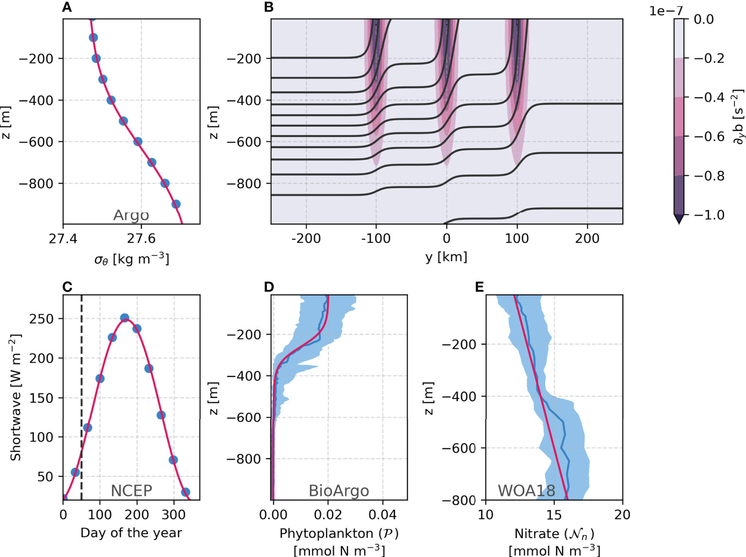
Figure 1 Initial background profile for density (A), initial buoyancy and lateral gradient of buoyancy (B), the surface photosynthetically active radiation (ℒ₀, C), the phytoplakton concentration (D), and nitrate concentration (E). Data is shown in blue and the modeled functions in red. Shaded areas represent the 20^th-80^th percentiles.

$\begin{array}{ll}\overline{\rho }\left(z\right)=-0.147\tanh \left[2.6\frac{\left(z+623\right)}{1000}\right]-1027.6& (2)\end{array}$

Following Karimpour et al. (2018), the vertical density structure is overlaid with three intense density fronts 100 km apart, with a horizontal buoyancy gradient ∇_hb = 10^-7 s^-2 at the surface and decaying to the average pycnocline (Figure 1B), defined by

$\begin{array}{ll}\begin{array}{ll}b\left(x,y,z\right){|}_{t=0}=-\frac{g\overline{\rho }}{{\rho }_0}\hfill & \{0.4\left[\tanh \left(\frac{z+500}{300}\right)+1\right]\hfill \\ {\displaystyle \sum _i}\tanh \left[\frac{y-w_a\left(c_i+\sin \frac{2\pi x}{w_{\lambda }}\right)}{0.5L}\right]\},\hfill \end{array}& (3)\end{array}$

where g= 9.82 m s^-2 is the gravity acceleration, ρ₀ = 1026 kg m^-3 is the reference density, c_i = [-100, 0, 100] km is the x-position of each front, and L = 25 km the front width. We add wiggles of amplitude w_a = 1 km and wavelength w_λ = 10 km to the initial front paths to trigger baroclinic instability. Lastly, the initial velocity field is in thermal wind balance assuming a level of no motion at the bottom.

The simulations are unforced (i.e. no surface heat flux or winds) to isolate the effects of mixed layer eddies and fronts in transporting nutrients. The turbulent diffusivity coefficient (ĸ) is set to be constant at background values of 10^-5 m² s^-1 since wind forcing and complex topography are absent. The horizontal diffusivity of momentum and tracers is also constant and set to 1 m² s^-1 for the 1 km experiment and 10 m² s^-1 for the 10 km experiments.

We couple a simple Nutrient-Phytoplankton ecosystem model (Bagniewski et al., 2011; Gruber et al., 2006; Freilich and Mahadevan, 2019) with the process model to solve the temporal evolution of phytoplankton (P) in a horizontally inhomogeneous eddy environment. The phytoplankton evolution is given by

$\begin{array}{ll}\begin{array}{c}\hfill {\partial }_{t}P+\underset{\text{advection}}{\underbrace{\nabla ·(\overrightarrow{u}P)}}+\underset{\text{sinking}}{\underbrace{{\partial }_z(w_{s}P)}}=\underset{\text{total\hspace{0.17em}production}}{\underbrace{G\left[\frac{N_n}{(N_n+k_n)}\frac{k_r}{(N_r+k_r)}\frac{N_r}{(N_r+k_r)}\right]P}}\hfill \\ \hfill \underset{\text{loss}}{\underbrace{-m{P}^2}}+\underset{\text{mixing}}{\underbrace{\nabla (\kappa \nabla P)}},\hfill \end{array}& (4)\end{array}$

where $\overrightarrow{u}$ is the total velocity, w_s is the constant sinking speed of the phytoplankton (1 m day^-1). k_n = 0.75 mmol Nm^-3 and k_r = 0.5 mmol Nm^-3 are the half saturation constants for nitrate and ammonium uptake, respectively. Although light-averaging within the mixed layer has been previously employed and compared to observations (Mahadevan et al., 2012), other studies approach this issue differently (e.g., Sarmiento et al., 1993). Assuming the mixing time scale is longer than the photosynthesis reaction time, but shorter than the cell-division time, the light-limited growth is averaged over the mixed layer (Fasham et al., 1990) and is then defined as

$\begin{array}{ll}G\left(z\right)=\{\begin{array}{ll}\frac{1}{h}{\displaystyle {\int }_{-h}^0{G}_0\left(\widehat{z}\right)d\widehat{z}}\hfill & \text{\hspace{0.17em}for }z\ge -h\hfill \\ G_0\left(z\right)\hfill & \text{\hspace{0.17em}for }z<-h\hfill \end{array},& \text{(5a)}\end{array}$

$\begin{array}{ll}{G}_0\left(z\right)=\mu \frac{ℒ\alpha }{\sqrt{{\mu }^2+{(ℒ\alpha )}^2}},& \text{(5b)}\end{array}$

where μ is the maximum growth rate (varied from 0.5 - 1.25 day^-1 to test sensitivity to its value), h is the mixed layer depth defined as the depth that the density is at least 0.03 kg m^-3 higher than the surface density (same as used by Fox-Kemper et al., 2011) and α= 0.0538 m² day^-1 is the initial slope of the photosynthesis-irradiance curve. ℒ is the photosynthetically active radiation given by

$\begin{array}{ll}ℒ\left(z\right)=0.43{ℒ}_0{e}^{-z{K}_d-{\displaystyle {\int }_0^z{K}_{C}C\left(\widehat{z}\right)d\widehat{z}}},& (6)\end{array}$

where ℒ₀ is the incident radiation at the surface. We follow a time series for shortwave radiation to mimic the increasing light availability during the transition from winter to spring (50^th to 130^th day of the year, see Figure 1C). The incident radiation is therefore expressed as

$\begin{array}{ll}{ℒ}_0\left(t\right)=116\sin \left[2\pi \frac{\left(t+50\right)}{375.3}-1.3\right]+132.3& (7)\end{array}$

with t expressed in days. The constants of the exponential light attenuation in the water column are K_d = 0.059 m^-1 and K_C = 0.041 m² mg^-1 due to water and chlorophyll concentration (C), respectively.

The nutrients – expressed as nitrate (N_n ) and ammonium (N_r ) – are advected, mixed, and consumed by phytoplankton. The ammonium was added mainly to differentiate the recycled production from the new production. We use the term “new production” to refer to the nitrate uptake (e.g. Lachkar and Gruber, 2011). The phytoplankton loss term has a mortality rate (m) of 0.015 day^-1 and the multiplicative factor k_r/(N_r+k_r) in the uptake term of Equation 9 ensures that the phytoplankton prefer consuming N_r rather than N_n (Gruber et al., 2006). The nutrients are modeled as

$\begin{array}{ll}{\partial }_t{N}_n+\underset{\text{advection}}{\underbrace{\nabla ·\left(\overrightarrow{u}{N}_n\right)}}=\underset{\text{uptake}}{\underbrace{G\frac{N_n}{\left(N_n+k_n\right)}\frac{k_r}{\left(N_r+k_r\right)}P}}+\underset{\text{mixing}}{\underbrace{\nabla \left(\kappa \nabla N_n\right)}},& \text{(8a)}\end{array}$

$\begin{array}{ll}{\partial }_t{N}_r+\underset{\text{advection}}{\underbrace{\nabla ·\left(\overrightarrow{u}{N}_r\right)}}=-\underset{\text{uptake}}{\underbrace{G\frac{N_r}{\left(N_r+k_r\right)}}}P+\underset{loss}{\underbrace{m{P}^2}}+\underset{\text{mixing}}{\underbrace{\nabla \left(\kappa \nabla N_r\right)}}.& \text{(8b)}\end{array}$

The initial phytoplankton concentration (Equation 11, Figure 1D) is based on BioArgo (Argo, 2020) chlorophyll profiles (using 0.06 for chlorophyll to carbon ratio, Álvarez et al., 2018), and the initial nitrate concentration Equation 9 (Figure 1E) is derived from the World Ocean Atlas 2018 (WOA18, Garcia et al., 2018).

$\begin{array}{ll}P\left(z\right){|}_{t=0}=0.2\tanh \left[\frac{0.02\left(z+300\right)+1}{2}\right],& \text{(9a)}\end{array}$

$\begin{array}{ll}{N}_n\left(z\right){|}_{t=0}=12-\frac{z}{200}.& \text{(9b)}\end{array}$

The averages are computed using profiles within the coordinate range of 45–15°W and 55–65°N from February. We do not explicitly represent the grazing by zooplankton. Instead, we consider nutrient limitation and a quadratic loss term which increases the mortality to account for phytoplankton biomass losses due to higher-trophic level predation (Freilich et al., 2021) and to enhance the phytoplankton response to sporadic nutrient uptake (Freilich and Mahadevan, 2019). Lastly, the ammonium is initialized as zero.

3 The submesoscale-resolving experiment

To quantify the effect of submesoscale vertical fluxes on the ecosystem model, we first use the three-dimensional process model described in section 2 with 1km-horizontal resolution to perform a submesoscale-resolving experiment (hereafter SUB).

The fronts are initially 25 km wide and 100 km distant from each other (Figures 2A, 3A). They evolve in time without any surface forcing to form mixed layer eddies that restratify the ocean in a patchy manner by tilting isopycnals which outcrop from 500 m to the surface (Figure 2). While restratifying, the eddies sharpen the density gradients that also become baroclinically unstable, increasing the kinetic energy of this system (Fox-Kemper et al., 2008; Thomas et al., 2008). The strong vertical velocities reaching hundreds of meters depth at sharp density gradients are typical of submesoscale dynamics (Fox-Kemper et al., 2008; Thomas et al., 2008; Thomas et al., 2013; Erickson et al., 2020). The maximum vertical velocities occur close to the mixed layer base (e.g., the section at Y= 100 km in Figure 2B).

FIGURE 2

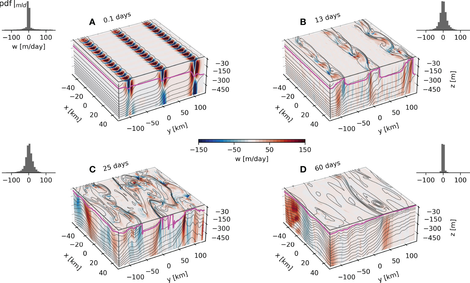
Figure 2 Top 500m density (lines) and vertical velocity (colors) from the 3D experiment output for day 0.1 (A), 13 (B), 25 (C) and 60 (D). The green line represents the mixed layer depth. The 25m average vertical velocity is presented at the surface. The PDFs of the vertical velocity at the mixed layer depth are presented at the top of every panel.

FIGURE 3

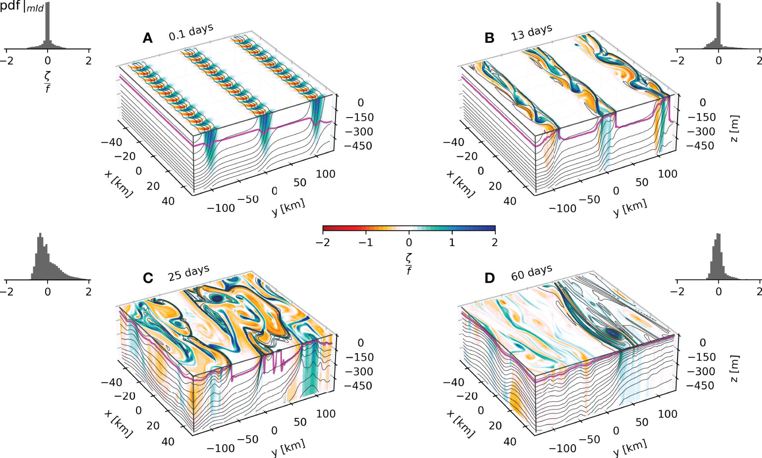
Figure 3 Top 500m Rossby Number contours from the 3D experiment output for day 0.1 (A), 13 (B), 25 (C) and 60 (D). The PDFs of the Rossby Number at the mixed layer depth are presented at the top of every panel.

The evolution of the fronts as they become unstable and develop into eddies is observed in the generation of vertical relative vorticity (ζ = ∂_xv–∂_yu) scaled by the planetary vorticity, the Rossby number (Ro = ζ/f₀) (Figures 3B, C). The baroclinic instabilities develop sharp filaments with local Rossby number Ro ≈ 1 indicating that they are indeed submesoscale features. The eddies are initially restricted to the vicinity of the fronts and then grow and begin to interact (Figure 3C) at around 25 days. After 60 days, the eddies are considerably larger and less energetic. Both vertical velocity and Ro show that eddy-like features penetrate much deeper than the mixed layer, as reported in previous model studies of submesoscale dynamics in weakly stratified waters (Badin et al., 2011; Erickson et al., 2020). Despite being crucial for the upward nutrient transport from the pycnocline, these vertical velocity patterns are commonly not parameterized in climate models (e.g. the parameterization described by Fox-Kemper et al., 2008, which restricts them to the mixed layer).

As shown in Figure 3, most of the vorticity and kinetic energy is in the mixed layer. Nonetheless, there are high values of vertical velocity at the base of the mixed layer, penetrating much deeper than the mixed layer (Figure 2).

4 Coarse resolution experiments

The restratification achieved by submesoscale fronts is often included in coarser models (e.g. climate models) using mixed layer eddy parameterizations. We perform two other experiments to investigate the impact of mixed layer eddy parameterizations on the nutrient fluxes into the mixed layer and, ultimately, the spring bloom. Firstly, we evolve the process model (section 2) on a 10km horizontal resolution grid to perform a mixed layer eddy parameterization experiment (MLE). We use the Fox-Kemper et al. (2011) mixed layer eddy parameterization, widely used in climate models. The parameterization estimates the amplitude of the submesoscale cross-front eddy stream function $\overrightarrow{\text{Ψ}}$ as

$\begin{array}{ll}\overrightarrow{\text{Ψ}}=\left[\begin{array}{c}{\text{Ψ}}_x\\ {\text{Ψ}}_y\end{array}\right]=C_e\frac{\Delta S}{L_f}\frac{h^2\overline{\nabla b^z}\times \widehat{k}}{\left|f_0\right|},& (10)\end{array}$

where C_e is the efficiency coefficient estimated as 0.06 from submesoscale-resolving experiments, $\overline{\nabla b^z}\times \widehat{k}$ is the depth-average of the cross-front buoyancy gradient over the mixed layer, ΔS is the coarse model gridscale dimension and L_f is the frontal horizontal length scale, which we estimate by the maximum value between the local mixed layer deformation radius ($\frac{\overline{N}h}{\left|f_0\right|}$) and $L_f^{\min }$, where ${\overline{N}}^2$ is the mean stratification within the mixed layer, h is the mixed layer depth, f₀ is the planetary vorticity parameter and $L_f^{\min }$ in literature (Fox-Kemper et al., 2011) varies from 0.2–5 km (we use 500 m).

Note that $\overrightarrow{\text{Ψ}}$ is a vector stream function and the parameterized velocity field used to advect the tracers in the mixed layer is therefore

$\begin{array}{ll}\overrightarrow{u}=\left[\begin{array}{c}{\partial }_z\left(\eta {\text{Ψ}}_x\right)\\ {\partial }_z\left(\eta {\text{Ψ}}_y\right)\\ {\partial }_x\left(\eta {\text{Ψ}}_x\right)+{\partial }_y\left(\eta {\text{Ψ}}_y\right)\end{array}\right],& (11)\end{array}$

where η is the vertical structure function

$\begin{array}{ll}\eta \left(z\right)=\max \{0,[1-{(\frac{2z}{h}+1)}^2\left]\right[1+\frac{5}{21}{(\frac{2z}{h}+1)}^2\left]\right\},& (12)\end{array}$

which goes to 0 at z = [0,-h].

We initialize the MLE experiment by coarse-graining the fields of day 12 of the SUB simulation to the 10 km grid (10×10 km boxes). We choose day 12 because by this time the fronts begin to interact with each other and it marks the transition from the initial condition of three linear fronts to a complex eddy field. In addition, the perturbations are big enough to be solved on the coarser grid.

We also perform a no-vertical-flux (NVF) experiment where the vertical fluxes are intentionally suppressed by imposing the velocity field to be geostrophic at all times. We do so by coarse-graining the buoyancy field of the SUB experiment to the 10km grid every 3 h and then computing the velocity field assuming thermal-wind balance. The resulting fields are then used to force the ecosystem model.

The three simulations are designed to represent similar stratification but different dynamics. As a matter of fact, the skewed distribution and O(1) Ro arise exclusively in the SUB, marking the peak of submesoscale activity between days 20 and 40 (Figure 4A). The MLE presents no skewed distribution for the Ro, with more modest values peaking around 0.3 but mostly ≤0.5 (Figure 4B). In turn, the geostrophic balance is imposed in the NVF, leading to minimal Ro values (Figures 4C, F). Most of the high-Ro values and the skewed distribution occur close to the surface in the SUB (Figure 4D). MLE presents a Gaussian distribution with slightly higher Ro values close to the surface (Figures 4B, E).

FIGURE 4

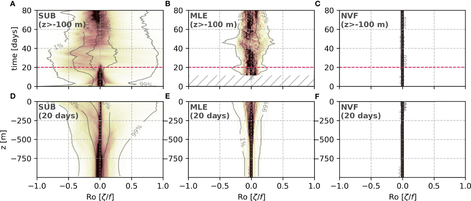
Figure 4 Time evolution (A–C) and day 20 vertical distribution (D–F) of the Rossby number for the different simulations.

Although there are slight differences, the MLE presents the same cross-front mixed layer depth patterns as the SUB experiment (Figure 5). Most of the mixed layer shoaling occurs between simulation days 13 and 30. The restratification process in the MLE differs from the SUB. The parameterization confines the higher stratification values in the top 20 m despite showing similar averaged mixed-layer depth after 40 days, whereas in the SUB, the top 200 m is restratifying. By definition, the NVF has the same averaged mixed-layer depth and stratification as SUB, since it is an SUB coarse-grained average.

FIGURE 5

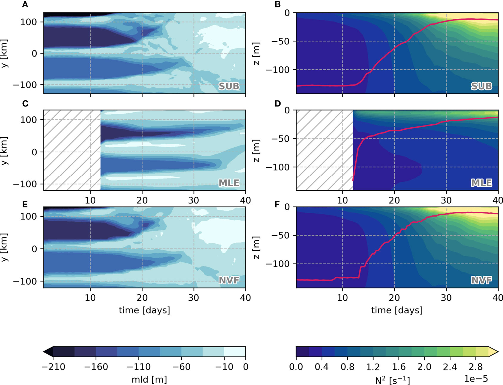
Figure 5 Time evolution of the average cross-front mixed-layer depth (A, C, E) and vertical profile of stratification (B, D, F) for each simulation. Red line is the average mixed-layer depth.

The differences between SUB and MLE occur because the parameterization restricts the submesoscale processes to the mixed layer. On the other hand, by imposing null vertical fluxes on the NVF, the bloom is weakened as the ecosystem reaches its maximum capacity, being sustained essentially by recycled production. However, our simulations demonstrate that submesoscale vertical velocities can reach depths far below the base of the mixed layer, enhancing the nitrate fluxes, particularly in weakly stratified waters, which agrees with other studies (e.g. Erickson et al., 2020).

5 Spring bloom

The biological response to the early-spring restratification usually manifests as an exponential growth of phytoplankton – the spring bloom – which saturates after depleting most of the mixed layer nutrients (Bagniewski et al., 2011). In our case, since there are no surface buoyancy fluxes, the restratification is driven solely by mixed layer eddies. If the restratification is the primary driver of the spring bloom, one should expect all simulations to have the same vertically-integrated average of new production. However, the bloom in SUB is more intense than in MLE and NVF, irrespective of the choice of μ (Figure 6), i.e., the vertical fluxes are also crucial for the new production dynamics, or the nutrient depletion would be reached earlier in the season, slowing down or interrupting the phytoplankton growth.

FIGURE 6

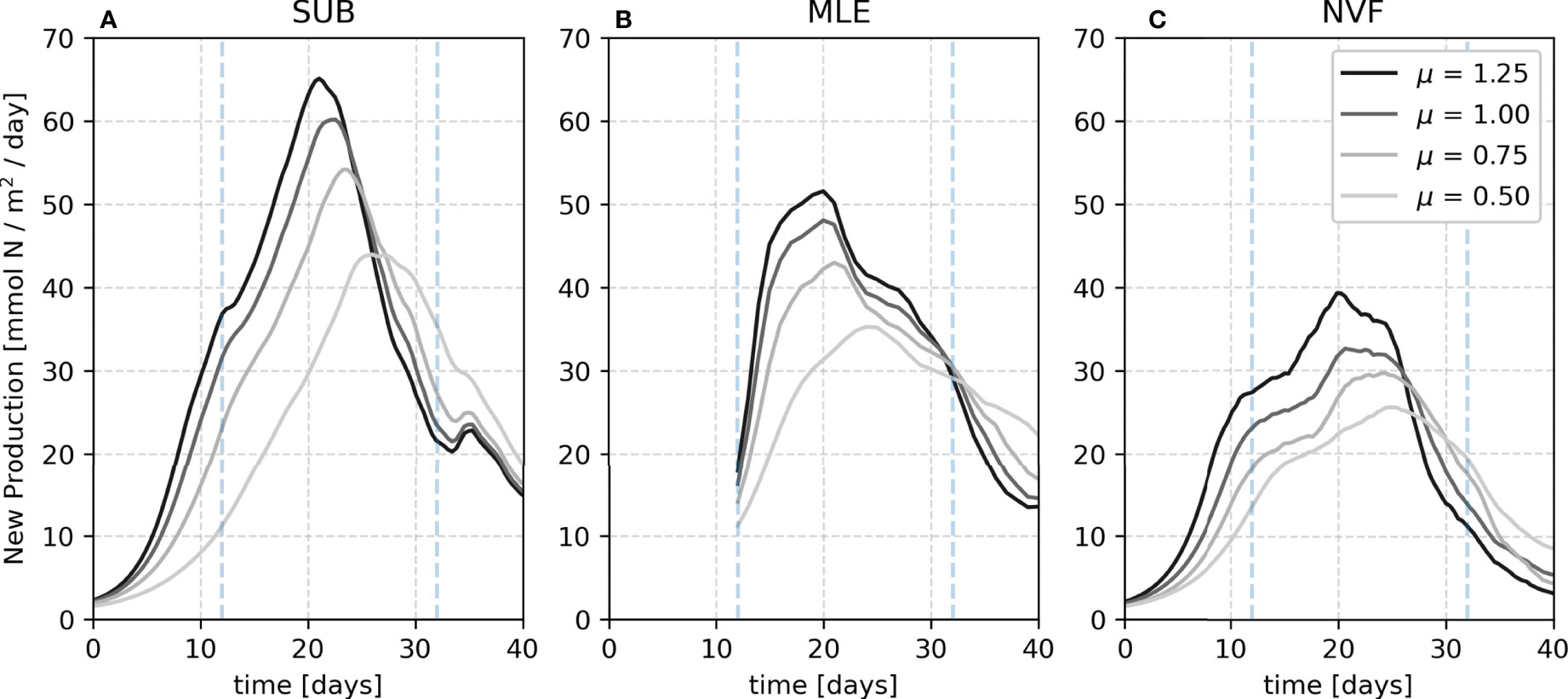
Figure 6 Vertically integrated average new production for SUB (A), MLE (B) and NVF (C) for each maximum growth rate of the phytoplankton (μ). Blue dashed lines represent the time range for the time integrated values presented in Table 1.

Among simulations, the peak of new production occurs between days 20 and 25, being progressively delayed with smaller μ values (Figure 6). We compare the total production between simulations from the beginning of the MLE and 20 days after (12–32 days, Table 1). The time range is chosen to capture the bulk of new production. Compared to the SUB, the time-integrated new production is 10-13.5% and 32.2-39.7% lower in the MLE and NVF, respectively, with smaller differences in the extreme μ values (0.5 and 1.25 day^-1). This dependence on the growth rate might be due to the timescale coupling between nutrient uptake by the phytoplankton and nutrient vertical fluxes (Freilich et al., 2022). We focus the rest of our analysis using μ= 0.75 day^-1.

TABLE 1

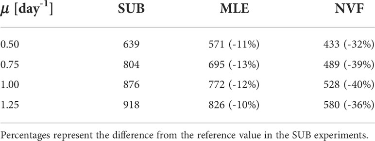
Table 1 Total new production [mmol N m²] from day 12 to 32.

In the real world, successive springtime storms could mix the upper ocean and generate new fronts that would then go unstable. Such processes are ignored in our experiments but, they could bring in extra nutrients. Nevertheless, the main purpose of our work is to address the importance of the submesoscale eddy-driven vertical fluxes of nutrients for the spring phytoplankton bloom.

The cross-front and vertical patterns of the new production are also different between experiments. The average cross-front new production is more laterally spread out for the SUB whereas confined to the restratification region in MLE and NVF (Figures 7A, C, E). The peak of new production occurs slightly deeper and later in SUB (20 m at day 22) than in MLE (15 m at day 17). The vertical distribution of the new production in NVF is a weaker version of SUB for the first 30 days, and then restricted to the mixed layer afterward (Figures 7B, D, F). This difference between 30 and 40 days is probably due to the higher lateral variability and patchiness of the mixed-layer depth in SUB compared to NVF.

FIGURE 7

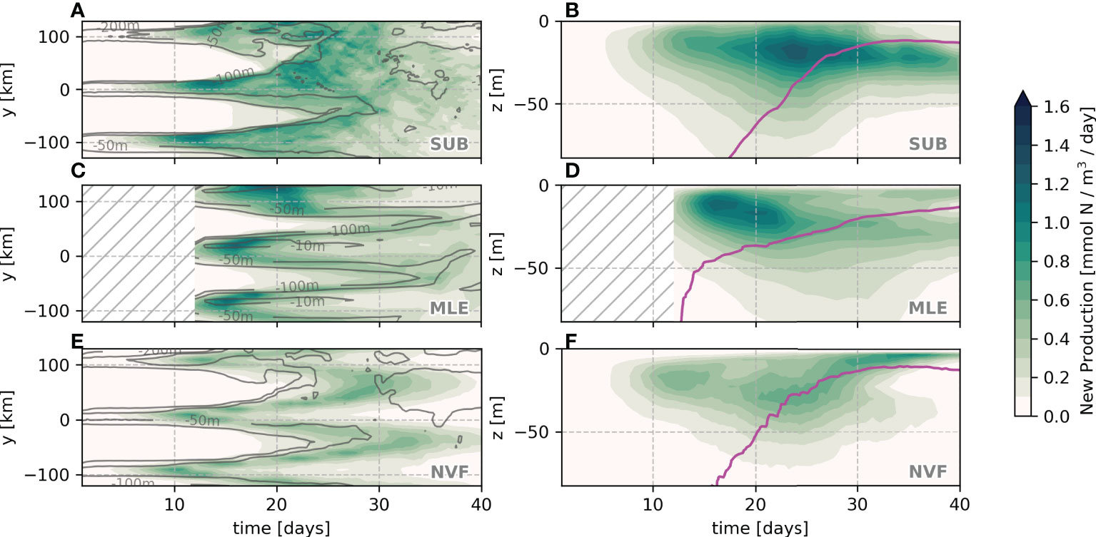
Figure 7 Average cross-front (A, C, E) and vertical profile (B, D, F) of new production for the first 70 m for μ=0.75 day^-1. Gray lines represent the zonally averaged mixed-layer depth and the magenta line represents the average mixed-layer depth.

6 Vertical nutrient fluxes

As mentioned previously, the major difference among the simulations is the vertical nutrient fluxes, partially solved and parameterized in the MLE and absent in the NVF experiments. Isopycnals, originally from the pycnocline, which outcrop in the mixed layer, can enhance the exchange between the interior pycnocline and the upper ocean. Unstable fronts and frontogenesis result in the enhancement of along-isopycnal vertical velocities (Freilich and Mahadevan, 2019). Accordingly, most of the nutrient flux in the SUB simulation occurs due to submesoscale dynamics, following sharp and strong fronts, i.e. strong vertical nutrient fluxes occur close to outcropping isopycnals at the base of the mixed layer (gray lines, Figures 8A, B). After 35 days, the velocity field is dominated by mesoscale features (Figures 3C, D) and the vertical fluxes are diminished, leading to a weak nutrient supply into the mixed layer (Figure 8A).

FIGURE 8

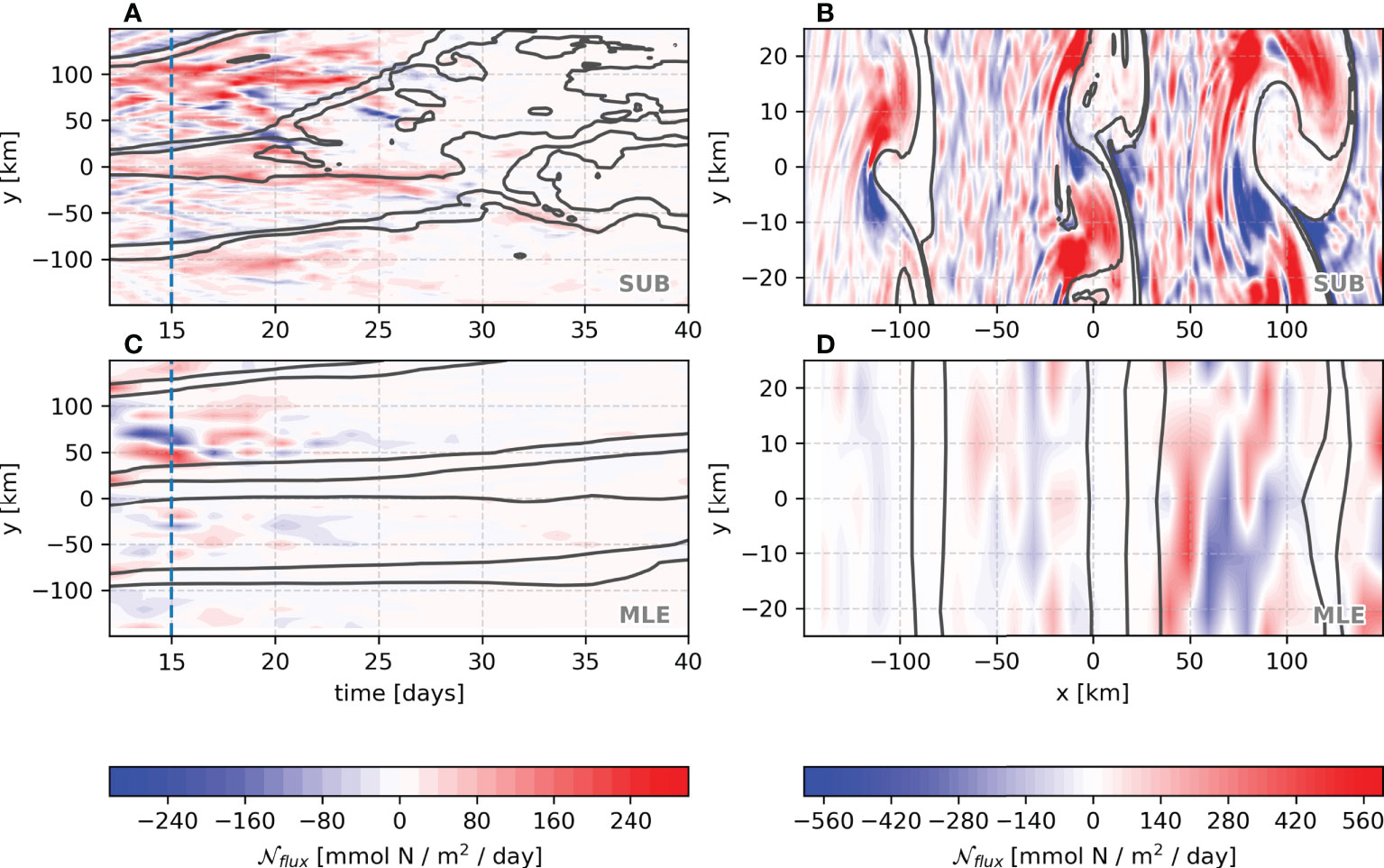
Figure 8 Vertical nitrate fluxes at the base of the mixed layer: average cross-front time evolution (A, C) and the day-15 snapshot (B, D) for SUB and MLE simulations. The gray solid lines mark isopycnal contours.

The MLE simulation shows both upward and downward nutrient fluxes, resulting in some cancellation, whereas, in the SUB, they are more positive into the mixed layer from pycnoclinic levels (Figures 8C, D). This leads to an order magnitude larger vertical nutrient flux in the SUB than in the MLE (Figures 9A, B). Furthermore, as expected from the vertical structure function (Equation 15), the MLE maximum vertical flux occurs in the middle of the mixed layer, while in SUB, it peaks close to the mixed layer base. The mean SUB nutrient flux peaks at day 17, remaining positive and mostly above 10 mmol N/m²/day up to the first 25 days of simulation (orange line, Figure 9C).

FIGURE 9

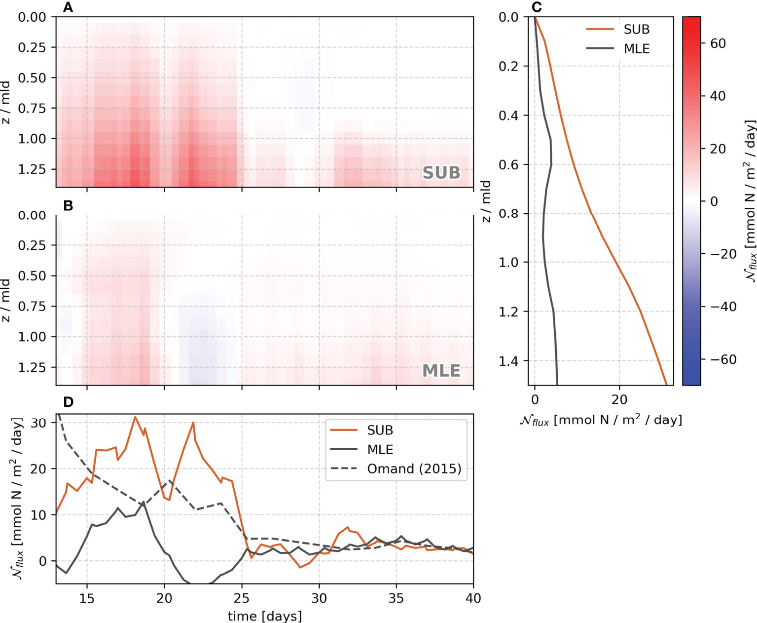
Figure 9 Average vertical profile of vertical nitrate fluxes for SUB (A) and MLE (B). The z coordinate is scaled by the local mixed-layer depth before the horizontal averaging. The average profile from 12 to 25 days is shown in panel (C) The time evolution of the vertical flux of nutrients at the base of the mixed layer (z/mld=1) is shown in panel (D) Orange lines represent SUB and gray lines for MLE. The gray dashed line represents the Omand et al. (2015) parameterization applied to MLE.

All these differences between the SUB and MLE imply that the mixed layer eddy parameterization does not reproduce the magnitude and vertical level of the maximum tracer flux, despite similar eddy-driven restratification being reproduced in both simulations. Alternatively, Omand et al. (2015) propose a parameterization for the vertical flux of an arbitrary tracer ( T ) across the mixed layer base as

$\begin{array}{ll}{T}_{flux}\approx \left|\overrightarrow{\text{Ψ}}\right|\frac{M^2}{N^2}\frac{\left[T\right]}{H},& (13)\end{array}$

where $\frac{M^2}{N^2}=\frac{\left|{\nabla }_{h}b\right|}{b_z}$ is the isopycnal slope in the restratifying region, and [T] is the tracer concentration right below the mixed layer. Compared to the SUB simulation, the Omand et al. (2015) parameterization applied to the MLE improves the magnitude and the decay of the nutrient fluxes after 25 days (dashed gray line, Figure 9C).

7 Discussion and concluding remarks

Submesoscale processes are essential for the vertical flux of nutrients in the upper ocean (Thomas et al., 2008; Mahadevan, 2016) and significantly affect the primary production in nutrient-limited seasons (Pasquero et al., 2005; Freilich and Mahadevan, 2019). Our numerical experiments evaluate the impact of submesoscale vertical nitrate fluxes on the spring bloom in the North Atlantic, which are not included in coarse resolution models even with mixed layer eddy parameterizations. On the other hand, these parameterizations are able to reproduce the shoaling of the mixed layer and bloom onset.

One caveat is the highly simplified ecosystem model employed with no representation of the phytoplankton community structure or higher trophic levels. We also ignore the vertical migration, plankton aggregation, and remineralization. In addition, the wind forcing could also play an important role since springtime storms could restore the fronts. In that case, the relaxation by the eddy-driven restratification will continue to occur between successive storms, inducing mixed layer shoaling and patchy nutrient fluxes, which we demonstrate to be an important process. The surface forcing coupled with submesoscale dynamics shows enhanced vertical mixing at the base of the mixed layer (Liu et al., 2021), which could lead to even higher vertical nutrient fluxes.

A comprehensive understanding of submesoscale processes in the upper ocean and, consequently, their parameterization is necessary to improve climate predictions. We show that the submesoscale motions are reaching deep, far below the base of the mixed layer, bringing extra nutrients into the euphotic zone. This mechanism is not reproduced by the current mixed layer eddy parameterizations, where the nutrient fluxes are maximum in the middle of the mixed layer. These results suggest that the climate models may underestimate the primary production in frontal systems. As a matter of fact, (Couespel et al., 2021) draw attention to the need for a better representation of the role of eddies in the nutrient fluxes below the mixed layer for more accurate comprehension of the future evolution of marine biomass. Moreover, submesoscale vertical motions tend to be weaker in late winter and springtime in future-climate scenarios for the North Atlantic (Richards et al., 2021) which calls for improved parameterizations for a more accurate representation of the carbon cycle in climate predictions.

We next put our study in context of previous work. Pasquero et al. (2005) described how the primary production is considerably affected by the temporal and spatial form of nutrient inputs. However, their vertical nutrient fluxes were externally imposed and ignored light limitation. Behrenfeld (2010) suggested that phytoplankton blooms are frequently initiated when the mixed layer depth is at its maximum. This idea relates the dilution of plankton in deep mixed layers to a reduced grazing and thus enhancing the phytoplankton growth. In our work, we simulate phytoplankton blooms akin to the one described in the North Atlantic Bloom 2008 experiment (Mahadevan et al., 2012), carried out during a period of eddy-driven shoaling mixed layers. Even considering the interannual variability, Erickson and Thompson (2018) show another north-Atlantic phytoplankton bloom following the shoaling of mixed layers (2012-2013), with shorter eddy-driven restratification events occurring in wintertime. They also highlight the importance of submesoscale instabilities for restratification and regional carbon export.

In the SUB simulation, the highest fluxes occur at the base of the mixed layer in regions of outcropping isopycnals (Figures 9A–D). Most of the previous studies on the springtime phytoplankton bloom in climate models consider the effect of the absence of mixed layer eddies, leading to a slower restratification. While this restratification is included via the mixed layer eddy parameterization (Fox-Kemper et al., 2011), the vertical fluxes approach zero at the base of the mixed layer. The Omand et al. (2015) parameterization performs better for the magnitude and decay presented by the mean nutrient flux at the base of the mixed layer as in the submesoscale-resolving simulation. Still, submesoscale fluxes do not necessarily decay exponentially in time as the Omand et al. (2015) parameterization suggests, and the application of this parameterization is restricted to the base of the mixed layer, and hence difficult to implement in three-dimensional models.

Despite reproducing a similar eddy-driven restratification from SUB simulation, the MLE simulation lacks most of the eddy-driven fluxes at the base of the mixed layer, which leads to a difference of 10–13% in the total springtime phytoplankton new production. Differences are even higher for the NVF simulation, showing that the eddy driven nutrient fluxes could be responsible for about 32–40% of the springtime phytoplankton new production.

Callies et al. (2016) discuss the penetration of mixed-layer eddies below the mixed layer. The eddies are initially restricted to the mixed layer, but by increasing their horizontal scale, they become more barotropic, following the expected character for geostrophic turbulence. The vertical decay of the eddy fluxes scale by k N/f, where k is the wavenumber, N the stratification right below the mixed layer and f the local planetary vorticity. This reveals that, for a weak stratification akin to the winter-to-spring transition in the North Atlantic, the eddies penetrate deeper as they grow (Erickson and Thompson, 2018, Figure 12). This is an important aspect that we confirm to be neglected by Fox-Kemper et al. (2011)’s parameterization. In other words, our analyses show that, in weakly stratified waters, mixed layer eddies bring extra nutrients from the base of the mixed layer and have an important role for the carbon uptake in subpolar oceans.

Data availability statement

The code for all simulations and analyses is available at the GitHub repository https://github.com/iuryt/NorthAtlanticBloom.

Author contributions

IS-S did the processing, modeling, and analyses and was the lead writer. AT and AM provided overall guidance contributing to the study formulation, interpretation of results, and writing of the paper. FP contributed to the definition of the initial conditions, formulation, and interpretation of the biogeochemical model, and the writing of the manuscript. CL contributed to the interpretation of the results and helped with writing the manuscript. All authors contributed to the article and approved the submitted version.

Funding

A.T. and A.M. thank, respectively, NSF-OCE-1755313 and NSF-OCE-1756279 for their support. This work started with support from NSF OCE 1434512 (A.T.), NSF OCE I434788 (A.M.) and ONR N00014-18-12799 (A.T. and I.T.S.). F.P. was supported by FAPESP (2017/15026-6 and 2021/08572-0).

Acknowledgments

IS-S thanks Gregory Wagner and Chris Hill for the precious help with the implementation of the biogeochemical and MLE parameterization on Oceananigans.jl. IS-S also thanks Glenn Flierl for the discussions on the biogeochemical formulation, Tilly Woods for the help with the mathematical notations, and Agata Piffer-Braga for the valuable discussions on the analyses.

Conflict of interest

The authors declare that the research was conducted in the absence of any commercial or financial relationships that could be construed as a potential conflict of interest.

Publisher’s note

All claims expressed in this article are solely those of the authors and do not necessarily represent those of their affiliated organizations, or those of the publisher, the editors and the reviewers. Any product that may be evaluated in this article, or claim that may be made by its manufacturer, is not guaranteed or endorsed by the publisher.

References

Álvarez E., Thoms S., Voelker C. (2018). Chlorophyll to carbon ratio derived from a global ecosystem model with photodamage. Global Biogeochem. Cycles 32, 799–816. doi: 10.1029/2017GB005850

CrossRef Full Text | Google Scholar

Argo (2020). Argo float data and metadata from global data assembly centre (Argo GDAC). doi: 10.17882/42182

CrossRef Full Text | Google Scholar

Badin G., Tandon A., Mahadevan A. (2011). Lateral mixing in the pycnocline by baroclinic mixed layer eddies. J. Phys. Oceanogr. 41, 2080–2101. doi: 10.1175/JPO-D-11-05.1

CrossRef Full Text | Google Scholar

Bagniewski W., Fennel K., Perry M. J., D’Asaro E. A. (2011). Optimizing models of the north Atlantic spring bloom using physical, chemical and bio-optical observations from a Lagrangian float. Biogeosciences 8, 1291–1307. doi: 10.5194/bg-8-1291-2011

CrossRef Full Text | Google Scholar

Behrenfeld M. J. (2010). Abandoning sverdrup’s critical depth hypothesis on phytoplankton blooms. Ecology 91, 977–989. doi: 10.1890/09-1207.1

PubMed Abstract | CrossRef Full Text | Google Scholar

Behrenfeld M. J., Boss E. S. (2014). Resurrecting the ecological underpinnings of ocean plankton blooms. Annu. Rev. Mar. Sci. 6, 167–194. doi: 10.1146/annurev-marine-052913-021325

CrossRef Full Text | Google Scholar

Callies J., Flierl G., Ferrari R., Fox-Kemper B. (2016). The role of mixed-layer instabilities in submesoscale turbulence. J. Fluid Mechanics 788, 5–41. doi: 10.1017/jfm.2015.700

CrossRef Full Text | Google Scholar

Couespel D., Lévy M., Bopp L. (2021). Oceanic primary production decline halved in eddy-resolving simulations of global warming. Biogeosciences 18, 4321–4349. doi: 10.5194/bg-18-4321-2021

CrossRef Full Text | Google Scholar

Diaz B. P., Knowles B., Johns C. T., Laber C. P., Bondoc K. G. V., Haramaty L., et al. (2021). Seasonal mixed layer depth shapes phytoplankton physiology, viral production, and accumulation in the north Atlantic. Nat. Commun. 12, 1–16. doi: 10.1038/s41467-021-26836-1

PubMed Abstract | CrossRef Full Text | Google Scholar

Erickson Z. K., Thompson A. F. (2018). The seasonality of physically driven export at submesoscales in the northeast atlantic ocean. Global Biogeochem. Cycles 32, 1144–1162. doi: 10.1029/2018GB005927

CrossRef Full Text | Google Scholar

Erickson Z. K., Thompson A. F., Callies J., Yu X., Garabato A. N., Klein P. (2020). The vertical structure of open-ocean submesoscale variability during a full seasonal cycle. J. Phys. Oceanogr. 50, 145–160. doi: 10.1175/JPO-D-19-0030.1

CrossRef Full Text | Google Scholar

Fasham M. J., Ducklow H. W., McKelvie S. M. (1990). A nitrogen-based model of plankton dynamics in the oceanic mixed layer. J. Mar. Res. 48, 591–639. doi: 10.1357/002224090784984678

CrossRef Full Text | Google Scholar

Fox-Kemper B., Danabasoglu G., Ferrari R., Griffies S., Hallberg R., Holland M., et al. (2011). Parameterization of mixed layer eddies. iii: Implementation and impact in global ocean climate simulations. Ocean Model. 39, 61–78. doi: 10.1016/j.ocemod.2010.09.002

CrossRef Full Text | Google Scholar

Fox-Kemper B., Ferrari R. (2008). Parameterization of mixed layer eddies. part ii: Prognosis and impact. J. Phys. Oceanogr. 38, 1166–1179. doi: 10.1175/2007JPO3788.1

CrossRef Full Text | Google Scholar

Fox-Kemper B., Ferrari R., Hallberg R. (2008). Parameterization of mixed layer eddies. part i: Theory and diagnosis. J. Phys. Oceanogr. 38, 1145–1165. doi: 10.1175/2007JPO3792.1

CrossRef Full Text | Google Scholar

Freilich M. A., Flierl G. R., Mahadevan A. (2022). Diversity of growth rates maximizes phytoplankton productivity in an eddying ocean. Geophys. Res. Lett. 49, e2021GL096180. doi: 10.1029/2021GL096180

CrossRef Full Text | Google Scholar

Freilich M. A., Mahadevan A. (2019). Decomposition of vertical velocity for nutrient transport in the upper ocean. J. Phys. Oceanogr. 49, 1561–1575. doi: 10.1175/JPO-D-19-0002.1

CrossRef Full Text | Google Scholar

Freilich M., Mignot A., Flierl G. R., Ferrari R. (2021). Grazing behavior and winter phytoplankton accumulation. Biogeosciences 18, 5595–5607. doi: 10.5194/bg-18-5595-2021

CrossRef Full Text | Google Scholar

Garcia H. E., Weathers K., Paver C. R., Smolyar I. V., Boyer T. P., Locarnini R. A., et al. (2018). World ocean atlas 2018, volume 4: Dissolved inorganic nutrients (phosphate, nitrate and nitrate+nitrite, silicate). a. v. mishonov, technical Editor. NOAA Atlas NESDIS 84, 35pp. Available at: https://archimer.ifremer.fr/doc/00651/76336/

Google Scholar

Gruber N., Frenzel H., Doney S. C., Marchesiello P., McWilliams J. C., Moisan J. R., et al. (2006). Eddy-resolving simulation of plankton ecosystem dynamics in the California current system. Deep Sea Res. Part I: Oceanogr. Res. Papers 53, 1483–1516. doi: 10.1016/j.dsr.2006.06.005

CrossRef Full Text | Google Scholar

Karimpour F., Tandon A., Mahadevan A. (2018). Sustenance of phytoplankton in the subpolar north atlantic during winter. J. Geophys. Res.: Oceans 123, 6531–6548. doi: 10.1029/2017JC013639

CrossRef Full Text | Google Scholar

Lachkar Z., Gruber N. (2011). What controls biological production in coastal upwelling systems? insights from a comparative modeling study. Biogeosciences 8, 2961–2976. doi: 10.5194/bg-8-2961-2011

CrossRef Full Text | Google Scholar

Lévy M., Franks P. J., Smith K. S. (2018). The role of submesoscale currents in structuring marine ecosystems. Nat. Commun. 9, 1–16. doi: 10.1038/s41467-018-07059-3

PubMed Abstract | CrossRef Full Text | Google Scholar

Liu G., Bracco A., Sitar A. (2021). Submesoscale Mixing Across the Mixed Layer in the Gulf of Mexico. Frontiers in Marine Science, 8, 615066. doi: 10.3389/fmars.2021.615066

CrossRef Full Text | Google Scholar

Mahadevan A. (2016). The impact of submesoscale physics on primary productivity of plankton. Annu. Rev. Mar. Sci. 8, 161–184. doi: 10.1146/annurev-marine-010814-015912

CrossRef Full Text | Google Scholar

Mahadevan A., D’asaro E., Lee C., Perry M. J. (2012). Eddy-driven stratification initiates north atlantic spring phytoplankton blooms. Science 337, 54–58. doi: 10.1126/science.1218740

PubMed Abstract | CrossRef Full Text | Google Scholar

Mahadevan A., Tandon A., Ferrari R. (2010). Rapid changes in mixed layer stratification driven by submesoscale instabilities and winds. J. Geophys. Res.: Oceans 115, C03017. doi: 10.1029/2008JC005203

CrossRef Full Text | Google Scholar

Marshall J., Adcroft A., Hill C., Perelman L., Heisey C. (1997). A finite-volume, incompressible navier stokes model for studies of the ocean on parallel computers. J. Geophys. Res.: Oceans 102, 5753–5766. doi: 10.1029/96JC02775

CrossRef Full Text | Google Scholar

Martinez E., Antoine D., d’Ortenzio F., de Boyer Montégut C. (2011). Phytoplankton spring and fall blooms in the north Atlantic in the 1980s and 2000s. J. Geophys. Res.: Oceans 116, C11029. doi: 10.1029/2010JC006836

CrossRef Full Text | Google Scholar

McWilliams J. C. (2016). Submesoscale currents in the ocean. Proc. R. Soc. A: Mathematical Phys. Eng. Sci. 472, 20160117. doi: 10.1098/rspa.2016.0117

CrossRef Full Text | Google Scholar

Omand M. M., D’Asaro E. A., Lee C. M., Perry M. J., Briggs N., Cetinić I., et al. (2015). Eddy-driven subduction exports particulate organic carbon from the spring bloom. Science 348, 222–225. doi: 10.1126/science.1260062

PubMed Abstract | CrossRef Full Text | Google Scholar

Oschlies A. (2002). Improved representation of upper-ocean dynamics and mixed layer depths in a model of the north Atlantic on switching from eddy-permitting to eddy-resolving grid resolution. J. Phys. Oceanogr. 32, 2277–2298. doi: 10.1175/1520-0485(2002)032<2277:IROUOD>2.0.CO;2

CrossRef Full Text | Google Scholar

Pasquero C., Bracco A., Provenzale A. (2005). Impact of the spatiotemporal variability of the nutrient flux on primary productivity in the ocean. J. Geophys. Res.: Oceans 110, C07005. doi: 10.1029/2004JC002738

CrossRef Full Text | Google Scholar

Ramadhan A., Wagner G. L., Hill C., Campin J.-M., Churavy V., Besard T., et al. (2020). Oceananigans.jl: Fast and friendly geophysical fluid dynamics on GPUs. J. Open Source Softw. 5, 2018. doi: 10.21105/joss.02018

CrossRef Full Text | Google Scholar

Richards K. J., Whitt D. B., Brett G., Bryan F. O., Feloy K., Long M. C. (2021). The impact of climate change on ocean submesoscale activity. J. Geophys. Res.: Oceans 126, e2020JC016750. doi: 10.1029/2020JC016750

CrossRef Full Text | Google Scholar

Sarmiento J.L., Slater R.D., Fasham M.J.R., Ducklow H.W., Toggweiler J.R., Evans G.T. (1993) A seasonal three‐dimensional ecosystem model of nitrogen cycling in the North Atlantic euphotic zone. Global biogeochemical cycles, 7 (2), 417–450. doi: 10.1029/93GB00375

CrossRef Full Text | Google Scholar

Sverdrup H. U. (1953). On conditions for the vernal blooming of phytoplankton. ICES J. Mar. Sci. 18, 287–295. doi: 10.1093/icesjms/18.3.287

CrossRef Full Text | Google Scholar

Takahashi T., Sutherland S. C., Wanninkhof R., Sweeney C., Feely R. A., Chipman D. W., et al. (2009). Climatological mean and decadal change in surface ocean pCO2, and net sea–air CO2 flux over the global oceans. Deep Sea Res. Part II: Topical Stud. Oceanogr. 56, 554–577. doi: 10.1016/j.dsr2.2008.12.009. Surface Ocean CO2 Variability and Vulnerabilities.

CrossRef Full Text | Google Scholar

Taylor J. R., Ferrari R. (2011). Ocean fronts trigger high latitude phytoplankton blooms. Geophys. Res. Lett. 38, L23601. doi: 10.1029/2011GL049312

CrossRef Full Text | Google Scholar

Thomas L. N., Tandon A., Mahadevan A. (2008). Submesoscale Processes and Dynamics. In Ocean Modeling in an Eddying Regime (eds M.W. Hecht and H. Hasumi). doi: 10.1029/177GM04

CrossRef Full Text | Google Scholar

Thomas L. N., Taylor J. R., Ferrari R., Joyce T. M. (2013). Symmetric instability in the gulf stream. Deep Sea Res. Part II: Topical Stud. Oceanogr. 91, 96–110. doi: 10.1016/j.dsr2.2013.02.025

CrossRef Full Text | Google Scholar