 Bayoumy Mohamed
 Frank Nilsen
 Ragnheid Skogseth
94% of researchers rate our articles as excellent or good
Learn more about the work of our research integrity team to safeguard the quality of each article we publish.
Find out more
ORIGINAL RESEARCH article
Front. Mar. Sci., 16 March 2022
Sec. Physical Oceanography
Volume 9 - 2022 | https://doi.org/10.3389/fmars.2022.821646
Marine heatwaves (MHWs) can potentially alter ocean ecosystems with far-reaching ecological and socio-economic consequences. This study investigates the spatiotemporal evolution of the main MHW characteristics in the Barents Sea using high-resolution (0.25° × 0.25°) daily Sea Surface Temperature (SST) data from 1982 to 2020. The results reveal that the Barents Sea has experienced accelerated warming and several more MHWs in recent decades. Since 2004, an amplified increasing SST trend was observed across the entire Barents Sea, with a spatially averaged SST trend of 0.25 ± 0.18°C/decade and 0.58 ± 0.21°C/decade for the northern and southern Barents Sea, respectively. The annual mean MHW frequency, days, and duration over the entire Barents Sea increased by, respectively, 62, 73, and 31% from the pre- to the post-2004 period. More than half of all MHW days occurred in the last decade (2011–2020). The most intense MHW event occurred in summer 2016, which was also the warmest year during the study period. In general, the annual mean MHW frequency was relatively high in the northern Barents Sea, while the intensity and duration were higher in the southern Barents Sea. The highest annual MHW intensity and duration were observed in 2016, 2013, and 2020, respectively, while the highest annual MHW frequency was found in 2016. For the entire Barents Sea, the annual MHW frequency and duration increased significantly (p < 0.05) over the whole study period, with a trend of, respectively, 1.0 ± 0.4 events/decade, which is a doubling of the global average, and 2.4 ± 1.3 days/decade. In terms of the influence of climate variability on MHW characteristics, our findings revealed that the Eastern Atlantic Pattern (EAP) plays a significant role in controlling MHW characteristics, whereas the North Atlantic Oscillation (NAO) has no significant relationship. Sea ice concentrations were found to have a significant negative correlation with MHW characteristics. Strong positive correlations were observed between SST, surface air temperature, and MHW frequency, implying that as global warming continues, we can expect continued rising in MHW frequencies and days in the Barents Sea with huge implications for the ocean ecosystem.
Marine heatwaves (MHWs) have become one of the major concerns and a hot topic in climate change research in recent decades (Marx et al., 2021) due to their destructive impact on marine biodiversity, ecosystems, and fisheries (Selig et al., 2010; Mills et al., 2013; Frölicher and Laufkötter, 2018; Li et al., 2019; Smale et al., 2019). Marine species react to MHWs by shifting their geographic distribution and hence, affecting fisheries that target those species (Mills et al., 2013). Severe MHWs have been occurring around the world in recent decades (Hobday et al., 2016; Oliver et al., 2018), for example, in the northern Mediterranean Sea in 2003 (Olita et al., 2007; Ibrahim et al., 2021), offshore of Western Australia in 2010/2011 (Pearce and Feng, 2013), in the northwest Atlantic in 2012 (Chen et al., 2014), in the northeast Pacific over 2013–2015 (Di Lorenzo and Mantua, 2016), in the Tasman Sea in 2015/2016 (Oliver et al., 2017), across northern Australia in 2016 (Benthuysen et al., 2018), in the southwestern Atlantic Shelf in 2017 (Manta et al., 2018), in the China Seas in 2017 (Li et al., 2019), and over the Red Sea in 2019 (Mohamed et al., 2021). These extreme MHW events are leading to environmental and socio-economic impacts, including widespread coral bleaching (Hughes et al., 2017), benthic invertebrate mortality (Garrabou et al., 2009), harmful algal blooms (Trainer et al., 2020), reduced levels of surface chlorophyll (Bond et al., 2015), loss of seagrass meadows and kelp forests (Arias-Ortiz et al., 2018; Thomsen et al., 2019), and changes in fishing practices and increased economic tensions between countries (Mills et al., 2013).
The most recent definition of a MHW is an anomalously warm water event that persists (at least five consecutive days) with temperatures above a seasonally varying threshold (Hobday et al., 2016, 2018). MHWs can be classified based on several factors, including frequency, duration, and intensity. According to recent studies, the global average annual MHW frequency and duration have increased by 34 and 17%, respectively, resulting in a more than 50% increase in annual MHW days over the last century (Oliver et al., 2018). MHWs can be triggered by both-large scale and regional atmospheric- or oceanic processes, or by a combination of them. The most common cause of a MHW is heat advection by ocean currents that can build up areas of warm water (Oliver et al., 2017), or atmospheric overheating through an anomalous air-sea heat flux (Olita et al., 2007; Chen et al., 2015). Winds can either enhance or suppress warming during a MHW event (Garrabou et al., 2009), and large-scale atmospheric and oceanic teleconnection patterns can influence the likelihood of a MHW occurring in specific regions (Holbrook et al., 2019). In the North Atlantic and European regions, the North Atlantic Oscillation (NAO) is the most influential large-scale mode of SST and atmospheric variability (Scannell et al., 2016). During its strong positive phases, westerly winds are anomalously strong (Chafik et al., 2017), resulting in more intense storms and higher-than-average air temperatures in northern Europe, increasing the possibility of MHWs in this region. For example, Kueh and Lin (2020) attributed the 2018 summer MHW over northwestern Europe to the strongly positive phase of the NAO. Oliver (2019) discovered that, in most parts of the world’s ocean, the increase in mean SST, rather than its variability, has been the dominant driver of changes in MHW characteristics over the last decades. Moreover, as a result of global warming, MHWs are expected to become more frequent and intense over the next century (Frölicher et al., 2018). The warming rate in the Arctic region, particularly in the Barents Sea, has been nearly twice as fast as the global average in recent decades, a phenomenon known as “Arctic SST amplification” (Screen and Simmonds, 2010; Serreze and Barry, 2011; Schlichtholz, 2019; Hu et al., 2020). The ocean surface in the Barents Sea is a climate change hotspot (Lind et al., 2018; Schlichtholz, 2019) and hence, it is likely to see an increase in the number of MHW events in this region.
Over the satellite era, extensive work has been conducted on the SST warming rate and ice reduction in the Barents Sea. Barton et al. (2018) revealed a significant positive SST trend (up to 0.05°C/year) in the western Barents Sea during 1985–2004, while the eastern Barents Sea experienced the same trend the following decade from 2005 to 2016, which were consistent with the study by Herbaut et al. (2015). Lind et al. (2018) reported a significant linear trend in the upper 100 m temperature and ocean heat content over the Barents Sea from 2000 to 2016, while a non-significant trend was observed from 1970 to 1999. Observations document an approximate 50% decline in the winter sea-ice extent in the Barents Sea over the past four decades (Årthun et al., 2012; Onarheim et al., 2015). Variability in the sea-ice cover on interannual and longer time scales has been shown to be governed by oceanic heat transport (Årthun et al., 2012; Onarheim et al., 2015; Lien et al., 2017). The major transformation from warm Atlantic Water (AW) into colder Barents Sea Water (BSW) takes place along the throughflow branch from the southwestern Barents Sea to the outflow between Novaya Zemlya and Franz Joseph Land (see Figure 1) in the northeast (Schauer et al., 2002). Lien et al. (2017) provide a mechanistic understanding of the response of sea ice to ocean throughflow heat anomalies modulated by changes in volume transport, which is sensitive to both local and regional atmospheric forcing. Furthermore, Asbjørnsen et al. (2020) investigated the mechanism of recent Arctic “Atlantification” and discovered that the highest warming trends occurred south of the winter (March) ice edge, with ocean advection acting as the primary driver. Using observational and reanalysis data from 1987 to 2017, Skogseth et al. (2020) investigated the variability and trends of the ocean climate and circulation in Isfjorden, an Arctic fjord facing inflow of AW from the ocean west of Svalbard in the northwestern corner of the Barents Sea (Figure 1). They identified a climate shift in this region in 2006 and discovered a highly significant positive trend in mean summer (July–September) and winter (January–May) SST with a value of about 0.07 ± 0.01°C/year which they associated with increased inflow of AW higher up in the water column.
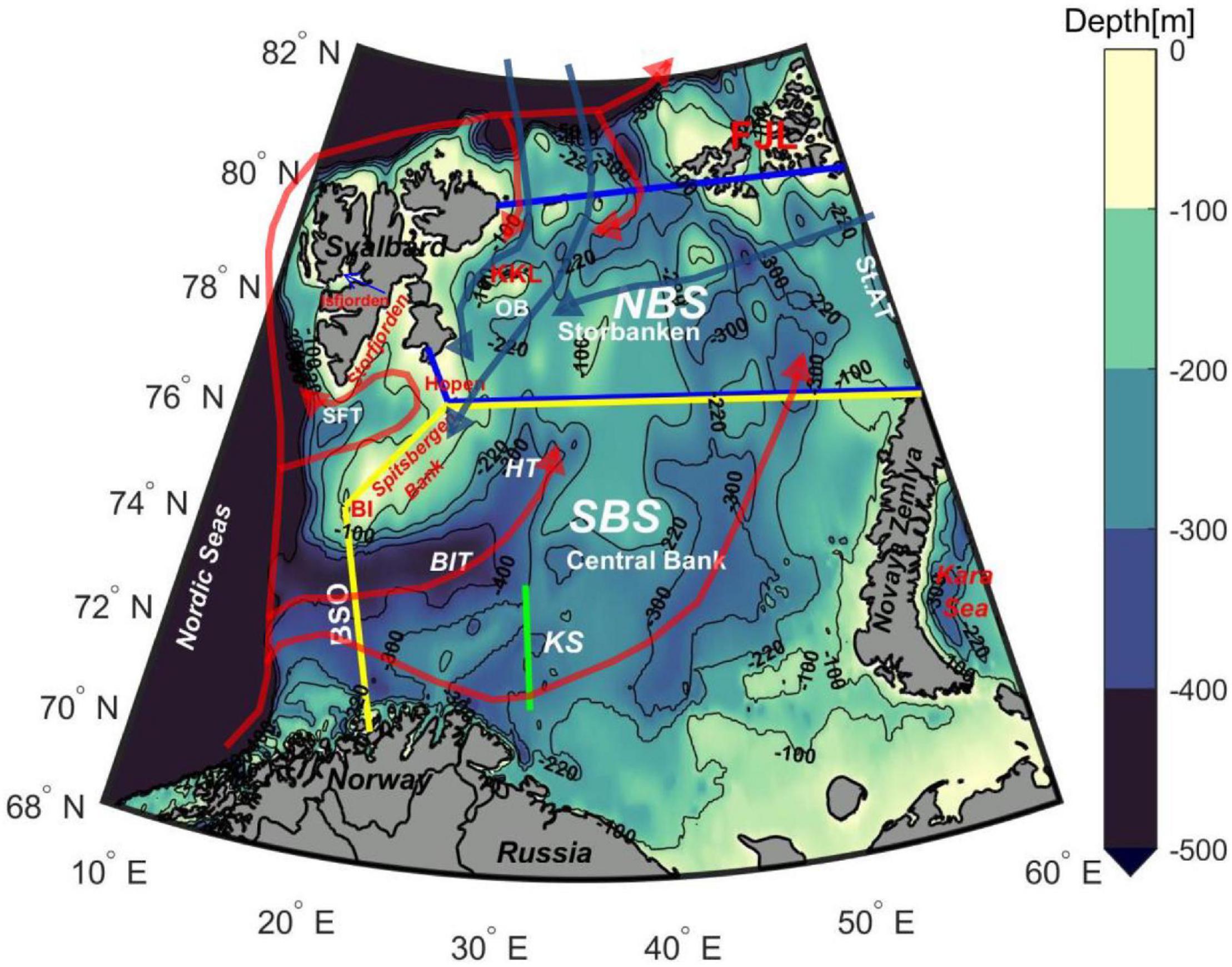
Figure 1. Bathymetric map of the study area with main geographical features. Bathymetric data obtained from a global 30 arc-second interval grid (GEBCO, https://www.gebco.net) with 10 m as the minimum depth. The Barents Sea was divided into two regions: northern Barents Sea (NBS, area inside the solid blue line), and southern Barents Sea (SBS, area inside the solid yellow lines). Red arrows show Atlantic water currents, blue arrows show Arctic water currents. Isobaths of 100, 220, 300, and 500 m are shown in black. The abbreviations stand for the Barents Sea Opening (BSO), Bear Island Trough (BIT), Hopen Trench (HT), Bear Island (BI), Storfjorden Trough (SFT), Kong Karls Land (KKL), Olga Basin (OB), Franz Joseph Land (FJL), and the St. Anna Trough (St.AT). The Kola Section (KS) is marked with straight green line.
Recently, Skagseth et al. (2020) have reported a reduced efficiency of “the Barents Sea cooling machine.” The Barents Sea cooling machine let all the heat from the inflowing AW escape to the atmosphere before entering the Arctic Ocean. When increased heat from inflowing AW extends the Atlantic domain downstream and reduces the winter sea ice cover, an increased heat loss to a cold enough atmosphere compensates for this increased inflow of warm AW locally where sea ice has retreated. Using hydrographic observations from 1971 to 2018, Skagseth et al. (2020) found evidence that the Barents Sea has changed to the extent that the cooling machine is weakening, and the present change is dominated by reduced ocean heat loss over the southern Barents Sea due to anomalous southerly winds bringing in warmer air masses. A warmer ocean surface layer and hence, an increased SST compared to a climatological mean is expected when the AW throughflow retains more of its initial and upstream heat content.
The Barents Sea is a region of great geopolitical and economic importance, including transportation, fishing, and military purposes, as well as the world’s fifth-largest deposit of oil and gas. The Barents Sea is a highly productive ecosystem, accounting for roughly 40% of the total Arctic shelves primary production (Oziel et al., 2017), with a diverse community of plankton that supports higher trophic levels (Dalpadado et al., 2012) including one of the world’s largest concentrations of seabirds and a diverse assemblage of marine mammals (Hunt et al., 2013), as well as some of the world’s largest stocks of cod, capelin, and haddock (Olsen et al., 2010). The Barents Sea is also the primary nursery ground for a large stock of Norwegian spring-spawning herring (Clupea harengus) (Dalpadado et al., 2014). However, as far as the authors know, there are no published studies on MHWs in the Barents Sea, except for the study by Hu et al. (2020) who found that MHWs in the entire Arctic region over the period 1988–2017 have become more frequent and intense in areas with varying sea ice cover (first and multiyear ice zones).
The main goal of this study is to provide a comprehensive analysis of SST change and the spatial-temporal evolution of MHW characteristics in the Barents Sea from 1982 to 2020, based on a high-resolution (0.25° × 0.25°) global daily SST dataset derived from satellites. Furthermore, we will investigate the influences and feedbacks between the recorded MHWs and two climate indices and three climate variables, including the North Atlantic Oscillation (NAO), Eastern Atlantic Pattern (EAP), Sea Surface Temperature (SST), Surface Air Temperature (SAT), and Sea Ice Concentration (SIC). These three climate variables have been identified as Essential Climate Variables (ECVs) by the Global Climate Observing System (GCOS) based on their climate relevance, technical feasibility, and cost-effectiveness (Bojinski et al., 2014), as they play an important role in regulating Earth’s climate system and its variability. Then, we will examine the relationship between the strong MHW event in 2016 and various atmospheric conditions such as SAT, wind speed, and sea level pressure.
The Barents Sea (BS) is a seasonally ice-covered shelf sea between the deep Norwegian Sea and Arctic Ocean basins between latitudes 68 and 80°N (Figure 1), connecting the warm Atlantic to the cold Arctic Ocean. The Barents Sea is bounded to the east by Novaya Zemlya Archipelago, to the northeast by Franz Josef Land, and to the northwest by the Svalbard Archipelago. The average depth of the Barents Sea is about 230 meters, with a maximum depth of about 300 meters, and the shallowest depth (<100 meters) on the Spitsbergen Bank (between Bear Island in the southwest and Hopen in the northeast). The Barents Sea is divided into two regions: the northern (Arctic) Barents Sea (NBS; area inside the blue lines) and the southern (Atlantic) Barents Sea (SBS; area inside the red lines), as shown in Figure 1. The SBS is strongly influenced by the inflow of warm AW, the largest oceanic heat source to the Barents Sea, while the NBS is controlled by colder Arctic Water (ArW) and has a more layered structure with the influence of seasonal sea ice formation and melt (Lind et al., 2018). The upper layer consists of relatively fresh ArW, while warm AW or cold dense water prevails near the bottom. The AW inflow enters from the southwestern Barents Sea through the Barents Sea Opening (BSO in Figure 1) and is predominantly barotropic (AW at the surface), with large fluctuations in both current speed and lateral structure (Ingvaldsen et al., 2002, 2004). The warm and saline AW flows northward following two main pathways (Figure 1): one going east into the Central Basin before turning north and eventually exiting through the St. Anna Trough and one shorter pathway turning north along the Hopen Trench (Loeng, 1991). The sea ice extent in winter is partly determined by the transition zone between the Atlantic and Arctic water masses, often termed the Polar Front. The Polar Front is topographically controlled and therefore rather stable in the west, closely following the 220-m isobath (Barton et al., 2018), where the thermal and haline gradient is oriented perpendicular to the direction of the flow. To the northeast, the thermal gradient is oriented along the flow of Atlantic Water because of stronger heat loss to the atmosphere and hence, a positive oceanic volume transport anomaly will cause a coherent ocean temperature increase (Chafik et al., 2015).
The daily SST data used in this study were obtained from the National Oceanic and Atmospheric Administration’s Optimum Interpolation Sea Surface Temperature version 2.1 [NOAA OISST V2.1; website1; Reynolds et al. (2007)]. OISST is a global high resolution (0.25° × 0.25°) daily SST product created by combining observations from various platforms (satellite, ships, and buoys) to produce a daily gap-free product (Banzon et al., 2016). The analysis data set includes both in situ data and large-scale adjustments and corrections of satellite biases. The new version (OISST V2.1) includes significant enhancements in Arctic regions (Huang et al., 2021a), which combines in situ and bias-corrected advanced very high-resolution radiometer (AVHRR) SST measurements. The AVHRR SSTs were adjusted to the buoy SSTs at the nominal depth of 0.2 m. The proxy SSTs derived from SIC (Banzon et al., 2020) were combined with other in situ and AVHRR SSTs in ice-covered regions when available. Furthermore, the warm SSTs bias in the Arctic regions was minimized by utilizing a freezing point rather than a regressed ice-SST proxy, which was produced by an inaccurate technique for estimating SST by proxy from SIC (Banzon et al., 2020). This dataset was used to extract the sea ice concentration at the same spatial and temporal resolution. The Barents Sea OISST data were extracted from the global data, yielding a 9860-point regularly gridded dataset spanning 14,245 days from 1 January 1982 to 31 December 2020.
Hourly gridded (0.25° × 0.25°) atmospheric variables were obtained from the European Centre for Medium-Range Weather Forecasts (ECMWF) ERA5 dataset (Hersbach et al., 2020). We used wind speed (U) and its components at ten meters height (u10 and v10), air temperature at two meters height (SAT, hereafter), and mean sea level pressure from 1982 to 2020. The Copernicus Climate Change Service Climate Data Store now hosts the fifth generation of ECMWF atmospheric reanalysis data2. Finally, the normalized time series of the North Atlantic Oscillation (NAO) and the East Atlantic Pattern (EAP) were obtained from the NOAA Climate Prediction Centre3.
Several techniques are used to define/calculate marine heatwaves (MHWs), including utilizing fixed, relative, or seasonally varying thresholds, and each has advantages and disadvantages. In this paper, we follows the standard MHW definition proposed by Hobday et al. (2016), which is “an abnormally warm water event that lasts at least 5 days with SST above the seasonally varying 90th percentile threshold for that time of year.” According to Hobday et al. (2016), the baseline SST climatology should be based on at least 30-year of data. The climatological mean and the 90th percentile threshold are calculated at each grid cell for each calendar day of the year using daily SST data over a 39-year historical baseline period (1982–2020). Two consecutive MHW events with a gap of 2 days or less are considered a single event. The daily varying threshold allows for the detection of MHW events at any time of the year, whereas fixed thresholds (e.g., Frölicher et al., 2018) typically only identify warm-season MHWs. Hobday is the most popular and commonly used MHW detection technique, as MHWs in colder months are critical for various biological applications. Each MHW event is described by a set of metrics (Hobday et al., 2016, 2018) which are as follows: duration (in days) is the time between the start and end dates of an event, frequency (in events) is the number of events that occurred in each year, mean intensity (°C) is the average SST anomaly (SSTA) over the duration of the event, cumulative intensity (°C days) is the integrated SSTA over the duration of the event, maximum intensity (°C) is the highest SSTA during an event, and days are the sum of MHW days in each year. SSTAs were estimated relative to the daily climatology.
The MATLAB toolbox M_MHW (4 Zhao and Marin, 2019) is used to detect all the MHW characteristics. Annual statistics and time series for MHW frequency, duration, and cumulative intensity are computed from 1982 to 2020 for each region (NBS and SBS, Figure 1). Linear trends in SSTA and MHW characteristics are estimated using the least-squares method (Wilks, 2011), and their statistical significance is determined using the Modified Mann–Kendall (MMK) test at a 95% confidence level (Hamed and Ramachandra Rao, 1998; Wang et al., 2020). Based on the observed climate shift in 2004 (Figure 2), we divided the dataset into two distinct periods: the cold period from 1982 to 2003 (pre-2004), with average temperatures below the 1982–2020 climatological mean, and the warm period from 2004 to 2020 (post-2004), with average temperatures above the 1982–2020 climatological mean. The spatial SSTA trend is then computed for each period. To assess the statistical significance of the recent changes in the mean MHW main characteristics between the pre-and post-2004, the usual two-sample Student t-test is employed (von Storch and Zwiers, 1999). The annual and seasonal temporal variations of these MHW characteristics are correlated with essential climate variables and teleconnection patterns such as SST, SIC, SAT, EAP, and NAO to better understand the relationship between MHW and atmospheric-oceanic connection. Here, we defined the summer season as (June–August) and the winter season as (December–February) to follow the previous study in the Barents Sea (Barton et al., 2018). The seasonality of the MHWs is calculated based on the events onset dates (Mawren et al., 2021); for example, at each grid point, the mean MHW frequency during summer would be the average of all MHW events occurring from June to August. Thus, if an event begins in August and ends in October at a specific point, it is considered a summer event, even if it continues after August 30. In addition, we conduct a composite analysis to investigate the possible role of the two major climate modes in forcing the MHW in the Barents Sea. The NAO and EAP positive/negative phases are defined when the corresponding climate modes have a value greater/less than one standard deviation calculated from 1982 to 2020 (Sandler and Harnik, 2020). The daily means of atmospheric variables were calculated by averaging the hourly data, and a daily climatology based on data from 1982 to 2020 and anomalies were constructed in the same manner as for the SST. These datasets were used to investigate the atmospheric conditions during the most intense MHW event that occurred during the study period (28 June to 29 August 2016).
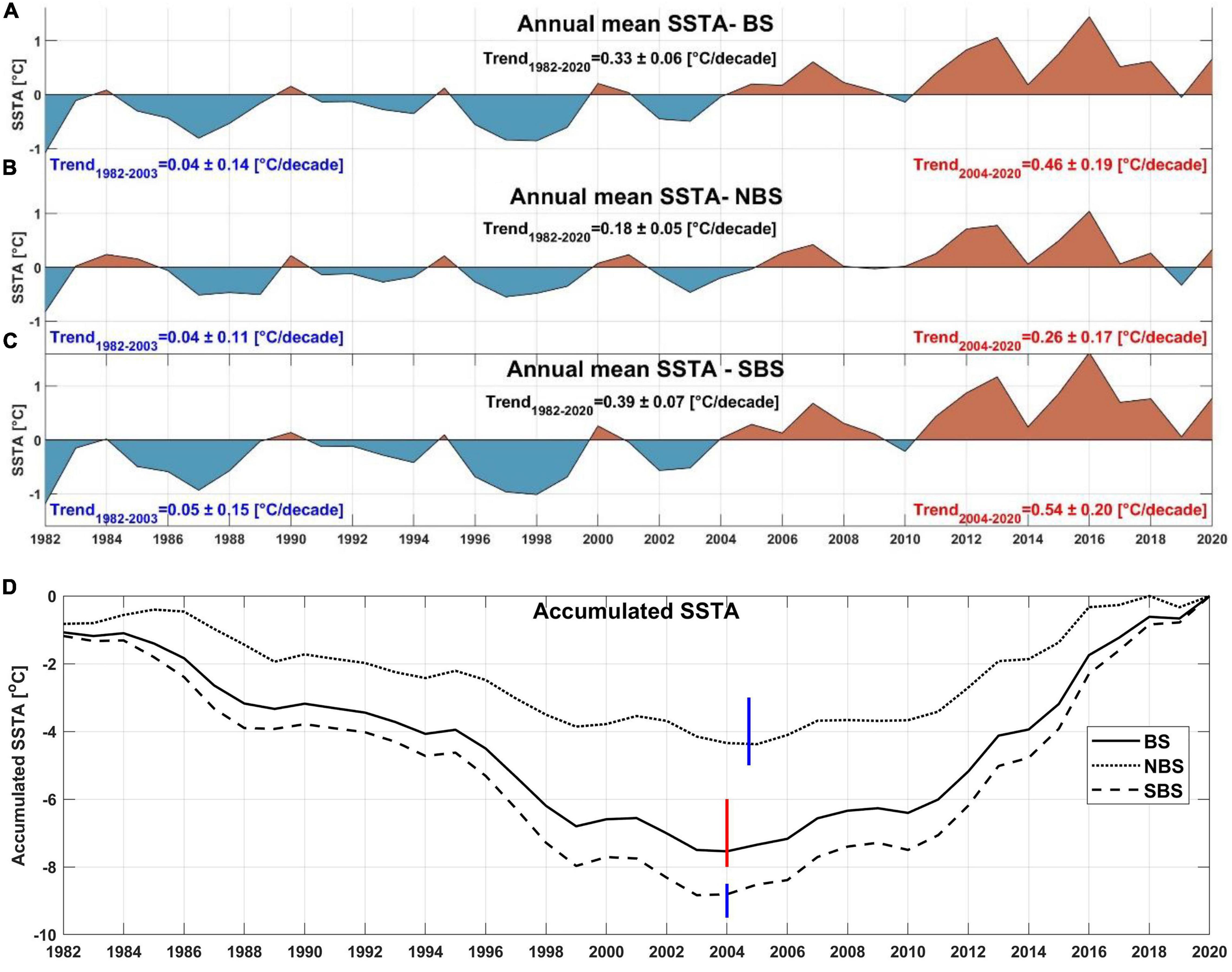
Figure 2. The temporal evolution of regionally averaged annual mean SST anomalies over (A) the entire (BS), (B) northern (NBS), and (C) southern (SBS) Barents Sea from 1982 to 2020 together with (D) long-term variation of cumulative anomalies over the same domains (see Figure 1). The vertical blue/red dashed lines represent the corresponding climate-shift year, which occurred in 2004 and 2005 over SBS and NBS, respectively. Note that the linear trend value (°C/decade) for each region for the various time periods is also provided.
Figures 2A–C depicts the temporal evolution of regional averaged annual mean SST anomalies in the BS, the NBS and the SBS from 1982 to 2020. The highest SSTA levels were recorded in 2016, with an average value of 1.0 and 1.6°C above the climatological (1982–2020) mean for the NBS and SBS, respectively. The most negative anomalies occurred in 1982. According to observations, SST over the SBS shifted from a period with episodic negative anomalies and a non-significant trend (1892–2003) to an amplified warming period since 2004 accompanied with a significant warming trend (Figure 2), though this shift seems to have occurred in 2005 for the NBS. From the annual accumulated SSTA time series over the BS (Figure 2D), there was a decreasing tendency (i.e., prevalence of negative anomalies) in the pre-2004 period and an increasing tendency (i.e., prevalence of positive anomalies) in the post-2004 period. These changing tendencies signify a climatic shift in 2004, and we found a significant temporal shift (Figure 2) and a significant spatial increase in the mean (Figures 3A–C) and trend (Figures 3H,I) of SST in recent decades (2004–2020). The regional climatological mean of SST over the entire Barents Sea for post-2004 was about 0.7°C higher than that for pre-2004 (Figures 3A–C). Figures 3D–F shows the spatial pattern in the standard deviations of the detrended SSTA throughout different time periods (the whole period, pre- and post-2004). These standard deviation values enable us to evaluate the total SST variability that is not explained by the seasonal cycle and linear trends. In general, the highest standard deviations (values are greater than 1°C) are observed over the different periods in the southeast Barents Sea and near the Svalbard Archipelago, as well as over the Polar Front, which closely follows the 220-m isobath (Barton et al., 2018). The region of the AW inflow has the lowest standard deviations (0.4–0.8°C). It should be noted that the maximum of the SST variations in the second period (2004–2020) also includes the eastern Barents Sea, the Storfjorden through and Storfjorden, and the western and northern shelf areas around Svalbard (Figures 3E,F). The increased variability could be the result of more AW at the sea surface when sea ice has retreaded along the AW pathways (Jakowczyk and Stramska, 2014; Lien et al., 2017) and intrusion of Atlantic Water on the Spitsbergen continental shelf (Nilsen et al., 2016).
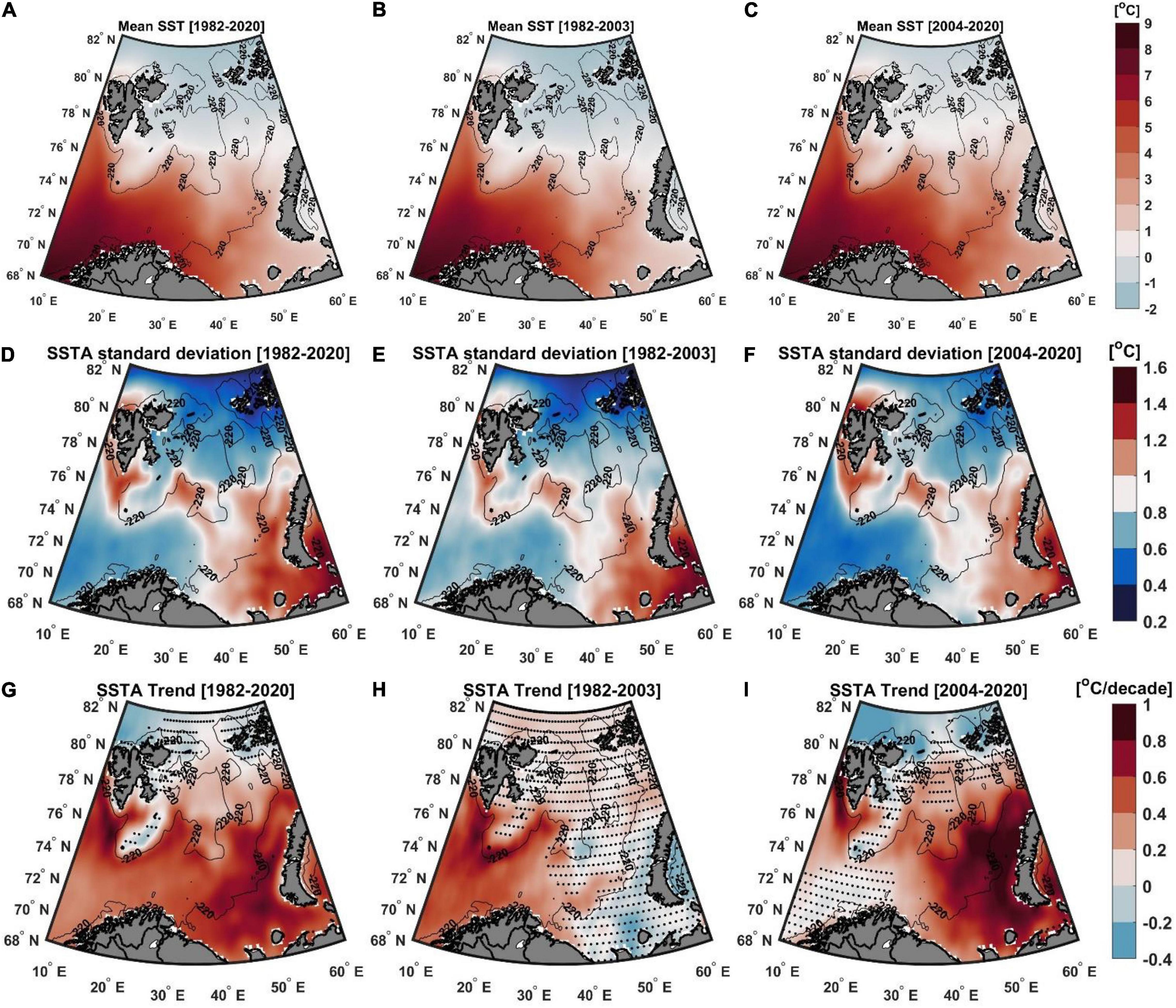
Figure 3. Spatial distribution of climatological mean SST (top panel row), standard deviation of the detrended SSTA (middle panel row), and SSTA trends (bottom panel row) for the periods: 1982–2020 (A,D,G), 1982–2003 (B,E,H), and 2004–2020 (C,F,I). Stippled regions indicate trends that are not statistically significant at the 95% confidence level. The black contour line represents the isobath of 220 m.
Positive statistically significant (p < 0.05) SSTA trends are observed over the entire Barents Sea from 1982 to 2020 (Figure 3G), except for Spitsbergen Bank and the northern part of the Barent Sea (mainly in the region north of 80°N), which exhibits a non-significant trend (p > 0.05). The spatial average SSTA trend was about 0.17 ± 0.05°C/decade and 0.41 ± 0.06°C/decade for NBS and SBS, respectively. The linear trend over the Barents Sea is not uniform, as shown in Figures 3G–I. Over the whole region for the pre-2004 period (Figure 3H), the SST trends were very low and not statistically significant, except in the southwestern region where warm Atlantic Water flows in Ingvaldsen et al. (2004) and Skagseth (2008). However, amplified warming trends were observed for the post-2004 period, except in the northwestern region where cold Arctic Water circulates (Lind et al., 2018). The overall spatially averaged warming trend was about 0.25 ± 0.18°C/decade and 0.58 ± 0.21°C/decade for NBS and SBS, respectively. Moreover, the SST trend exhibits high spatial variability over the Barents Sea, ranging from a minimum value of 0.00°C/decade (note that the negative trends are not statistically significant at 95% significant level) to a maximum of 1.00°C/decade (Figure 3I), accounting for a total increase of SST between 0.0 and 1.7°C over the Barents Sea since 2004. The highest SST trend is observed over the eastern part of the Barents Sea and south of Svalbard (the Storfjorden Trough), while a non-significant trend was found over the northern and southwestern Barents Sea. The high SST trends in the eastern Barents Sea are driven by an increase in warm AW inflow in the Kola Section (Barton et al., 2018) and reduced ocean heat loss over this region due to anomalous southerly winds (Skagseth et al., 2020).
The spatial distributions of the average annual mean MHW characteristics over the study period (1982–2020) are depicted in Figure 4. The Barents Sea exhibits a high spatial variability in all MHW characteristics. The MHW frequency varied from about 1.2 to 2.6 annual events, with higher frequencies (>2 events) over the northern Barents Sea and lower frequencies in the southeast region of the Barents Sea (Figure 4A). The total number of MHW days also varied significantly (Figure 4B), ranging from 20 days in open water regions (south of the climatological mean of April sea-ice edge, the solid white line in Figure 4B) to 32 days over the seasonal ice zone (north and southeast in the Barents Sea). Because of the thin sea ice thickness in the seasonal ice zone, shortwave and longwave fluxes from the atmosphere can pass through the ice and heat seawater when the atmosphere is warmer than the seawater, increasing the possibility of MHWs in this region (Hu et al., 2020). According to Toole et al. (2010), strong density stratification at the bottom of the surface mixed layer can inhibit surface layer deepening and hence limit vertical mixing. The presence of fresher, lighter surface waters in the northern Barents Sea ensures high stratification and limited upward fluxes from the warmer deeper layer (Lind et al., 2018). Long MHW duration of up to 24 days is observed in the southeast Barents Sea (Figure 4C), a region dominated by the inflow of warm Atlantic Water, while most of the study region shows an average of 10–16 days. The MHW mean intensities exhibit a dipole spatial pattern (Figure 4D), with the highest intensities of up to 2.4°C in the central and southeastern Barents Sea, which is affected by the positioning of the Polar Front separating warm Atlantic Water in the south from cold Arctic Water in the north while closely following the 220-m isobath (Barton et al., 2018), and lower values of 0.6–1.6°C in the northern Barents Sea and in the open water area in the southwestern Barents Sea. The higher MHW mean intensities over the Polar Front could be attributed to the high variability of SST in this region (Figures 3D–F). The spatial pattern of the maximum and cumulative MHW intensities is the same as that of the mean intensities and hence, we will not explore them further here. In general, MHWs are characterized by high frequency, short duration, and low intensity in NBS, and low frequency, long duration, and high intensity in the SBS. These different MHW characteristics can be linked to a reduced sea ice cover in winter (Onarheim et al., 2015) and a weakened vertical stratification (Lind et al., 2018) in the NBS that makes it easier to mix up more AW and responsible of MHW with a higher frequency, a shorter duration, and lower intensity as compared to the SBS MHWs, which could be driven by a more persistent wind forced volume transport of AW with a strong surface signal (Ingvaldsen et al., 2004) and southerly off-shore wind form land with warm air over the SBS.
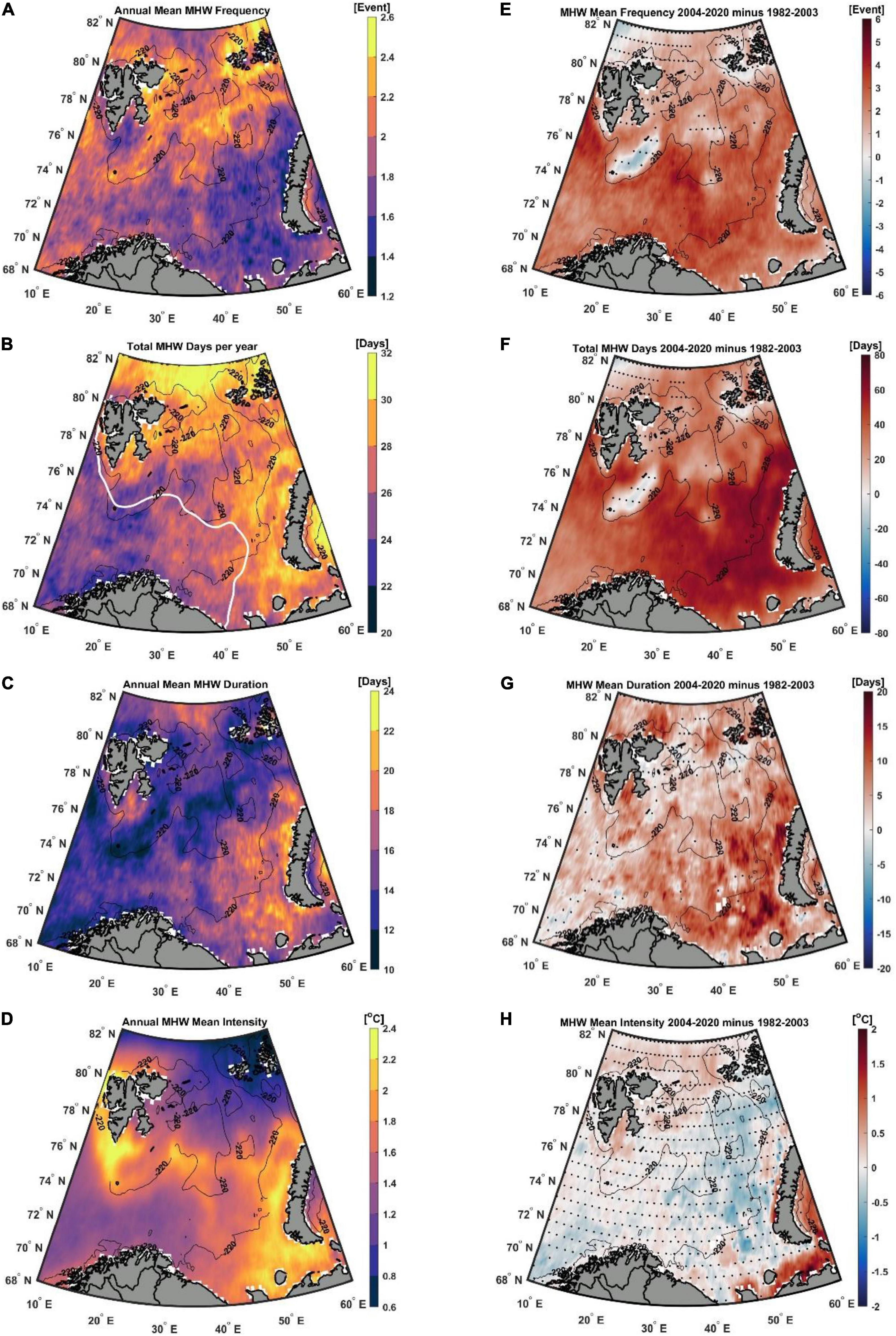
Figure 4. The spatial distribution of the annual mean of the main MHW characteristics in the Barents Sea from 1982 to 2020, (A) MHW frequency (events); (B) MHW Days (days) the white contour line represents the climatological mean of April sea-ice edge (15% SIC); (C) MHW duration (days); (D) MHW mean intensity (°C); and difference between the post-2004 and pre-2004 (E) MHW frequency (events); (F) MHW Days (days); (G) MHW duration (days); (°C); (H) MHW mean intensity (°C). In (E–H), stippled regions indicate the change is non-significantly different from zero at the 95% confidence interval (p > 0.05), based on the standard two-sample Student t-test. The black contour lines indicate the isobath of 220 m.
A climate shift in 2004 has been identified through the accumulated SSTA time series (Figure 2D), and the changes in MHW characteristics from pre- to post-2004 periods are therefore calculated. The annual mean MHW frequency increased by 62% between these periods and the highest rise occurred in the southern Barents Sea (an increase of 4–6 annual events). More moderate increases (1–3 annual events) were recorded in the northern Barents Sea (Figure 4E), while non-significant changes (p > 0.05) were observed over the Spitsbergen Bank, north of 80°N, and in a portion of Storbanken. Annual mean MHW days increased by 73% over the entire Barents Sea between the pre-and post-2004 periods and showed the same spatial pattern as frequency (Figure 4F). The annual mean MHW duration increased by 31% between the two periods, with a significant increase over most of the Barents Sea with a maximum value of up to 20 days in the southeastern Barents Sea (Figure 4G). There is no statistically significant difference (p > 0.05) in annual MHW mean intensity between the two periods (Figure 4H), except over the Kara Sea and along the Eurasian coast; however, there is a mean MHW intensity reduction in the SBS and along the AW pathway, with a slight increase in the northwestern BS.
The spatial distributions of long-term trends (1982–2020) in annual mean MHW characteristics are shown in Figure 5. MHW frequency and days reveal a statistically significant (p < 0.05) positive trend over the whole Barents Sea, except for the Spitsbergen Bank and the northern part of the Barent Sea (mainly in the region north of 80°N). The regional patterns of trends in MHW frequency and days are consistent with the observed trends in SST warming and cooling over the same period (Figure 3A), indicating that SST trends most likely have a substantial impact on MHW genesis over the whole region. The highest MHW frequency decadal trends (up to 2 events/decade) are found over the southern Barents Sea and in the Storfjorden Trough (Figure 5A). The trends in total number of MHW days varied from 10 to 35 days/decade, except for the area north of 80°N and the Spitsbergen Bank, which indicate a non-significant trend, while the maximum values of more than 30 days/decade are observed over the southeastern Barents Sea (Figure 5B).
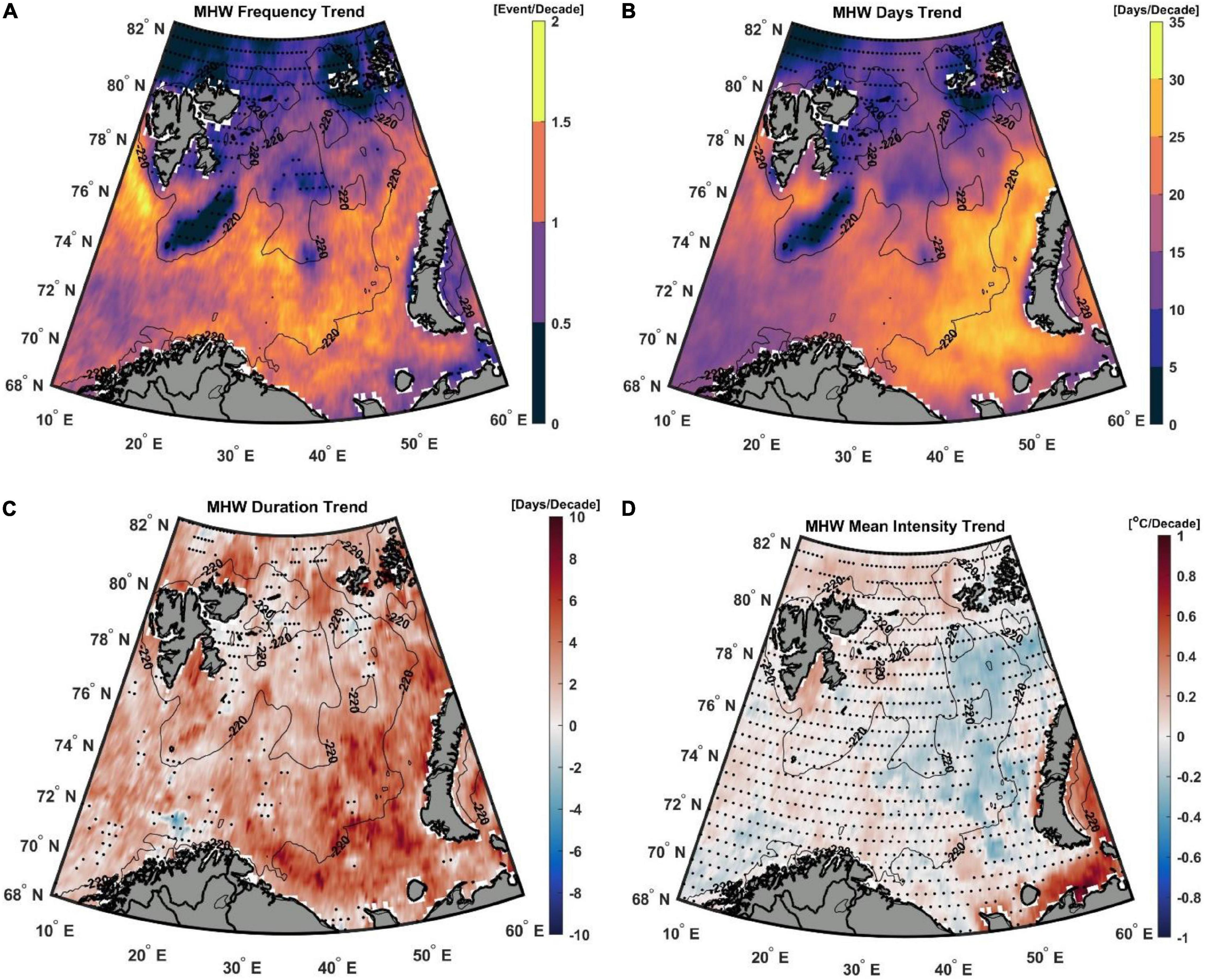
Figure 5. Decadal trends in marine heatwave characteristics in the Barents Sea over the period 1982–2020 with (A) MHW frequency (events/decade), (B) MHW days (days/decade), (C) MHW duration (days/decade), and (D) MHW mean intensity (°C/decade). Stippled regions indicate that the trend is statistically non-significant at the 95% confidence interval (p > 0.05).
The maximum and most significant trends in MHW duration (Figure 5C) are detected in the SBS and along the AW pathway toward the northeast, in the same regions that have experienced higher SST increase throughout the warming period 2004–2020 (Figure 3D). Trends with longer MHW duration (up to 10 days/decade) are observed in the southeastern Barents Sea (Figure 5C). Non-significant trends in MHW mean intensities are seen over the whole Barents Sea (Figure 5D), with only two regions (the Kara Sea and along the Eurasian coast) showing a significant trend with values up to 1°C/decade. In general, the SBS contains the highest significant trends in the MHW characteristics. However, this pattern has extended further northward during the recent decades, due to the strong northward and eastward SIC retreat (Herbaut et al., 2015) and SST rise that have been documented since 2004 (Figure 3I).
In this section, we look at how the regional average (BS, SBS, and NBS) of the annual mean MHW characteristics (frequency, days, duration, and cumulative intensity) changed from 1982 to 2020 in relation to the annual mean sea surface temperature (Figure 6). In total, 72 MHWs were recorded in the whole Barents Sea over the 39-years study period with a total of 1,068 MHW days. Since January 2004, a total of 876 MHW days has occurred, indicating an increasing trend in days with MHW duration and intensity, and 2016 stands out with a record of 200 MHW days. Moreover, the highest annual MHW frequencies were detected in 2016 (7 events), 2012 (5 events), 2013 (5 events), and 2015 (5 events). These findings are consistent with the SSTA in Figure 2A. The highest annual MHW cumulative intensity and duration are observed in 2016, 2013, and 2020. In 2016, the annual mean MHW duration was about 32 days with a cumulative intensity of approximately 75°C days. The NBS has a higher frequency and a total number of MHW days than SBS, except for the last 5 years (Figures 6A,B) where the mean intensities are higher in the SBS (Figure 6D).
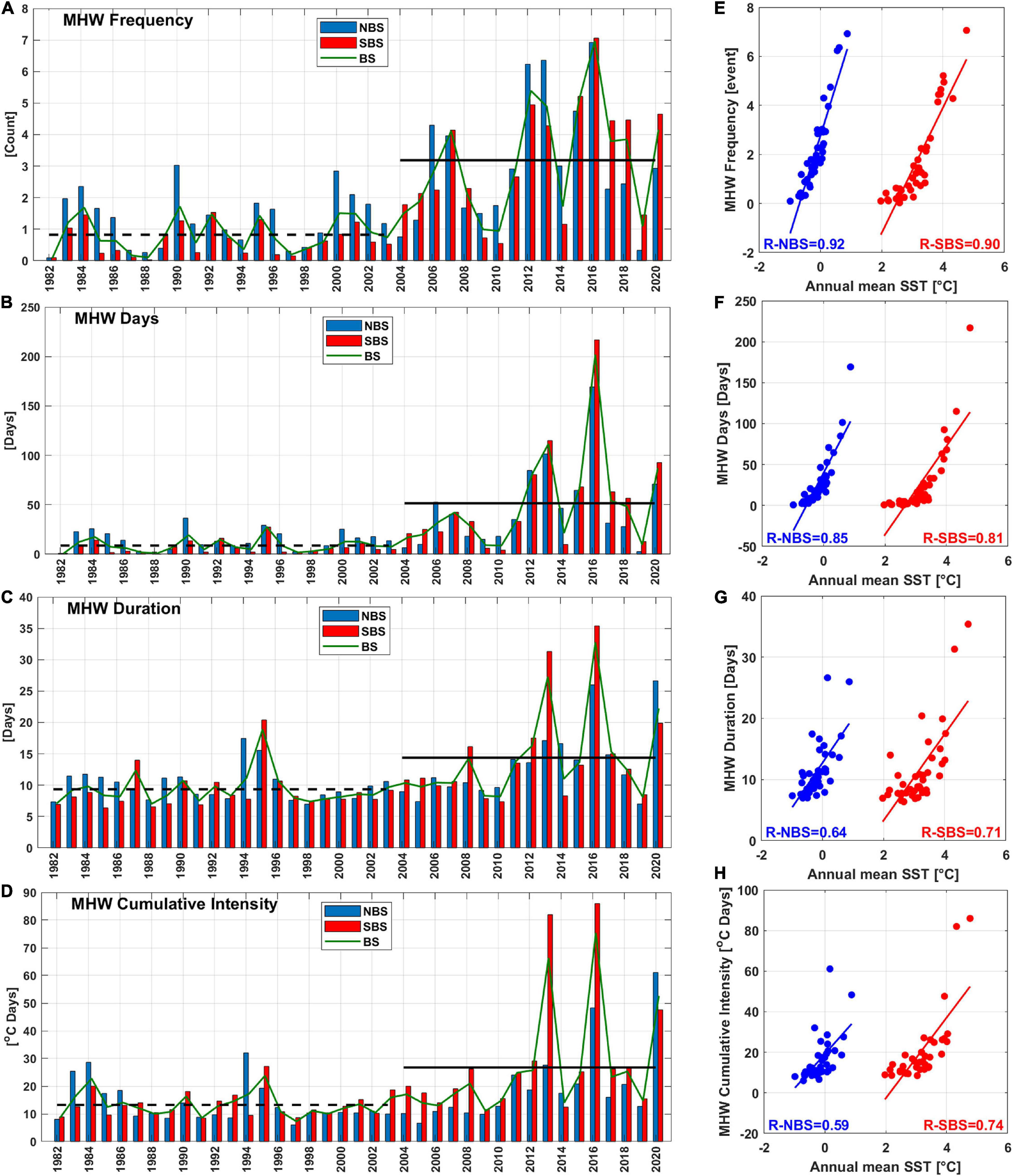
Figure 6. Regionally averaged annual means of the MHW (A) frequency (events/year), (B) days (days/year), (C) duration (days/year), and (D) cumulative intensity (°C days/year). The blue and red bars represent the northern and southern Barents Sea (NSB and SBS), respectively. The green lines represent the whole Barents Sea (BS). The black dashed and solid lines represent the mean value for the whole BS over the pre- and post-2004 period, respectively. The right panels show the scatter plots of annual mean SST versus annual mean MHW (E) frequency, (F) days, (G) duration, and (H) cumulative intensity over NBS (blue) and SBS (red) from 1982 to 2020, with the blue and red lines representing the best-fit linear curve.
The MHW characteristics (frequency, days, duration, and cumulative intensity) over the Barents Sea show a clear ascending trend from 1982 to 2020 (Figures 6A–D). Annual mean MHW frequency tripled from the pre- to post-2004 periods, from ∼ 1 event/year during 1982–2003 to ∼3 events/year during 2004–2020. There is also a general increase in MHW duration from about 10 days to 14 days (1.4 times increase) and cumulative intensity from 13.6°C days to 24.8°C days (1.8 times increase) between the pre- and post-2004 periods. Hence, we can conclude that MHWs have become longer, more frequent, and more intense during the warming period than before 2004.
Furthermore, the frequency and duration of MHWs in the whole Barents Sea increased significantly (p < 0.05) over the entire study period with a trend of about 1.0 ± 0.4 events/decade and 2.4 ± 1.3 days/decade, respectively. For comparison purpose, we evaluated the trend in annual MHW frequency in the Barents Sea from 1982 to 2016, and found that this trend (1.12 events/decade) is more than twice as high as the global averaged trend (0.45 events/decade) for the same period (Oliver et al., 2018). Over the entire study period, the regional annual mean SST and annual mean MHW frequency, duration, and cumulative intensity over NBS and SBS are highly correlated at 95% confidence interval (p < 0.05) (Figures 6E–H). The strongest relationship was found between SST and MHW frequency, with correlation coefficients of 0.92 and 0.90 for NBS and SBS, respectively. It should be noted that the Arctic and particularly the Barents Sea is a hotspot in the global warming trend (Lind et al., 2018; Schlichtholz, 2019), resulting in an increase in MHW events.
In this section, we will look at the role of the two major climate modes, NAO and EAP, on the occurrences of MHWs in the Barents Sea. Figure 7 depicts the correlation between the yearly count of MHWs frequency (occurrences) and these two climate modes. At the annual scale, the EAP shows a significant positive correlation with MHW frequency over most of the Barents Sea, with the highest correlation in the southeast of the Barents Sea. Furthermore, the EAP has a significant correlation with all MHW characteristics during summer (Table 1), as most of the strong positive phase of EAP is observed in the summer, whereas this correlation was non-significant in winter except for MHW frequency (R = 0.38). The highest correlations between NAO and MHWs are observed with 7-month lags in MHW response to NAO. However, at both the annual and seasonal scales, these correlations were not statistically significant (Figure 7 and Table 1). These findings are consistent with (Chafik et al., 2017), who studied the impact of NAO and EAP on northern European sea level and have found that the sea level response to EAP is significant over the entire Barents Sea, whereas the NAO showed a non-significant relationship except along the coastal regions.
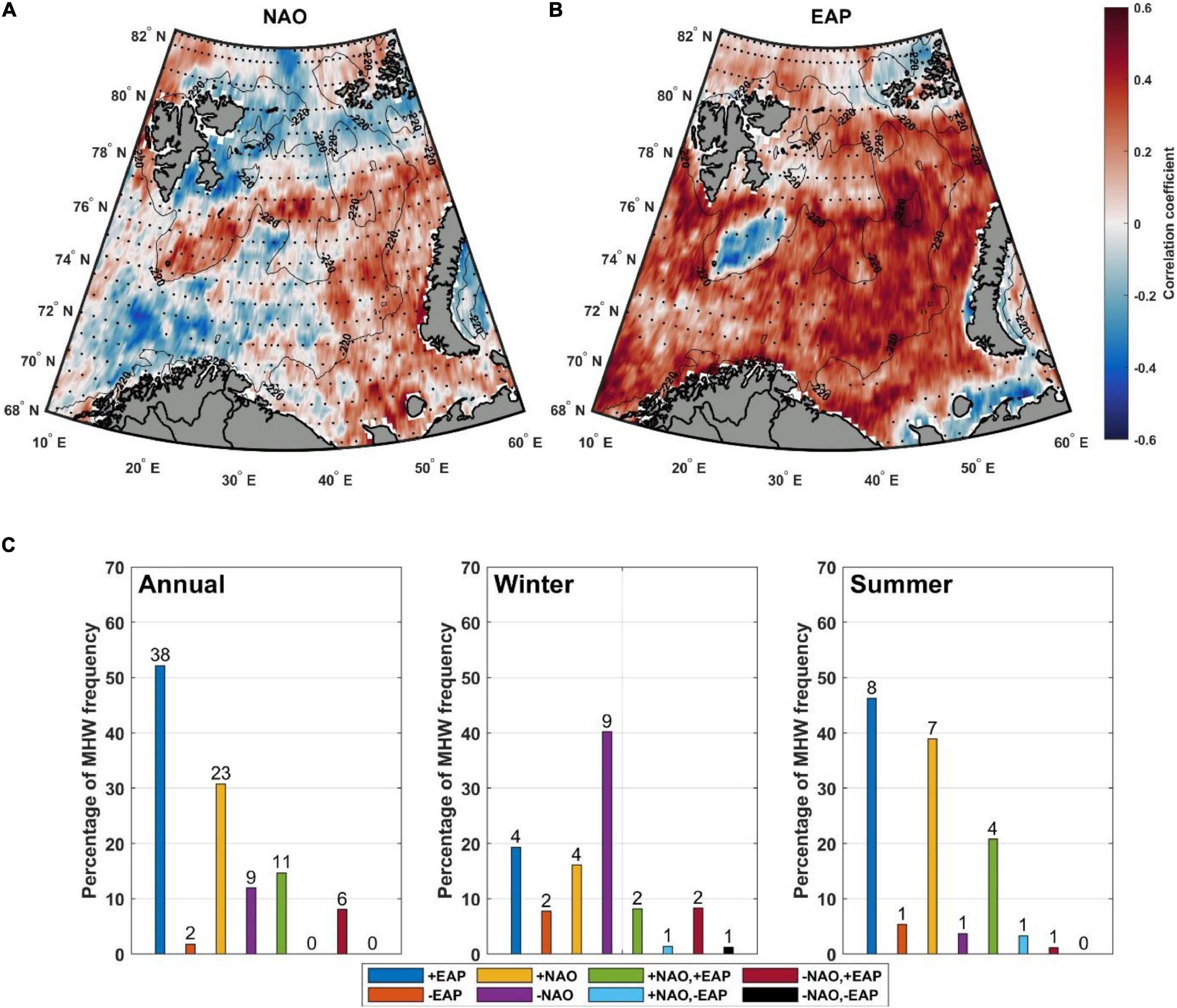
Figure 7. Correlation coefficients between MHW frequency and two major climate modes: (A) NAO, (B) EAP. Stippled regions indicate that the correlations are statistically non-significant at the 95% confidence level (p > 0.05). (C) The percentage of MHW occurrences that coincide with climate modes for the entire year, winter, and summer. The numbers above the bars represent the total number of MHW.
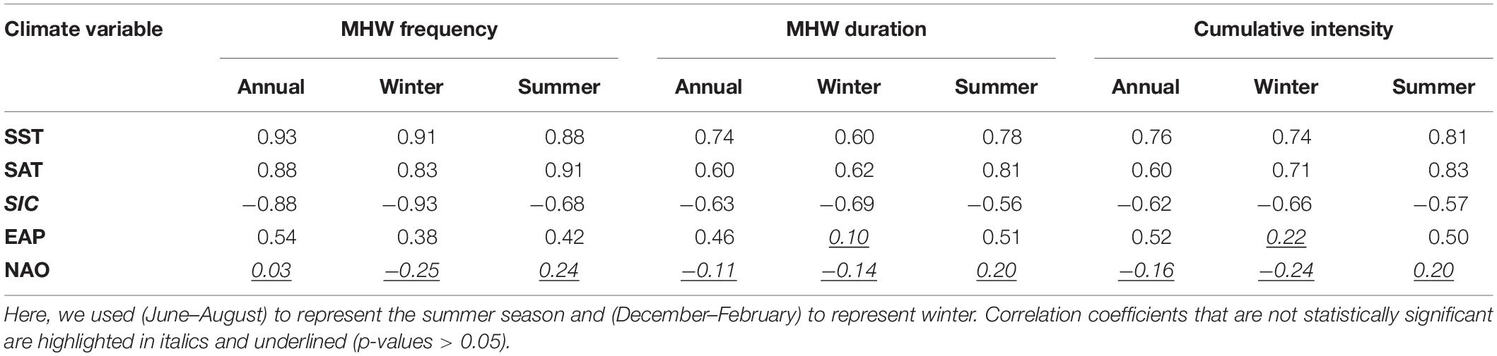
Table 1. Correlation coefficients (R) between MHW characteristics (frequency, duration, and cumulative intensity) and climate modes (EAP and NAO) and variables (SST, SAT, and SIC).
A composite analysis of MHW occurrences and climate modes or overlapping modes (Figure 7C) shows that more than half of the MHWs occurred during the positive phase of EAP, which was associated with above-average surface temperatures in Europe throughout the year5. Though the NAO is not correlated with all MHW characteristics, approximately 30% of the MHWs occurred during the NAO’s positive phase, as the composite analysis only considers the strong positive phases (exceeds 1 standard deviation). When both the NAO and the EAP are in the positive phase, about 15% of the MHWs occur, while there are no MHWs when both are in the negative phase. Noticeably, about 30% of the MHWs occur when no active climate modes are present (i.e., there are no positive or negative phases). The coexistence rate of MHWs with positive EAP or NAO modes is higher in summer than in winter. The strong correlation and higher coexistence of MHWs with the EAP mode, indicates that the EAP mode plays an important role in modulating MHWs in the Barents Sea.
The correlation coefficients between MHW characteristics (frequency, duration, and cumulative intensity) and essential climate variables, SST, SAT, and SIC for the entire Barents Sea are summarized in Table 1. At annual and seasonal scales, SST and SAT exhibit a highly significant positive relationship with all MHW characteristics, indicating that besides the SST rise, atmospheric warming most likely plays an important role in the formation of MHWs in the Barents Sea. Seasonal behavior is also shown to have a strong positive correlation in the summers and winters, with higher values in the summers. The winter and summer differences for the SST and SAT correlation with the MHW frequency could be explained by more AW water at the surface in some areas during winter increasing the SST and MHW, while the large summer correlation coefficient between SAT and MHW frequency is linked to more southerly winds with warmer air masses over the Barents Sea. The SIC has a strong negative correlation with MHW frequency (R = −0.88), duration (R = −0.63), and cumulative intensity (R = −0.62). This indicates that low SIC years have more MHW events, longer MHW durations, and higher MHW intensities. The relationship between SIC and MHW characteristics is stronger in winter than in summer since the sea ice cover is largest in winter and makes the feedback stronger in years with anomalous low sea ice cover.
In this section, we discuss all the MHW events that were detected in 2016 over NBS and SBS as well as the atmospheric conditions during the “strong” MHW event occurring in SBS between 28 June and 29 August 2016. Moreover, this MHW extended northwards into NBS during the same period. Seven MHWs were detected in NBS and SBS in 2016 (Figure 8). According to the Hobday et al. (2018) classification of MHWs, the intensity of these MHWs ranged from moderate (i.e., the SSTA > the 90th percentile threshold anomaly) to strong (i.e., SSTA is greater than twice the 90th percentile threshold anomaly) and the duration ranged from 5 to 92 days. The longest MHW event was observed in SBS during the autumn season, lasting for 92 days from 4 September to 5 December, and then extending into NBS for 69 days from 29 September to 6 December. During this event, the mean MHW intensities were approximately 1.55 and 1.85°C with maximum intensities of approximately 2.15 and 2.29°C for NBS and SBS, respectively. The two shortest MHWs were observed during the winter season; in NBS, both are detected in December, while in SBS, one is detected in December and the other in the late of March.
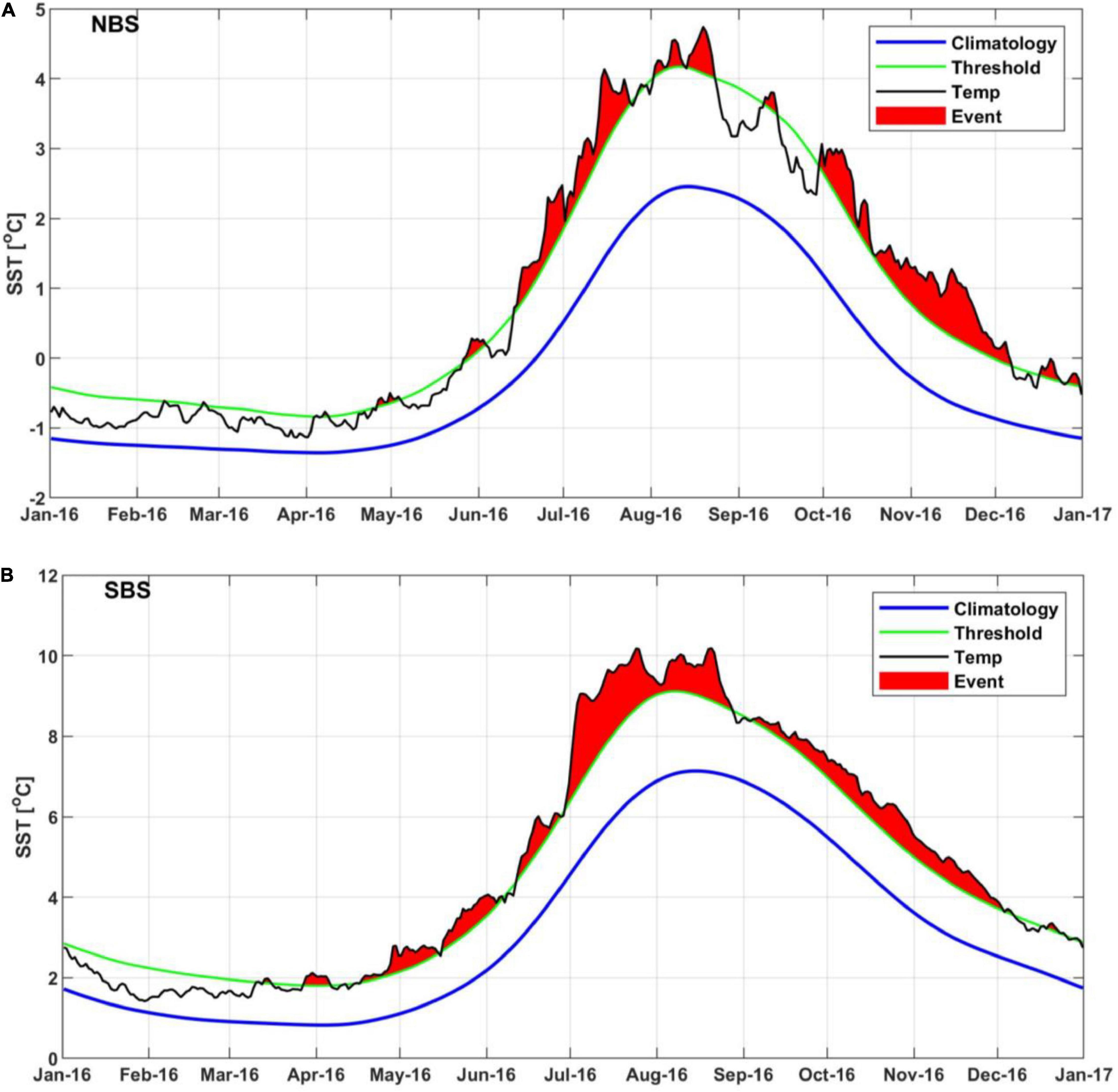
Figure 8. Evolution of the daily SST time series within (A) the northern Barents Sea (NBS), and (B) the southern Barents Sea (SBS) from January to December 2016 (black lines). The blue line represents the daily climatology over a 39-years period (1982–2020). The green line represents the seasonally varying 90th percentile threshold. Red shaded regions indicate the period associated with the identified MHWs. The y-axes for the two plots are different to increase visibility, as the SST varies greatly from NBS to SBS.
The most intense MHW event occurred in SBS from 28 June to 29 August 2016, with a mean and maximum intensity of 2.96 and 4.13°C, respectively, and a duration of 63 days. This event is classified as a strong MHW event and extended also into the NBS. It split into two events, one which continued from spring and the other which occurred in August. Figure 9A depicts the average SSTA during this event, where the average SSTA over the entire Barents Sea was about 2.5°C and negative SSTA values were only found north of 80°N. The average SSTA in NBS and SBS was about 1.8 and 2.9°C, respectively. Previous biological studies by Eriksen et al. (2020), which focused on the spatial distributions of fish abundance in the Barents Sea in relation to environmental conditions in 2016, have found that some marine species reacted to the warm water condition during this strong MHW event by shifting their geographic distribution. Compared to the previous 5 years (2011–2015), the densest cod and herring aggregations shifted eastward, while capelin aggregations shifted northward. Species, such as capelin, haddock, herring, and long rough dab were more abundant than the long-term average (1980–2016), whereas polar cod abundance was significantly lower and had nearly disappeared in the core area of the southeastern Barents Sea where the most intense MHWs are found.
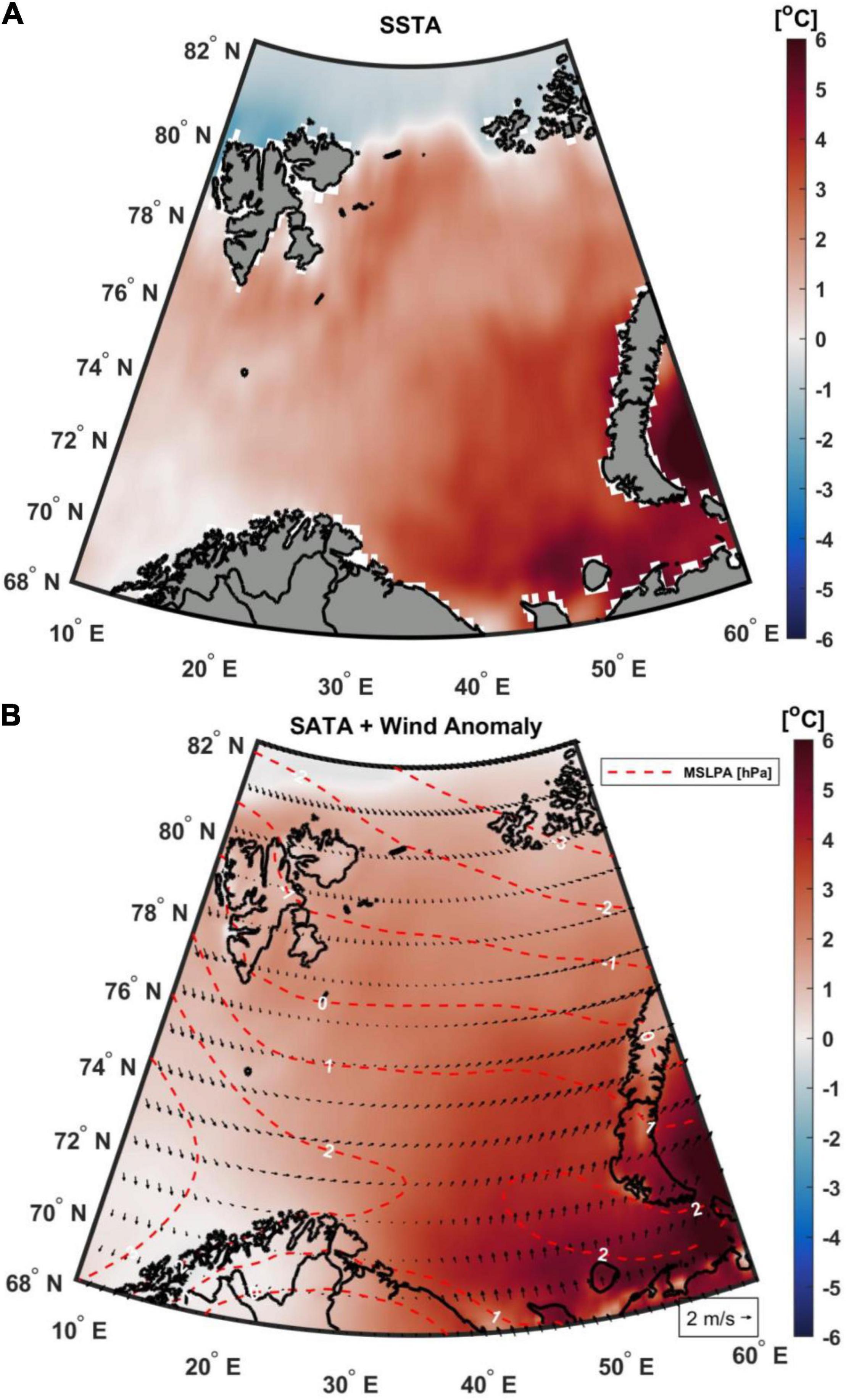
Figure 9. (A) Spatial distribution of mean SST anomaly (SSTA) in the Barents Sea during the most intense (“strong”) MHW event (28 June to 29 August 2016), (B) Corresponding anomalies in 2 m air temperature (SATA, shaded), mean sea level pressure (MSLPA, dashed contours red line, units: hPa), and wind velocity anomalies (black arrows denote magnitude and direction of wind anomaly, scale arrow at bottom right, units: m/sec).
The atmospheric states during the strong MHW event (from June 28 to August 29, 2016) revealed warm atmospheric temperature anomalies across the entire Barents Sea, with the highest values observed in the southeastern Barents Sea (Figure 9B), which coincides with the same region of the most intense MHW event. During this event, higher atmospheric pressure anomalies (up to + 2 hPa) are observed over the southeast of the Barents Sea. The persistence of a high-pressure system over the ocean reduces cloud cover, increases solar radiation, and reduces surface wind speed, resulting in hot and dry weather that contributes to SST warming (Holbrook et al., 2020). The wind anomaly patterns during this period were southerly anomalies over the southeast of the Barents Sea and weak northwesterly anomalies over the NBS, resulting in transport of heat and humidity from the south to the northern Barents Sea and causing a strong summer MHW across the entire Barents Sea. This combination of unusually southerly wind (negative anomalies) and higher atmospheric pressure over the southeast of the Barents Sea most likely resulted in an intense positive loop of surface heating and stratification that was unable to break due to insufficient wind stress to mix up colder water from below. Moreover, the strongest positive phase of EAP was observed during this event (Figure 10), which is commonly associated with southerly wind anomalies (Figure 9) and above-average surface temperatures over northwest Europe. In conclusion, the main cause of this strong MHW event was most likely atmospheric overheating, which was accompanied by a southerly wind and abnormally high pressure. Further dataset and analysis are required to investigate all the possible drivers of MHWs in the Barents Sea, including heat advection by the ocean current.
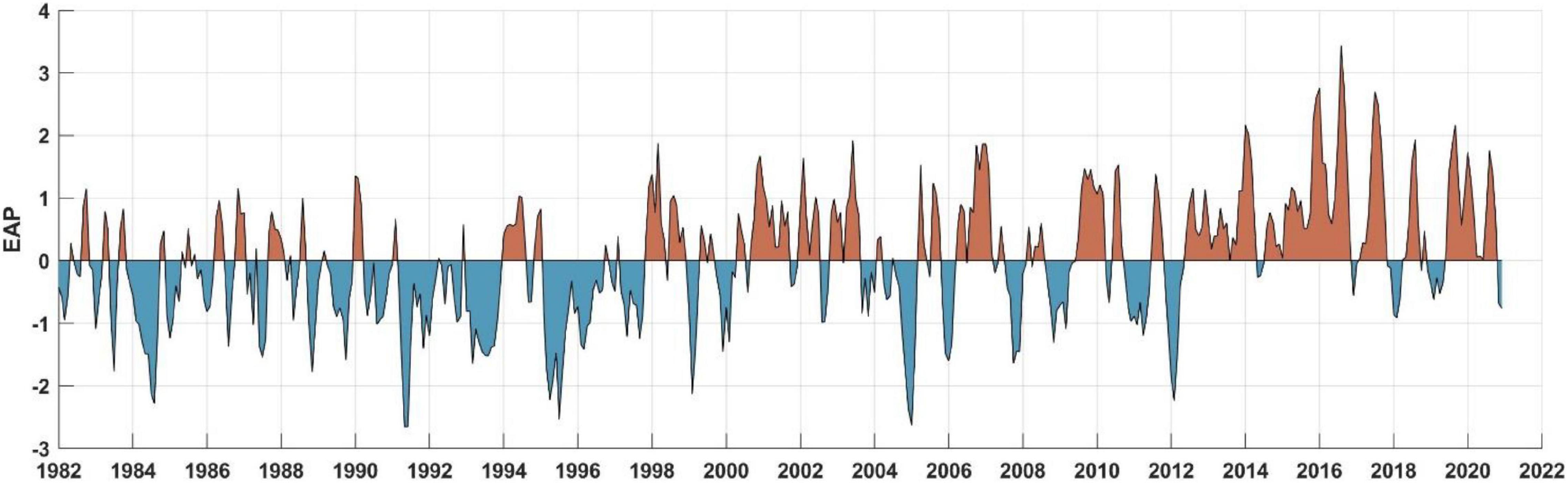
Figure 10. Standardized 3-months running mean values of the Eastern Atlantic Pattern (EAP) index from 1982 to 2020. Note that the strongest positive phase of EAP coincided with the most intense MHW event throughout the summer of 2016.
The Barents Sea is considered a major climate change hotspot. Based on high-resolution SST data, this paper provides a comprehensive analysis of the change in SST and the spatiotemporal evolution of MHW characteristics in the Barents Sea from 1982 to 2020. One of the study’s key findings is that the Barents Sea experienced a significant warming shift in 2004, which is consistent with Lind et al. (2018) that found a sharp increase in ocean temperature and salinity from the mid-2000s, and with Skagseth et al. (2020), demonstrating a warming of near-bottom temperatures starting from 2004. The spatial average of the SST warming rate from 2004 to 2020 was about 0.25 ± 0.18°C/decade and 0.58 ± 0.21°C/decade for the northern and southern Barents Sea, respectively. Secondly, the Barents Sea is most likely a high-risk region for the impact of MHWs, as the frequency and duration of MHWs have increased significantly between 1982 and 2020. The average MHW frequency trend was about 1.0 ± 0.4 events/decade, which is more than double the global averaged trend of 0.45 events/decade (Oliver et al., 2018). The average trend of MHW duration was about 2.4 ± 1.3 days/decade. The most intense MHW event was observed in the southern Barents Sea and lasted 63 days from 28 June to 29 August 2016, with mean and maximum intensities of 2.96 and 4.13°C, respectively. MHWs are characterized by high frequency, short duration, and low intensity in the northern Barent Sea, and low frequency, long duration, and high intensity in the southern Barents Sea. Our analyses suggested that the growing trends in MHWs in the Barents Sea were most likely forced by warm surface air and decreasing sea ice, which was facilitated by SST-ice feedback and mostly driven by increased oceanic heat advection and convection (getting the warm water up to the surface) (Årthun et al., 2012; Onarheim et al., 2015; Lien et al., 2017). In winter, surface air temperatures are also driven by oceanic heat advection/convection when the sea ice cover is gone. Future research is required to investigate all the potential causes of MHWs in the Barents Sea, including heat advection by ocean currents, as proposed by multiple related studies (Oliver et al., 2017; Huang et al., 2021b).
Excessive SST warming rates and MHWs in the Barents Sea are expected to have far-reaching environmental and societal consequences in this region. More research is needed to predict future MHWs in the Barents Sea using model experiments and to study their effects on marine life. To be able to implement appropriate early warning procedures related to thermal stress on various marine ecosystems, as well as to find appropriate regional climate policies to deal with climatic change issues. Particularly, the Barents Sea has diverse marine ecosystems and fishing grounds.
The original contributions presented in the study are included in the article, further inquiries can be directed to the corresponding author.
BM, FN, and RS: conceptualization, methodology, software, validation of results, formal analysis, investigation, resources, data curation, writing, review, editing, and visualization. BM: writing – original draft preparation. FN and RS: supervision, project administration, and funding acquisition. All authors have read and agreed to the published version of the manuscript.
This work was fully funded by the Research Council of Norway through the Nansen Legacy Project (RCN # 276730).
The authors declare that the research was conducted in the absence of any commercial or financial relationships that could be construed as a potential conflict of interest.
All claims expressed in this article are solely those of the authors and do not necessarily represent those of their affiliated organizations, or those of the publisher, the editors and the reviewers. Any product that may be evaluated in this article, or claim that may be made by its manufacturer, is not guaranteed or endorsed by the publisher.
We would like to thank the organizations that provided the data used in this work, including the National Oceanic and Atmospheric Administration (NOAA) and the European Centre for Medium-Range Weather Forecasts (ECMWF). We would also like to express their gratitude to the reviewers for their contributions to the development of this manuscript.
Arias-Ortiz, A., Serrano, O., Masqué, P., Lavery, P. S., Mueller, U., Kendrick, G. A., et al. (2018). A marine heatwave drives massive losses from the world’s largest seagrass carbon stocks. Nat. Clim. Chang. 8, 338–344. doi: 10.1038/s41558-018-0096-y
Årthun, M., Eldevik, T., Smedsrud, L. H., Skagseth, Ø., and Ingvaldsen, R. B. (2012). Quantifying the influence of atlantic heat on barents sea ice variability and retreat. J. Clim. 25, 4736–4743.
Asbjørnsen, H., Årthun, M., Skagseth, Ø., and Eldevik, T. (2020). Mechanisms underlying recent arctic atlantification. Geophys. Res. Lett. 47:e2020GL088036.
Banzon, V., Smith, T. M., Chin, T. M., Liu, C., and Hankins, W. (2016). A long-term record of blended satellite and in situ sea-surface temperature for climate monitoring, modeling and environmental studies. Earth Syst. Sci. Data 8, 165–176. doi: 10.5194/essd-8-165-2016
Banzon, V., Smith, T. M., Steele, M., Huang, B., and Zhang, H.-M. (2020). Improved estimation of proxy sea surface temperature in the arctic. J. Atmos. Ocean. Technol. 37, 341–349. doi: 10.1175/JTECH-D-19-0177.1
Barton, B. I., Lenn, Y. D., and Lique, C. (2018). Observed atlantification of the Barents Sea causes the Polar Front to limit the expansion of winter sea ice. J. Phys. Oceanogr. 48, 1849–1866. doi: 10.1175/JPO-D-18-0003.1
Benthuysen, J. A., Oliver, E. C. J., Feng, M., and Marshall, A. G. (2018). Extreme marine warming across tropical australia during austral summer 2015–2016. J. Geophys. Res. Oceans 123, 1301–1326. doi: 10.1002/2017JC013326
Bojinski, S., Verstraete, M., Peterson, T. C., Richter, C., Simmons, A., and Zemp, M. (2014). The concept of essential climate variables in support of climate research, applications, and policy. Bull. Am. Meteorol. Soc. 95, 1431–1443. doi: 10.1175/BAMS-D-13-00047.1
Bond, N. A., Cronin, M. F., Freeland, H., and Mantua, N. (2015). Causes and impacts of the 2014 warm anomaly in the NE Pacific. Geophys. Res. Lett. 42, 3414–3420. doi: 10.1002/2015GL063306
Chafik, L., Nilsen, J. E. Ø., and Dangendorf, S. (2017). Impact of north atlantic teleconnection patterns on northern european sea level. J. Mar. Sci. Eng. 5:43. doi: 10.3390/JMSE5030043
Chafik, L., Nilsson, J., Skagseth, Ø., and Lundberg, P. (2015). On the flow of Atlantic water and temperature anomalies in the Nordic Seas toward the Arctic Ocean. J. Geophys. Res. Oceans 120, 7897–7918. doi: 10.1002/2015JC011012
Chen, K., Gawarkiewicz, G., Kwon, Y.-O., and Zhang, W. G. (2015). The role of atmospheric forcing versus ocean advection during the extreme warming of the Northeast U.S. continental shelf in 2012. J. Geophys. Res. Ocean. 120, 4324–4339. doi: 10.1002/2014JC010547
Chen, K., Gawarkiewicz, G. G., Lentz, S. J., and Bane, J. M. (2014). Diagnosing the warming of the Northeastern U.S. Coastal Ocean in 2012: a linkage between the atmospheric jet stream variability and ocean response. J. Geophys. Res. Oceans 119, 218–227. doi: 10.1002/2013JC009393
Dalpadado, P., Arrigo, K. R., Hjøllo, S. S., Rey, F., and Ingvaldsen, R. B. (2014). Productivity in the barents sea-response to recent climate variability. PLoS One 9:95273. doi: 10.1371/journal.pone.0095273
Dalpadado, P., Ingvaldsen, R. B., Stige, L. C., Bogstad, B., Knutsen, T., Ottersen, G., et al. (2012). Climate effects on Barents Sea ecosystem dynamics. ICES J. Mar. Sci. 69, 1303–1316. doi: 10.1093/ICESJMS/FSS063
Di Lorenzo, E., and Mantua, N. (2016). Multi-year persistence of the 2014/15 North Pacific marine heatwave. Nat. Clim. Change 6, 1042–1047. doi: 10.1038/nclimate3082
Eriksen, E., Bagøien, E., Strand, E., Primicerio, R., Prokhorova, T., Trofimov, A., et al. (2020). The record-warm barents sea and 0-group fish response to abnormal conditions. Front. Mar. Sci. 7:338. doi: 10.3389/FMARS.2020.00338
Frölicher, T. L., Fischer, E. M., and Gruber, N. (2018). Marine heatwaves under global warming. Nature 560, 360–364. doi: 10.1038/s41586-018-0383-9
Frölicher, T. L., and Laufkötter, C. (2018). Emerging risks from marine heat waves. Nat. Commun. 9:650. doi: 10.1038/s41467-018-03163-6
Garrabou, J., Coma, R., Bensoussan, N., Bally, M., Chevaldonné, P., Cigliano, M., et al. (2009). Mass mortality in Northwestern Mediterranean rocky benthic communities: effects of the 2003 heat wave. Glob. Change Biol. 15, 1090–1103. doi: 10.1111/J.1365-2486.2008.01823.X
Hamed, K. H., and Ramachandra Rao, A. (1998). A modified Mann-Kendall trend test for autocorrelated data. J. Hydrol. 204, 182–196. doi: 10.1016/S0022-1694(97)00125-X
Herbaut, C., Houssais, M. N., Close, S., and Blaizot, A. C. (2015). Two wind-driven modes of winter sea ice variability in the Barents Sea. Deep Res. Part I Oceanogr. Res. Pap. 106, 97–115. doi: 10.1016/j.dsr.2015.10.005
Hersbach, H., Bell, B., Berrisford, P., Hirahara, S., Horányi, A., Muñoz-Sabater, J., et al. (2020). The ERA5 global reanalysis. Q. J. R. Meteorol. Soc. 146, 1999–2049. doi: 10.1002/qj.3803
Hobday, A. J., Alexander, L. V., Perkins, S. E., Smale, D. A., Straub, S. C., Oliver, E. C. J., et al. (2016). A hierarchical approach to defining marine heatwaves. Prog. Oceanogr. 141, 227–238. doi: 10.1016/j.pocean.2015.12.014
Hobday, A. J., Oliver, E. C. J., Gupta, A. S., Benthuysen, J. A., Burrows, M. T., Donat, M. G., et al. (2018). Categorizing and naming marine heatwaves. Oceanography 31, 162–173. doi: 10.5670/oceanog.2018.205
Holbrook, N. J., Scannell, H. A., Sen Gupta, A., Benthuysen, J. A., Feng, M., Oliver, E. C. J., et al. (2019). A global assessment of marine heatwaves and their drivers. Nat. Commun. 10:2624. doi: 10.1038/s41467-019-10206-z
Holbrook, N. J., Sen Gupta, A., Oliver, E. C. J., Hobday, A. J., Benthuysen, J. A., Scannell, H. A., et al. (2020). Keeping pace with marine heatwaves. Nat. Rev. Earth Environ. 1, 482–493. doi: 10.1038/s43017-020-0068-4
Hu, S., Zhang, L., and Qian, S. (2020). Marine heatwaves in the arctic region: variation in different ice covers. Geophys. Res. Lett. 47:e2020GL089329. doi: 10.1029/2020GL089329
Huang, B., Liu, C., Banzon, V., Freeman, E., Graham, G., Hankins, B., et al. (2021a). Improvements of the daily optimum interpolation sea surface temperature (DOISST) version 2.1. J. Clim. 34, 2923–2939. doi: 10.1175/JCLI-D-20-0166.1
Huang, B., Wang, Z., Yin, X., Arguez, A., Graham, G., Liu, C., et al. (2021b). Prolonged marine heatwaves in the arctic: 1982-2020. Geophys. Res. Lett. 48:e2021GL095590. doi: 10.1029/2021GL095590
Hughes, T. P., Kerry, J. T., Álvarez-Noriega, M., Álvarez-Romero, J. G., Anderson, K. D., Baird, A. H., et al. (2017). Global warming and recurrent mass bleaching of corals. Nature 543, 373–377. doi: 10.1038/nature21707
Hunt, G. L., Blanchard, A. L., Boveng, P., Dalpadado, P., Drinkwater, K. F., Eisner, L., et al. (2013). The barents and chukchi seas: comparison of two arctic shelf ecosystems. J. Mar. Syst. 109-110, 43–68. doi: 10.1016/J.JMARSYS.2012.08.003
Ibrahim, O., Mohamed, B., and Nagy, H. (2021). Spatial variability and trends of marine heat waves in the eastern mediterranean sea over 39 years. J. Mar. Sci. Eng. 9:643. doi: 10.3390/jmse9060643
Ingvaldsen, R., Loeng, H., and Asplin, L. (2002). Variability in the Atlantic inflow to the Barents Sea based on a one-year time series from moored current meters. Cont. Shelf Res. 22, 505–519. doi: 10.1016/S0278-4343(01)00070-X
Ingvaldsen, R. B., Asplin, L., and Loeng, H. (2004). The seasonal cycle in the Atlantic transport to the Barents Sea during the years 1997–2001. Cont. Shelf Res. 24, 1015–1032. doi: 10.1016/J.CSR.2004.02.011
Jakowczyk, M., and Stramska, M. (2014). Spatial and temporal variability of satellite-derived sea surface temperature in the Barents Sea. Int. J. Remote Sens. 35, 6545–6560. doi: 10.1080/01431161.2014.958247
Kueh, M.-T., and Lin, C.-Y. (2020). The 2018 summer heatwaves over northwestern Europe and its extended-range prediction. Sci. Rep. 10:19283. doi: 10.1038/s41598-020-76181-4
Li, Y., Ren, G., Wang, Q., and You, Q. (2019). More extreme marine heatwaves in the China Seas during the global warming hiatus. Environ. Res. Lett. 14:104010. doi: 10.1088/1748-9326/ab28bc
Lien, V. S., Schlichtholz, P., Skagseth, Ø., and Vikebø, F. B. (2017). Wind-driven atlantic water flow as a direct mode for reduced barents sea ice cover. J. Clim. 30, 803–812. doi: 10.1175/JCLI-D-16-0025.1
Lind, S., Ingvaldsen, R. B., and Furevik, T. (2018). Arctic warming hotspot in the northern Barents Sea linked to declining sea-ice import. Nat. Clim. Change 8, 634–639. doi: 10.1038/s41558-018-0205-y
Loeng, H. (1991). Features of the physical oceanographic conditions of the Barents Sea. Polar Res. 10, 5–18. doi: 10.3402/polar.v10i1.6723
Manta, G., de Mello, S., Trinchin, R., Badagian, J., and Barreiro, M. (2018). The 2017 record marine heatwave in the Southwestern Atlantic shelf. Geophys. Res. Lett. 45, 12449–12456. doi: 10.1029/2018GL081070
Marx, W., Haunschild, R., and Bornmann, L. (2021). Heat waves: a hot topic in climate change research. Theor. Appl. Climatol. 146, 781–800. doi: 10.1007/s00704-021-03758-y
Mawren, D., Hermes, J., and Reason, C. J. C. (2021). Marine heatwaves in the mozambique channel. Clim. Dyn. 58, 305–327. doi: 10.1007/S00382-021-05909-3
Mills, K. E., Pershing, A. J., Brown, C. J., Chen, Y., Chiang, F. S., Holland, D. S., et al. (2013). Fisheries management in a changing climate: lessons from the 2012 ocean heat wave in the Northwest Atlantic. Oceanography 26, 191–195. doi: 10.5670/OCEANOG.2013.27
Mohamed, B., Nagy, H., and Ibrahim, O. (2021). Spatiotemporal variability and trends of marine heat waves in the red sea over 38 years. J. Mar. Sci. Eng. 9:842. doi: 10.3390/JMSE9080842
Nilsen, F., Skogseth, R., Vaardal-Lunde, J., and Inall, M. (2016). A simple shelf circulation model: intrusion of atlantic water on the west spitsbergen shelf. J. Phys. Oceanogr. 46, 1209–1230. doi: 10.1175/JPO-D-15-0058.1
Olita, A., Sorgente, R., Natale, S., Gaberšek, S., Ribotti, A., Bonanno, A., et al. (2007). Effects of the 2003 European heatwave on the Central Mediterranean Sea: surface fluxes and the dynamical response. Ocean Sci. 3, 273–289. doi: 10.5194/OS-3-273-2007
Oliver, E. C. J. (2019). Mean warming not variability drives marine heatwave trends. Clim. Dyn. 53, 1653–1659. doi: 10.1007/S00382-019-04707-2
Oliver, E. C. J., Benthuysen, J. A., Bindoff, N. L., Hobday, A. J., Holbrook, N. J., Mundy, C. N., et al. (2017). The unprecedented 2015/16 Tasman Sea marine heatwave. Nat. Commun. 8:16101. doi: 10.1038/ncomms16101
Oliver, E. C. J. J., Donat, M. G., Burrows, M. T., Moore, P. J., Smale, D. A., Alexander, L. V., et al. (2018). Longer and more frequent marine heatwaves over the past century. Nat. Commun. 9:1324. doi: 10.1038/s41467-018-03732-9
Olsen, E., Aanes, S., Mehl, S., Holst, J. C., Aglen, A., and Gjøsæter, H. (2010). Cod, haddock, saithe, herring, and capelin in the Barents Sea and adjacent waters: a review of the biological value of the area. ICES J. Mar. Sci. 67, 87–101. doi: 10.1093/ICESJMS/FSP229
Onarheim, I. H., Eldevik, T., Årthun, M., Ingvaldsen, R. B., and Smedsrud, L. H. (2015). Skillful prediction of Barents Sea ice cover. Geophys. Res. Lett. 42, 5364–5371. doi: 10.1002/2015GL064359
Oziel, L., Neukermans, G., Ardyna, M., Lancelot, C., Tison, J.-L., Wassmann, P., et al. (2017). Role for Atlantic inflows and sea ice loss on shifting phytoplankton blooms in the Barents Sea. J. Geophys. Res. Ocean. 122, 5121–5139. doi: 10.1002/2016JC012582
Pearce, A. F., and Feng, M. (2013). The rise and fall of the “marine heat wave” off Western Australia during the summer of 2010/2011. J. Mar. Syst. 111-112, 139–156. doi: 10.1016/J.JMARSYS.2012.10.009
Reynolds, R. W., Smith, T. M., Liu, C., Chelton, D. B., Casey, K. S., and Schlax, M. G. (2007). Daily high-resolution-blended analyses for sea surface temperature. J. Clim. 20, 5473–5496. doi: 10.1175/2007JCLI1824.1
Sandler, D., and Harnik, N. (2020). Future wintertime meridional wind trends through the lens of subseasonal teleconnections. Weather Clim. Dyn. 1, 427–443. doi: 10.5194/WCD-1-427-2020
Scannell, H. A., Pershing, A. J., Alexander, M. A., Thomas, A. C., and Mills, K. E. (2016). Frequency of marine heatwaves in the North Atlantic and North Pacific since 1950. Geophys. Res. Lett. 43, 2069–2076. doi: 10.1002/2015GL067308
Schauer, U., Loeng, H., Rudels, B., Ozhigin, V. K., and Dieck, W. (2002). Atlantic water flow through the barents and Kara seas. Deep Sea Res. Part I Oceanogr. Res. Pap. 49, 2281–2298. doi: 10.1016/S0967-0637(02)00125-5
Schlichtholz, P. (2019). Subsurface ocean flywheel of coupled climate variability in the Barents Sea hotspot of global warming. Sci. Rep. 9:13692. doi: 10.1038/s41598-019-49965-6
Screen, J. A., and Simmonds, I. (2010). The central role of diminishing sea ice in recent Arctic temperature amplification. Nature 464, 1334–1337. doi: 10.1038/nature09051
Selig, E. R., Casey, K. S., and Bruno, J. F. (2010). New insights into global patterns of ocean temperature anomalies: implications for coral reef health and management. Glob. Ecol. Biogeogr. 19, 397–411. doi: 10.1111/J.1466-8238.2009.00522.X
Serreze, M. C., and Barry, R. G. (2011). Processes and impacts of Arctic amplification: a research synthesis. Glob. Planet. Change 77, 85–96. doi: 10.1016/J.GLOPLACHA.2011.03.004
Skagseth, Ø. (2008). Recirculation of atlantic water in the western barents Sea. Geophys. Res. Lett. 35:L11606. doi: 10.1029/2008GL033785
Skagseth, Ø., Eldevik, T., Årthun, M., Asbjørnsen, H., Lien, V. S., and Smedsrud, L. H. (2020). Reduced efficiency of the Barents Sea cooling machine. Nat. Clim. Change 10, 661–666. doi: 10.1038/s41558-020-0772-6
Skogseth, R., Olivier, L. L. A., Nilsen, F., Falck, E., Fraser, N., Tverberg, V., et al. (2020). Variability and decadal trends in the Isfjorden (Svalbard) ocean climate and circulation – an indicator for climate change in the European Arctic. Prog. Oceanogr. 187:102394. doi: 10.1016/j.pocean.2020.102394
Smale, D. A., Wernberg, T., Oliver, E. C. J., Thomsen, M., Harvey, B. P., Straub, S. C., et al. (2019). Marine heatwaves threaten global biodiversity and the provision of ecosystem services. Nat. Clim. Change 9, 306–312. doi: 10.1038/s41558-019-0412-1
Thomsen, M. S., Mondardini, L., Alestra, T., Gerrity, S., Tait, L., South, P. M., et al. (2019). Local extinction of bull kelp (Durvillaea spp.) due to a marine heatwave. Front. Mar. Sci. 6:84. doi: 10.3389/FMARS.2019.00084
Toole, J. M., Timmermans, M.-L., Perovich, D. K., Krishfield, R. A., Proshutinsky, A., and Richter-Menge, J. A. (2010). Influences of the ocean surface mixed layer and thermohaline stratification on Arctic Sea ice in the central Canada Basin. J. Geophys. Res. 115:10018. doi: 10.1029/2009JC005660
Trainer, V. L., Kudela, R. M., Hunter, M. V., Adams, N. G., and McCabe, R. M. (2020). Climate extreme seeds a new domoic acid hotspot on the US west coast. Front. Clim. 2:571836. doi: 10.3389/FCLIM.2020.571836
von Storch, H., and Zwiers, F. W. (1999). Statistical Analysis in Climate Research. Cambridge: Cambridge University Press. doi: 10.1017/CBO9780511612336
Wang, F., Shao, W., Yu, H., Kan, G., He, X., Zhang, D., et al. (2020). Re-evaluation of the power of the mann-kendall test for detecting monotonic trends in hydrometeorological time series. Front. Earth Sci. 8:14. doi: 10.3389/feart.2020.00014
Wilks, D. S. (2011). Statistical Methods in the Atmospheric Sciences. Cambridge, MA: Academic Press.
Keywords: Barents Sea, marine heatwaves, sea surface temperature, ERA5, climate variability
Citation: Mohamed B, Nilsen F and Skogseth R (2022) Marine Heatwaves Characteristics in the Barents Sea Based on High Resolution Satellite Data (1982–2020). Front. Mar. Sci. 9:821646. doi: 10.3389/fmars.2022.821646
Received: 24 November 2021; Accepted: 08 February 2022;
Published: 16 March 2022.
Edited by:
Katrin Schroeder, Institute of Marine Science (CNR), ItalyReviewed by:
Andrea Pisano, National Research Council (CNR), ItalyCopyright © 2022 Mohamed, Nilsen and Skogseth. This is an open-access article distributed under the terms of the Creative Commons Attribution License (CC BY). The use, distribution or reproduction in other forums is permitted, provided the original author(s) and the copyright owner(s) are credited and that the original publication in this journal is cited, in accordance with accepted academic practice. No use, distribution or reproduction is permitted which does not comply with these terms.
*Correspondence: Bayoumy Mohamed, TW9oYW1lZEJAVU5JUy5ubw==; bS5iYXlvdW15QGFsZXh1LmVkdS5lZw==
Disclaimer: All claims expressed in this article are solely those of the authors and do not necessarily represent those of their affiliated organizations, or those of the publisher, the editors and the reviewers. Any product that may be evaluated in this article or claim that may be made by its manufacturer is not guaranteed or endorsed by the publisher.
Research integrity at Frontiers
Learn more about the work of our research integrity team to safeguard the quality of each article we publish.