Exploring Five Methods for Estimating Net Community Production on the Siberian Continental Shelf and Slope of the Arctic Ocean

The loss of sea ice and changes to vertical stratification in the Arctic Ocean are altering the availability of light and nutrients, with significant consequences for net community production (NCP) and carbon export. However, a general lack of quality data, particular during winter months, inhibits our ability to quantify such change. As a result, two parameters necessary for calculating annual NCP, integration depth (Z_int) and pre-bloom nitrate concentration (N_pre), are often either assigned or estimated from summer measurements. Vertical profiles of temperature, salinity, nitrate, and dissolved oxygen were collected during three cruises conducted between August and October of 2013, 2015, and 2018 in a data-sparse region of the Arctic Ocean along the Siberian continental slope. Estimates of NCP were calculated from these data using five different methods that either assigned constant values for Z_int and/or N_pre or estimated these parameters from summer observations. The five methods returned similar mean values of Z_int (44–54 m), N_pre (5.4–5.7 mmol m^–3), and NCP (12–16 g C m^–2) across the study region; however, there was considerable variability among stations/profiles. It was determined that the NCP calculations were particularly sensitive to N_pre. Despite this sensitivity, mean NCP estimates calculated along four transects re-occupied during the three cruises generally agreed across the five methods with two important exceptions. First, methods with pre-assigned Z_int and/or N_pre underestimated the NCP when the nitracline shoaled in the Laptev Sea and when high-nutrient shelf waters were advected northward from the East Siberian Sea shelf in 2015. In contrast, the methods that directly estimated both Z_int and N_pre did not suffer from this bias. These results suggest that assignment of N_pre and/or Z_int provides reasonable estimates of NCP, particularly averaged over larger spatial scales and/or longer time scales, but these approaches are not suitable for evaluating interannual variability in NCP, particularly in dynamic regions. Combining all methods across the three cruise years indicates NCP in the Laptev Sea and Lomonosov Ridge areas (10–11 g C m^–2) was slightly lower than that north of Severnaya Zemlya (13 g C m^–2) and in the East Siberian Sea (16 g C m^–2).

Introduction

Net community production (NCP) is defined as the gross primary production by autotrophs minus the respiration by both autotrophs and heterotrophs. At steady state, NCP is linked to export production and is therefore important to understanding the biological pump as well as the uptake and potential sequestration of atmospheric carbon dioxide (Falkowski et al., 2003; Bates and Mathis, 2009).

The accelerating decline in both the areal coverage and thickness of the Arctic sea ice cover has led to increases in primary production in both open water and under ice (Arrigo et al., 2008, 2012). Thinning ice, larger areas of open water, and an extension of the open water period relieves the limitation on photosynthesis due to the availability of light (Sakshaug, 2004; Popova et al., 2010). However, nutrient limitation, specifically the availability of nitrate, remains and has the potential to reduce any increases in primary production over the Arctic Ocean that would otherwise result from the decline in sea ice coverage (Carmack et al., 2006; Cai et al., 2010; Else et al., 2013). On the other hand, some studies have suggested that the ice reduction might lead to an increase in vertical mixing in certain areas of the Arctic due to increasing storms (Pickart et al., 2013; Ardyna et al., 2014) and/or enhanced coupling between the wind and the surface ocean (Rainville and Woodgate, 2009; Polyakov et al., 2020a). In addition, changes in the circulation of surface and halocline waters as well as increases in stratification have deepened the nutricline in Canada Basin (McLaughlin and Carmack, 2010); in contrast, the nutricline has shoaled in the southern Makarov Basin (Nishino et al., 2008, 2013) and Eurasian Basin (Polyakov et al., 2020b). Overall, the biological response in the Arctic to these ongoing changes is difficult to predict and likely to be regionally variable (e.g., Vancoppenolle et al., 2013; Slagstad et al., 2015). It is therefore important to gather sufficient data to estimate NCP in different regions of the Arctic and assess the biological responses imposed by the physical changes over time.

One often-used method of calculating NCP involves estimating the seasonal drawdown of nutrients, typically nitrate, by comparing vertical profiles collected in a study area during winter/pre-bloom and summer/post-bloom (e.g., Macdonald et al., 1987; Anderson et al., 2003; Codispoti et al., 2013; Uflsbo et al., 2014; Burgers et al., 2020). For example, Codispoti et al. (2013) compiled bottle nutrient data to apply this method and map NCP over pre-defined subregions across the Arctic Ocean. In their study, it was noted that there was a general lack of data in subregions corresponding to the Siberian slope north of the Laptev Sea and East Siberian Sea (ESS) (see Figure 1). Furthermore, quality data was mostly lacking from these (and surrounding) subregions during winter months, impeding an assessment of pre-bloom nutrient concentrations and mixing depths. As such, Codispoti et al. (2013) assigned pre-bloom nitrate concentrations of 5–6 mmol m^–3 and integral depths of 30–50 m to provide a semi-quantitative estimate of NCP for their ESS and Laptev Northern and Southern subregions. Work by Uflsbo et al. (2014) estimated NCP along transects crossing the deep basins of the central Arctic as well as one transect that crossed the continental slope into the Laptev Sea. They employed (and compared) several methods, including the presumed drawdown of nitrate using only summer data. Rather than assume pre-assigned integration depths and pre-bloom nitrate concentrations, they estimated these parameters by determining the winter mixed layer (WML) depth from summer CTD profiles by locating the temperature minimum below the summer mixed layer (Rudels et al., 1996). The assumption behind this method is that the temperature minimum marks the depth of the WML and nitrate concentrations associated with this depth may be taken as representative of pre-bloom conditions: a homogeneous winter mixed layer (e.g., see Figure 2).

FIGURE 1

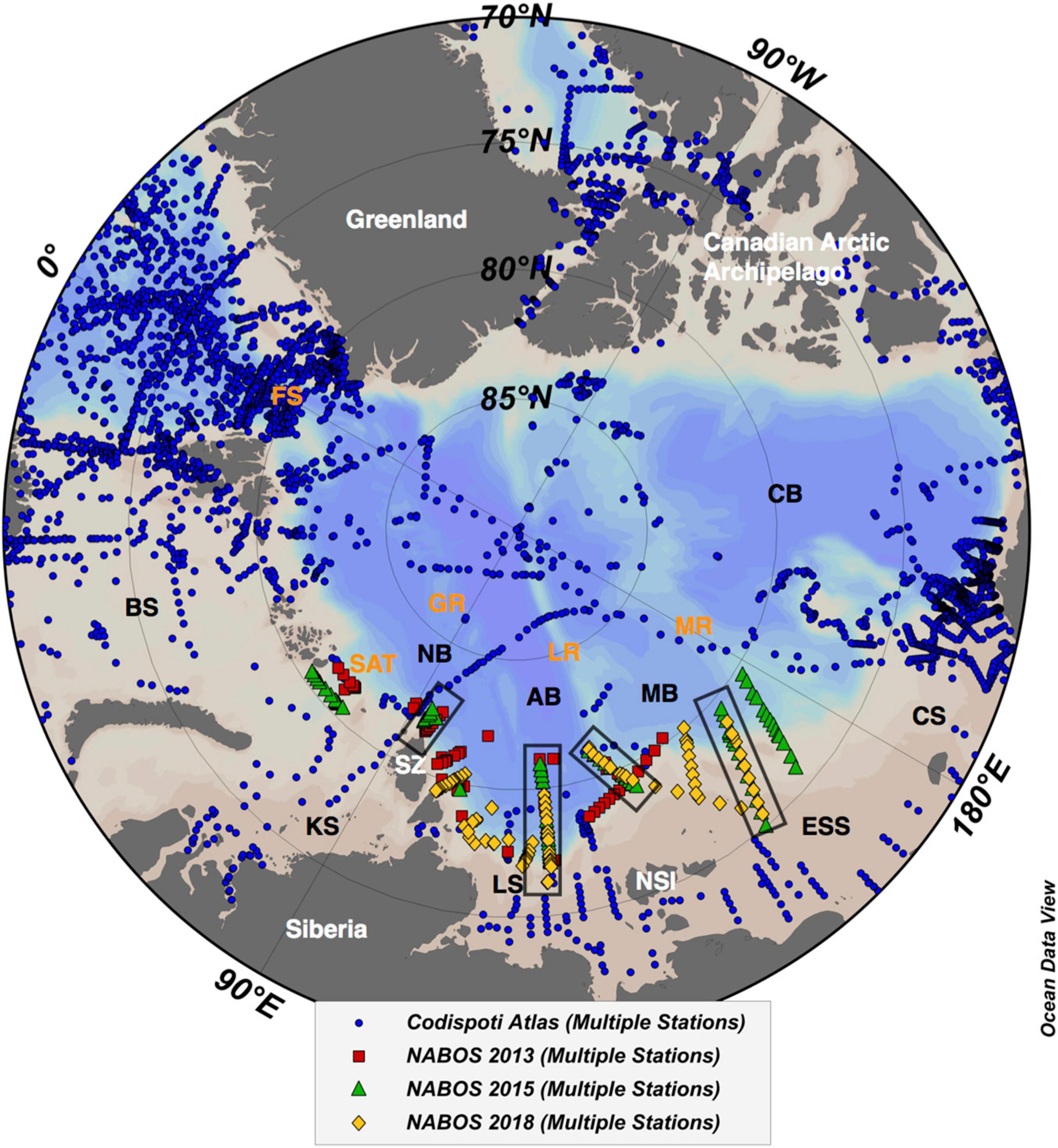
Figure 1. Locations of stations occupied during NABOS cruises conducted in 2013 (red squares), 2015 (green triangles), and 2018 (yellow diamonds) as well as the stations incorporated into the Codispoti et al. (2013) Nutrient Atlas (blue circles). Four, cross-slope transects that were re-occupied between 2013 and 2015 are highlighted by boxes. Bathymetric features are listed in orange: FS, Fram Strait; SAT, Saint Anna Trough; GR, Gakkel Ridge; LR, Lomonosov Ridge; MR, Mendeleyev Ridge. Islands (and other land masses) are listed in white: SZ, Severnaya Zemlya; NSI, New Siberian Islands. Deep basins and shelf seas are listed in black: NB, Nansen Basin; AB, Amundsen Basin; MB, Makarov Basin; CB, Canada Basin; BS, Barents Sea; KS, Kara Sea; LS, Laptev Sea; ESS, East Siberian Sea; CS, Chukchi Sea. Map created using Ocean Data View software, version 4.6.3 (Schlitzer, 2006).

FIGURE 2

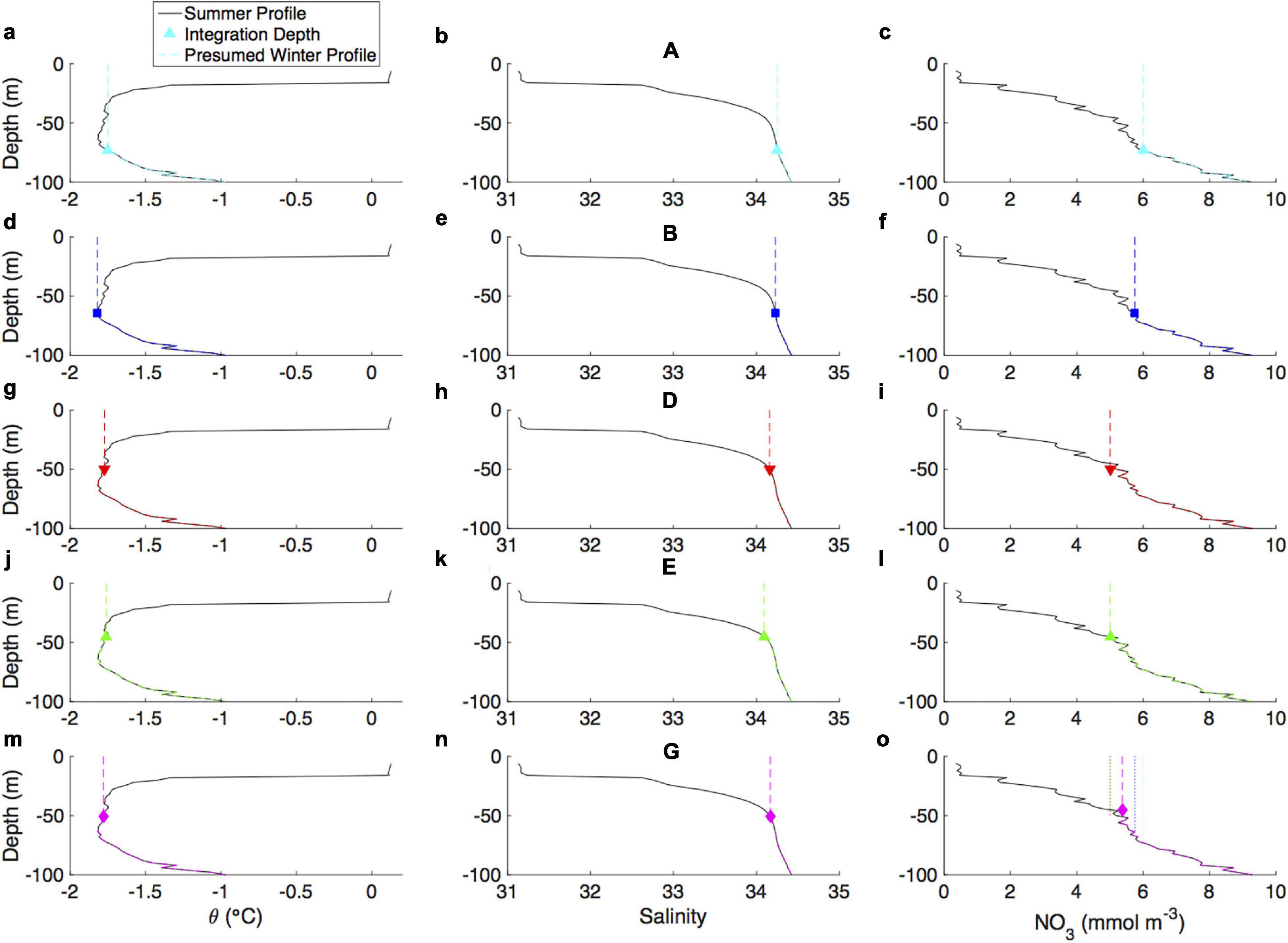
Figure 2. Vertical profiles of potential temperature (θ; left panels), salinity (middle panels), and nitrate (NO₃; right panels) in the top 100 m for a single station located along the Laptev Sea transect (∼80.2°N, ∼126°E) during the 2015 cruise. In each panel, the observed profiles are shown as solid black lines whereas the estimated integration depths from methods A, B, D, E, and G are shown as cyan triangles (a–c), blue squares (d–f), inverted red triangles (g–i), green triangles (j–l), and magenta diamonds (m–o), respectively. Presumed winter profiles are also shown as dashed lines. Net community production is computed by integrating the difference between the presumed winter and summer profiles between the surface and the estimated integration depth. The final panel (o) also shows the presumed winter nitrate profiles from all methods, for comparison.

Although winter data are still lacking, cruises of the Nansen and Amundsen Basins Observational System (NABOS) conducted in 2013, 2015, and 2018 provide high-resolution, sensor based profiles of nitrate, oxygen, beam attenuation, and chlorophyll fluorescence during late summer (August–September) to estimate NCP along transects crossing the continental slopes of the Kara, Laptev, and East Siberian Seas into the Amundsen and Makarov Basins: data-sparse regions identified in the Codispoti et al. (2013) study. We further exploit these high-resolution vertical profiles to determine whether assumptions made in previous studies regarding the integration depths and pre-bloom nitrate concentrations to calculate NCP are valid in slope and shelf regions. We also seek alternative methods to estimate these two necessary parameters as a contrast to assuming constant values for these parameters (as done in Codispoti et al., 2013) and assigning values to these parameters from estimates of the WML depth using summer temperature (and salinity) profiles (as done in Uflsbo et al., 2014). Finally, we assess spatial and temporal variability in NCP along the Siberian continental slope via comparisons along transects that were re-occupied during the three cruises.

Materials and Methods

Hydrographic stations were occupied during three cruises aboard the Russian Research Vessels Akademik Federov (2013) or Akademic Tryoshnikov (2015 and 2018) during August-September of each year (Figure 1). Cruises were conducted in partnership with the Arctic and Antarctic Research Institute (St. Petersburg, Russia) as well as various other international academic organizations (e.g., Alfred-Wegener Institute, Norwegian Polar Institute, Pusan National University of Korea).

Measurements

During each cruise, the instrument suite consisted of an SBE9plus CTD (conductivity-temperature-depth) equipped with dual temperature (SBE3) and conductivity (SBE4) sensors, dissolved oxygen sensor (SBE43), submersible pump (SBE5T), and digiquartz pressure sensor, a Benthos PSA-916 altimeter, WET Labs C-star transmissometer, WET Labs ECO-FLNTU deep chlorophyll and turbidity sensor, Biospherical PAR (photosynthetically active radiation) sensor (model QCP2350), and a Satlantic SUNA (Submersible Ultraviolet Nitrate Analyzer) Deep. Seawater samples were collected using a rosette carousel consisting of twenty-four Niskin bottles (10 L capacity) and analyzed for chlorophyll concentration, stable oxygen isotopes (δ¹⁸O), barium, dissolved oxygen, and nutrients (PO₄^3–, Si(OH)₄, NO₃^–, NO₂^–, and NH₄⁺) at regular depth intervals. Additional details describing the collection, analysis, and quality control procedures for water samples accompany the data sets on the NSF Arctic Data Center (see Section “Data Availability”).

Details describing operation and calibration of the SUNA instrument also accompany the data sets and are additionally available in the Supporting Information. Briefly, the SUNA instrument measures the ultraviolet absorbance of seawater across a 1-cm path length at a frequency of ∼0.9 Hz. The spectral data are aligned with the CTD measurements by synchronizing the two data streams in time. The temperature and salinity from the CTD are used to estimate the UV absorption due to bromide, which is subtracted from the total absorption to calculate the absorption due to nitrate (after a minor, baseline correction for dissolved organic matter) (Sakamoto et al., 2009; Alkire et al., 2010). The estimated nitrate concentrations are then corrected for potential instrument drift via linear regression(s) against a subset of nitrate concentrations determined from the seawater samples.

Dissolved oxygen concentrations measured by the SBE43 sensor were calibrated against concentrations determined from water samples on-board via the Winkler method using a Metrohm 888 Titrando and tiamo^® software allowing for automated (potentiometric) endpoint detection. Calibration coefficients were adjusted according to methods outlined in the Seabird Application Note No. 64-2 (2010 February). The precision of Winkler-determined dissolved oxygen concentrations was estimated to be 0.03 mL L^–1 (2013), 0.04 mL L^–1 (2015), and 0.02 mL L^–1 (2018) based on random replicates collected during each cruise.

Beam transmittance and the beam attenuation coefficient (cp) were calculated from measurements of the transmissometer using factory calibration coefficients provided by the manufacturer. Uncalibrated, chlorophyll fluorescence measurements (volts) are reported for qualitative purposes only.

Estimates of Net Community Production

Net community production was estimated via trapezoidal integration of the difference between an assumed pre-bloom nitrate concentration and nitrate concentrations measured in situ using the SUNA between the surface and the integration depth (Eq. 1):

$\text{NCP}\left(\text{mmol}{\text{m}}^{-2}\right)={\int }_0^{Zint}\left(N_{pre}-N_{meas}\right)\mathit{d}z\cdot R(1)$

where Z_int = integration depth, N_pre = pre-bloom nitrate concentration, N_meas = observed nitrate concentration (i.e., summer profiles), and R = Redfield ratio (106/16).

Note that vertical profiles of all sensor-based measurements were bin-averaged to 2 m resolution, in order to best match the sampling frequency of the SUNA. In addition, any negative nitrate concentrations were set equal to zero prior to integration and the top 0–6 m of the water column were assumed to be homogeneous. These estimates of nitrate uptake were converted to units of carbon production (g C m^–2) using the Redfield ratio 106:16 to facilitate comparison with previous studies (Codispoti et al., 2013; Uflsbo et al., 2014).

Five different estimates of NCP (A, B, D, E, and G) that utilized different methods of calculating or assigning the integration depth and/or pre-bloom nitrate concentration are compared in this study. An example comparison of the integration depths and pre-bloom nitrate concentrations estimated by these methods is provided in Figure 2. The A estimates of NCP were calculated via assigning a pre-bloom nitrate concentration of 6 mmol m^–3 and the integration depth was assigned as the depth where the nitrate concentration was equal to the assigned pre-bloom nitrate concentration at each station (Figures 2a–c). B estimates of NCP were calculated employing the integration depth and nitrate concentration associated with the winter mixed layer depth (Figures 2d–f). The D estimates were computed by assigning an integration depth of 50 m and a pre-bloom nitrate concentration of 5 mmol m^–3 (Figures 2g–i). E estimates were computed in a similar manner to the A estimates; however, the assigned pre-bloom nitrate concentration was set to 5 mmol m^–3 (Figures 2j–l). G estimates were calculated by determining the point at which vertical profiles of nitrate concentrations and percent oxygen saturations cross to determine the integration depth and pre-bloom nitrate concentration (Figures 2m–o).

Winter Mixed Layer (Zwml)

The depth of the winter mixed layer was estimated by determining the minimum potential temperature below the surface mixed layer (estimated using a 0.02 kg m^–3 density difference from the average potential density over 0–10 m) (Figure 2d). This method was introduced by Rudels et al. (1996) to identify the remnant winter mixing layer in the Nansen and Amundsen Basin of the Arctic Ocean using summer CTD profiles. Subsequent studies have adopted this method for determining the winter mixed layer depth (Zwml) as the maximum depth for integrating net community production (e.g., Uflsbo et al., 2014) as this remnant winter mixed layer likely reflects the hydrographic conditions (e.g., temperature, salinity, nitrate concentration) assumed to be homogeneous throughout the mixed layer during winter months.

Although this may be a preferred method by which to compute NCP in the absence of winter data, it was not always possible to determine an unambiguous Zwml, particularly in the ESS and on the shelves where bottom depths < 200 m. In fact, Zwml could not be reliably determined at most of the stations occupied east of ∼150°E during the 2015 cruise; therefore, alternative methods to estimate the integration depth and pre-bloom nitrate concentration at each station were sought.

Depths of Targeted Nitrate Concentrations (ZN5 and ZN6)

The bin-averaged nitrate profiles were linearly interpolated to determine the depth at which the nitrate concentration was equal to 5 mmol m^–3 (ZN5) and 6 mmol m^–3 (ZN6). These depths were taken as integration depths to compute NCP under scenarios E and A, respectively. As such, these NCP estimates allow for the integration depth to vary freely whereas the pre-bloom nitrate concentrations are prescribed. These scenarios assume winter mixing penetrates to approximately the depths of the 5 or 6 mmol m^–3 levels and the water column is homogenized at a pre-bloom nitrate concentration associated with the corresponding horizon (Figures 2c,l). These scenarios were included because Codispoti et al. (2013) determined pre-bloom nitrate concentrations of 5 and 6 mmol m^–3 were appropriate in areas that corresponded closest to the NABOS study area (i.e., ESS + Laptev Northern and Southern subregions).

Depth of Nitrate and Dissolved Oxygen Intersection (Zsect)

An alternate method was sought to determine integration depths and pre-bloom nitrate concentrations that allows both parameters to vary freely (as is the case for B). To this end, the depth at which vertical profiles of nitrate and dissolved oxygen cross each other was set as the integration depth and the associated nitrate concentration was taken as the pre-bloom nitrate concentration at each station. The reasoning behind this choice was to locate a depth below the layer within which nitrate concentrations were zero and above (or within) the nitracline and oxycline as an approximation of the maximum depth of winter mixing and/or nutrient uptake by phytoplankton.

The depth of intersection (Zsect) was determined for each station as follows. First, the vertical profiles of nitrate and oxygen were truncated to include only depths between the surface mixed layer and 100 m. The maximum winter mixed layer depth observed over the study was 88 m and it was determined highly unlikely that photosynthetically driven nitrate uptake would occur below 100 m. The truncated nitrate and oxygen profiles were then standardized by subtracting their respective means and dividing by the standard deviations. This standardization allowed for the nitrate and oxygen profiles to be plotted on the same axis, minimizing uncertainties in the determination of the intersection point associated with attempting to match up nitrate and oxygen profiles with substantially different concentration ranges. A test metric was calculated by subtracting the standardized oxygen profile from the standardized nitrate profile and the minimum absolute value of this metric was taken as the intersection point. Figures depicting these steps are provided in the Supplementary Figure 1.

The profiles were truncated as the inclusion of shallower and/or deeper portions of the profile, respectively, decrease or increase the mean values used in the standardization and therefore alter the estimation of the intersection depth. As we expect the integration depth to be deeper than the SML and no greater than the deepest WML observed, we argue that the depth interval chosen for the calculation is justified. However, the sensitivity of the intersection depth calculation to the chosen depth interval was tested. Extending the included depth interval to include shallower observations (0–100 m) did not significantly change the estimated intersection depth (mean difference of −2 ± 14 m for the three cruise years). However, the inclusion of measurements to a depth of 120 m yielded intersection depths deeper by an average of 10 ± 15 m (0–120 m) and 5 ± 15 m (SML to 120 m). Extending the range further to 0–200 m resulted in an even higher, but more variable, increase in the intersection depth: a mean difference of 29 ± 25 m. Given these results, one might expect the truncation adopted in this study (SML to 100 m) to potentially underestimate the integration depth (assumed equivalent to Zwml) whereas utilizing a larger section of the profile may overestimate it. Additional work is needed to further refine this technique.

The intersection depths determined using this algorithm were visually checked for accuracy. In most cases (84%), the algorithm returned an intersection depth within ±3 m of the visually determined intersection using the standardization method. In the remaining 16% of cases (n = 38), the visually determined intersection depth differed from the algorithm by between −13 and +56 m. These cases resulted from either the limited vertical resolution of the measurements (2 m) or multiple intersections of the two profiles. Whenever multiple intersections were encountered, the shallowest intersection was taken for Zsect.

We briefly note that attempts were also made to determine integration depths by estimating inflection points in the nitrate, dissolved oxygen, and percent oxygen saturation profiles. The reasoning behind such an attempt was the potential ability to determine integration depths using only a single, biogeochemical variable. However, there were two issues with this approach. First, estimation of the inflection point requires fitting a 3rd degree polynomial to the profiles; this fitting procedure does not always produce a satisfactory fit (low correlation coefficient) and the depth interval used in the fit (e.g., 0–100 m, 0–200 m, 20–300 m, 0–1000 m) highly influences the estimated inflection point (or in some cases, multiple inflection points). Second, the inflection points that were determined separately from nitrate, dissolved oxygen, and percent oxygen saturation did not typically agree. Therefore, rather than choose a variable that may be more appropriate for estimating the integration depth, we decided to combine information from the nitrate and oxygen profiles to determine the “optimal” integration depth taken as the intersection point.

Meteoric Water and Sea Ice Meltwater Inventories

Pairs of salinity and δ¹⁸O measurements determined from collected water samples were used to calculate fractional contributions of meteoric water (MW) and net sea ice meltwater (SIM) to each station using methods outlined in Alkire et al. (2015). Briefly, a seawater sample collected from the NABOS study area is composed of a combination of three water types: MW, SIM, and Atlantic water (ATL). Assuming certain endmember values of salinity and δ¹⁸O accurately characterize each of these water types, one can use a coupled set of equations to calculate the fractional contributions of each water type to the collected sample (Eqs 2–4):

$\begin{array}{c}{\text{S}}_{\text{MW}}\times {\text{f}}_{\text{MW}}+{\text{S}}_{\text{SIM}}\times {\text{f}}_{\text{SIM}}+{\text{S}}_{\text{ATL}}\hfill \\ \times {\text{f}}_{\text{ATL}}={\text{S}}_{\text{meas}}\hfill \end{array}(2)$

$\begin{array}{c}{\mathrm{\delta }}^{18}{O}_{\text{MW}}\times f_{\text{MW}}+{\mathrm{\delta }}^{18}{O}_{\text{SIM}}\times f_{\text{SIM}}\hfill \\ +{\mathrm{\delta }}^{18}{O}_{\text{ATL}}\times f_{\text{ATL}}={\mathrm{\delta }}^{18}{O}_{\text{meas}}\hfill \end{array}(3)$

${\text{f}}_{\text{MW}}+{\text{f}}_{\text{SIM}}+{\text{f}}_{\text{ATL}}=1(4)$

In practice, there are uncertainties associated with the assigned endmember values and this can result in errors to the water type analysis. Therefore, a range of likely endmember values (based on the literature) is applied to the analysis by computing 1,000 different water type fractions for each sample (i.e., the same salinity, δ¹⁸O pair) using a set of endmember values that have been randomly selected from within the specified ranges. For the NABOS data set, the endmember ranges were assigned as follows: S_MW = 0; −22 ≤δ¹⁸O_MW ≤−18‰; 2 ≤S_SIM < 8; −2 ≤δ¹⁸O_SIM ≤0.3‰; 34.85 ≤S_ATL ≤35; 0.25 ≤δ¹⁸O_ATL ≤0.35‰. The averages of the 1,000 iterations were taken as the most likely MW, SIM, and ATL fractions for each sample and the associated standard deviation taken as an estimate of the uncertainty. The median uncertainties for MW, SIM, and ATL fractions calculated for the three NABOS cruises were 0.003, 0.004, and 0.002, respectively.

We note that Pacific water influence was not taken into account when calculating these water type fractions. In this region of the Arctic, contributions from Pacific water are expected to be minimal, except in the eastern and central regions of the ESS (Semiletov et al., 2005). In fact, it was argued that Pacific halocline waters were present in the eastern part of the ESS in 2015, observed along the easternmost transect of the NABOS study area in that year (Alkire et al., 2019). Ignoring this contribution will result in an overestimation of MW fractions and a possible underestimation of SIM fractions along this transect. However, such potential biases do not greatly affect the results of this study.

Positive inventories of MW and SIM were computed for each station over a depth range of 0–50 m. First, any negative MW or SIM fractions were set equal to zero; this step was meant to exclude any brine (negative SIM fractions) and erroneous MW fractions (all MW fractions should be positive) so that the resulting inventories would approximate the seasonal (summer) inputs of sea ice meltwater, precipitation, and river runoff to the upper water column. These adjusted fractions were interpolated onto a regular, 10 m grid (near-surface, 10, 20, 30, 40, 50 m; matching the target sampling intervals) and integrated.

Data Availability

All data collected by the University of Washington and University of Alaska Fairbanks are available online through the NSF Arctic Data Center (Polyakov, 2016a,b; Alkire, 2019; Alkire and Rember, 2019).

Hydrographic Setting and Background

The top 0–300 m of the water column in the eastern Arctic Ocean, considered here to include the Nansen and Amundsen Basins as well as the Siberian continental slope, generally consists of three layers: a surface mixed layer, a halocline layer, and a deeper Atlantic layer. The surface mixed layer may be warm or cold during late summer/early fall, depending on the position of the sea ice edge; ice-free waters generally exhibit warmer temperatures due to solar insolation whereas as ice covered waters (or recent melting) are associated with colder temperatures. The median depth of the surface mixed layer was 12 ± 5 m across the study region and exhibited lower salinities compared to underlying waters, zero (or near zero) nitrate concentrations, and relatively high oxygen saturation (e.g., see Figure 3). Below the surface layer, the salinity increases rapidly with depth whereas temperature typically remains close to the freezing point; this is often called the cold halocline layer and its presence is important for separating the cold and fresh surface waters (and overlying sea ice) from warm and saline Atlantic waters at depth (Polyakov et al., 2020b). Similar to salinity, nitrate concentrations also increase with depth (Figures 3c,i) whereas oxygen saturations decrease (Figures 3d,j).

FIGURE 3

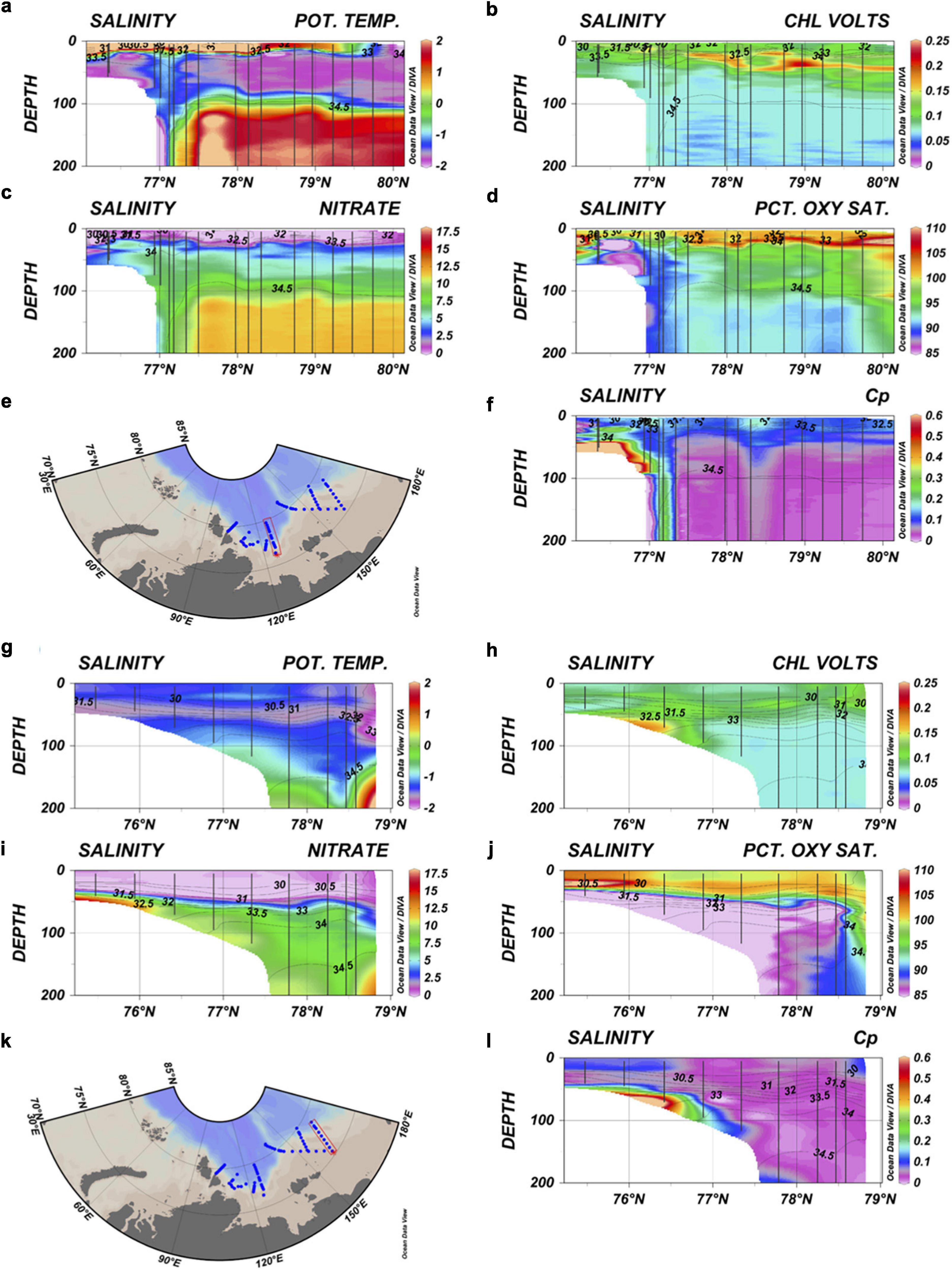
Figure 3. Cross-slope sections of (a) potential temperature [°C], (b) raw chlorophyll fluorescence [V], (c) nitrate [mmol m^–3], (d) percent oxygen saturation [%], and (f) the beam attenuation coefficient [Cp, m^–1] for the Laptev Sea transect (∼126°E) occupied in 2018. The associated map is provided in panel (e). Panels (g–l) depict the same variables for the East Siberian Sea transect (∼165°E), also occupied in 2018. Plots were created using Ocean Data View software, version 4.6.3 (Schlitzer, 2006). The data are displayed using DIVA gridding with automatic length scales enabled.

Below the halocline, warm and saline Atlantic waters that have entered the Arctic via Fram Strait typically reside between ∼100 and 450 m. This Fram Strait Branch (FSB) of Atlantic water circulates cyclonically around the Arctic along the continental slopes and mid-ocean ridges via bathymetric steering (Rudels et al., 1996, 2004). On the slope, there is an obvious front in potential temperature (as well as oxygen and nitrate) that separates the FSB Atlantic water (warm and replete in both nitrate and oxygen) from slope/shelf waters that are comparatively colder and generally depleted in oxygen (Figure 3). Farther inshore, bottom waters on the shelf can exhibit oxygen saturations <85% and nitrate concentrations in excess of 10 mmol m^–3 due to the respiration of organic matter sinking to the sediments (Anderson et al., 2011, 2013). In addition to higher nutrient concentrations, chlorophyll fluorescence (Figure 3b), turbidity, and beam attenuation (Figure 3f) are often higher in near-bottom waters due to sediment resuspension and/or turbidity currents.

Moving from west to east along the Siberian continental slope, surface waters become fresher (decreasing salinity) and the halocline becomes thicker. For example, contrasting the Laptev Sea transect (∼126°E; Figures 3a–f) and ESS transect (∼160°E; Figures 3g–l) shows that the S = 34 isohaline deepens from ∼50 m in the west to ∼100 m in the east. This decrease in salinity results from the offshore advection of Siberian shelf waters in the vicinity of the Lomonosov and Mendeleev Ridges (Bauch et al., 2009). Shelf waters receive large freshwater inputs from river discharge (presumed low in NO₃^–) (Macdonald et al., 1987, 2015; Holmes et al., 2012; McClelland et al., 2012, 2014) and the movement of these river-laden waters across the slope and into the deep basins increases stratification and maintains the permanent halocline (Steele and Boyd, 1998). Farther eastward in the ESS, Pacific waters that have entered the Arctic via Bering Strait can be encountered (Semiletov et al., 2005; Alkire et al., 2019). Pacific waters entering the ESS from the Chukchi Sea can be characterized by higher values of the NO parameter, where NO = (9×[NO₃^–]) + [O₂] (Broecker, 1974), compared to Siberian shelf and Atlantic waters flowing eastward (Alkire et al., 2019). During years characterized by Pacific influence, the surface sediments of the eastern ESS primarily reflect organic matter derived from autotrophic production (algal cells) whereas those of the western ESS, outside of the Pacific influence, reflect terrigenous sources (Semiletov et al., 2005).

In fall and winter months (November–May), a combination of cooling, wind stress, and brine rejection from ice formation deepens and homogenizes the surface mixed layer; depending on the depth of mixing and the local stratification this process replenishes nitrate and other nutrients in the euphotic layer where they can be utilized by phytoplankton the following spring (Macdonald et al., 1987). Arctic winters are dark and most of the surface area is covered by sea ice, preventing photosynthesis. Typically starting in May and continuing through June or July, the Arctic thaws and the melt back of the snow cover and breakup and thinning of ice alleviates light limitation and stimulates algal production both within the sea ice and underlying water column (Carmack and Wassmann, 2006). The spring bloom exhausts nitrate in the surface layers and the continued melt of the ice as well as the spring flood of river runoff from the continents increases the stratification such that higher nutrient concentrations at depth are mostly isolated from sunlit surface waters. Stratification is particularly strong on the broad and shallow Siberian shelves and organic matter originating from autotrophic production (Redfield C:N ratio) as well as riverine sources (high C:N ratio) is remineralized in the sediments and released to bottom waters (Carmack et al., 2006; Macdonald et al., 2015). Suspended sediments delivered by the rivers increases the turbidity on the shelves and may impede photosynthesis as light penetration is reduced. Similarly, the resuspension of bottom sediments on the shelf and slope can increase the turbidity in bottom and near bottom waters (Macdonald et al., 2015).

During the late summer period (late August to early October) when the NABOS cruises were conducted, biological production was primarily derived from recycled nutrients (i.e., remineralized production) as nitrate concentrations throughout the topmost 0–30 m were mostly equal to zero (Figures 3c,i). Subsurface maxima in chlorophyll fluorescence (Figures 3b,h) and oxygen saturation (Figures 3d,j) were also evident across the study area, indicative of continued, but diminished, photosynthesis despite the apparent lack of nitrate in surface waters.

Based on the maximum WML depth of <100 m determined for the study region, we are primarily concerned with the top 0–100 m of the water column for the calculation of NCP. However, the fronts over the continental slope, increasing influence of river-laden shelf waters moving eastward, potential intrusion of Pacific waters into the ESS, and persistence of nutrient-replete and oxygen-deplete bottom waters over shallow shelves all complicate the estimation of NCP. For example, assigning a constant integration depth of 50 m may encounter shelf bottom waters in shallower regions that might be preferable to exclude from the calculation. In contrast, the assignment of a specific isopycnal as the bottom boundary of integration for NCP calculations will result in a sizeable increase in the depth range at eastern stations compared to western stations. Additional complexities arise as NCP is expected to exhibit interannual and spatial variability due to changing environmental conditions (river discharge, sea ice melt, wind forcing, the timing and duration of the open water period, etc.). The comparison of methods A, B, D, E, and G are meant to help address these concerns and determine how impactful such dynamics might be on NCP calculations using the seasonal nitrate drawdown approach.

Results

Integration Depth Estimates

Overall, the mean estimates of Zwml (50 ± 11 m), Zsect (47 ± 10 m), ZN6 (54 ± 16 m), and ZN5 (44 ± 12 m) were quite similar. However, station-to-station comparisons differed considerably. Simple linear regressions (Supplementary Figure 2) indicated poor correlations among NCP estimates as R² values were mostly below 0.1.

Winter mixed layer depths (Zwml) did not exhibit much spatial or temporal variability; however, some shallower depths (<40 m) were observed north of Severnaya Zemlya and a few deeper depths (>60 m) observed in the southern Laptev Sea (Figures 4a–c). More variations were observed in the depths of the 5 mmol m^–3 NO₃^– horizon (ZN5) as depths tended to be shallower (<40 m) west of ∼120°E and somewhat deeper (40–60 m) to the east (Figures 4j–l). ZN5 depths also exhibited some temporal variation along the Laptev Sea transect (∼126°E); ZN5 was somewhat shallower along the southern half of the transect in 2015 and 2018 compared to 2013. The Lomonosov Ridge transect (∼145°E) also exhibited somewhat shallower ZN5 depths in 2015 compared to 2013 and 2018. Similar variations were observed in the ZN6 distributions (Figures 4g–i), though the depths were greater overall. One difference of note between the ZN5 and ZN6 distributions was a deepening of ZN6 toward > 80 m on the northward ends of the Lomonosov Ridge and ESS transects in 2018 that was not apparent in the ZN5 distribution. The Zsect distribution (Figures 4d–f) exhibited little spatial variability in 2013; however, the 2015 distribution indicated a small longitudinal gradient, where depths were somewhat greater (∼60 m) in the ESS compared to the Laptev Sea and Lomonosov Ridge regions (40–50 m). There were also a few stations with surprisingly shallow integration depths on the eastern side of the St. Anna Trough. In 2018, integration depths were relatively shallow over most of the study area, but particularly along the southern portions of the slope in the Laptev Sea and ESS as well as the western flank of the Lomonosov Ridge.

FIGURE 4

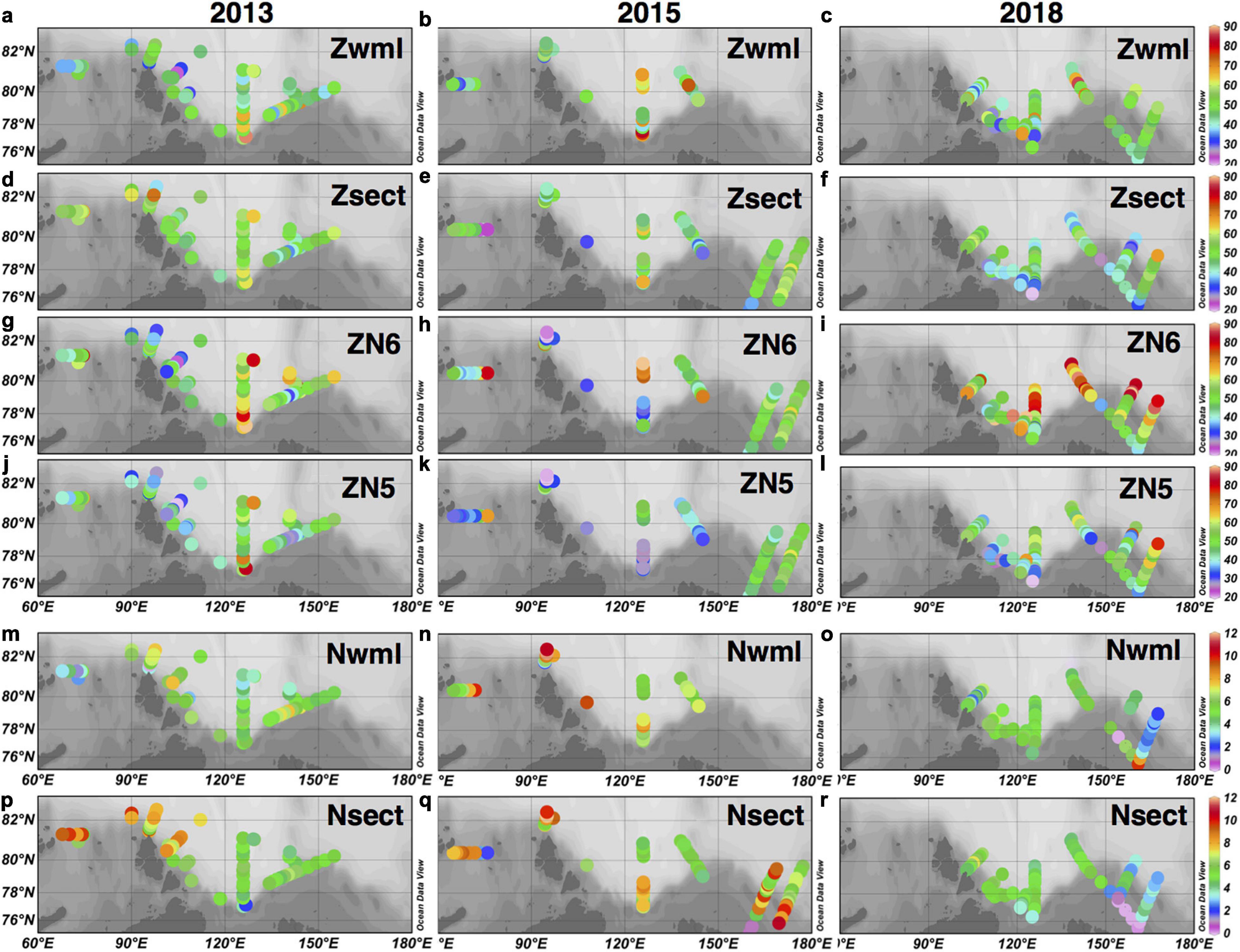
Figure 4. Maps of integration depths and pre-bloom nitrate concentrations estimated using the five methods (A, B, D, E, and G). Each row corresponds to a different integration depth or pre-bloom nitrate concentration estimate whereas each column corresponds to a different cruise year: 2013 (left column), 2015 (middle column), and 2018 (right column). The first row (a–c) shows the distribution of the winter mixed layer depths (Zwml), the second row (d–f) shows the NO₃-O₂ intersection depths (Zsect), the third row (g–i) shows the depths of the NO₃ = 6 mmol m^–3 horizon (ZN6), the fourth row (j–l) shows the depths of the NO₃ = 5 mmol m^–3 horizon, the fifth row (m–o) shows the pre-bloom NO₃ concentration associated with the winter mixed layer depth (Nwml) and the last row (p–r) shows the NO₃-O₂ intersection NO₃ concentration.

Overall, the comparisons suggest that, despite the similarity in the central values/medians of the different integration depth estimates, the spread/variability among these estimates was quite different. As a result, station-to-station comparisons did not agree well, so that each method yielded a distinctly different result.

Pre-bloom Nitrate Concentration Estimates

Averages of the two freely varying estimates of the pre-bloom nitrate concentration, Nwml (5.4 ± 1.8 mmol m^–3) and Nsect (5.7 ± 2 mmol m^–3) were quite similar; however, a simple linear regression of Nwml vs. Nsect (Supplementary Figure 3) suggested a very weak correlation (R² = 0.1).

In 2013, Nwml (Figures 4m–o) and Nsect (Figures 4p–r) spatial distributions generally agreed to the east of ∼120°E; however, west of this longitude, Nsect concentrations were consistently higher than Nwml, especially in the St. Anna Trough region and just offshore of Severnaya Zemlya. Nsect and Nwml also generally agreed in 2015 except in the St. Anna Trough region: Nwml concentrations indicated an increase moving west to east across the trough whereas the Nsect concentrations exhibited the opposite trend. It was interesting to note that both Nsect and Nwml exhibited higher concentrations on the southern half of the Laptev Sea transect in 2015 compared to 2013. Winter mixed layers could not be determined with any confidence east of 150°E for the 2015 stations, but the Nsect distribution indicated substantial variability with highest concentrations over the slope and on the northern end of the 165°E transect.

In 2018, the Nsect and Nwml distributions looked quite similar except for a shallow area over the shelf on the eastern flank of the Lomonosov Ridge where Nwml concentrations ranged between 5 and 10 mmol m^–3 but Nsect concentrations were zero. Note that the Nsect concentrations decreased markedly in the ESS between 2015 and 2018.

Net Community Production Estimates

Average NCP estimates from the five methods overlapped, with the lowest estimates from the E (11.9 ± 4.2 g C m^–2) and D (11.7 ± 3.9 g C m^–2) methods, followed by method B (12.7 ± 4.9 g C m^–2), G (14.2 ± 7.2 g C m^–2), and A (15.8 ± 4.9 g C m^–2). Simple, linear regressions comparing the methods (Supplementary Figure 4) indicated that the NCP from methods D and E were essentially interchangeable (slope = 0.9, intercept = 0.7, R² = 0.98). Strong correlations (R² > 0.9) were also observed between method A vs. E and D, with offsets (intercepts) of ∼2 g C m^–2. All other regressions suggested little to no correlation (R² < 0.1).

Before the spatial distributions of NCP are discussed, the impacts of freshwater inputs on the seasonal nitrate uptake calculation must first be taken into account.

Assessing the Impact of Meteoric Water and Sea Ice Meltwater on Net Community Production

The calculation of NCP estimates presented in Eq. 1 ignores potential contributions from outside water masses that can effectively lower the nitrate concentration without contributing to production. For example, river runoff released to the shelves and melting of the sea ice cover during spring and summer may dilute/reduce nitrate inventories in the water column prior to (or during) the spring bloom. Most studies do not have the measurements required to estimate the potential impact of freshwater sources on NCP calculations and ignore the effect on NCP estimates based on comparisons of summer vs. winter nitrate stocks. The requisite data for estimating MW and SIM fractions were collected for this study; however, it is not known what nitrate concentrations were characteristic of MW or SIM entering the water column in the NABOS study region as neither was measured. It is generally expected that nitrate concentrations in sea ice meltwater and river runoff moving from the outer shelf to the slope would be relatively depleted of nitrate (Macdonald et al., 1987, 2015). It is also difficult to determine how much MW was delivered to the study region in winter vs. summer.

Due to these inherent uncertainties, we have assumed the nitrate concentration of both SIM and MW to be low (0.1 mmol m^–3) in order to estimate the maximum potential reduction on the NCP calculations. The differences to NCP calculations due to MW and SIM were calculated as follows: (1) adjust the integration depth to account for the inventories of MW and SIM (see Eq. 5); (2) calculate the adjusted, pre-bloom nitrate inventory (see Eq. 6); (3) calculate the unadjusted pre-bloom nitrate inventory (see Eq. 7); (4) subtract the difference between the unadjusted and adjusted nitrate inventories and convert to units of g C m^–2 (this is the effective reduction in NCP) and subtract this from the original NCP estimate (see Eq. 8).

${\text{Z}}_{\text{adj}}={\text{Z}}_0-{\text{MW}}_{\text{inv}}-{\text{SIM}}_{\text{inv}}(5)$

$\begin{array}{c}{\text{N}}_{\text{adj}}=({\text{Z}}_{\text{adj}}\times {\text{N}}_0)+({\text{MW}}_{\text{inv}}\times 0.1)\hfill \\ +({\text{SIM}}_{\text{inv}}\times 0.1)\hfill \end{array}(6)$

${\text{N}}_{\text{inv}}={\text{Z}}_0\times {\text{N}}_0(7)$

$\begin{array}{c}{\text{NCP}}_{\text{adj}}=\text{NCP}-({\text{N}}_{\text{inv}}-{\text{N}}_{\text{adj}})/1000\hfill \\ \times (106/16)\times 12\hfill \end{array}(8)$

where Z_adj and N_adj are the adjusted integration depth and pre-bloom nitrate inventory, respectively; Z₀, initial (unadjusted) integration depth; N₀, initial (unadjusted) pre-bloom nitrate concentration; N_inv, initial (unadjusted) pre-bloom nitrate inventory; MW_inv, meteoric water inventory; and SIM_inv, sea ice meltwater inventory. These calculations essentially reduce (adjust) the pre-bloom nitrate inventory for the inputs of MW and SIM containing near-zero nitrate inventories.

These calculations were used to adjust the five different NCP estimates and the histograms of both unadjusted/initial (red bars) and adjusted (blue bars) NCP are plotted in Figure 5. The differences in the NCP estimates after adjustment for MW and SIM influence amounted to a median reduction in NCP by ∼2 g C m^–2 (or ∼10%); however, maximum differences were as large as ∼4 g C m^–2 for methods A-E and up to ∼8 g C m^–2 for method G (see Supplementary Figure 5). Overall, the variability in the different NCP estimates was unaffected; however, the adjusted NCP estimates did tend to reduce the number of higher NCP values across the five methods.

FIGURE 5

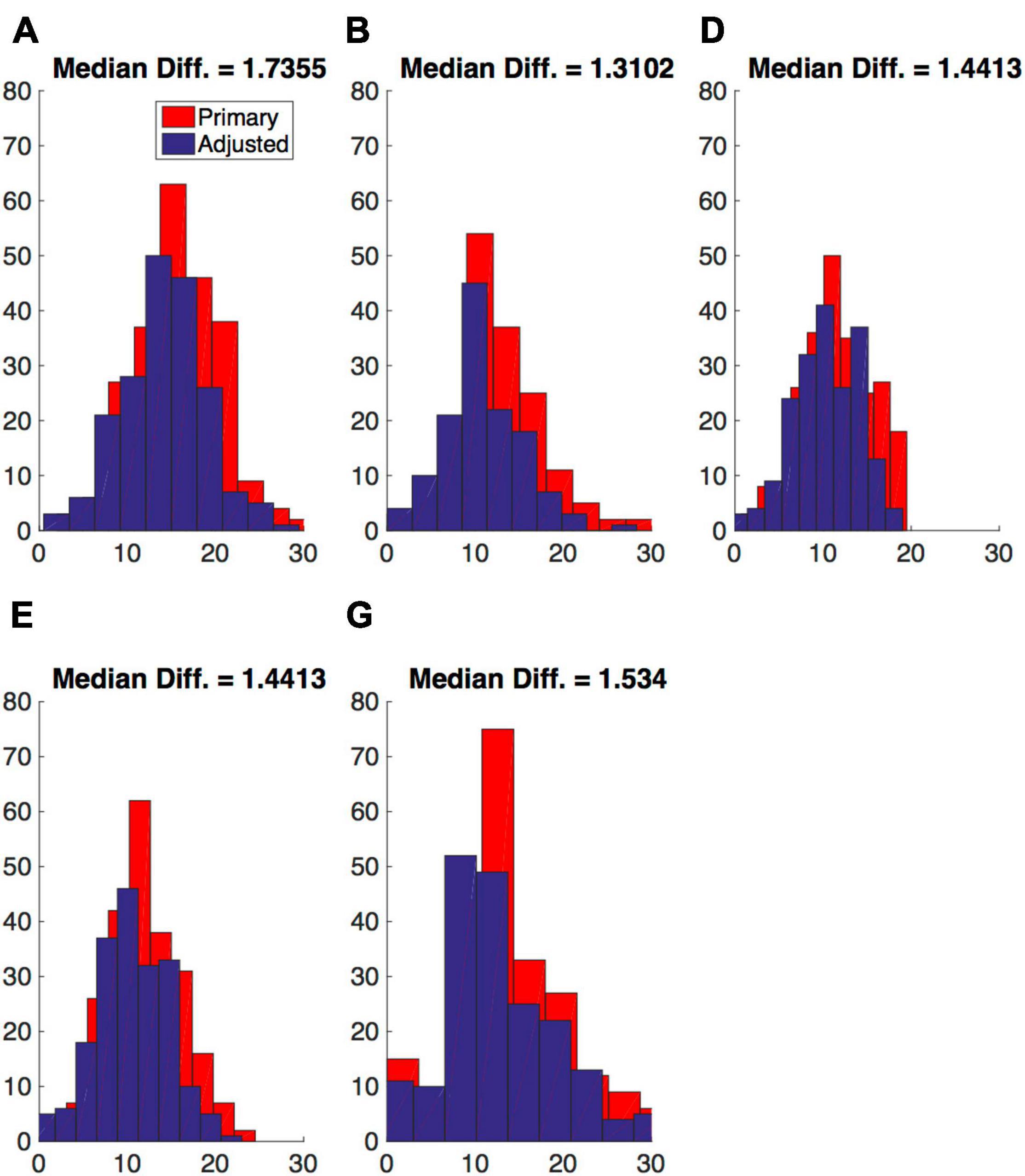
Figure 5. Histograms comparing estimates of net community production (NCP) using the five methods (A, B, D, E, and G) before (red bars) and after (blue bars) adjustment for the impact of meteoric water and sea ice meltwater on nitrate inventories. The median differences between the unadjusted (primary) and adjusted NCP estimates are given above each panel.

The differences in the NCP estimates reflect the maximum possible adjustment; the impact of MW and/or SIM influence may be smaller if they are associated with higher nitrate concentrations or enter the study area after the majority of the production has occurred. Therefore, the adjustments presented provide upper limits on the impacts of low-nutrient, freshwater inputs. Additionally, some NCP estimates are lost in the process as the necessary δ¹⁸O data to compute adjustments were not collected at every station. Despite these drawbacks, the differences between adjusted and unadjusted NCP estimates had significant linear correlations with latitude (Supplementary Figure 6) and longitude (Supplementary Figure 7), due to similar relationships between latitude and longitude and the meteoric water inventory (generally increased with increasing longitude and decreasing latitude; see Supplementary Figure 10). We have therefore decided to adopt these adjustments in our subsequent analyses of the NCP estimates.

It should be briefly noted that the adjusted NCP estimates expressed similar spatial and temporal variability as the unadjusted estimates (with a few exceptions) and the correlation among NCP estimates did not improve after the adjustments were made. For comparison, maps of unadjusted NCP estimates are provided in the Supporting Information (Supplementary Figure 11).

Comparing Net Community Production Across Transects

The majority of NCP estimates ranged between 5 and 30 g C m^–2, but there were some lower (near zero) and higher estimates (≥30 g C m^–2) observed over the study period. In general, higher NCP estimates were determined using the A and G methods compared to those estimated from B, D, and E methods (Figure 6). There was no obvious gradient or trend in NCP with respect to latitude under any method, but there were some longitudinal differences that recommended a regional analysis to better understand comparisons among the integration depths, pre-bloom nitrate concentrations, and NCP estimates from the different methods.

FIGURE 6

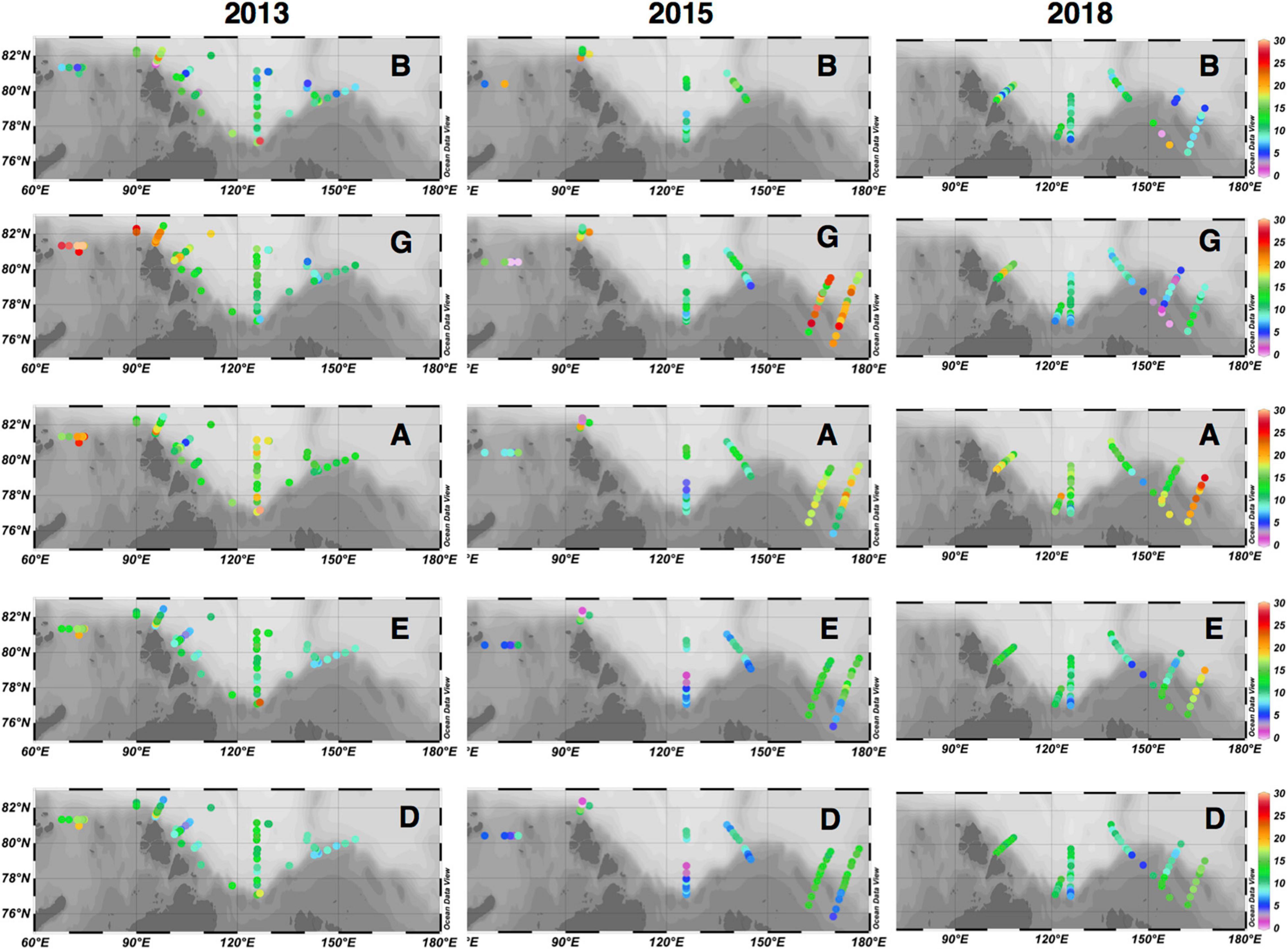
Figure 6. Maps of net community production estimates, after adjustment for meteoric water and sea ice meltwater influences, using the five methods (B, top row; G, second row; A, third row; E, fourth row; and D, bottom row) for each cruise year: 2013 (left panels), 2015 (middle panels), and 2018 (right panels). Colorbars are equivalent for all panels, with ranges set between 0 (cooler colors) and 30 (warmer colors) in units of g C m^–2.

In order to quantitatively assess both spatial and temporal variations, we examined the mean NCP estimates from four cross-slope (S-N oriented) transects that were re-occupied during the three cruises (see Figure 1 and Table 1). Comparisons among transect averages within a given cruise year provides a quantitative method to assess spatial variability whereas comparisons across cruises provides a sense of the temporal variations in NCP across the study region. We briefly note that the general patterns and drawn conclusions discussed in this section remain, for the most part, unchanged if the unadjusted NCP estimates are evaluated. A table listing the means and 95% confidence intervals of the unadjusted NCP estimates is provided in the Supporting Information (Supplementary Table 1).

TABLE 1

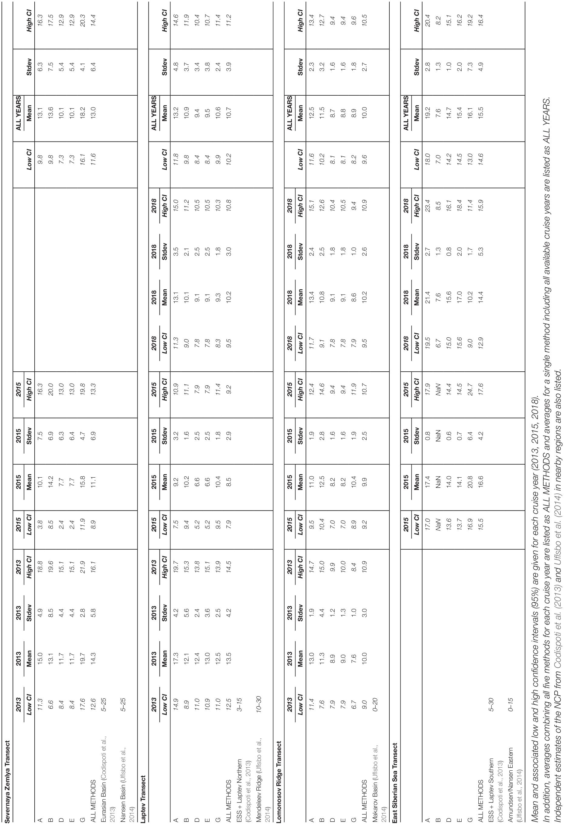
Table 1. Mean estimates of net community production from the five different methods (A, B, D, E, and G), averaged along the transects (Severnaya Zemlya, Laptev Sea, Lomonosov Ridge, and East Siberian Sea) outlined in Figure 1.

Severnaya Zemlya Transect

In 2013, the NCP estimated from method G was significantly higher than those estimated from methods D and E (all other NCP estimates were statistically indistinguishable). It was also notable that the standard deviations in NCP estimates using method G were the lowest of all five estimates whereas those from method B were highest. In 2015, all five NCP estimates were statistically indistinguishable, but the NCP computed from method G had the highest mean and the lowest standard deviation. Comparing the different methods between cruise years (2013 and 2015), there was no significant change in NCP from 2013 to 2015. However, if the two years are combined, method G exhibited the highest overall mean NCP (significantly higher than those from methods D and E) and lowest variance. Combining all methods across both years, the mean (±1 σ) NCP along this transect was 13 ± 6 g C m^–2.

Laptev Transect

In 2013, the mean NCP computed from method A was the highest of the five methods and statistically significantly higher than those computed from methods G and D (these methods exhibited the lowest standard deviations). All other NCP estimates were statistically indistinguishable. In 2015, the mean NCP from methods A, B, and G were similar and statistically higher than those from methods D and E (themselves statistically equivalent). During this year, the NCP from methods B and G exhibited the lowest standard deviations. In 2018, the NCP computed from method A was significantly higher than all other methods (which were statistically indistinguishable from each other); method G again exhibited the lowest standard deviation.

Comparing NCP estimates from individual methods across cruise years, methods A, D, and E exhibited a significant decrease between 2013 and 2015; in fact, the NCP from methods D and E exhibited a 50% decline between these years. The mean NCP of method A was the only one that increased between 2015 and 2018 (all others were statistically equivalent). However, the NCP from methods G, E, and D were all statistically significantly lower in 2018 compared to 2013. Overall, these results indicate a general decline in NCP along the Laptev transect between 2013 and 2018. This general trend was also evident when comparing annual means (combining the NCP across the five methods).

If individual methods are combined over all 3 years and compared, the NCP computed from method A was significantly higher than those estimated from methods D and E; all others were statistically indistinguishable. We note that only the estimate from method G exhibited a significantly lower NCP than that along the Severnaya Zemlya transect. When all NCP estimates are combined (across methods and cruise years), the mean NCP was 11 ± 4 g C m^–2, statistically indistinguishable from the Severnaya Zemlya transect.

Lomonosov Ridge Transect

The NCP estimates averaged over the Lomonosov Ridge transect were consistent over the three cruise years. In each of the 3 years, the mean NCP estimates from methods A and B were statistically equivalent and significantly higher than those from methods D, E, and G. The one notable exception was a statistically significantly higher NCP from method G computed in 2015. We also point out that the NCP from method G had the lowest standard deviation in 2013 and 2018, but not in 2015. Combining all the data together, the mean NCP over this transect was 10 ± 3 g C m^–2. Comparing the NCP estimated from the three “western” transects (Severnaya Zemlya, Laptev Sea, and Lomonosov Ridge) indicated that NCP was slightly higher along the Severnaya Zemlya and Laptev transects in 2013 compared to the Lomonosov Ridge; however, if all three cruise years are combined, the Laptev and Lomonosov Ridge transects showed similar NCP values that were both slightly lower than that over the Severnaya Zemlya transect.

East Siberian Sea Transect

In 2015, the mean NCP estimates from methods A and G were statistically indistinguishable and significantly higher than those from methods D and E (which were equivalent). Interestingly, the standard deviation associated with method G was the highest among methods; in contrast, standard deviations from method G were generally the lowest among methods for all other transects in each cruise year. In 2018, the differences among the NCP estimates were the largest observed over the study. The largest NCP was computed from method A, which was a significant increase compared to 2015. Methods D and E exhibited the next highest NCP estimates in 2018 (no significant difference in NCP between 2015 and 2018 for these methods), followed by method G and finally method B (lowest mean NCP). The NCP from method G exhibited a 50% decrease between 2015 and 2018, the only method to imply a significant decline in NCP in the ESS between 2015 and 2018.

The differences in the methods, especially in 2018, make it rather difficult to assess the NCP in the ESS. Method A suggests an increase in NCP between 2015 and 2018, methods D and E indicate no significant difference, and method G suggests a sizeable reduction. Nevertheless, combining all the NCP estimates from the various methods over both cruise years yields a mean NCP of 16 ± 5 g C m^–2, significantly higher than the overall means from the Severnaya Zemlya, Laptev, and Lomonosov Ridge transects.

Discussion

Comparisons With Other Studies

Codispoti et al. (2013) calculated NCP for 14 pre-defined subregions extending across the Arctic Ocean north of 65°N. Their analysis collected all available bottle data from this domain between 1928 and 2007 and applied rigorous quality control checks to exclude questionable measurements. Estimates of NCP were completed via integration of the difference in nitrate + nitrite (where nitrite was available) concentrations between averaged summer and winter profiles. Their work averages over large time and space scales to provide regional estimates of NCP across the Arctic Ocean.

It is not straightforward to directly compare NCP estimates between the two studies as the NABOS stations overlap a few of Codispoti’s subregions. For example, the Laptev Sea transect crosses both the ESS + Laptev Southern and Eurasian Basin subregions, and barely intersects with the ESS + Laptev Northern subregion. Nevertheless, we have listed the NCP ranges given by Codispoti et al. (2013) for subregions that most closely corresponded to transects that were re-occupied during the NABOS study (Table 1). The mean values from each NCP scenario fall within the range given by Codispoti et al. (2013) for each transect. Despite the general lack of data available to Codispoti et al. (2013) in the NABOS study region, the pre-bloom nitrate concentrations and integration depths assigned to their Laptev + ESS Northern and Southern subregions are in good agreement with mean values computed in this study.

More direct comparisons can be made between the NCP estimates in this study vs. those reported by Uflsbo et al. (2014). Uflsbo et al. (2014) used three methods to calculate NCP, one of which involved nitrate drawdown from the surface to the WML depth, which was determined using the same method (Rudels et al., 1996) employed in this study for method B. Ulfsbo et al. state that identifying the WML from potential temperature alone was sometimes challenging; however, they were able to use salinity to help determine the WML depth when such difficulties were encountered. They report mean WML depths of 63 ± 20 m in the Nansen Basin, 57 ± 14 m in the Amundsen Basin, and 53 ± 7 m in the Makarov Basin. These estimates were quite similar to the median integration depths determined across the NABOS study region. The range in NCP estimates from this study also compared well with those reported by Uflsbo et al. (2014) for corresponding regions (Table 1).

Explaining Variations Among Methods

It is expected that NCP will be higher when the integration depth is larger (deeper) and/or the pre-bloom nitrate concentration is higher. Overall, NCP estimates consistently correlated more strongly with pre-bloom nitrate concentrations than integration depths. For example, R² values were higher for both Nsect (∼0.6) and Nwml (∼0.49) compared to Zsect (∼0.4) and Zwml (∼0.2) when these were plotted against B and G (see Supplementary Figure 12). It should also be noted that the pre-bloom nitrate concentrations did not strongly correlate with the integration depths (e.g., plotting Nsect vs. Zsect returned an R² of ∼0.1). Plotting the integration depth estimates against A and E resulted in R-squared values of ∼0.29 and ∼0.49, respectively (Supplementary Figure 12). Of course, the integration depths in these cases were pre-defined by their pre-bloom nitrate concentrations, so the concentrations themselves do not vary.

These regressions indicate that variations in the pre-bloom nitrate concentration explain more of the variability in the NCP estimate than the integration depth. This is likely a reflection of the nature of the nitrate gradient, which is rather sharp in the depth range associated with the integration depth. While the integration depths did not vary too greatly over the study area, with 60% falling between 40 and 60 m, the associated nitrate concentrations may vary to a greater degree as the vertical nitrate gradient can vary considerably from station to station. Some of this variability results from uncertainty associated with interpolating relatively coarse profiles (∼2 m resolution), which is a large improvement over traditional bottle spacing, but still remains a challenge in regions with particularly sharp gradients. For example, at station 70 (∼76.2°N, ∼170.3°E) occupied in 2015 on the southern end of the ESS transect, the difference in the integration depths between methods E (57 m) and G (60 m) corresponded to a 3.2 mmol m^–3 difference in pre-bloom nitrate concentrations, translating to a difference in NCP by a factor of two.

Determining the reasons for the differences among methods also suggests the pre-bloom nitrate concentration is a stronger factor than the integration depth. Using the NCP estimates calculated from the D method as a baseline, linear regressions of the NCP differences (e.g., G-D) against the corresponding differences in pre-bloom nitrate (e.g., Nsect–5) and integration depth (e.g., Zsect–50) clearly indicated stronger correlations between the differences in NCP and pre-bloom nitrate concentration (Supplementary Figure 13). For example, NCP differences B-D and G-D returned R² values above 0.9 when plotted against the differences in pre-bloom nitrate concentration whereas R² values were below 0.2 when NCP differences were plotted against integration depth differences. Regressions of G-B vs. differences in nitrate concentrations (R² = 0.98) and integration depths (R² = 0.46) also bear this out. In this comparison, there are significant correlations for both the pre-bloom nitrate concentration and the integration depth but the nitrate concentration showed a much stronger relationship. It’s also interesting to note that the majority of the differences between B and G ranged between -10 and +10 g C m^–2, corresponding with pre-bloom nitrate concentration differences between -2 and +2 mmol m^–3 (Supplementary Figure 13, bottom panels). The larger positive differences (G higher) were mostly restricted to the St. Anna Trough region where the difference in pre-bloom nitrate concentration reached a maximum of 6 mmol m^–3. In contrast, the largest negative differences (G lower) occurred east of ∼150°E on a shallow area of the ESS slope sampled in 2018, where the difference in pre-bloom nitrate concentration peaked at just below 10 mmol m^–3.

What Is the Best Method for Estimating Net Community Production?

The five methods tested in this study generally produced similar, mean NCP estimates along the four re-occupied transects, suggesting they might be considered largely interchangeable. However, there were a few notable exceptions to the general agreement among methods.

First, NCP estimates from method E were consistently lower by 2–4 g C m^–2 than those from method A due to the use of the 5 vs. 6 mmol m^–3 NO₃ horizons as pre-bloom nitrate concentrations and integration depths, respectively.

Second, there was a significant decline in NCP estimates from methods A, D, and E along the Laptev section in 2015. Examination of the nitrate distributions along the Laptev section in 2013, 2015, and 2018 (Figure 7, left panels) indicates a significant shoaling of the nitracline in 2015. The depth of the 6 mmol m^–3 NO₃ horizon varied along the transect in each year but sat primarily below ∼50 m in 2013 whereas this horizon was closer to ∼30 m between 77 and 79.5°N in 2015. The nitracline subsequently deepened again in 2018.

FIGURE 7

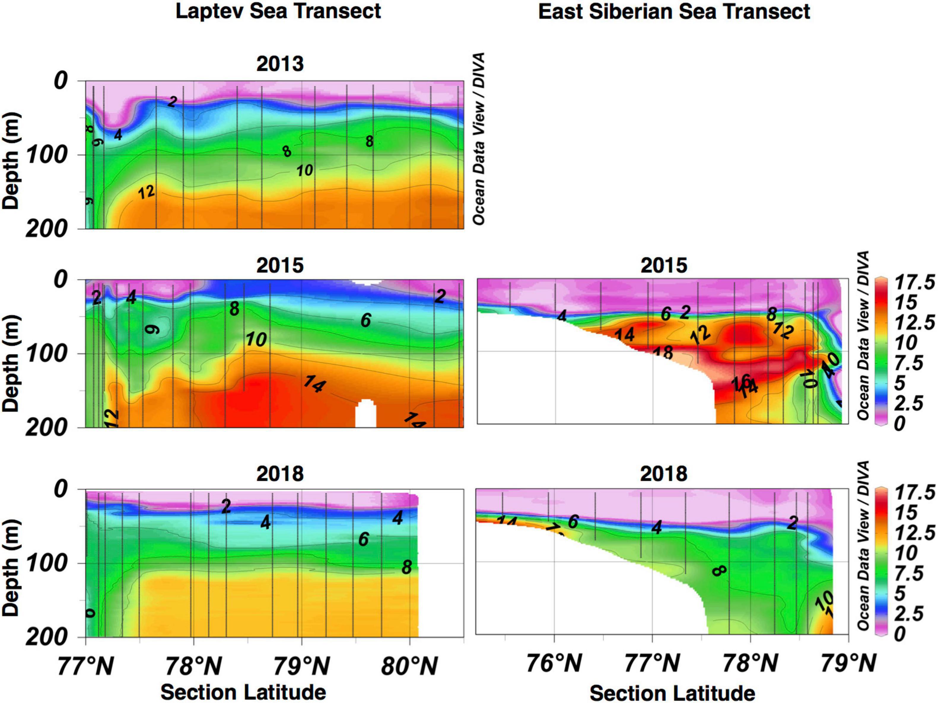
Figure 7. Cross-slope (south-north) distributions of nitrate in the top 0–200 m of the water column for the Laptev Sea (left panels) and East Siberian Sea (right panels) transects during each cruise year. Note the East Siberian Sea transect was not occupied in 2013. The colorbars are identical for all panels, ranging from 0 to 18 mmol m^–3. Contours intervals (2 mmol m^–3) are also identical for all panels. Plots were created using Ocean Data View software, version 4.6.3 (Schlitzer, 2006). The data are displayed using DIVA gridding with automatic length scales enabled.

One might expect a shallower nitracline to be associated with higher NCP; however, such shoaling effectively decreases the depth of the integration in the A and E methods, resulting in a reduction in the calculated NCP. For the case of method D, both the integration depth (50 m) and pre-bloom nitrate concentration (5 mmol m^–3) are prescribed; thus, a shoaling nitracline would introduce higher concentrations into the 0–50 m water column and lower the NCP by “artificially inflating” the summer nitrate inventory. On the other hand, method B is somewhat independent from the nitracline shoaling as the integration depth and pre-bloom concentration are determined by the position of the potential temperature minimum. Similarly, method G is less affected as the integration depth (and pre-bloom nitrate concentration) is determined by a method meant to track the depth of the nitracline.

Consequently, methods A, D, and E potentially underestimated the NCP as a result of a shoaling nitracline, compared to methods B and G. Therefore, selecting a constant depth or nitrate concentration horizon, while suitable for a mean atlas of NCP over large spatial and/or temporal scales (Codispoti et al., 2013), is not optimal when assessing interannual variations in NCP over small areas.

Finally, in the ESS, the integration depths did not vary much among methods or between cruise years, but the nitrate distribution over this transect was very different between 2015 and 2018 (Figure 7, right panels). In 2015, high-nitrate, bottom waters from the shallow shelf were advected offshore and into the Arctic halocline roughly along the 165°E transect line. In contrast, no such high-nutrient waters were advected from the shelf during the 2018 cruise. The intrusion of these shelf waters resulted in somewhat higher pre-bloom concentrations determined for method G whereas those for methods A, D, and E remained constant (winter mixed layer depths were indeterminable along this transect in 2015). The absence of these high-nutrient waters in 2018 led to a decline in NCP between 2015 and 2018 according to method G whereas there was little change in NCP determined by methods A, D, and E. Can we independently verify whether NCP was higher in the ESS in 2015 (compared to 2018)?

This question was addressed using satellite ocean color imagery to determine whether chlorophyll concentrations were higher during summer months in 2015 compared to 2013 and/or 2018. Although such imagery only provides information on the surface skin of the ocean (ignoring NCP at depth), does not capture under-ice production, and is not strictly comparable to NCP as it lacks information detailing community respiration, it does provide a semi-quantitative snapshot of primary production in the NABOS study region. We therefore downloaded MODIS Aqua monthly mapped chlorophyll a concentration data at 4 km resolution¹ and compared available data over two areas that roughly corresponded to the NABOS stations in the ESS (75–83°N, 160–180°E) and Laptev Sea (75–83°N, 110–140°E). Boxplots showing the distributions of the data are shown in Figure 8. Note that no measurements were available from the ESS in July 2013, July 2018, or September 2018 due to sea ice cover. In the ESS, the median chlorophyll a concentrations were highest in 2015 (particularly during July) compared to the available data in 2013 and 2018, supporting the hypothesis that NCP along this transect was higher in 2015. In the Laptev Sea, there were a number of very high (>10 mg m^–3) data points, but median chlorophyll concentrations were generally low and comparable among all the months and years examined, with the exception of September 2015 (very high chlorophyll concentrations). The satellite data therefore support the hypothesis that the apparent drop in NCP observed in 2015 using methods D and E was not representative of true conditions and likely resulted from a bias.

FIGURE 8

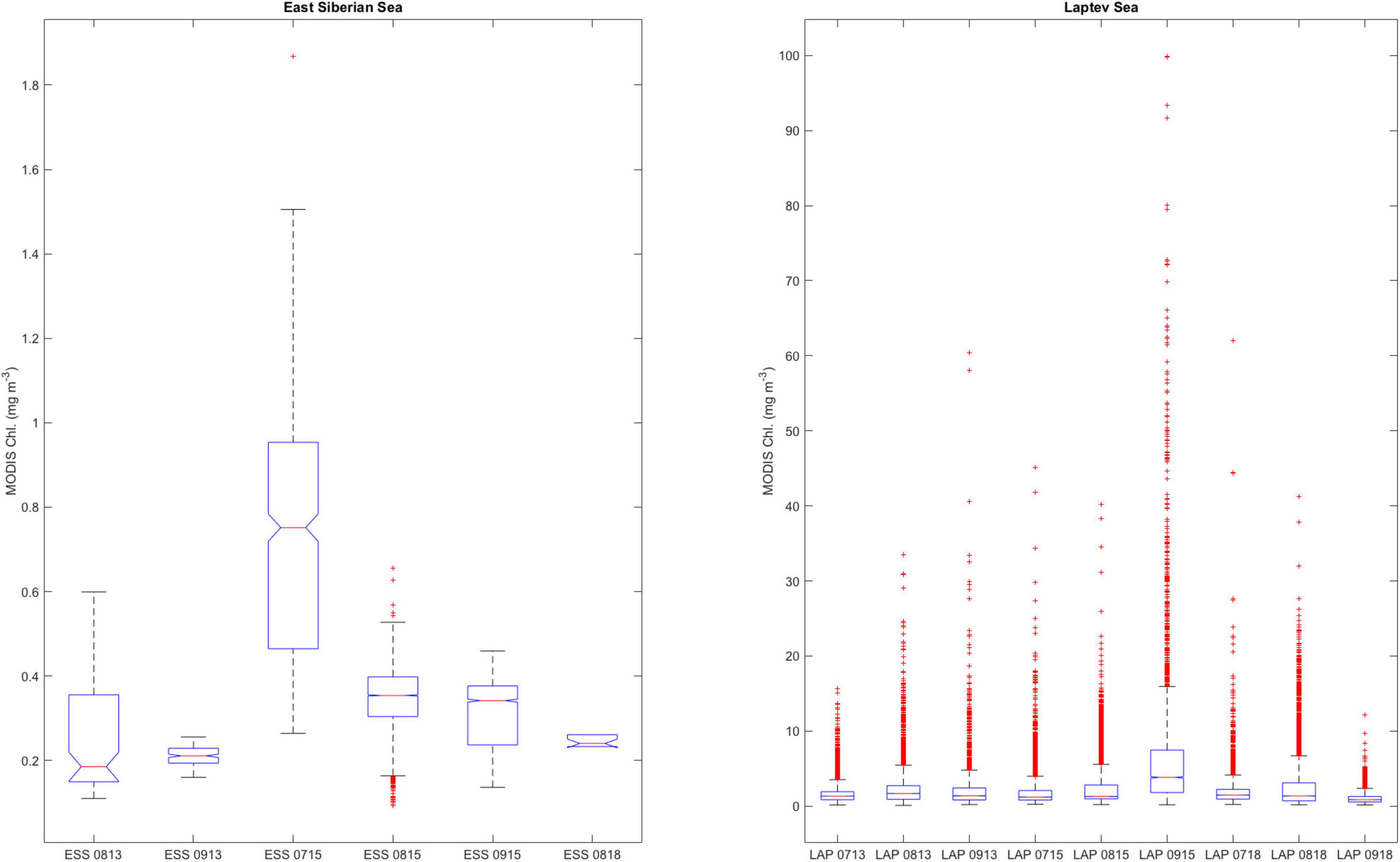
Figure 8. Boxplots of MODIS chlorophyll concentrations (mg m^–3) for two areas defined to represent the East Siberian Sea (left panel), defined as the area enclosed by latitude and longitude ranges of 75–83°N and 160–180°E, respectively, and the Laptev Sea (75–83°N, 110–140°E; right panel). The red line within each box represents the group median, the edges of each box represent the 25th and 75th percentiles, whiskers illustrate the extreme values considered not to be outliers, and the red pluses show outliers. Group medians are expected to be significantly different if the “notches” in the boxes do not overlap. Labels on x-axes indicate the month and year of MODIS observations (e.g., ESS 0813 indicates the East Siberian Sea area during August 2013). Note the different scales of the y-axes for the two panels.

Summary and Conclusion

Warming and loss of sea ice both increase the exposure of the surface ocean to solar radiation and increase stratification. These two physical drivers will have competing impacts on NCP in the Arctic as they decrease light limitation but may increase nutrient limitation on photosynthesis. Reliable estimates of NCP are needed to adequately assess these impacts. However, few data are available to accurately compute NCP. The NABOS study collected requisite measurements in a region particularly lacking in data during late summer 2013, 2015, and 2018.

Winter observations are very sparse on the Siberian slope, inhibiting the calculation of NCP. This requires the need to estimate integration depth and pre-bloom nitrate concentration from summer data. Five methods (A, B, D, E, and G) of estimating the NCP were tested, with different assignments for the pre-bloom nitrate concentration and integration depth. One of these methods (D) assigned a constant pre-bloom nitrate and integration depth for all stations. Two of these methods assigned pre-bloom nitrate concentrations of 5 mmol m^–3 (E) and 6 mmol m^–3 (A), but the integration depth varied among stations. Two more of these methods (B and G) allowed both the pre-bloom nitrate concentration and integration depth to vary among stations.

The mean NCP estimates from all five methods generally agreed with independent studies using similar methods in nearby or overlapping regions. However, significant differences were encountered among the methods when comparing NCP estimates along longitudinal transects occupied in 2013, 2015, and 2018. In the Laptev Sea, a shoaling of the nitracline in 2015 (compared to 2013 and 2018) presented an apparent low bias in NCP estimated using methods with prescribed pre-bloom nitrate and/or integration depths (A, D, and E) whereas no such bias was present in those methods (B and G) that allowed both parameters to vary. In the ESS, the offshore advection of high-nutrient shelf waters in 2015 drastically altered the nitrate distribution compared to conditions in 2018; however, this dynamic shift in hydrographic conditions did not impact NCP estimates using methods with prescribed pre-bloom nitrate and/or integration depths (A, D, and E). In contrast, NCP estimates from method G indicated a 50% difference in NCP between 2015 and 2018. Therefore, assuming a single integration depth of 50 m and a constant pre-bloom nitrate concentration of 5 or 6 mmol m^–3 may underestimate interannual variations in NCP where dynamic, hydrographic changes (e.g., water mass intrusions, meandering fronts, and eddies) occur.

We have also shown that the NCP calculation is very sensitive to the steepness of the nitracline. In regions with particularly sharp nitraclines, a small difference in the integration depth estimate can result in a much larger change in the pre-bloom nitrate assignment and by extension, NCP. Inherent uncertainties in the estimation of integration depths combined with generally coarse vertical resolution of nitrate profile measurements can result in artificially high variability in NCP estimates among stations as well as the potential for high biases. Regional (or section) averages can be used to help reduce such uncertainty and still provide useful data to evaluate spatial and temporal variations in NCP.

Finally, we have introduced a novel method (G) for determining the integration depth and pre-bloom nitrate concentration using measurements of temperature, salinity, nitrate, and oxygen profiles during summer. Although the determination of winter mixed layer depths (method B) remains a preferable method, reliable estimates are sometimes elusive in some areas, particularly over the ESS shelf and slope. It is therefore useful to have a reliable, alternate method for estimating NCP. Additional, alternate methods should continue to be explored; however, the NCP estimates using method G showed promise as sectional means generally agreed with those from method B in most cases. The estimates using method G were also not negatively influenced by the nitracline shoaling observed in the Laptev Sea in 2015 and indicated significant differences in the NCP over the ESS when hydrographic conditions shifted.

Data Availability Statement

The datasets presented in this study can be found in online repositories. The names of the repository/repositories and accession number(s) can be found below: https://arcticdata.io/catalog/view/doi:10.18739/A24X54G9W, https://arcticdata.io/catalog/view/doi%3A10.18739%2FA2FX73Z1F, https://arcticdata.io/catalog/view/doi%3A10.18739%2FA2MS3K255, and https://arcticdata.io/catalog/view/doi%3A10.18739%2FA2RF5KG53.

Author Contributions

MA completed field work associated with this work, wrote the manuscript, and prepared the figures. IP served as the principle investigator of the project that supported this work, evaluated results, edited the manuscript, and provided valuable comments and suggestions that helped to improve the manuscript. RM edited the manuscript and provided valuable comments and suggestions to improve the manuscript. All authors contributed to the article and approved the submitted version.

Funding

MA acknowledges funding from the United States National Science Foundation (PLR-1203146 AM003) and the National Oceanic and Atmospheric Administration (NA15OAR4310156). IP acknowledges funding from the United States National Science Foundation (AON-1203473, AON-1724523, AON-1947162, and 1708427).

Author Disclaimer

Any opinions, findings, and conclusions or recommendations expressed in this material are those of the author(s) and do not necessarily reflect the views of the National Science Foundation or the National Oceanic and Atmospheric Administration.

Conflict of Interest

The authors declare that the research was conducted in the absence of any commercial or financial relationships that could be construed as a potential conflict of interest.

The reviewer TW declared a shared affiliation, though no other collaboration, with one of the authors IP to the handling editor.

Publisher’s Note

All claims expressed in this article are solely those of the authors and do not necessarily represent those of their affiliated organizations, or those of the publisher, the editors and the reviewers. Any product that may be evaluated in this article, or claim that may be made by its manufacturer, is not guaranteed or endorsed by the publisher.

Supplementary Material

The Supplementary Material for this article can be found online at: https://www.frontiersin.org/articles/10.3389/fmars.2022.812912/full#supplementary-material

Footnotes

1. ^ https://oceandata.sci.gsfc.nasa.gov/directaccess/MODIS-Aqua/Mapped/Monthly/4km/

References

Alkire, M. (2019). Ocean Conductivity, Temperature, Density (CTD), Oxygen, and Nitrate Profiles, Eurasian and Makarov basins, Arctic Ocean, 2013-2018. Santa Barbara, CA: Arctic Data Center, doi: 10.18739/A24X54G9W

CrossRef Full Text | Google Scholar

Alkire, M., and Rember, R. (2019). Geochemical Observations of Seawater in the Eastern Eurasian Basin, Arctic Ocean, 2018. Santa Barbara, CA: Arctic Data Center, doi: 10.18739/A2FX73Z1F

CrossRef Full Text | Google Scholar

Alkire, M. B., Falkner, K. K., Morison, J., Collier, R. W., Guay, C. K., Desiderio, R. A., et al. (2010). Sensor-based profiles of the NO parameter in the central Arctic and southern Canada Basin: new insights regarding the cold halocline. Deep Sea Res. I 57, 1432–1443.

Google Scholar

Alkire, M. B., Morison, J., and Andersen, R. (2015). Variability in the meteoric water, sea-ice melt, and Pacific water contributions to the central Arctic Ocean, 2000-2014. J. Geophys. Res. 120, 1573–1598. doi: 10.1002/2014JC010023

CrossRef Full Text | Google Scholar

Alkire, M. B., Rember, R., and Polyakov, I. (2019). Discrepancy in the identification of the Atlantic/Pacific front in the central Arctic Ocean: NO versus nutrient relationships. Geophys. Res. Lett. 46, 3843–3852. doi: 10.1029/2018GL081837

CrossRef Full Text | Google Scholar

Anderson, L. G., Andersson, P. S., Bjork, G., Jones, E. P., Jutterstrom, S., and Wahlstrom, I. (2013). Source and formation of the upper halocline of the Arctic Ocean. J. Geophys. Res. 118, 410–421. doi: 10.1029/2012JC008291

CrossRef Full Text | Google Scholar

Anderson, L. G., Bjork, G., Jutterstrom, S., Pipko, I., Shakhova, N., Semiletov, I., et al. (2011). East Siberian Sea, an arctic region of very high biogeochemical activity. Biogeosci. Discuss. 8, 1137–1167.

Google Scholar

Anderson, L. G., Jones, E. P., and Swift, J. H. (2003). Export production in the central Arctic Ocean evaluated from phosphate deficits. J. Geophys. Res. 108:3199. doi: 10.1029/2001JC001057

CrossRef Full Text | Google Scholar

Ardyna, M., Babin, M., Gosselin, M., Devred, E., Rainville, L., and Tremblay, J. -É (2014). Recent Arctic Ocean sea ice loss triggers novel fall phytoplankton blooms. Geophys. Res. Lett. 41, 6207–6212. doi: 10.1002/2014GL061047

CrossRef Full Text | Google Scholar

Arrigo, K. R., Perovich, D. K., Pickart, R. S., Brown, Z. W., van Dijken, G. L., Lowry, K. E., et al. (2012). Massive phytoplankton blooms under Arctic sea ice. Science 336:1408. doi: 10.1126/science.1215065

PubMed Abstract | CrossRef Full Text | Google Scholar

Arrigo, K. R., van Dijken, G., and Pabi, S. (2008). Impact of a shrinking Arctic ice cover on marine primary production. Geophys. Res. Lett. 35:L19603. doi: 10.1029/2008GL035028

CrossRef Full Text | Google Scholar

Bates, N. R., and Mathis, J. T. (2009). The Arctic Ocean marine carbon cycle: evaluation of air-sea CO2 exchanges, ocean acidification impacts and potential feedbacks. Biogeosci. Discuss. 6, 2433–2459.

Google Scholar

Bauch, D., Dmitrenko, I. A., Wegner, C. Hölemann, J., Kirillov, S. A., Timokhov, L. A., et al. (2009). Exchange of laptev sea and arctic ocean halocline waters in response to atmospheric forcing. J. Geophys. Res. 114:C05008. doi: 10.1029/2008JC005062

CrossRef Full Text | Google Scholar

Broecker, W. S. (1974). “NO”: a conservative water mass tracer. Earth Planet. Sci. Lett. 23, 100–107.

Google Scholar

Burgers, T. M., Tremblay, J.-E., Else, B. G. T., and Papakyriakou, T. N. (2020). Estimates of net community production from multiple approaches surrounding the spring ice-edge bloom in Baffin Bay. Elem Sci. Anth. 8:013. doi: 10.1525/elementa.013

CrossRef Full Text | Google Scholar

Cai, W. J., Chen, L., Chen, B., Gao, Z., Lee, S. H., Chen, J., et al. (2010). Decrease in the CO2 uptake capacity in an ice-free Arctic Ocean Basin. Science 329, 556–559. doi: 10.1126/science.1189338

PubMed Abstract | CrossRef Full Text | Google Scholar

Carmack, E., Barber, D., Christensen, J., Macdonald, R., Rudels, B., and Sakshaug, E. (2006). Climate variability and physical forcing of the food webs and the carbon budget on panarctic shelves. Progr. Oceanogr. 71, 145–181. doi: 10.1016/j.pocean.2006.10.005

CrossRef Full Text | Google Scholar

Carmack, E., and Wassmann, P. (2006). Food webs and physical-biological coupling on pan-Arctic shelves: unifying concepts and comprehensive perspectives. Progr. Oceanogr. 71, 446–477. doi: 10.1016/j.pocean.2006.10.004

CrossRef Full Text | Google Scholar

Codispoti, L. A., Kelly, V., Thessen, A., Matrai, P., Suttles, S., Hill, V., et al. (2013). Synthesis of primary production in the Arctic Ocean: III. Nitrate and phosphate based estimates of net community production. Progr. Oceanogr. 110, 126–150. doi: 10.1016/j.pocean.2012.11.006

CrossRef Full Text | Google Scholar

Else, B. G. T., Galley, R. J., Lansard, B., Barber, D. G., Brown, K., Miller, L. A., et al. (2013). Further observations of a decreasing atmospheric CO2 uptake capacity in the Canada Basin (Arctic Ocean) due to sea ice loss. Geophys. Res. Lett. 40, 1132–1137. doi: 10.1002/grl.50268

CrossRef Full Text | Google Scholar

Falkowski, P., Laws, E., Barber, R., and Murray, J. (2003). “Phytoplankton and their role in primary, new, and export production,” in Ocean Biogeochemistry, ed. M. R. Fasham (Berlin: Springer), 99–121. doi: 10.1007/978-3-642-55844-3_5

CrossRef Full Text | Google Scholar

Holmes, R. M., McClelland, J. W., Peterson, B. J., Tank, S. E., Bulygina, E., Eglinton, T. I., et al. (2012). Seasonal and annual fluxes of nutrients and organic matter from large rivers to the Arctic Ocean and surrounding seas. Estuar. Coast. 35, 369–382. doi: 10.1007/s12237-011-9386-6

CrossRef Full Text | Google Scholar

Macdonald, R. W., Kuzyk, Z. A., and Johannessen, S. C. (2015). It is not just about the ice: a geochemical perspective on the changing Arctic Ocean. J. Environ. Stud. Sci. 5, 288–301. doi: 10.1007/s13412-015-0302-4

CrossRef Full Text | Google Scholar

Macdonald, R. W., Wong, C. S., and Erickson, P. E. (1987). Distribution of nutrients in the southeastern Beaufort Sea: implications for water circulation and primary production. J. Geophys. Res. 92, 2939–2952. doi: 10.1029/jc092ic03p02939

CrossRef Full Text | Google Scholar

McClelland, J. W., Holmes, R. M., Dunton, K. H., and Macdonald, R. W. (2012). The arctic ocean estuary. Estuar. Coast. 35, 353–368. doi: 10.1007/s12237-010-9357-3

CrossRef Full Text | Google Scholar

McClelland, J. W., Townsend-Small, A., Holmes, R. M., Pan, F., Stieglitz, M., Khosh, M., et al. (2014). River export of nutrients and organic matter from the North Slope of Alaska to the Beaufort Sea. Water Resour. Res. 50, 1823–1839. doi: 10.1002/2013WR014722

CrossRef Full Text | Google Scholar

McLaughlin, F. A., and Carmack, E. C. (2010). Deepening of the nutricline and chlorophyll maximum in the Canada Basin interior, 2003-2009. Geophys. Res. Lett. 37:L24602. doi: 10.1029/2010GL045459

CrossRef Full Text | Google Scholar

Nishino, S., Itoh, M., Williams, W. J., and Semiletov, I. (2013). Shoaling of the nutricline with an increase in near-freezing temperature water in the Makarov Basin. J. Geophys. Res 118, 635–649. doi: 10.1029/2012JC008234

CrossRef Full Text | Google Scholar

Nishino, S., Shimada, K., Itoh, M., Yamamoto-Kawai, M., and Chiba, S. (2008). East-west differences in water mass, nutrient, and chlorophyll a distributions in the sea ice reduction region of the western Arctic Ocean. J. Geophys. Res. 113:C00A01. doi: 10.1029/2007JC004666

CrossRef Full Text | Google Scholar

Pickart, R. S., Spall, M. A., and Mathis, J. T. (2013). Dynamics of upwelling in the Alaskan Beaufort Sea and associated shelf–basin fluxes. Deep Sea Res. Part 1 76, 35–51. doi: 10.1016/j.dsr.2013.01.007

CrossRef Full Text | Google Scholar

Polyakov, I. (2016a). NABOS - Chemistry Data 2013. Santa Barbara, CA: Arctic Data Center, doi: 10.18739/A2M03XX62

CrossRef Full Text | Google Scholar

Polyakov, I. (2016b). NABOS II - Chemistry Data 2015. Santa Barbara, CA: Arctic Data Center, doi: 10.18739/A2VM42X8F

CrossRef Full Text | Google Scholar

Polyakov, I. V., Rippeth, T. P., Fer, I., Baumann, T. M., Carmack, E. C., Ivanov, V. V., et al. (2020a). Intensification of near-surface currents and shear in the Eastern Arctic Ocean. Geophys. Res. Lett. 46:e2020GL089469. doi: 10.1029/2020GL089469

CrossRef Full Text | Google Scholar

Polyakov, I. V., Rippeth, T., Fer, I., Alkire, M., Baumann, T., Carmack, E., et al. (2020b). Weakening of cold halocline layer exposes sea ice to oceanic heat in the eastern Arctic Ocean. J. Clim. 33, 1–43. doi: 10.1175/JCLI-D-19-0976.1

CrossRef Full Text | Google Scholar

Popova, E. E., Yool, A., Coward, A. C., Aksenov, Y. K., Alderson, S. G., de Cuevas, B. A., et al. (2010). Control of primary production in the Arctic by nutrients and light: insights from a high resolution ocean general circulation model. Biogeosciences 7, 3569–3591. doi: 10.5194/bg-7-3569-2010

CrossRef Full Text | Google Scholar

Rainville, L., and Woodgate, R. A. (2009). Observations of internal wave generation in the seasonally ice-free Arctic. Geophys. Res. Lett. 36:L23604. doi: 10.1029/2009GL041291

CrossRef Full Text | Google Scholar

Rudels, B., Anderson, L. G., and Jones, E. P. (1996). Formation and evolution of the surface mixed layer and halocline of the Arctic Ocean. J. Geophys. Res. 101, 8807–8821. doi: 10.1029/96JC00143

CrossRef Full Text | Google Scholar

Rudels, B., Jones, P., Schauer, U., and Eriksson, P. (2004). Atlantic sources of the Arctic Ocean surface and halocline waters. Polar Res. 23, 181–208. doi: 10.111/j.1751-8369.2004.tb00007.x

CrossRef Full Text | Google Scholar

Sakamoto, C. M., Johnson, K. S., and Coletti, L. J. (2009). Improved algorithm for the computation of nitrate concentrations in seawater using an in situ ultraviolet spectrophotometer. Limnol. Oceanogr. Methods 7, 132–143. doi: 10.4319/lom.2009.7.132

CrossRef Full Text | Google Scholar

Sakshaug, E. (2004). “Primary and secondary production in the Arctic Seas,” in The Organic Carbon Cycle in the Arctic Ocean, eds R. Stein and R. MacDonald (Berlin: Springer), 57–81. doi: 10.1007/978-3-642-18912-8_3

CrossRef Full Text | Google Scholar

Schlitzer, R. (2006). Ocean Data View. Avaliable online at: http://odv.awi.de.

Google Scholar

Semiletov, I., Dudarev, O., Luchin, V., Charkin, A., Shin, K.-H., and Tanaka, N. (2005). The East Siberian Sea as a transition zone between Pacific-derived waters and Arctic shelf waters. Geophys. Res. Lett. 32:L10614. doi: 10.1029/GL022490

CrossRef Full Text | Google Scholar

Slagstad, D., Wassmann, P. F. J., and Ellingsen, I. (2015). Physical constrains and productivity in the future Arctic Ocean. Front. Mar. Sci. 2:85. doi: 10.3389/fmars.2015.00085

CrossRef Full Text | Google Scholar

Steele, M., and Boyd, T. (1998). Retreat of the cold halocline layer in the Arctic Ocean. J. Geophys. Res. 103, 10419–10435. doi: 10.1029/98JC00580

CrossRef Full Text | Google Scholar

Uflsbo, A., Cassar, N., Korhonen, M., van Heuven, S., Hoppema, M., Kattner, G., et al. (2014). Late summer net community production in the central Arctic Ocean using multiple approaches. Glob. Biogeochem. Cycles 28, 1129–1148. doi: 10.1002/2014GB004833

CrossRef Full Text | Google Scholar

Vancoppenolle, M., Bopp, L., Madec, G., Dunne, J., Ilyina, T., Halloran, P. R., et al. (2013). Future Arctic Ocean primary productivity from CMIP5 simulations: uncertain outcome, but consistent mechanisms. Glob. Biogeochem. Cycles 27, 605–619. doi: 10.1002/gbc.20055

CrossRef Full Text | Google Scholar