Transport Structure of the South Atlantic Ocean Derived From a High-Resolution Numerical Model and Observations

Xu, Xiaobiao; Chassignet, Eric P.; Dong, Shenfu; Baringer, Molly O.

doi:10.3389/fmars.2022.811398

ORIGINAL RESEARCH article

Front. Mar. Sci., 01 March 2022

Sec. Physical Oceanography

Volume 9 - 2022 | https://doi.org/10.3389/fmars.2022.811398

This article is part of the Research Topic The Role of the South Atlantic on the Interbasin and Pole-to-Pole Connections View all 11 articles

Transport Structure of the South Atlantic Ocean Derived From a High-Resolution Numerical Model and Observations

$\r\nXiaobiao Xu*$ Xiaobiao Xu^1*

Eric P. Chassignet¹

Shenfu Dong² $Molly O. Baringer\r\n$ Molly O. Baringer²

¹Center for Ocean-Atmospheric Prediction Studies (COAPS), Florida State University, Tallahassee, FL, United States
²Atlantic Oceanographic and Meteorological Laboratory (AOML), National Oceanic and Atmospheric Administration, Miami, FL, United States

The South Atlantic Ocean plays an important role in the Atlantic meridional overturning circulation (AMOC), connecting it to the Indian and Pacific Oceans as part of the global overturning circulation system. Yet, there are still open questions regarding the relative importance of the warm water versus cold water sources in the upper limb of the AMOC and on the detailed circulation pathways of the North Atlantic Deep Water (NADW) in the lower limb. These questions are addressed using model outputs from a 60-year, eddying global ocean-sea ice simulation that are validated against observations. We find that the Pacific Antarctic Intermediate Water (AAIW) plays a role in setting the temperature and salinity properties of the water in the subtropical South Atlantic, but that the upper limb of the AMOC originates primarily from the warm Indian water through the Agulhas leakage (9.8 Sv of surface water + 3.5 of AAIW) and that only a relatively small contribution of 1.5 Sv colder, fresher AAIW originates from the Pacific Ocean. In the lower limb, the NADW flows southward as a deep western boundary current all the way to 45°S and then turns eastward to flow across the Mid-Atlantic Ridge near 42°S before leaving the Atlantic Ocean, although there is clockwise recirculation in the Brazil, Angola, and Cape Basins.

Introduction

In the Atlantic Ocean, warm water from the South Atlantic flows northward in approximately the upper 1000 m, loses buoyancy to the atmosphere by cooling en route to the northern North Atlantic, and eventually sinks and returns southward at depth as the cold North Atlantic Deep Water (NADW). The temperature difference between the upper and lower limbs of this Atlantic meridional overturning circulation (AMOC) leads to a large northward oceanic heat transport throughout the entire Atlantic basin, in contrast to the poleward (northward and southward from the equator) heat transport in the Pacific and Indian Oceans (e.g., Macdonald and Baringer, 2013). The South Atlantic Ocean, defined here as the area south of 20°S (Figure 1), plays an important role in that it is through this region where the upper and lower AMOC limbs are connected to the Indian and Pacific Oceans and are entangled in the global overturning circulation system (e.g., Gordon, 1986; Broeker, 1991; Schmitz, 1995, 1996; Richardson, 2008; Talley, 2013). Thus, a comprehensive knowledge of the circulation in this region is essential to our understanding of the spatial structure and temporal variability of the AMOC.

FIGURE 1

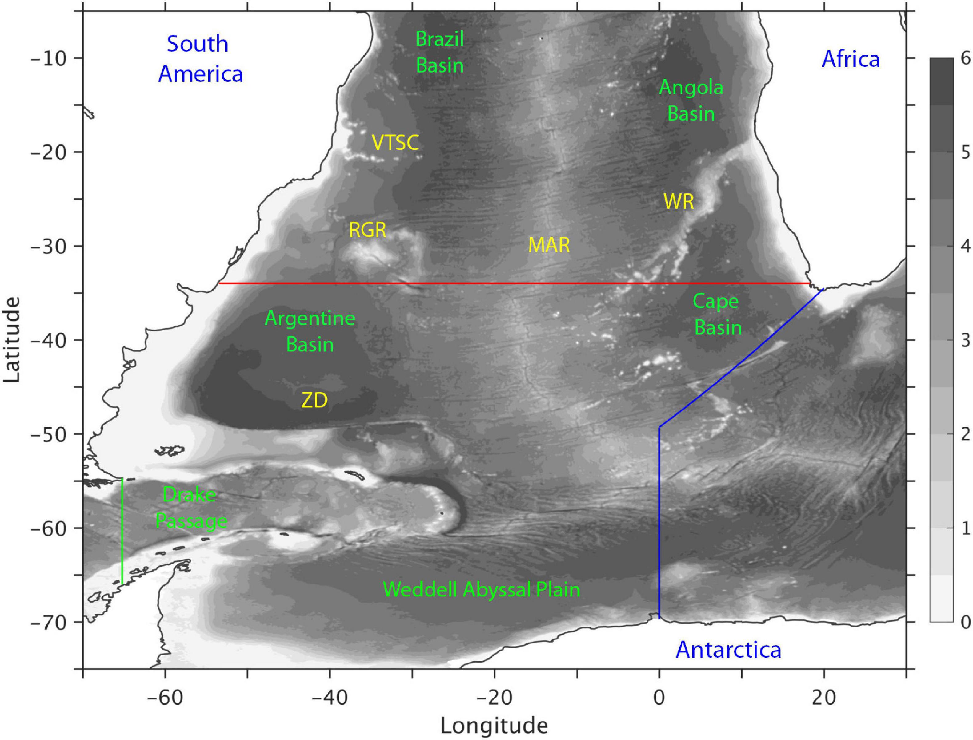
Figure 1. Model bathymetry (in km) along with key topographic features in the South Atlantic Ocean: Vitoria-Trindade Seamount Chain (VTSC), Rio-Grande Rise (RGR), Mid-Atlantic Ridge (MAR), Walvis Ridge (WR), Zapiola Drift (ZD). Red, green, and blue lines denote three sections where significant observations have been obtained and the observations are used to evaluate the model results: 34°S in the South Atlantic, 65°W in Drake Passage, and the Prime Meridian-Good Hope (PM-GH) transect southwest of Africa.

Significant observations have been made in the last 15 years or so toward quantifying and monitoring the AMOC in the South Atlantic, particularly along a latitude near 34.5°S (e.g., Baringer and Garzoli, 2007; Dong et al., 2009, 2014, 2015; Garzoli et al., 2013; Meinen et al., 2013, 2018; Goes et al., 2015). These observations, which consist of moorings, expendable Bathythermograph (XBT), and Argo float measurements, yield a time mean AMOC transport in the range of 14-20 Sv. They also showed that there is significant AMOC variability on several timescales, similar to that observed by the RAPID array at 26.5°N (e.g., Smeed et al., 2018). Beyond 34.5°S, however, the observations in the South Atlantic remain sparse and short (in time). Overall, our understanding of the spatial structure of the time mean circulation is mostly limited to the schematic of Stramma and England (1999) and even less is known about its temporal variability. Numerical studies of the AMOC have primarily dealt with the zonally integrated AMOC transport index and little on the spatial structure of the circulation; see Hirschi et al. (2020) and Roberts et al. (2020) for a recent review of AMOC representation in high-resolution ocean simulations and climate models, respectively. Furthermore, most of these numerical studies focused on the North Atlantic since it is only in the last decade or so that AMOC observations became available in the South Atlantic.

There is the long-standing debate (Gordon, 2001) regarding as to whether the upper limb of the AMOC in the South Atlantic originates from the warm, saline Indian waters through the southern rim of Africa (e.g., Gordon, 1986; Saunders and King, 1995) or from the cooler, fresher Pacific water through the Drake Passage (e.g., Rintoul, 1991; Schlitzer, 1996). Although recent studies seem to favor the warm-water route from the Indian Ocean through the Agulhas leakage (e.g., Richardson, 2007; Beal et al., 2011), the relative contributions of cold versus warm water are still uncertain (Garzoli and Matano, 2011; Bower et al., 2019). For example, Rodrigues et al. (2010) estimated a cold-water contribution of 4.7 Sv based on quasi-isobaric subsurface floats and hydrographic data. This value is close to the estimate of Rühs et al. (2019) derived from an eddy-rich model, but it is significantly higher than several other estimates of 1-2 Sv based on numerical simulations and/or reanalysis (e.g., Speich et al., 2001; Donners and Drijfhout, 2004; Friocourt et al., 2005; Rousselet et al., 2020). Furthermore, most of these estimates were computed from Lagrangian analyses and the question then arises as to how these results would compare to a volume transport structure and/or water properties estimated from a Eulerian perspective. At depth, in the lower limb of the AMOC, many of the details of the circulation are still unknown, such as the exact location/latitude where the NADW in the Deep Western Boundary Current (DWBC) turns eastward and flows across the Mid-Atlantic Ridge (MAR). In recent decades, much attention has been paid to an eastward flow of the NADW near 22°S (e.g., Speer et al., 1995; Stramma and England, 1999; Arhan et al., 2003; Hogg and Thurnherr, 2005; van Sebille et al., 2012; Garzoli et al., 2015). However, both the magnitude of this flow and the extent of the eastward penetration in the Angola Basin are still debated.

Three-dimensional circulation information beyond the existing observations is required in order to address the above questions. In this paper, these questions are addressed by performing a detailed Eulerian and Lagrangian analysis of the three-dimensional circulation of a high-resolution numerical model validated against observations. We find that the Pacific AAIW plays a role in setting the temperature and salinity properties of the water in the subtropical South Atlantic, but that the upper limb of the AMOC originates primarily from the warm Indian water through the Agulhas leakage (9.8 Sv of surface water + 3.5 Sv of AAIW) and that only a relatively small contribution of 1.5 Sv colder, fresher AAIW originates from the Pacific Ocean. In the lower limb, the NADW flows southward as a deep western boundary current all the way to 45°S and then turns eastward to flow across the Mid-Atlantic Ridge near 42°S before leaving the Atlantic Ocean, although there is clockwise recirculation in the Brazil, Angola, and Cape Basins.

The paper is structured as follows. In Section “Numerical Simulation and Validation,” we first summarize the configuration and basic features of the numerical simulation. Before the model can be used to increase our understanding of the circulation on the South Atlantic, the model results must be in reasonable agreement with the existing observations. The bulk of Section “Numerical Simulation and Validation” therefore compares in detail the modeled large-scale circulation pattern and the transport structure to observations. The validated model results are then used to document the time mean circulation pattern in the South Atlantic (Section “Circulation pathways in the South Atlantic Ocean”). Summary and discussions follow in Section “Summary and Discussion”.

Numerical Simulation and Validation

The numerical results presented in this study are from a long-term global ocean-sea ice hindcast simulation performed using the Hybrid Coordinate Ocean Model (HYCOM, Bleck, 2002; Chassignet et al., 2003), coupled with the Community Ice CodE (CICE, Hunke and Lipscomb, 2008). The vertical coordinate of the HYCOM is isopycnic in the stratified open ocean and makes a dynamically smooth and time-dependent transition to terrain following in the shallow coastal regions and to fixed pressure levels in the surface mixed layer and/or unstratified seas. In doing so, the model combines the advantages of the different coordinate types in simulating coastal and open ocean circulation features simultaneously (e.g., Chassignet et al., 2006).

The simulation has a horizontal resolution of 1/12° (∼6 km in the area of interest) and a vertical resolution of 36 layers (in σ₂). It is initialized using the January temperature and salinity from an ocean climatology (Carnes, 2009), and is forced using the latest surface-atmospheric reanalysis dataset JRA55 (Tsujino et al., 2018), which has a refined grid spacing of ∼55 km and temporal interval of 3 h and covers the period of 1958–2018. The surface heat flux forcing is computed using the shortwave and longwave radiations from JRA55, as well as the latent and sensible heat fluxes derived from the CORE bulk formulae of Large and Yeager (2004) and the model sea surface temperature. The surface freshwater forcing includes evaporation, precipitation, and climatological river runoffs. In addition, the model sea surface salinity is restored toward ocean climatology (Carnes, 2009) with a restoring timescale of two months, and it is constrained by an ad hoc assumption of zero global net flux at each time step. The wind stress is calculated from the atmospheric wind velocity and does not take into account the shear introduced by the ocean currents. The simulation starts from rest and is integrated over 1958–2018 with no data assimilation. The horizontal diffusion parameters are listed in Supplementary Table 1. A detailed evaluation of the modeled global ocean circulation and sea ice is provided in Chassignet et al. (2020). In this study, we focus on the South Atlantic over the last 40 years of the simulation (1979–2018), which are deemed as being representative of the time-mean circulation after spin-up.

In the remainder of this section, we first evaluate the large-scale surface circulation and then quantify the modeled transport structure at three sections in the South Atlantic: 34°S, 65°W in the Drake Passage, and a Prime Meridian-Good Hope section southwest of Africa (Figure 1). Significant observations have been conducted at these locations and they provide a benchmark for evaluating the realism of the modeled transports, which will be used to document the transport structure of the South Atlantic in Section “Circulation pathways in the South Atlantic Ocean.”

Surface Circulation Pattern

Figure 2 compares the observed and modeled mean sea surface height (SSH), SSH variability, and eddy kinetic energy (EKE) of the surface currents in the South Atlantic. The observed mean SSH (Figure 2A) is from the latest mean dynamic topography climatology CNES-CLS18 (Mulet et al., 2021) while the SSH variability (Figure 2C) and surface EKE (Figure 2E) are derived from the AVISO data over 1993–2018, the same time period used for the model results. In the western side of the domain, part of the Antarctic Circumpolar Current (ACC) turns north after passing the Drake Passage and becomes the Malvinas Current (also called the Falkland Current). The latter continues to flow northward along the continental shelf of Argentina until it meets the southward flowing Brazil Current south of the Rio de la Plata estuary near 36°S. The confluence of these two western boundary currents with opposite directions and very different properties (warm salty subtropical water versus cold fresh subantarctic water) leads to numerous high-energy eddies and thus strong variability in this so-called Brazil-Malvinas confluence zone (Figures 2C–F). In the south between 50°W and 20°E, the ACC as a whole is mostly zonal and exhibits tighter mean SSH contours near 40°W south of the Zapiola Drift and near 10°W over the MAR. Overall, there is a good agreement between the model and the observations in the western and southern part of the domain, with the exception of a slightly lower model SSH variability offshore in the Brazil-Malvinas confluence zone near 40°S and, likely related, a weaker signature of the Zapiola gyre in mean SSH.

FIGURE 2

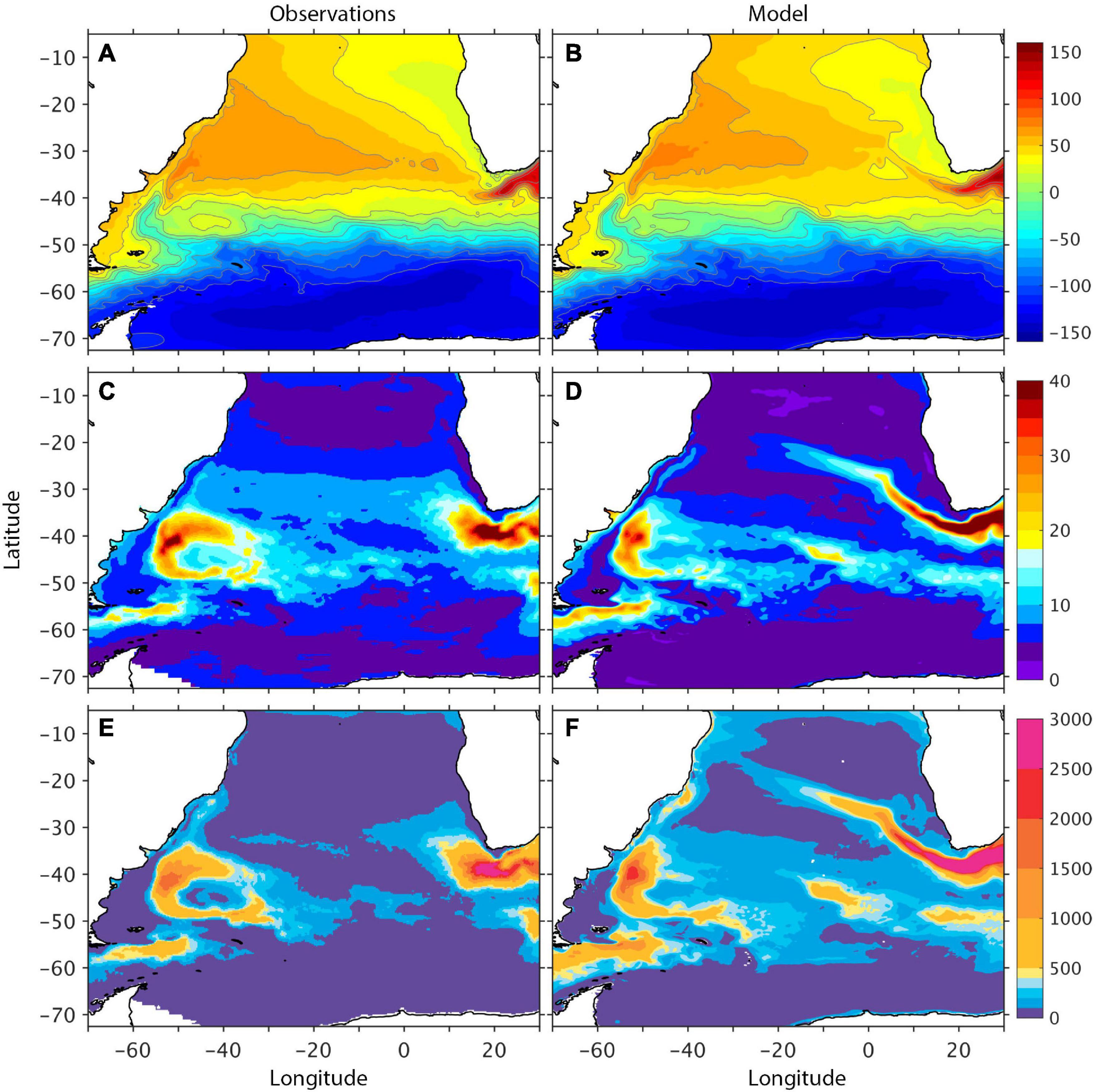
Figure 2. Observed and modeled distributions of (A,B) time mean sea surface height (SSH, in cm), (C,D) SSH standard deviation (in cm), and (E,F) eddy kinetic energy (EKE, in cm² s^–2) of the surface current in the southern Atlantic. In observation, the mean SSH is based on long-term climatology CNES-CLS18 (Mulet et al., 2021); the SSH standard deviation and EKE are based on AVISO data in 1993–2018. All model results are also in 1993–2018.

West of Africa, the model results exhibit a narrow tongue of high SSH variability/EKE that extends further northwest into the South Atlantic than in observations. Plots of the SSH variability for both the model and the observations along the Prime Meridian over the observational period of 1993–2018 in Supplexmentary Figure 1 show that the modeled Agulhas rings are stronger and cross the Prime Meridian within a smaller latitudinal range than in the observations, therefore impacting the regional circulation pattern in the eastern South Atlantic. This is a common feature for many eddying models (e.g., Maltrud and McClean, 2005; Dong et al., 2011; van Sebille et al., 2012), and there is no easy fix short of increasing the horizontal resolution to fully represent the ocean-atmospheric feedback and retain a reasonable level of surface EKE; see Chassignet et al. (2020) and discussion in the summary section.

Water Mass and Transport Across 34°S

Figures 3A–D display a vertical section of the time-mean potential temperature θ and salinity S at 34°S. The observations are based on the gridded monthly Argo profiles (2004–2014) for the upper 2000 m and the World Ocean Atlas 2013 (WOA13, Locarnini et al., 2013; Zweng et al., 2013) below 2000 m (one should note that Argo profiles are sparse in the South Atlantic and that WOA13 data are used in the upper 2000 m when Argo data are missing); the model results are 40-year means from 1979 to 2018. The water column at this latitude can be divided into four density layers of water masses characterized by their salinity (θ decreases monotonically): saline near surface water (σ₂<35.65 kg m^–3), fresh Antarctic Intermediate Water (AAIW, 35.65 < σ₂< 36.58), saline NADW (36.58 < σ₂< 37.12), and fresh Antarctic Bottom Water (AABW, σ₂> 37.12). There is a good agreement in the θ and S distributions, such as the warm/saline anomaly in 2000–3000 m depth range associated with the NADW in the DWBC. For a more quantitative comparison, Figures 3E,F display the volumetric θ-S diagram along 34°S for both observations and model results. The color shading is volume percentage of water mass calculated with a Δθ×ΔS grid resolution of 0.1°C × 0.02 psu, and the circled black/red lines are the volume weighted θ-S values calculated for each of the HYCOM density layers. The AAIW occupies ∼20% of the volume at this latitude in both the observations and model results, and this water mass as a whole is 0.35°C warmer and 0.11 psu saltier in the model than in observations (the maximum θ-S difference is ∼0.8°C and 0.18 psu for an individual density layer). Above the AAIW, the modeled near surface water is about 0.8°C warmer than observations and its salinity is very close to the observations (error on the order of 0.02 psu). Below the AAIW, the differences in θ-S properties are small (0.1°C and 0.02 psu, respectively), but the model results exhibit more AABW and less NADW than in WOA13. The latter is present in the early stage of the simulation and, to a large degree, it reflects the difference between WOA13 and the ocean climatology used for model initialization. Overall, the modeled water properties are consistent with observations – the reader is referred to Chassignet et al. (2020) for a detailed discussion of the temporal evolution of the model’s temperature and salinity.

FIGURE 3

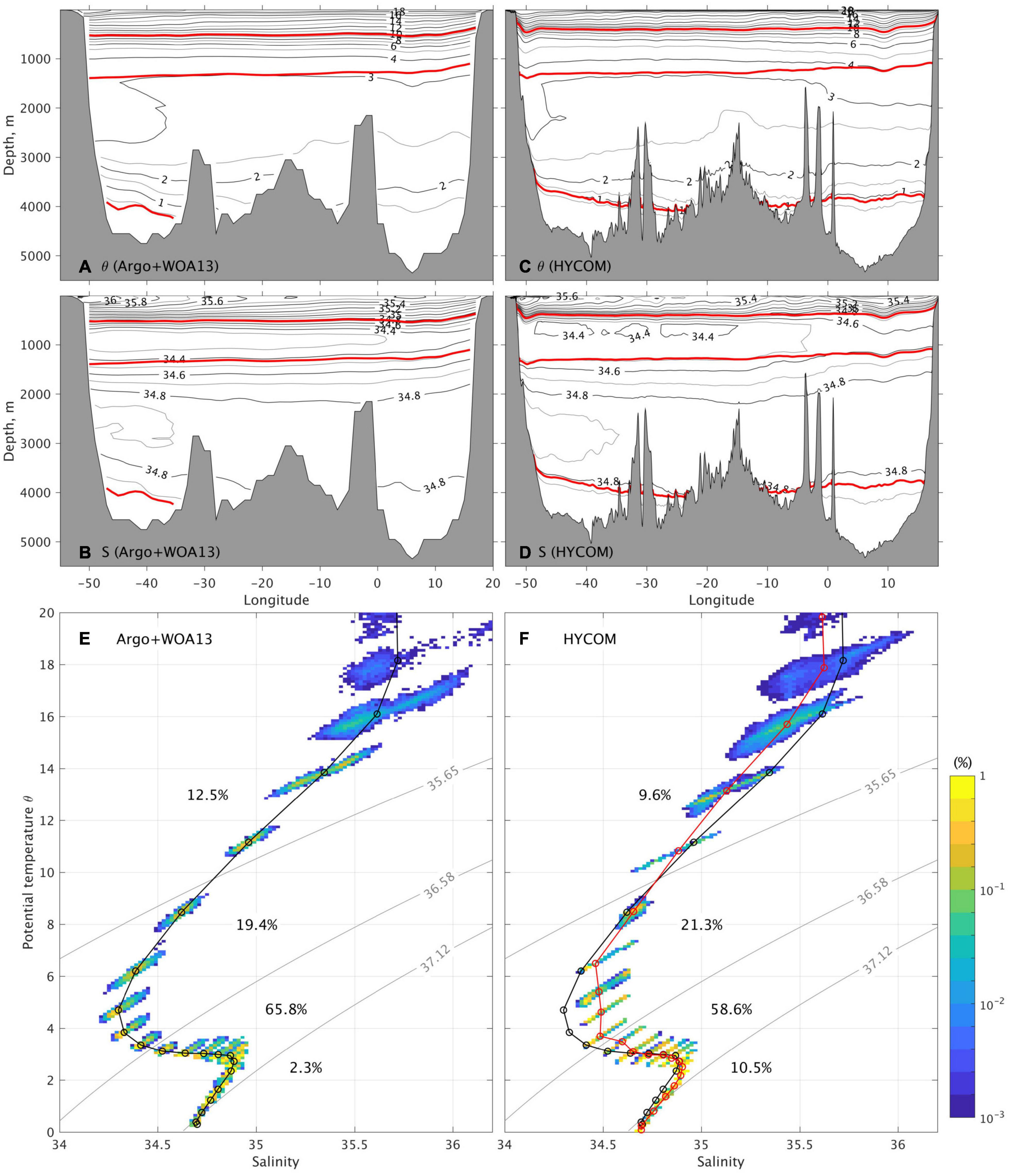
Figure 3. (A–D) Potential temperature θ and salinity S distributions across 34°S. Observations are based on a combination of Argo profiles for the top 2000 m and World Ocean Atlas 2013 (WOA13) below 2000 m; model results are from the global 1/12° HYCOM simulation. Three red lines denote isopycnic surfaces (σ₂ of 35.65, 36.58, and 37.12 kg m^–3) that divide the water column into near surface water, Antarctic Intermediate Water (AAIW), North Atlantic Deep Water (NADW), and Antarctic Bottom Water (AABW). (E,F) Volumetric θ -S diagram along 34°S. Color shading shows the volume percentage for water mass with Δθ, ΔS resolution of 0.1°C, 0.02 psu (percentages for near surface water, AAIW, NADW and AABW are also listed); circled lines are volume-weighted θ -S profile in observations (black) and model results (red).

The time mean meridional velocity across 34°S and the corresponding volume transports for the four water masses defined above are shown in Figure 4. The observations consist of geostrophic transports derived from θ/S profiles (Argo-WOA13 data) and Ekman transports from the wind stress; see Dong et al. (2014) for details. The model results are 40-year means (1979–2018). The main circulation at this latitude consists of the South Atlantic subtropical gyre (southward Brazil Current near the western boundary and northward interior flow) and the AMOC (northward Bengula Current near the eastern boundary and southward DWBC near the western boundary). Quantitatively, the total transport of the southward western boundary current is about 42 Sv (12, 8, and 22 Sv for the surface water, AAIW, and NADW, respectively) in model, compared to 45 Sv (7, 8, and 30 Sv for the surface water, AAIW, and NADW, respectively) in observations. In the surface water and AAIW layers, the observed subtropical gyre extends from the western boundary to 0–10°E, while the northward-flowing AMOC component occupies the rest of the section to the coast of Africa. The modeled transport pattern is similar to the observations, except that the regular pathway of the Agulhas rings leads to a north/south circulation in the Cape Basin. In the NADW layer, both observations and model results show a strong southward DWBC west of 40°W and a northward return flow east of 40°W. Note that the DWBC is quite wide at this latitude and that the transport obtained by Meinen et al. (2017), 15 Sv west of 44.5°W, does not include the full DWBC (near 30 Sv in Argo-WOA13 based observations and 22 Sv in model). The return flow is mostly localized over the Walvis Ridge. In the Cape Basin, both the Argo-WOA13 based observations and the model show a recirculation of the NADW which is consistent with the results of Kersalé et al. (2019) derived from moored Current and Pressure recording Inverted Echo Sounders. This deep recirculation is likely driven by eddy activity in the upper ocean (Özgökmen and Chassignet, 1998) and is stronger in the model (see Figure 4). The pattern does not appear to be affected by the fact that the modeled Agulhas eddies follow a regular pathway. The modeled AABW transport is about 2 Sv in the western basin, much less than the 4-7 Sv estimated in observations (e.g., Hogg et al., 1982; Speer and Zenk, 1993). There is no AABW transport in the Argo-WOA13 based results.

FIGURE 4

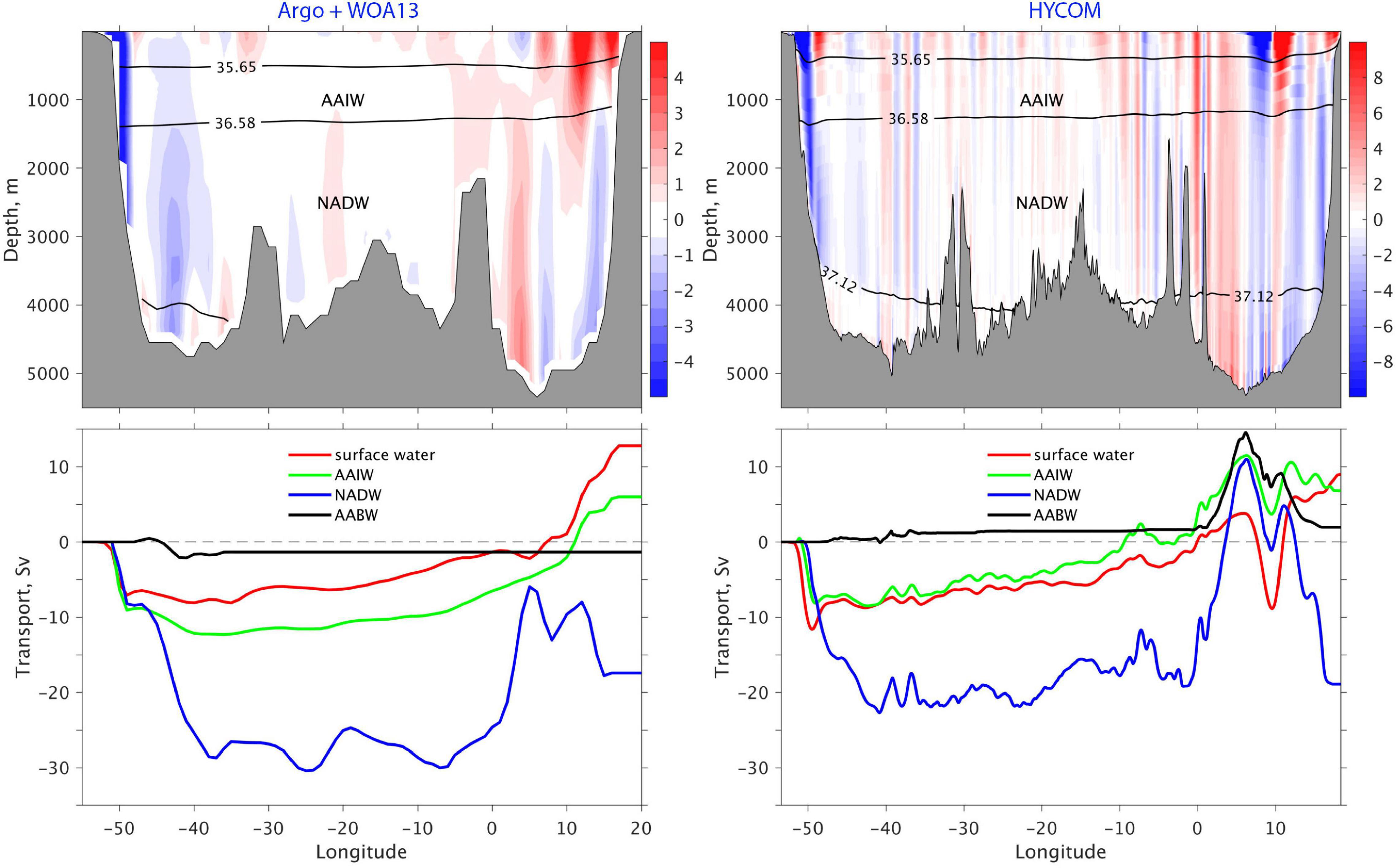
Figure 4. Observed and modeled time mean meridional velocity (color shading in cm/s) across 34°S and the corresponding volume transport for the four density layers: near surface water (σ₂< 35.65 kg m^–3), Antarctic Intermediate Water (AAIW, 35.65 < σ₂< 36.58), North Atlantic Deep Water (NADW, 36.58 < σ₂< 37.12), and Antarctic Bottom Water (AABW, σ₂> 37.12). Observations are based on a combination of Argo-WOA13 profiles; model results based on the global 1/12° HYCOM simulation.

The meridional flows across 34.5°S as shown in Figure 4 have a significant barotropic component, and the baroclinic nature of the AMOC, i.e., northward flows in the upper limb and southward flows in the lower limb, becomes apparent only when integrated across the basin (Figure 5). The zonally integrated mean transport streamfunction with respect to the depth z shows a maximum overturning depth near 1300 m in both observations and model results (Figure 5A). The modeled mean AMOC transport is 14.7 Sv. This value agrees with the SAMOC estimate based on six years of two moored observations at the western and eastern boundaries (14.7 Sv, Meinen et al., 2018), but is significantly lower than the estimates based on nine moorings across the 34.5°S (17.3 Sv, Kersalé et al., 2020), XBT transects (18 Sv, Dong et al., 2009; Garzoli et al., 2013) and Argo-WOA13 (20 Sv, Dong et al., 2014). With respect to density (Figure 5B), the northward AMOC limb is above the density surface (σ₂) 36.58 kg/m³ and the southward limb below. The modeled mean AMOC transport in density space is 15.8 Sv, compared to 18.7 Sv based on Argo-WOA13 observations. The modeled northward AMOC limb consists of 9.0 Sv warm surface water and 6.8 Sv AAIW, compared to 12.7 and 6.0 Sv, respectively, in the Argo-WOA13. This leads to a lower meridional heat transport (MHT) of 0.36 ± 0.23 PW in the model, compared to 0.68 ± 0.24 PW in the Argo-WOA13. The historical estimates of the MHT near this latitude are 0.22–0.62 PW (see Table 29.3 in Macdonald and Baringer, 2013).

FIGURE 5

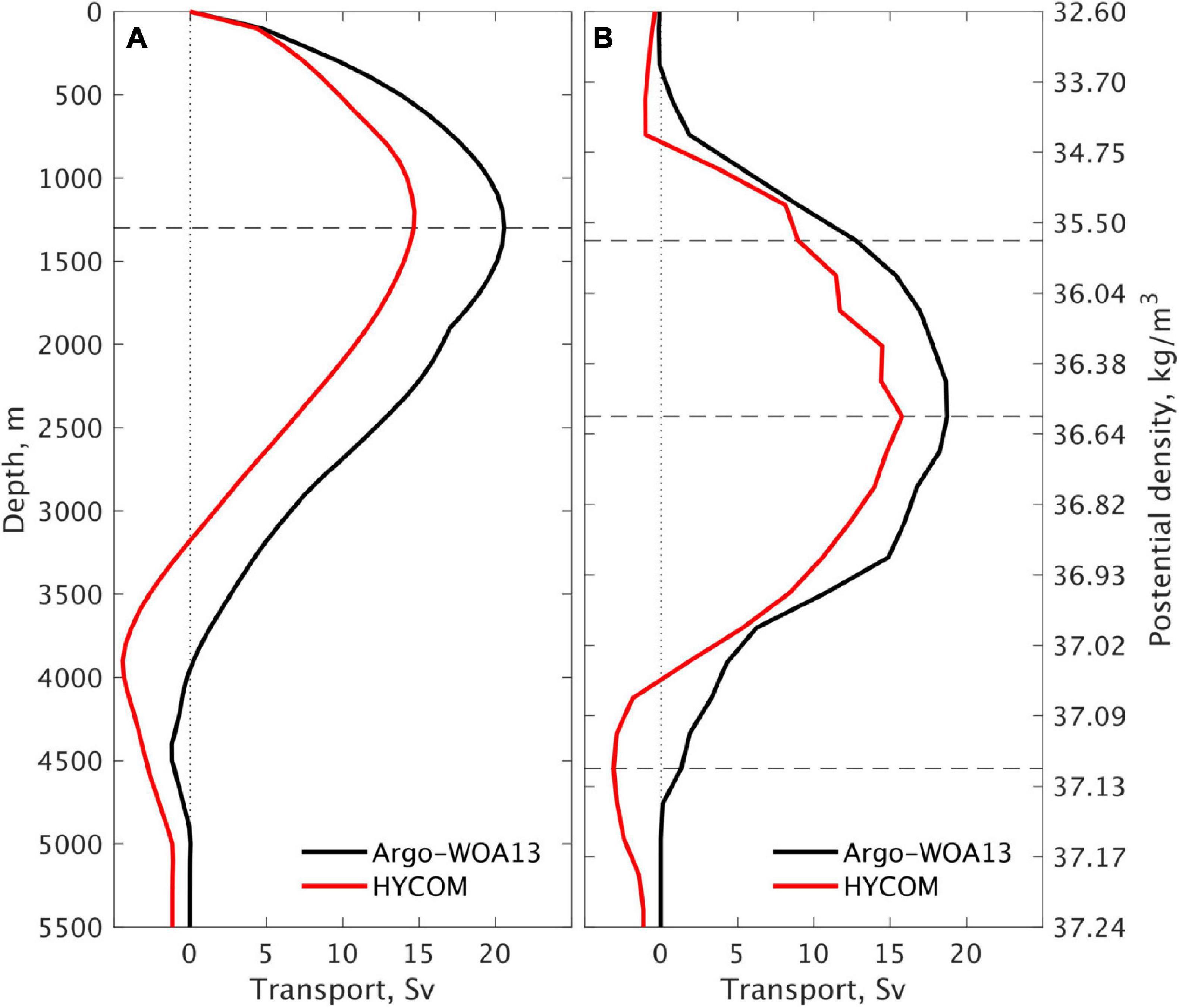
Figure 5. Long-term mean meridional overturning streamfunction (in Sv) at 34°S with respect to (A) depth and (B) potential density in σ₂. Observations based on monthly mean Argo-WOA13 profiles; model results based a global 1/12° HYCOM simulation (1979–2018).

At 34°S, the modeled AMOC transport variability is lower than observations on both interannual and seasonal timescales (Figure 6). On interannual timescale, the model AMOC transports have a standard deviation of 1.0 Sv in 2004–2014, compared to 1.9 Sv in Argo-WOA13 observations for the same period and 2.6 Sv in SAMOC results (Meinen et al., 2018) for a shorter, 6-year period (2009–2010 and 2013–2017). The time evolution of the modeled AMOC variability is similar to the Argo-WOA13 based observations in 2004–2012 but differ after 2012 (Figure 6A); note the Argo-WOA13 and SAMOC observations also differ in 2013–2014 when the two observations overlap. On seasonal timescale, the modeled AMOC transports have a standard deviation of 2.2 Sv, compared to 3.3 Sv in the Argo-WOA13 and 2.9 Sv in the SAMOC observations. Although the magnitude is lower, the phase of the modeled seasonal variability is consistent with the Argo-WOA13 and the SAMOC observations (Figure 6B).

FIGURE 6

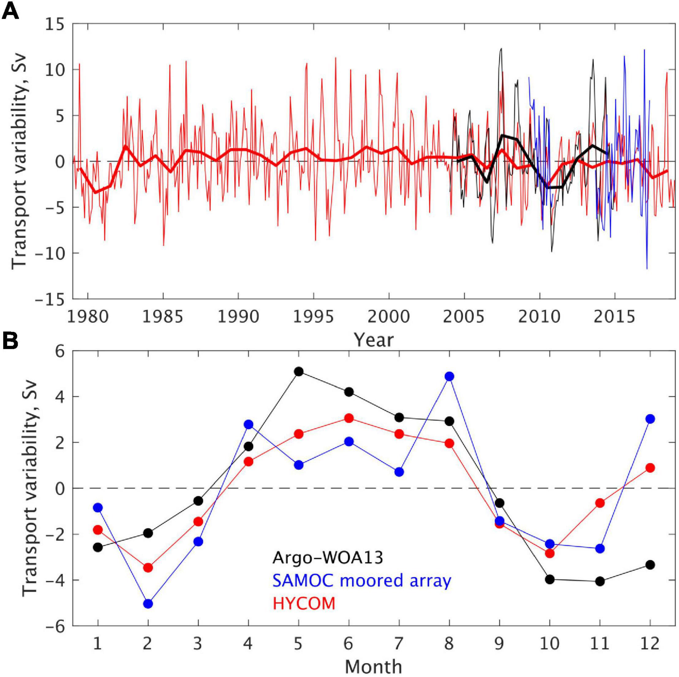
Figure 6. (A) Time series of the AMOC transport variability (in Sv) at 34°S based on Argo-WOA13 (black, Dong et al., 2014), SAMOC-mooring array (blue, Meinen et al., 2018), and global HYCOM (red). The thin and thick lines represent monthly means and 12-month moving averages, respectively. (B) AMOC transport variability at seasonal timescale, with each dot representing the multi-year average of the monthly AMOC transport.

Transport Through the Drake Passage at 65°W

The Drake Passage is an ACC chokepoint and the place where long-term sustained monitoring programs have been conducted; see Meredith et al. (2011) for a review of historical observations. The canonical full-depth volume transport is 133.8 ± 11.2 Sv, based on year-long current meter mooring and cruise data obtained during the International Southern Ocean Studies (ISOS, Whitworth, 1983; Whitworth and Peterson, 1985). However, based on a combination of moored current meter data from the DRAKE program (2006–2009) and satellite altimetry data (1992–2012), Koenig et al. (2014) estimated a higher full-depth transport of 141 ± 2.7 Sv. More recently, Chidichimo et al. (2014) and Donohue et al. (2016) estimated an even higher mean ACC transport of 173.3 Sv, based on the high-resolution moored bottom current and pressure measurements of the cDrake program (2007–2011).

The modeled mean ACC transport is 157.3 Sv, about the average of the estimates from DRAKE and cDrake programs. In a detailed analysis of the modeled ACC transport through the Drake passage, Xu et al. (2020) found that (a) the modeled ACC transport in the upper 1000 m of the Drake Passage is in excellent agreement with that of Firing et al. (2011) based on shipboard acoustic Doppler current profiler (SADCP) transects, and (b) the modeled exponentially decaying transport profile is consistent with the profile derived from the repeat hydrographic data from Cunningham et al. (2003) and Meredith et al. (2011). By further comparing the model results to the cDrake and DRAKE observations, Xu et al. (2020) concluded that the modeled 157.3 Sv was representative of the time-mean ACC transport through Drake Passage. The cDrake experiment overestimated the barotropic contribution in part because the array under-sampled the deep recirculation in the southern part of the Drake Passage, whereas the DRAKE experiment underestimated the transport because the surface geostrophic currents yielded a weaker near-surface transport than implied by the SADCP data.

The modeled mean zonal velocity through the Drake Passage at 65°W and the corresponding volume transports for the four density layers defined earlier (surface water, AAIW, NADW, AABW) are shown in Figure 7A. The ACC at this longitude exhibits four high velocity cores (indicated by arrows in Figure 7A), corresponding to the ACC southern boundary (SBby, south of 63°S), the southern ACC Front (SACCF, at 61–62°S), the Polar Front (PF, at 58–60°S), and the Sub-Antarctic Front (SAF, at 56–58°S). These modeled fronts are at similar locations as in Orsi et al. (1995) based on hydrographic surveys and in other studies based on SSH data (e.g., Sallée et al., 2008; Sokolov and Rintoul, 2009; Kim and Orsi, 2014).

FIGURE 7

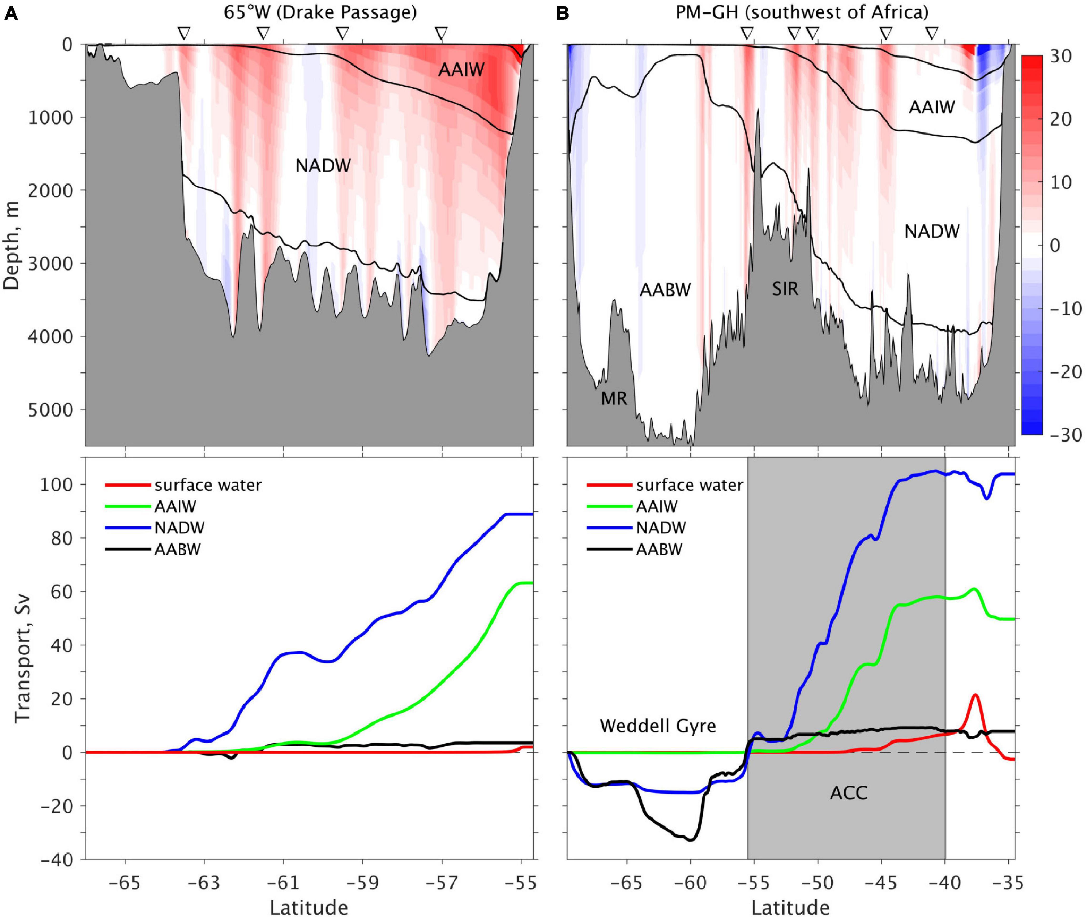
Figure 7. Modeled long-term mean zonal velocity and the corresponding four-layer volume transport in four density layers across (A) 65°W in the Drake Passage and (B) the Prime Meridian-Good Hope (PM-GH) transect southwest of Africa. The triangles denote the locations of Antarctic circumpolar current (ACC) fronts, from south to north, the Southern Boundary, South ACC Front, Polar Front, Subantarctic Front, and the subtropical front in panel (B). The shaded area in panel (B) between 40 and 55.5°S marks the ACC regime across the PM-GH transect. Transport is accumulative northward. The four layers are near surface water (σ₂ < 35.65 kg m^–3), Antarctic Intermediate Water (AAIW, 35.65 < σ₂ < 36.58), North Atlantic Deep Water (NADW, 36.58 < σ₂ < 37.12), and Antarctic Bottom Water (AABW, σ₂ > 37.12).

The modeled monthly mean and 12-month moving averaged ACC transports have a standard deviation of 5.2 Sv and 2.3 Sv, respectively (panel a in Supplementary Figure 2). These numbers are relatively small compared to the long-term mean value of 157.3 Sv. The seasonal variability of the ACC transports is also small (with a standard deviation of 1.5 Sv) and exhibits a biannual pattern (panel b in Supplementary Figure 2). These results agree with the observations in Koenig et al. (2016).

Transport Across the Prime Meridian-Good Hope Transect

The wide ocean gap between Antarctica and the southern tip of Africa makes it difficult to fully measure the transport and its spatial structure. Observations have been collected mostly along the Prime Meridian (e.g., Whitworth and Nowlin, 1987; Klatt et al., 2005) from Antarctica to approximately 50°S and the Good Hope line from 0°E, 50°S to the Cape of Good Hope, South Africa (e.g., Legeais et al., 2005; Gladyshev et al., 2008; Swart et al., 2008). We refer to the combination of these two sections as the Prime Meridian-Good Hope (PM-GH) transect (Figure 1). The modeled net transport through PM-GH (158.5 Sv) is essentially the same as the net transport through the Drake Passage because of mass conservation, except for an additional 1.2 Sv from the Pacific-to-Atlantic Bering Strait throughflow.

The modeled circulation along the PM-GH section (Figure 7B) can be divided into three regimes:

i) Weddell gyre south of 55.5°S. There are two eastward and two westward jets that form the Weddell gyre. The two westward jets are found along the Antarctic Slope and the Maud Rise (MR) near 64°S, whereas the two eastward jets are found near 58–59°S and along the southern boundary (SBdy) of the ACC at 55.5°S right south of the Southwest Indian Ridge (SIR). This modeled jet pattern is consistent with the observations of Klatt et al. (2005, their Figures 4, 5). The time mean transport of the modeled Weddell gyre is 48.2 Sv, compared to 56 ± 8 Sv estimated in Klatt et al. (2005).

ii) ACC from 55.5 to 40°S. The modeled ACC exhibits high-velocity cores associated with the SACCF (52°S), PF (50.4°S and 48°S), SAF (44.6°S), and the subtropical front (STF, 42°S) respectively. These front positions are close to the observations based on repeat CTD/XBT transects in this region (Swart et al., 2008, their Table 3). Note that the PF at this location is split into two fronts, with the elevated eastward velocity between 47 and 49°S corresponding to its northern expression (Gladyshev et al., 2008; Swart et al., 2008). The modeled STF is much weaker than any of the other ACC fronts as in the observations. The modeled mean ACC transport across the PM-GH transect, defined as the transport from 55.5 to 40°S including the STF as in Orsi et al. (1995), is 175 Sv, compared to 147-162 Sv estimated from CTD transects (Whitworth and Nowlin, 1987; Legeais et al., 2005; Gladyshev et al., 2008). The modeled baroclinic transport is 101.2 Sv above 2500 m, compared to 84.7–97.5 Sv derived from repeated hydrographic surveys and in combination with satellite altimetry data (Legeais et al., 2005; Swart et al., 2008).

iii) Agulhas retroflection and leakage north of 40°S. The model results show a pair of eastward and westward flows associated with the Agulhas retroflection and Agulhas Current. Slightly upstream at 28°E, the modeled full-depth Agulhas Current transport is 86.2 Sv, which is close to the observational estimate of 84 Sv in Beal et al. (2015). The “net” transports north of 40°S is 9.3 and 7.9 Sv westward for the surface water and AAIW, respectively. Thus, the Agulhas leakage in model provides slightly more transport than the 15.8 Sv in upper AMOC at 34°S.

The modeled transport across the full PM-GH transect decreases with depth and is eastward above 4000 m (blue line in Figure 8A). There is a weak westward flow below 4000 m. When compared to the vertical structure of the transport in the Drake Passage (green line in Figure 8A), the eastward transport through PM-GH transect is weaker in the 0–1000 m range and stronger in the 1000–4000 m range. This is due, in a large part, to the contributions to the northward-flowing upper limb and from the southward-flowing lower limb of the AMOC (red line in Figure 8A).

FIGURE 8

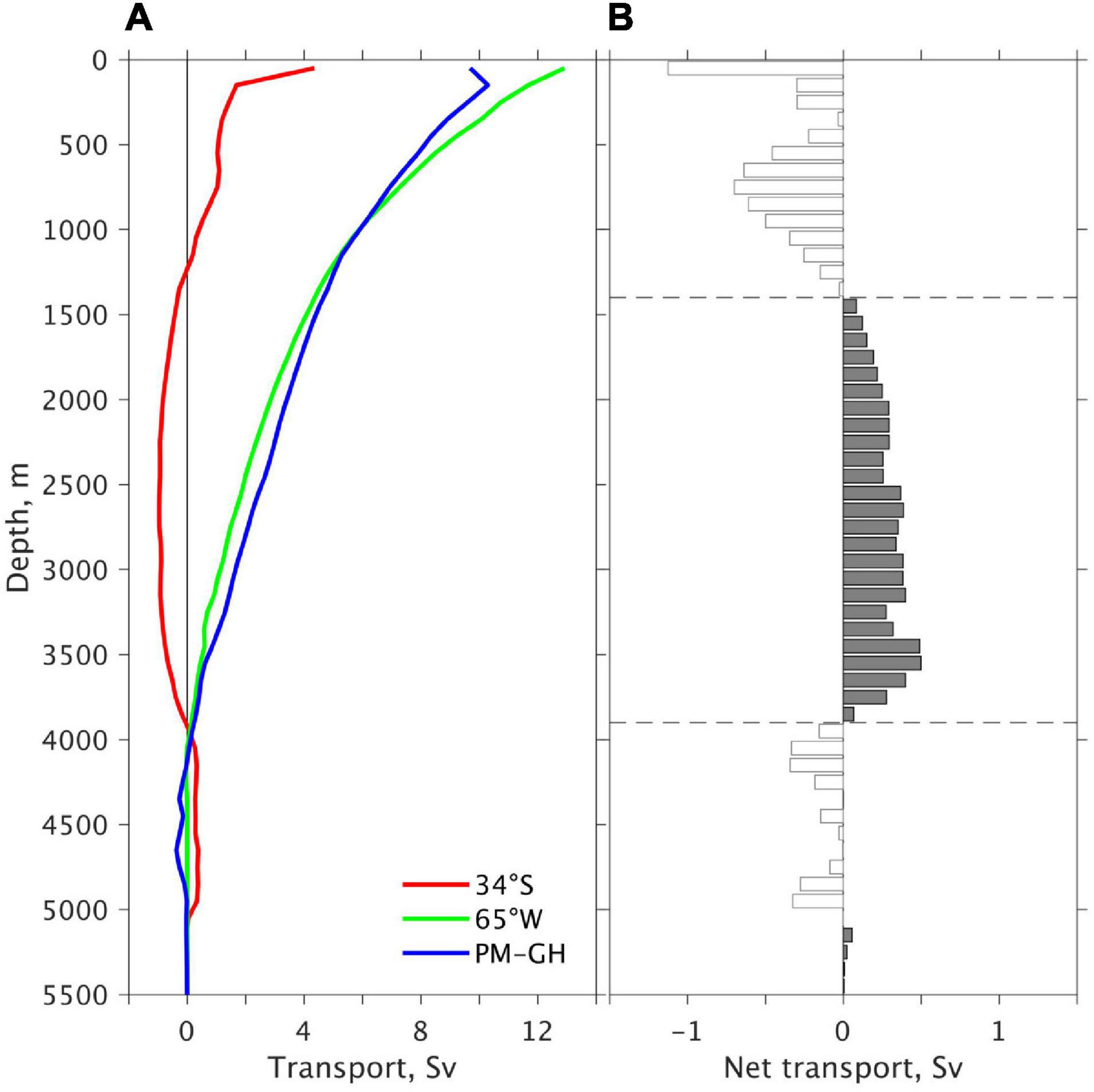
Figure 8. (A) Modeled mean horizontal transports (Sv per 100 m) in the vertical across the 34°S, the 65°W, and the PM-GH transects; (B) The net transports into the region enclosed by the three transects, with positive (negative) values indicating net transport into (out of) the region.

The modeled net transports into and out of the region bounded by the 34°S, Drake Passage, and PM-GH sections (see Figure 1) are shown in Figure 8B. There is a net outflow above 1400 m and below 3900 m and a net inflow between these two depths. The result implies a maximum upwelling transport of 5.6 Sv across 1400 m, consistent with the picture put forward by Schmitz (1995) and Talley (2013) that the Southern Ocean is a key upwelling region for NADW. The net transport in Figure 8B also implies a downward transport of 1.7 Sv across 3900 m, representing AABW formation in the model within the region bounded by the 34°S, Drake Passage, and PM-GH sections.

Circulation Pathways in the South Atlantic Ocean

In the previous section, we showed that the model is able to represent the basic circulation features of the South Atlantic and the Southern Ocean, and that the modeled volume transports are consistent with observations. In this section, we use the model results to address the questions raised in the introduction on the relative importance of the warm versus cold source water in the upper limb and the detailed circulation pathways of the lower limb of the AMOC.

Upper Limb (Surface Water and Antarctic Intermediate Water)

The upper (northward) limb of the AMOC consists of two density layers: the surface water (σ₂ < 35.65) and the AAIW (35.65 < σ₂< 36.58 kg m^–3). The modeled 40-year (1979–2018) mean horizontal circulation for these two layers is displayed in Figures 9, 10, respectively. For the surface water (Figure 9), the AMOC component flows directly northwestward from the Indian Ocean via the Agulhas Leakage into the South Atlantic (red streamlines); the subtropical gyre of the South Atlantic (orange lines) flows counter-clockwise and separates the northward-flowing AMOC component and the eastward-flowing ACC. There is almost no surface water in the ACC coming from the Pacific Ocean (pink lines) and it does not contribute directly to the AMOC.

FIGURE 9

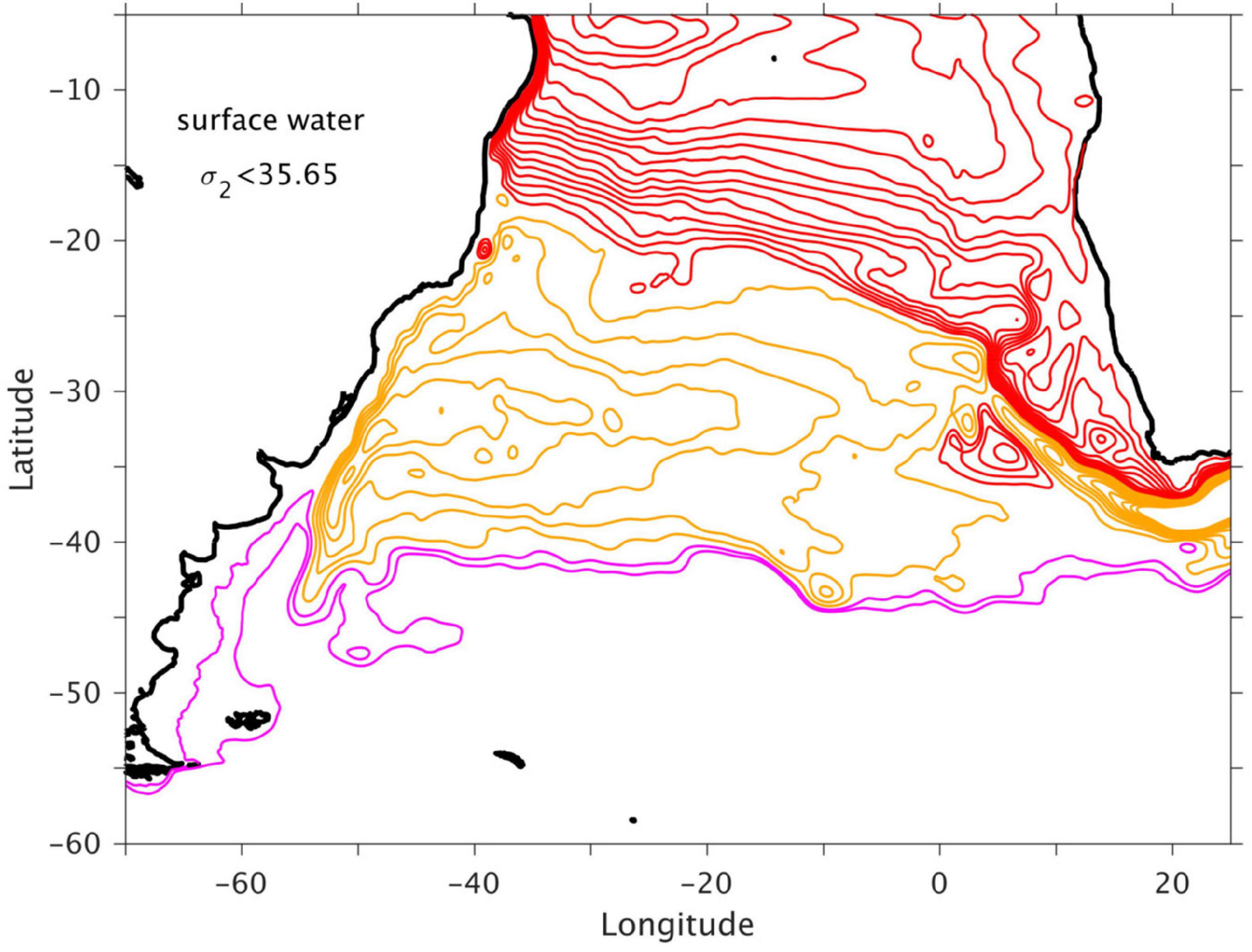
Figure 9. Modeled long-term mean horizontal transport streamfunction (in Sv) for the layer of near surface water (σ₂ < 35.65 kg m^–3). Red and pink streamlines (increment of 1 Sv) denote AMOC contribution and ACC flow; orange streamlines (increment of 2 Sv) denote the subtropical gyre of the South Atlantic.

FIGURE 10

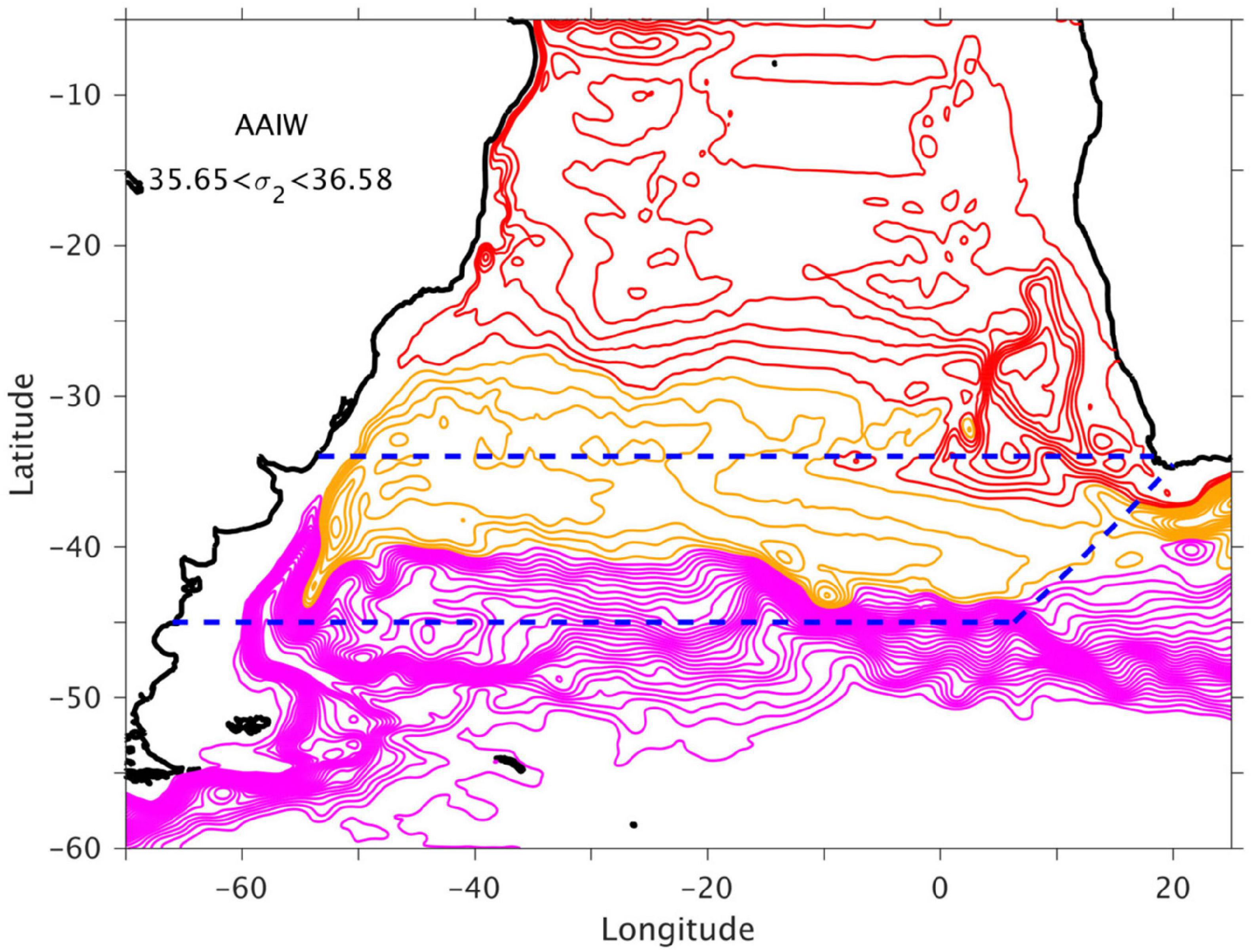
Figure 10. Modeled long-term mean horizontal transport streamfunction (Sv) for the layer of AAIW (35.65 < σ₂ < 36.58 kg m^–3). Pink streamlines (increment of 4 Sv) is the ACC; red and orange streamlines denote AMOC contribution and the subtropical gyre of the South Atlantic (similar to Figure 15). The dashed blue lines denote 34°S, 45°S, and the GoodHope sections, across which the water properties of the northward and northwestward transports are examined in Figure 14.

FIGURE 11

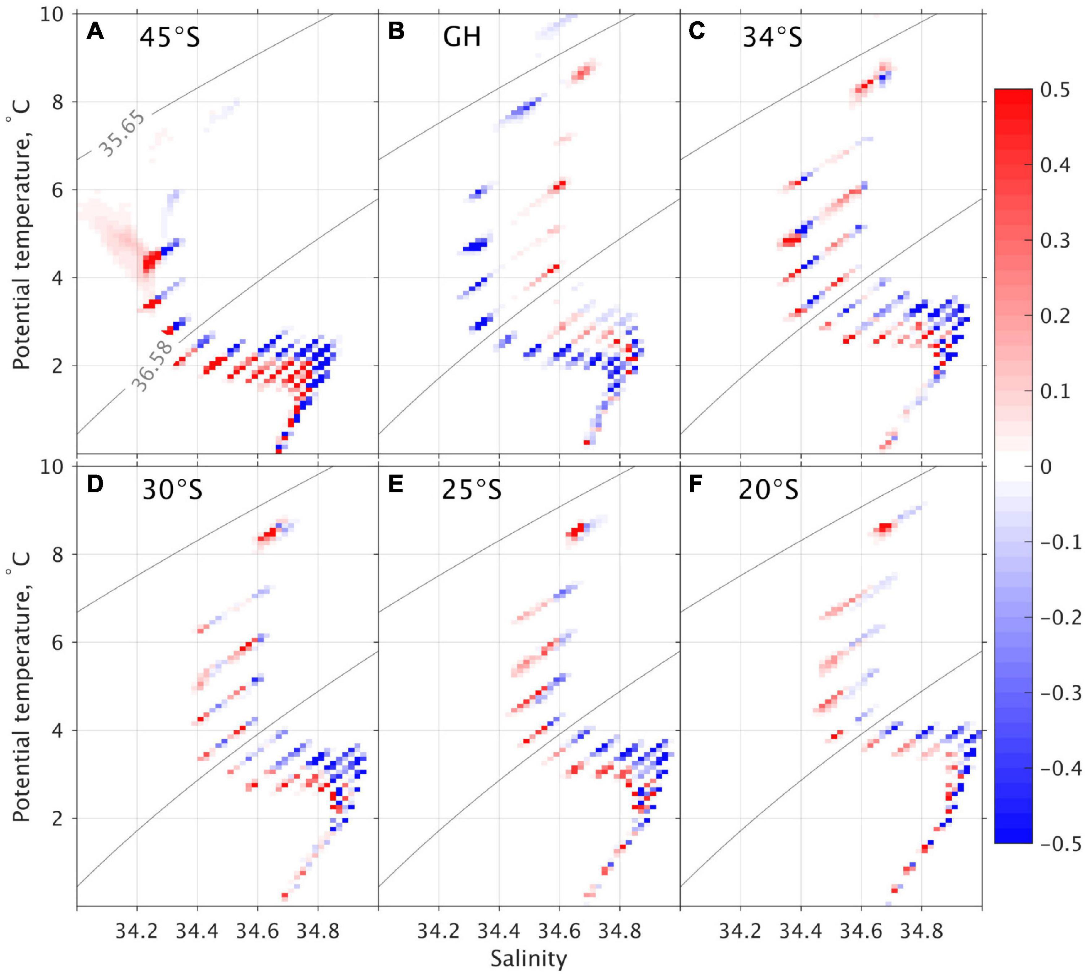
Figure 11. Modeled meridional transports projected on potential temperature-salinity (θ -S) plane across 6 sections (A–F: 45°S, GH section, 34°S, 30°S, 25°S, and 20°S, respectively), presented in Sv over an area of (0.2°C × 0.04) in θ -S space. The red and blue colors represent north and south transports into and out of the South Atlantic. The isopycnal (σ₂) surfaces of 35.65 and 36.58 kg m^–3 denote the upper and lower AAIW interfaces.

To further study the contribution of Pacific versus Indian AAIW not represented in the time-mean circulation, we released numerical particles into the model AAIW density layers in the North Brazil Current (NBC) along 6°S and tracked their trajectories backward using the modeled daily velocity fields and the Lagrangian Ocean analysis toolbox OceanParcels (Delandmeter and van Sebille, 2019). At this latitude, the NBC is a boundary current that can be well-defined from coast to 33°W and the modeled NBC transport (27.7 Sv) compares well to the observed value (26.5 Sv in Schott et al., 2005). The particles were released in the northward-flowing NBC along 6°S every month in 2017–2018 and were back-tracked for 30 years. Similar to Blanke et al. (1999) and Rühs et al. (2019), the number of particles released at each grid point on the section is proportional to the model transport at that location. Each particle is tacked with a small partial volume transport (∼0.01 Sv) such that the cumulative volume transport of all the particles reflects the instantaneous total AAIW transport through the NBC each time they are released. A total of 34,016 particles were released and the majority (23,683 or ∼70%) of these particles remains in the South Atlantic, mostly north of 30°S, after 30 years of integration. Out of the 10,333 particles that “exit” the South Atlantic, 3,166 (∼30%) were found to flow through the Drake Passage box first, i.e., the cold route, and 7,167 (∼70%) through the Agulhas Leakage, i.e., the warm route. Figures 12A,B display the probability that one particle went through a given location in the South Atlantic from the cold and warm routes to reach the NBC at 6°S during the 30-year integration. The high probability area of cold-route particles (in Figure 12A) between 30 and 40°S resembles the shape of time-mean streamline of the subtropical gyre (orange contours in Figure 10). It indicates that, through transient eddies, particles from the ACC enter the subtropical gyre near the Malvinas confluence zone and exit the subtropical gyre into the AMOC near 30°S, 30°W. The high probability area of the warm-route particles (Figure 12B) follows the translation pathway of Agulhas Rings: northwestward through the Cape Basin, then zonally across the South Atlantic near 25–30°S, before turning northward into the western boundary current that feeds into the NBC. This pathway is in general agreement with the time mean AAIW streamlines that contribute to the AMOC in Figure 10 (red contours). Figures 12C,D displays the time scales taken by the particles from the Drake Passage and the Agulhas Leakage to reach the NBC along 6°S. The most common time for a particle to reach 6°S is about 18 and 12 years, respectively, from the Drake Passage and the Agulhas Leakage (both routes exhibit a wide range of time scales).

FIGURE 12

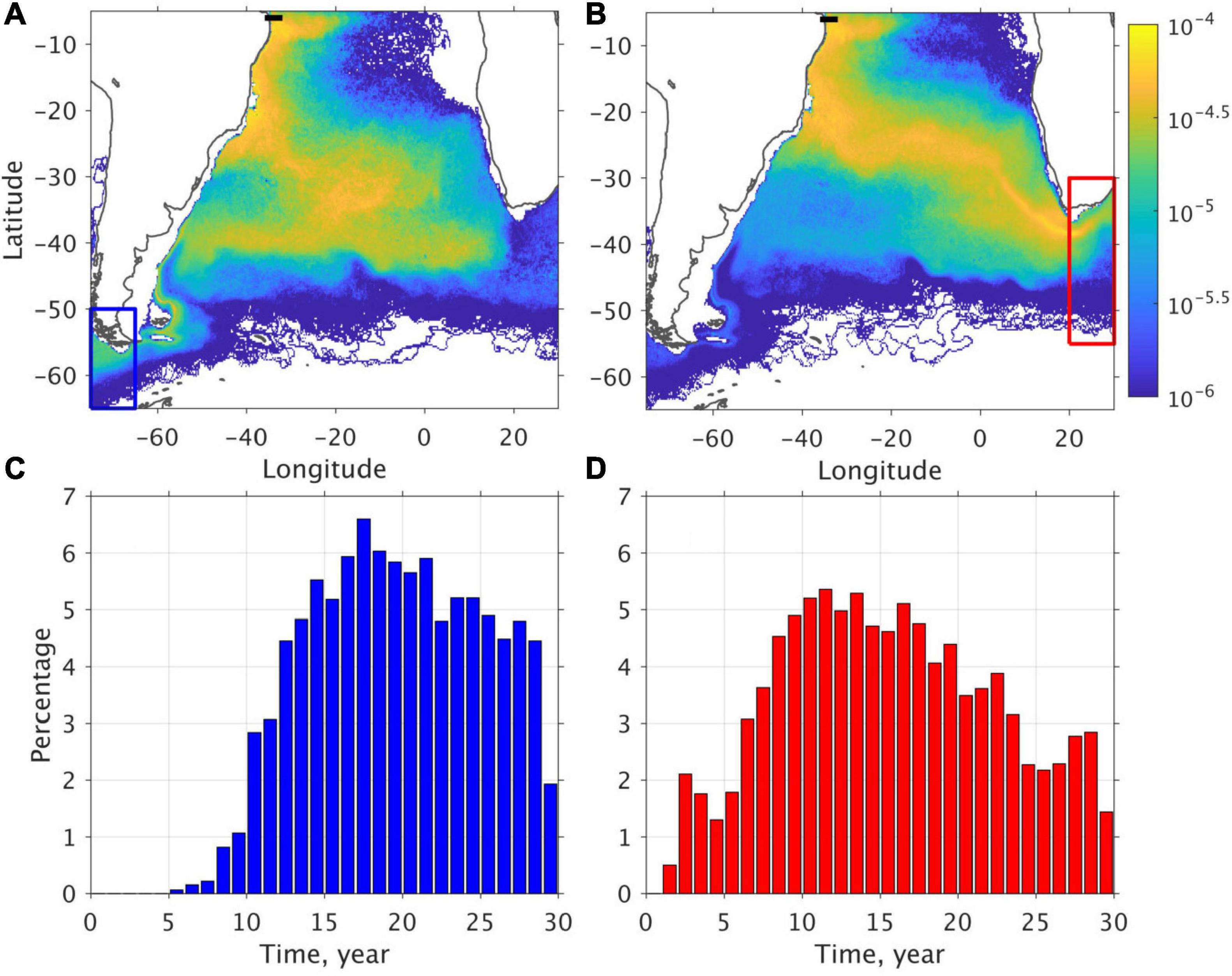
Figure 12. (A,B) Probability map of the trajectory occurrence in the South Atlantic (1/4° × 1/4° grid) for the AAIW particles that were released along 6°S in the North Brazil Current (thick black line) and back-tracked for 30 year to reach (A) blue box in the Drake Passage (3,166 particles) and (B) red box in the Agulhas Leakage (7,167 particles); (C,D) the percentage of the particles that were back-tracked to reach (C) the Drake Passage and (D) the Agulhas Leakage as a function of time. The probabilities are computed as the number of particles landing in 1/4°x1/4° box normalized by total number of particles over time.

FIGURE 13

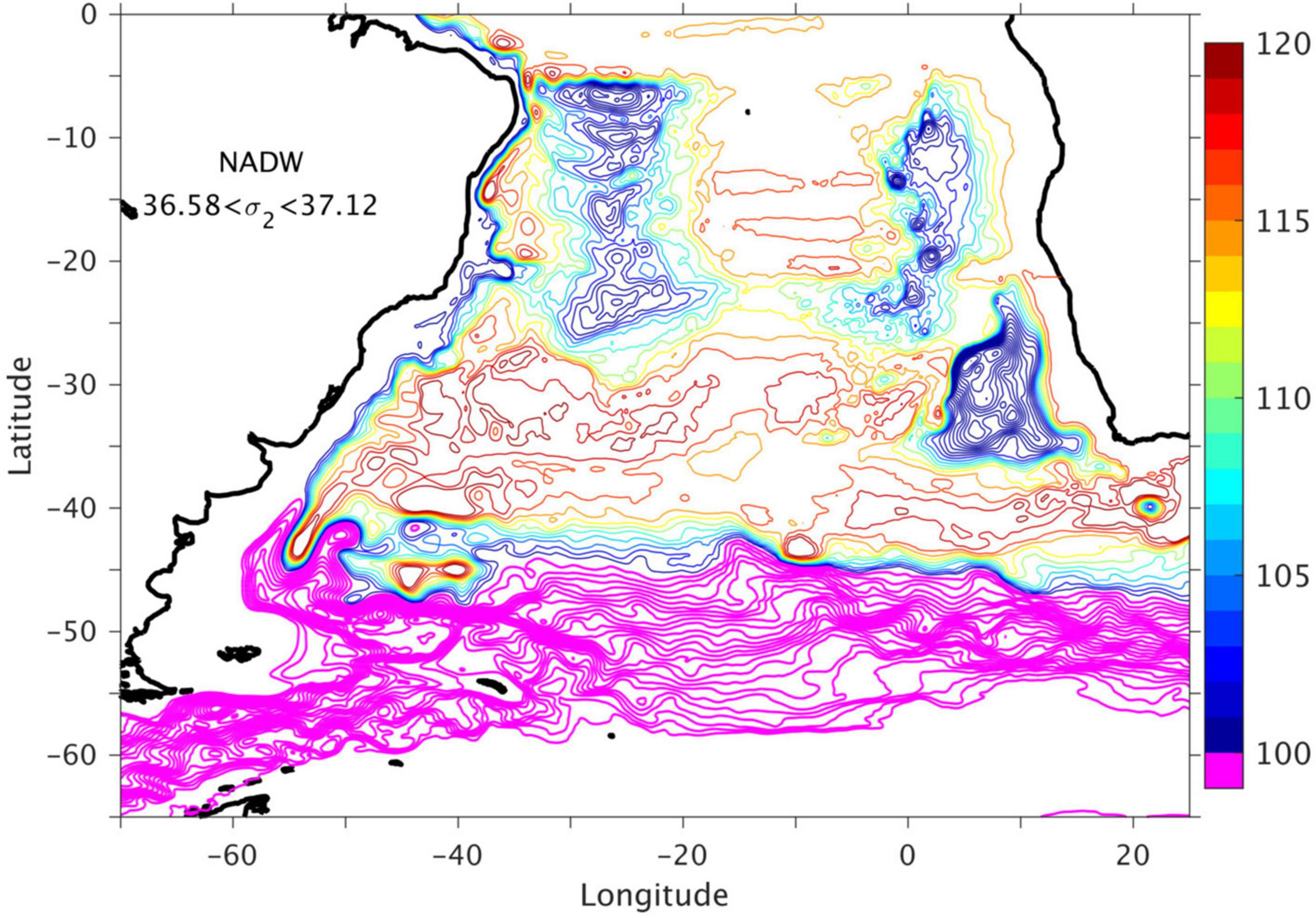
Figure 13. Modeled long-term mean horizontal transport streamfunction for the layer of NADW (36.58 < σ₂ < 37.12 kg m^–3). Pink streamlines (4 Sv increment) indicate the eastward transport of the ACC, blue to yellow streamlines (2 Sv increment) represent the southward spreading of the NADW from north.

FIGURE 14

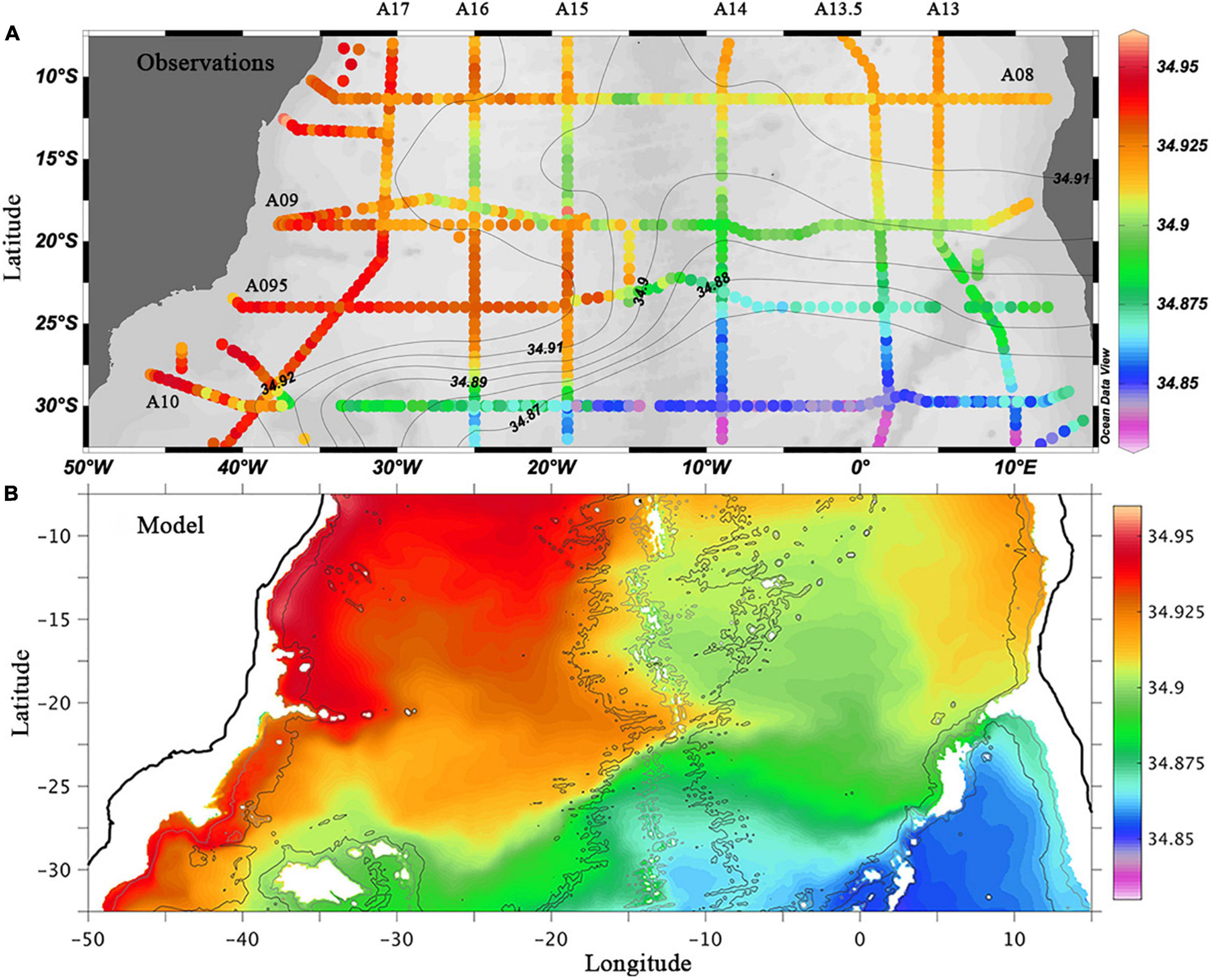
Figure 14. Observed and modeled salinity distribution at 2500m in the South Atlantic. Observations are based on CTD data from GoShip program http://www.go-ship.org. Detailed vertical sections can be seen in the WOCE Atlas (Koltermann et al., 2011). The results show an eastward extension of high salinity (NADW signature) between 20 and 25°S west of the mid-Atlantic Ridge (MAR), and significantly lower salinity east of MAR.

FIGURE 15

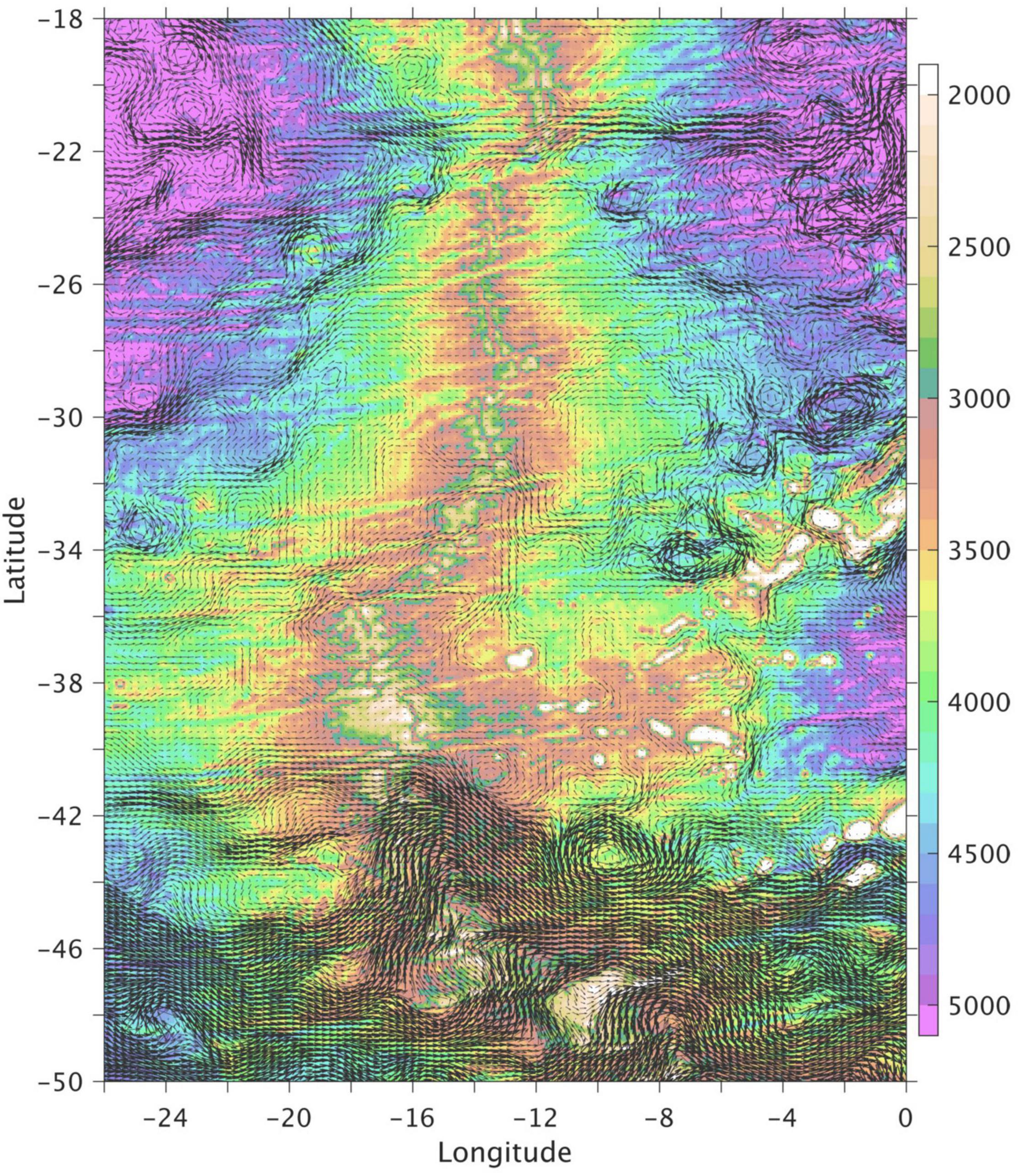
Figure 15. Zoomed view of the modeled mean circulation for the density layer of NADW (36.58 < σ₂ < 37.12 kg m^–3) across the Mid-Atlantic Ridge in the South Atlantic Ocean.

The modeled circulation pattern of the AAIW (Figure 10) is similar to the surface water (Figure 9), but it shows a meridionally more confined subtropical gyre (orange lines) and a larger contribution to the ACC from the Pacific Ocean (pink lines). There is an indication of a “supergyre” connecting the subtropical gyres of the South Atlantic and Indian Oceans, which would further prevent a direct contribution of water mass from the ACC into the upper limb of the AMOC. The patterns of modeled mean circulation in Figures 9, 10 are similar to the schematic of Stramma and England (1999, their Figures 3, 4), except for the recirculation in the Cape Basin which is a consequence of the unrealistic pathways of the modeled Agulhas eddies (see Figure 2 and Supplementary Figure 1 as well as discussion in subsection “Surface circulation pattern”).

The model time-mean circulation in Figure 10 suggests that the Pacific AAIW does not directly contribute to the upper limb of the AMOC. But this does not necessarily imply that there is no contribution by the time-varying part of the circulation, e.g., eddies and meanders. To quantify the combined contribution of the mean flow and eddies by the various water mass sources, we examine the water properties of the northward flow in the South Atlantic, by projecting the meridional transports (in Sv) on potential temperature-salinity (θ-S) plane and comparing their properties with the water masses from the Pacific and the Indian Oceans (Figure 11). The Pacific AAIW that flows northward across 45°S is much fresher than the Indian AAIW that flows westward across the GH section (Figures 11A,B). The AAIW that flows northward across 34°S and 30°S is a combination of these two sources (Figures 11C,D): At 34°S, 7.8 Sv of AAIW is fresher than 34.46 (Pacific) and 9.6 Sv is saltier than 34.46 (Indian). At 30°S, the Pacific contribution (S < 34.46) decreased to 3.6 Sv whereas the Indian contribution stayed approximately constant at 9.0 Sv. Further north at 25°S and 20°S (Figures 11E,F), the Pacific origin cannot be identified in the θ -S diagram, suggesting that the main contribution of the Pacific AAIW in the South Atlantic is to the subtropical gyre, not to the AMOC. However, the northward-flowing AAIW at 20–25°S is fresher than that at GH (the transport-weighted AAIW salinity is 34.56 at 20–25°S versus 34.60 at GH). This implies that mixing between the Indian and Pacific AAIWs takes place in the South Atlantic. In addition to this (isopycnic) mixing between the two different AAIW sources, there is also (diapycnal) mixing/water mass transformation between the AAIW and the near surface water that occurs in the South Atlantic. Supplementary Figure 3 displays the spatial distribution of the mean AMOC transport and the AAIW and near surface water contributions. The results show that about 1.8 Sv of AAIW is transformed into near surface water between 25 and 5°S with a small decrease in overall AMOC transport of ∼1 Sv between 34 and 5°S.

The volume transport carried by all the particles divided by the number of releases provides an annual mean “Lagrangian” AAIW transport for each route: 1.3 Sv for the cold route (30%) and 3.0 Sv for the warm route (70%). The sum of these two transports (4.3 Sv) is slightly lower than the “Eulerian” 5 Sv mean transport of AAIW across 6°S (Supplementary Figure 3). The most useful result out of the Lagrangian experiment is not the absolute transport of each route, but the ratio between the two, since many of the particles have not yet left the South Atlantic at the end of the 30-year integration and a steady state has not been reached. If one assumes that the 5.0 Sv AAIW that flows across 6°S has the warm-to-cold contribution ratio (30% to 70%) as indicated by the Lagrangian particles, then the cold and warm-route AAIW contributions are about 1.5 Sv and 3.5 Sv, respectively. Finally, only about ∼2 Sv of the Drake Passage transport is in the surface water density range (Figure 7A), hence the surface water contribution from Drake Passage (to the AMOC) is likely negligible. Therefore, our cold-route contribution is in the order of 1.5 Sv. This is about 1/3 of the 4.7 Sv as estimated by Rühs et al. (2019) using a nested high-resolution ocean simulation. It is, however, higher than the recent estimate of 0.4 Sv by Rousselet et al. (2020) that is derived using the ECCOv4 (Estimating the Circulation and Climate of the Ocean). Note we have only considered direct contributions in this study. Some Pacific water could flow into Indian Ocean first and mix with the Indian waters before contributing to AMOC through the Agulhas Leakage (Speich et al., 2001, 2007), those would be considered as warm-route contribution.

Lower Limb (North Atlantic Deep Water)

Figure 13 shows the modeled mean circulation for the NADW layer (36.58 < σ₂< 37.12). The modeled NADW flows southward as a DWBC along the continental slope of the Brazil and Argentine Basins, all the way to about 40°S where it encounters the northward-flowing deep Falkland Current. The NADW continues to flow southward (now offshore of the deep Falkland Current) to about 45°S where it meanders and flows eastward south of the Zapiola Drift. This modeled NADW pathway is similar to the one described in the schematic of Stramma and England (1999, their Figure 5) and is consistent with pathways derived from salinity, oxygen, and other tracers such as CFC (e.g., Koltermann et al., 2011; Garzoli et al., 2015). It is also similar to the typical NADW pathway reconstructed from Lagrangian trajectories in Rousselet et al. (2021) using reanalysis results. There is a strong counterclockwise flow around the Zapiola Drift (Figure 13) with a transport of approximately 25 Sv. The Zapiola anticyclone extends from surface all the way to the bottom, and the modeled time mean full water column transport is about 55 Sv, which is consistent with 50 Sv estimated in Saraceno et al. (2009) using the mean dynamic topography (MDT) data. The transport is highly variable, however, with a standard deviation value of 33 and 18 Sv for the monthly and annual means, respectively. Given the high variability (on intraseaonal and interannual scales), it is not surprising that significantly higher transports have been estimated, e.g., 80 Sv by Saunders and King (1995) from CTD/ADCP data and 124 Sv by Colin de Verdière and Ollitrault (2016) from Argo float data.

In addition to the DWBC, the modeled NADW layer streamfunction (Figure 13) suggests complex recirculation patterns in the Brazil Basin, the Angola Basin, and the Cape Basin, contrast with the smooth streamfunction pattern derived from Lagrangian studies using coarse resolution model and reanalysis (Speich et al., 2007; Rousselet et al., 2021). Hogg and Owens (1999) documented the NADW recirculation in the Brazil Basin using sub-surface float data. Their results show strong zonal flows in the interior, especially near 5–10°S and around the Vitoria-Trindade Seamount Chain near 20–25°S. These zonal flows carry NADW from the DWBC toward the interior and lead to high salinity all the way to the MAR in both the observations (WOCE lines A09 and A095) and the model (Figure 14). The modeled recirculation within the Cape Basin as discussed in Section “Water mass and transport across 34^°S” is consistent with the observations. There is no direct observation on the Angola Basin deep circulation, but the modeled clockwise recirculation is consistent with the inverse calculation by Hogg and Thurnherr (2005) and the water property distribution.

The model exhibits a zonal flow of about 2 Sv across the MAR near 22°S (Figures 13, 15), which agrees with the 2–5 Sv estimated from observations by Warren and Speer (1991), Speer et al. (1995), Hogg and Thurnherr (2005), and Garzoli et al. (2015). East of the MAR, the modeled NADW flow turns northward and circulates around the Angola Basin as in the schematic proposed by Hogg and Thurnherr (2005). Arhan et al. (2003), however, proposed a much higher transport (10.7 Sv) of NADW that flows eastward across the southern Angola Basin and southeastward into the Cape Basin. Both the observed and modeled salinity distributions at 2500 m (Figure 14) show that between 20 and 25°S, there is a large salinity difference between the east and west of the MAR (A15 and A14 WOCE lines, respectively). This does not support Arhan et al. (2003)’s depiction of a high-salinity NADW transport across the MAR all the way to the eastern boundary. In a numerical study performed with the JAMSTEC OFES (OGCM for the Earth Simulator) model, van Sebille et al. (2012) did find a continuous NADW flow east of the MAR, but this leads to a continuous high salinity tongue (not shown) that extends eastward across the entire Angola Basin and southeastward into the Cape Basin, a result that is not supported by the observations.

Figure 15 also shows that in NADW density range there are weak westward currents across the MAR south of 22°S which lead to a lower salinity (modeled and observed) in the west basin near 30°S (along A10) when compared to 20–25°S (A09 and A095). Overall, there is no net transport of NADW across the MAR between 20 and 40°S, thus most of the eastward NADW transport occurs near 42°S where it joins the ACC water of the same density range (36.58 < σ₂< 37.12). The NADW/ACC streamlines turn northward when approaching the MAR and southward after crossing the MAR. This meridional shift can be explained by the conservation of potential vorticity, f/h, i.e., a decrease in thickness h when approaching the MAR leads to a northward shift to reduce the planetary rotation f so that f/h is constant and vice versa. Because the MAR is slanted in a northwest-to-southeast direction in this area, the northward and southward shifts at different latitude/longitude led to a contraction of the streamlines near 10°W, which can be clearly seen in the SSH for both model and observations (Figure 2).

Summary and Discussion

Through the South Atlantic Ocean, the AMOC is connected to the Indian/Pacific Oceans and is entangled into the global overturning circulation system. This important region is also particularly complex, featuring strong boundary currents (jets) and high eddy variability in both the western and eastern boundaries as well as in the Atlantic sector of the Southern Ocean. Observations of the full-depth circulation structure are focused on limited places, thus the three-dimensional circulation structure in the South Atlantic and the large-scale pattern of the AMOC variability are not well-determined. In this study, we used numerical results from a long-term 1/12° global simulation, along with observations, to address the questions on the mean circulation pattern that cannot be addressed using only observations. The model results are shown to represent well the transports and the vertical structure of the key circulation patterns in this region, especially, the AMOC across 34°S in the South Atlantic, the ACC at 65°W in the Drake Passage, as well as the zonal flows along the PM-GH transect in the open ocean southwest of Africa. The key results, derived from Lagrangian and Eulerian analyses, are:

1) The Pacific AAIW plays a significant role in setting the temperature and salinity properties of the water in the subtropical South Atlantic, but the upper limb of the AMOC is found to primarily originate from the warm Indian water through the Agulhas leakage (9.8 Sv surface water + 3.5 Sv AAIW) and only a relatively small contribution of 1.5 Sv colder, fresher AAIW originates from the Pacific Ocean through the Drake Passage.

2) In the lower limb of the AMOC, the NADW flows southward in the DWBC along the continental slope and in complex recirculation in the Brazil Basin, especially around the Vitória-Trindade Seamount Chain near 20°S. The recirculation carries the NADW and its high-salinity signature into the offshore interior. A weak zonal flow of NADW of ∼2 Sv is found to cross the MAR near 22°S. Different from the schematic of Arhan et al. (2003) based on inverse model and the previous numerical results of van Sebille et al. (2012), however, this modeled NADW does not continue to flow eastward across the Angola Basin and southeastward into the Cape Basin. Instead, it turns northward and circulates around the Angola Basin like the schematic proposed by Hogg and Thurnherr (2005). This NADW circulation pattern is consistent with the water property distribution, i.e., in both observations and model, the salinity east of MAR is significantly lower than that to the west. Virtually all of the NADW from the north flows in the DWBC all the way to 40–45°S before turning eastward to flow across the MAR near 42°S, 10°W. This crossing has a surface signature of concentrated SSH contours and is visible in satellite observations.

Although the modeled transport and vertical structure of the South Atlantic presented in this study are largely consistent with the observations, there is room for improvement. In particular, the modeled Agulhas Rings dissipate too slow and follow a regular pathway. This leads to a high EKE tongue that extends much farther to the northwest and impacts the regional circulation pattern in the eastern South Atlantic. Several remedies have been put forward to improve the realism of the circulation in the Agulhas region, namely (i) using finer horizontal resolution along with a better representation of the bathymetry features like the Agulhas Bank/Plateau as well as the continental slope and seamounts (Speich et al., 2006); (ii) using a higher order advection scheme which would lead to more irregularity in Agulhas eddy size and pathway (Backeberg et al., 2009), or (iii) including the ocean current feedback in the wind stress calculation (Renault et al., 2017; Chassignet et al., 2020). While it is indeed more physical to take into account the vertical shear between atmospheric winds and ocean currents when computing the wind stress, it does lead to an eddy damping effect that can reduce the kinetic energy by as much as 30% and a serious underestimation of EKE elsewhere in the domain (Chassignet et al., 2020). There is therefore a trade-off between a better representation of one current system (the Agulhas) and more realistic energetic and/or variability throughout the globe. A future comparison study is merited to evaluate the extent to which an improved Agulhas eddy presentation could impact the transport structure in the South Atlantic Ocean, through the interaction between the Agulhas eddies and the subtropical gyre and the exchange/mixing between warm and cold water along the eddy pathways.

Data Availability Statement

The altimeter products used here were produced by Ssalto/Duacs and distributed by AVISO, with support from CNES (http://www.aviso.altimetry.fr/duacs); the gridded T/S fields from the Argo float measurements are available at http://www.argo.ucsd.edu; the World Ocean Atlas 2013 is available at http://www.nodc.noaa.gov/OC5/woa13; the original global model outputs are stored in the ERDC archive server and the model results presented in this study are available in HYCOM server (https://data.hycom.org/pub/xbxu/GLBb0.08/SATLx). Further inquiries can be directed to the corresponding author.

Author Contributions

XX configured and performed the global simulation and analysis of the model results. EC coordinated the model configuration and analysis. SD and MB provided the observations and contributed on model-data comparison discussions. All authors participated in the interpretation of the results and in the writing of the manuscript.

Funding

This work was supported by the NOAA Climate Program Office MAPP Program (Award NA15OAR4310088), the NOAA Climate Variability and Predictability Program (Award GC16-210), and the Office of Naval Research (Grant N00014-19-1-2674). The numerical simulations were performed on supercomputers at the Engineer Research and Development Center (ERDC), Vicksburg, Mississippi, using computer time provided by the U.S. DoD High Performance Computing Modernization Program.

Conflict of Interest

The authors declare that the research was conducted in the absence of any commercial or financial relationships that could be construed as a potential conflict of interest.

Publisher’s Note

All claims expressed in this article are solely those of the authors and do not necessarily represent those of their affiliated organizations, or those of the publisher, the editors and the reviewers. Any product that may be evaluated in this article, or claim that may be made by its manufacturer, is not guaranteed or endorsed by the publisher.

Supplementary Material

The Supplementary Material for this article can be found online at: https://www.frontiersin.org/articles/10.3389/fmars.2022.811398/full#supplementary-material

References

Arhan, M., Mercier, H., and Park, Y.-H. (2003). On the deep water circulation of the eastern South Atlantic Ocean. Deep Sea Res. Part I 50, 889–916. doi: 10.1016/S0967-0637(03)00072-4