Sea Wave Data Reconstruction Using Micro-Seismic Measurements and Machine Learning Methods

Sea wave monitoring is key in many applications in oceanography such as the validation of weather and wave models. Conventional in situ solutions are based on moored buoys whose measurements are often recognized as a standard. However, being exposed to a harsh environment, they are not reliable, need frequent maintenance, and the datasets feature many gaps. To overcome the previous limitations, we propose a system including a buoy, a micro-seismic measuring station, and a machine learning algorithm. The working principle is based on measuring the micro-seismic signals generated by the sea waves. Thus, the machine learning algorithm will be trained to reconstruct the missing buoy data from the micro-seismic data. As the micro-seismic station can be installed indoor, it assures high reliability while the machine learning algorithm provides accurate reconstruction of the missing buoy data. In this work, we present the methods to process the data, develop and train the machine learning algorithm, and assess the reconstruction accuracy. As a case of study, we used experimental data collected in 2014 from the Northern Tyrrhenian Sea demonstrating that the data reconstruction can be done both for significant wave height and wave period. The proposed approach was inspired from Data Science, whose methods were the foundation for the new solutions presented in this work. For example, estimating the period of the sea waves, often not discussed in previous works, was relatively simple with machine learning. In conclusion, the experimental results demonstrated that the new system can overcome the reliability issues of the buoy keeping the same accuracy.

Introduction

The complexity of the sea waves is mathematically described by the directional wave spectrum as a combination of waves propagating in different directions with different wavelengths (Talley et al., 2011). The knowledge of the directional wave spectrum is key in several applications such as coastal management and design of coastal and offshore structures (e.g., ports and renewable energy platforms). Indeed, forces on piles, breakwaters, offshore structures as well as wave-induced coastal erosion, all depend on the directional wave spectrum. Recently, accurate wave measurements are required also in marine renewable energy industry for engineering design, and for resource and performance assessments (Thies et al., 2014). Key applications concern verification and data assimilation into weather and sea waves models to improve their accuracy (Krogstad et al., 2005; Mentaschi et al., 2015).

Fostered by the interest on the numerous applications, technology for ocean observation and monitoring has made significant advances in the last decades (Ardhuin et al., 2019; Lin and Yang, 2020). For example, if in the middle of the twentieth century the measurements of the directional wave spectrum were a major achievement, nowadays many systems based on different measuring principles are affordable for operational use. In Krogstad et al. (2005); Souza et al. (2011), good reviews of the available sea state monitoring systems are provided distinguishing two families: remote sensing and in situ. Examples of remote sensing systems are those based on radars. These can be ground-based (Wyatt et al., 2003; Lopez and Conley, 2019; Novi et al., 2020), ship-based (Izquierdo et al., 2004), airborne (Voronovich and Zavorotny, 2017; Le Merle et al., 2019; Sun et al., 2020), as well as spaceborne (Macklin and Cordey, 1991; Aouf et al., 2021) and rely on the analysis of the backscattered intensity and/or the Doppler spectrum of radar signals. Examples of in situ systems are the subsurface devices, such as pressure and acoustic sensors, but the most common are those based on moored buoys instrumented with motion sensors such as accelerometers, gyroscopes, or GPS as described in Herbers et al. (2012); Andrews and Peach (2019) and in Datawell website.¹ The directional wave spectrum is calculated from the raw measurements by using algorithms based on the hydrodynamics characteristics of the hull.

Buoy technology is well established and recognized as a standard since decades, however, uncertainties have been well demonstrated as discussed in Ashton and Johanning (2015); Ardhuin et al. (2019), Jensen et al. (2021). For example, some issues might arise from the mooring (Niclasen and Simonsen, 2007) or from biofouling (Campos et al., 2021). Furthermore, buoys are installed in a harsh environment, at the mercy of sea waves, wind, storms, and other possible causes of damage. For instance, they might be accidentally damaged by ships when moored next to naval routes, e.g., close to a port. Therefore, buoys are vulnerable to system failures, communication problems, breakage of the mooring, vandalism, etc., and require continuous maintenance. Consequently, data gaps might be very large and frequent, while maintenance costs might be very high. For example, in Picone (2009) the analysis of the data collected from 2002 to 2006 by the 14 buoys of the Italian Data Buoy Network (Piscopia et al., 2003; Bencivenga et al., 2012) revealed that the missing data of the most reliable buoy (Cetraro) were the 15.5% of the total, whereas those of the worst reliable (P. d. Maestra) were the 88.8% (performance of other buoys are shown in Figure 1).

FIGURE 1

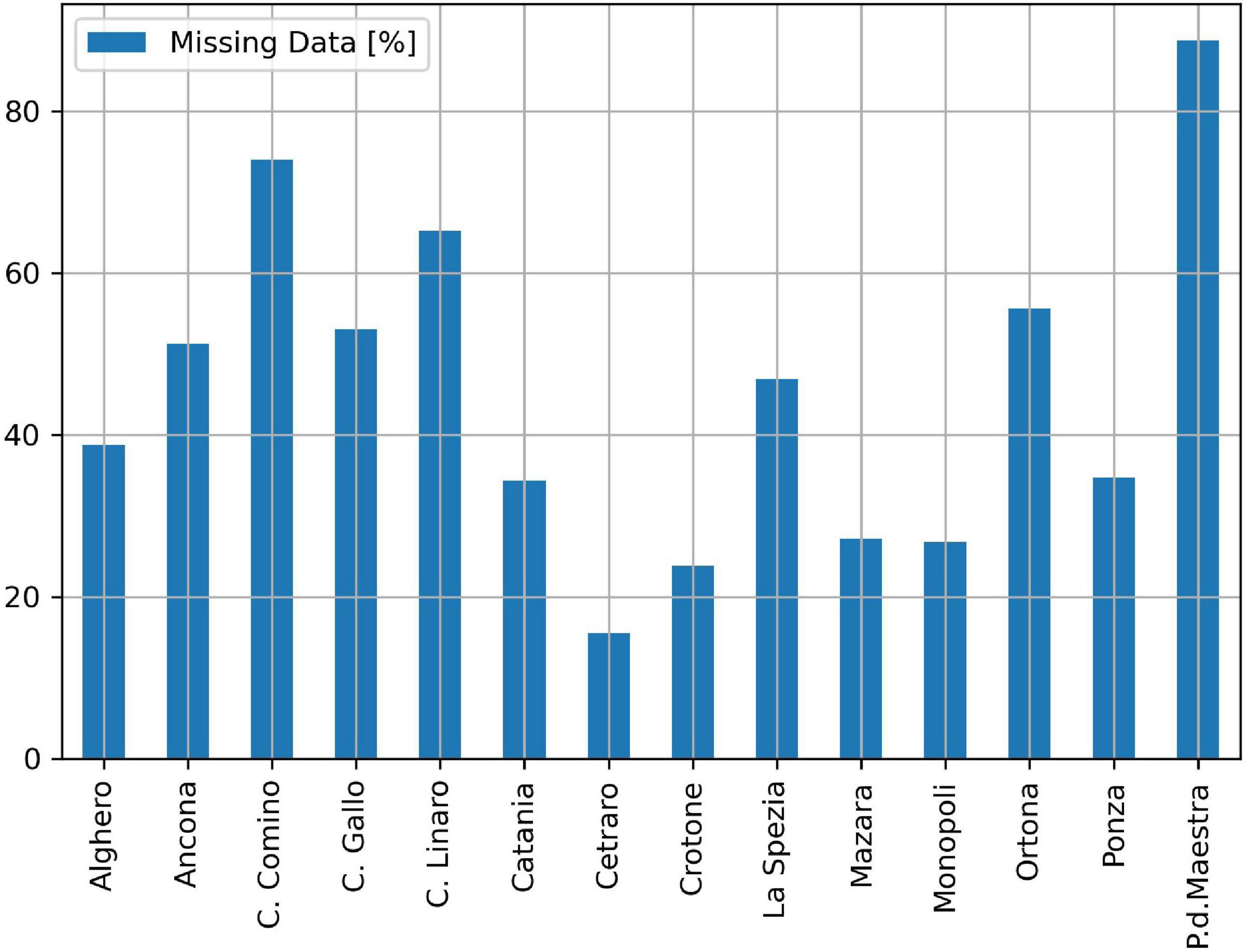
Figure 1. Missing data percentage of the 14 buoys of the Italian Data Buoy Network from 2002 to 2006. Source (Picone, 2009).

The maintenance issues are not specific of the Italian Data Buoy Network, and many works focus on missing data reconstruction using machine learning (ML) and data science methods. For example in Vieira et al. (2020), a method based on artificial neural networks is presented to fill the waves record gaps using offshore hindcast and wind information. In Jörges et al. (2021), a Long Short-Term Memory neural network was used to reconstruct the significant wave height from sea state time series, weather data of adjacent buoys, and bathymetric data. In Agrawal and Deo (2002), a first order “auto regressive integrated moving average” (ARIMA) model, e.g., see Nielsen (2019), was used and compared to a feed-forward neural-network for making sea wave predictions.

Besides data reconstruction, ML is key in many methods for oceanography (Lou et al., 2021). In fact, ML algorithms can find a mathematical model (called ML model) which produces the desired output when applied to a set of input data (called “training data”). The interesting part is the prediction, in which the ML model generates the correct outputs also when applied to new input data, distinct from the training data, coming from the same source. An important differentiation is between supervised learning and unsupervised learning. In the first case, the desired output is available for the training data, in the latter case, the desired output is not available. Supervised learning is more appropriate for missing data reconstruction because the desired outputs are typically available. For example, the desired output might be the sea wave data measured by a buoy whereas the input data comes from adjacent buoys, wind measurements, offshore hindcast, or, as we do in this work, micro-seismic data. During the regular operation, all data, including the desired output, are available and can be used for training. Instead, when data from the buoy are missing, the ML model will predict them from the input data. There are several ML algorithms able to make both regression (predict a continuous value, such as the significant wave height) and classification (predict a class, such as the degrees of the Douglas Sea scale). For example, there is whole family of algorithms, called artificial neural networks, inspired by natural neural networks. Other algorithms are the results of mathematical approaches, such as linear models, support vector machines, and decision trees. An introduction to machine learning is in Burkov (2019), while a more comprehensive exposition is in Géron (2019).

In this work, we will use micro-seismic data acquired from an onshore seismometer as input data. Actually, it is well known that sea waves are source of a micro-seismic signal which is detectable from onshore, even at many kilometers from the coast. Although this phenomenon has been discovered more than a century ago, the first geophysical model was presented in Longuet-Higgins (1950); more details are provided in the section “Background – From Micro-Seismic Signals to Sea Waves Parameters.” Improvements of this model have been proposed. For example, in Ardhuin et al. (2011, 2012) three different geophysical models were introduced for three different types of events. In other works, the relationship between the micro-seismic signal and the sea waves has been investigated with focus on specific locations (Barruol et al., 2006; Davy et al., 2016; Ferretti et al., 2018) and on specific events (Cutroneo et al., 2021). In Ferretti et al. (2013), an algorithm based on Markov chain Monte Carlo is used to determine the model parameters for a study conducted in the Ligurian coast (Italy). In Barruol et al. (2016), the authors evaluated the correlation between the polarization of the micro-seismic signal and the swell propagation direction. In Serafino et al. (2021), simultaneous measurements of a micro-seismic based system (called OS−IS) and those of a radar system were compared for the first time. In Cannata et al. (2020), a machine learning method (specifically, a random forest) was proposed to reconstruct the spatial distribution of sea wave height, as provided by hindcast maps of sea wave models, by using micro-seismic data from multiple seismic stations. In Moschella et al. (2020), a network of broadband seismic stations was used to investigate the micro-seismic signals from Ionian and Tyrrhenian Sea and, importantly, it was demonstrated that the signal detected by seismic stations closer to the sea contain more information concerning the sea state than the others.

As demonstrated in Iafolla et al. (2015), systems based on micro-seismic measurements outperform the systems based on moored buoys in terms of reliability and sustainability. Consequently in this work, we propose a measuring system consisting of a moored buoy, a micro-seismic measuring station, and a supervised machine learning algorithm to provide accurate sea wave measurements (specifically, significant waves height H_S, peak period T_p, and mean period T_m) continuously and reliably. This measuring system will typically provide the measurements from the buoy, which we will use as the desired output for the training data. Instead, the micro-seismic data are the input data, processed by the machine learning algorithms to reconstruct (i.e., “predict” in ML jargon) the sea wave data and fill the gaps due to the failures of the buoy. Therefore, the proposed system features the accuracy of the buoys and the reliability of the micro-seismic method overcoming the limitations of the two methods taken separately. In this work, we present the methods to preprocess the data, develop the ML models, and evaluate their accuracy. As a case of study, we will use the data recorded simultaneously by a buoy and a micro-seismic based system to validate the proposed methods and to assess their accuracy.

Background – From Micro-Seismic Signals to Sea Waves Parameters

In this section, we introduce a simple model, based on the Longuet-Higgins’s one, to derive the sea waves parameters from the micro-seismic signals. This model provides basic notions and it was inspirational to develop the ML methods. Furthermore in this work, it was used as a benchmark for comparisons.

Longuet–Higgins showed that a peak of the micro-seismic spectrum is related to sea waves traveling in opposite direction (e.g., waves generated by coastal reflection) with similar frequencies. A peculiarity is that the peak of the micro-seismic spectrum has doubled frequency compared to that of the sea waves. Another phenomenon, with lower seismic energy and same frequencies as the sea waves, originates by the interaction of the waves with a sloping bottom. A recent review and detailed description of these phenomena are given in Ardhuin et al. (2019). Considering the Longuet-Higgins phenomenon, a simple mathematical equation to calculate the significant wave height H_S from the micro-seismic power spectral density S(f) (with f being the frequency) is the following (Bromirski et al., 1999).

$H_S=\mathrm{\alpha }\cdot \sqrt{{\int }_{f_{min}}^{f_{max}}S\left(f\right)\cdot \mathit{d}f}+\mathrm{\beta }(1)$

In the previous equation, α and β are parameters of the model. The limits of integration f_max and f_min are also parameters and define a bandwidth that must contain all the micro-seismic signal generated by the sea waves. However, this bandwidth should not be too large, in order to avoid extraneous micro-seismic contributions that would worsen the accuracy of the evaluation of H_S. To calculate T_m and T_p, one can simply use S(f) in place of the sea wave power spectral density. However, we recall that the frequency of the micro-seismic signal is doubled compared to that of the sea waves. Therefore, T_p is 2/f_p (with f_p being the peak frequency of S(f)) and T_m is defined by the following mathematical formula (Krogstad et al., 1999).

$T_m=2\cdot \frac{\sqrt{{\int }_{f_{min}}^{f_{max}}S\left(f\right)\cdot \mathit{d}f}}{\sqrt{{\int }_{f_{min}}^{f_{max}}f\cdot S\left(f\right)\cdot \mathit{d}f}}(2)$

Materials and Methods

Measuring Systems

In this work, we used data collected in 2014 by a sea wave monitoring system, called OS−IS (Ocean Seismic -- Integrated Solution), based on the micro-seismic method and data by the buoy of the Italian Data Buoy Network moored in proximity of La Spezia. The latter data are publicly available on the European Marine Observation and Data Network (EMODnet)² and a detailed description of the Italian Data Buoy Network is in Bencivenga et al. (2012). The buoy ISPRA-La Spezia was moored at latitude 43°55′45.00″N and longitude 9°49′40.00″E (see Figure 2). At about 16 km (green line), the OS−IS station was installed in the basement of Villa Pezzino, the INGV (National Institute for Geophyisics and Volcanology) labs of Porto Venere (La Spezia), at latitude 44°4′24.19″N and longitude 9°50′22.84″E.

FIGURE 2

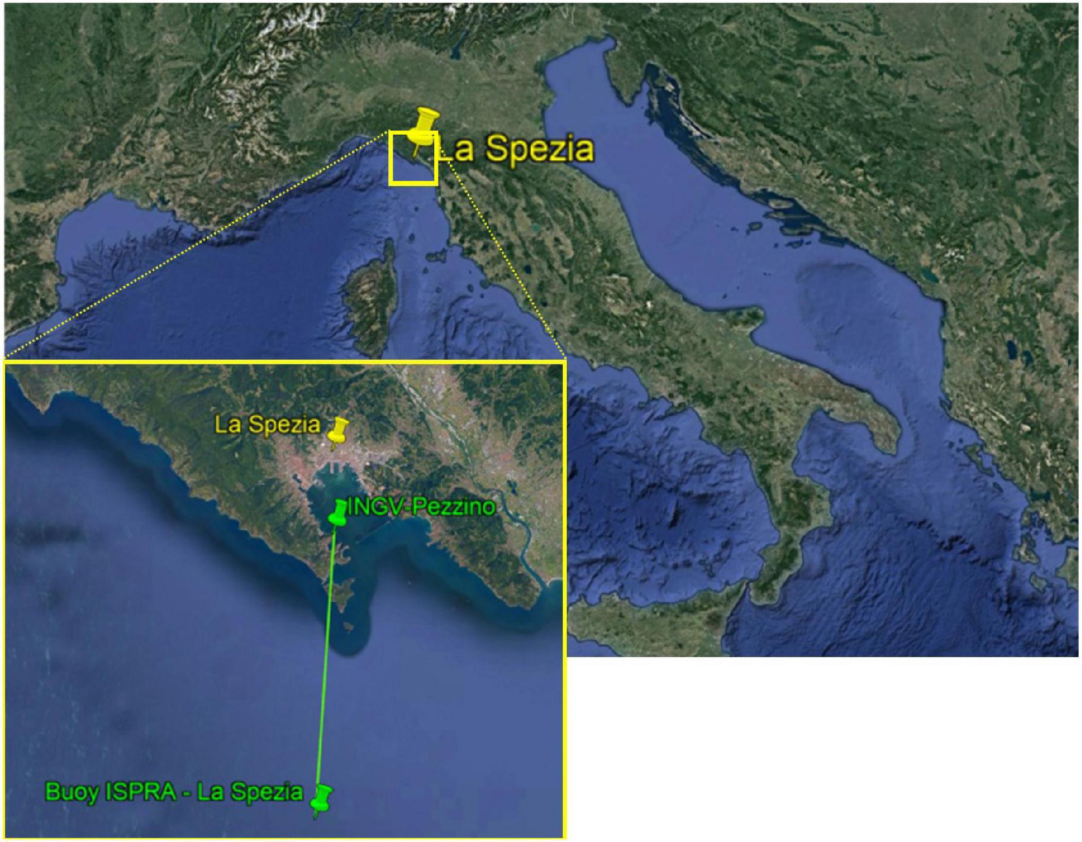
Figure 2. Locations of La Spezia city (yellow marker), OS-IS station (INGV-Pezzino, green marker), and buoy ISPRA-La Spezia (green marker). The distance, indicated by the green line, between OS-IS and the buoy is about 16 km.

The OS−IS station at INGV-Pezzino was installed in December 2013 in the framework of a project called Wind, Ports, and Sea (Bonino et al., 2015) funded by the European Cross-border Programme “Italy–France Maritime 2007–2013.” A detailed description of OS−IS is provided in Iafolla et al. (2014, 2015), Carmisciano et al. (2016) and its simplified schematic is shown in Figure 3. The core is the high-sensitivity three-axial accelerometer developed by AGI srl (Figure 4). Its background noise level is lower than 10^–7 m/s²/√Hz in the bandwidth of interest for measuring the micro-seismic signal generated by the sea waves (from ∼4.10^–2 to ∼1 Hz). The sampling rate of the accelerometer was set to 10 Hz, which is about 10 times bigger than the highest frequency of interest. Although all three components (x, y, and z) of the acceleration were available, in this work, we used only the vertical component, aligned to the local gravity.

FIGURE 3

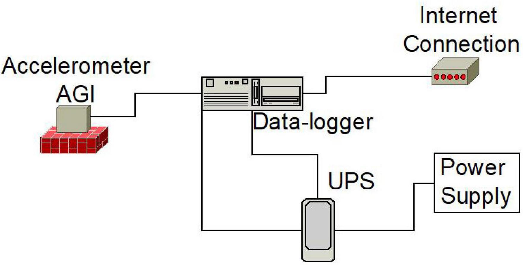
Figure 3. Simplified schematic of an OS–IS station. The UPS (Uninterruptible Power Supply) improves the reliability of the system. All instrumentation is installed indoor, sheltered from the environment (rain, humidity, dust, etc.). One OS–IS station might also include a weather station and a GPS receiver for weather monitoring and precise timing.

FIGURE 4

Figure 4. Picture of a three-axis accelerometer by AGI srl. The three gray elements are transducers for measuring the x, y, and z components of the acceleration. Typically, the accelerometer is closed to protect the transducers and the acquisition electronics.

The measurements from the accelerometer were transmitted, through the internet, to a server for data storage and processing. Further descriptions regarding the computing system are reported in the section “Introduction” of Supplementary Material of this manuscript.

Graphical Tools and Validation Metrics for Data Analysis

In this work, data analysis was key for two main tasks. The first was to explore data, identify anomalies, and, consequently, remove noisy records. The second was to validate the ML models and assess their performance. The validation is done by comparing two datasets: the predicted values and the desired values. For example, we compared the H_s values predicted by ML models and the H_s values measured by the buoy.

Performing the former tasks require several tools, both graphical and numerical. We used well-known graphical tools, such as time plots, scatter plots, and histograms, as well as less used (at least in -sea wave to micro-seismic- data analysis) tools such as empirical cumulative distribution function (ECDF) plots and hexagonal binning plots.

In ECDF plots (Downey, 2014), the value of the ECDF (y-axis) at any specified point x₀ of the x−axis is the fraction of observations of the variable× that are smaller than or equal to x₀. In formula, ECDF(x₀) = P(x≤x₀), where P(x≤x₀) is the probability that x≤x₀. ECDFs are useful for comparing sea wave distributions (Krogstad et al., 1999) because they smooth out random variations which, instead, are typical in histograms. Furthermore, synchronization of the records is not necessary, as with time plots, because the timing is lost in ECDFs.

Hexagonal binning plots are an alternative to the more common scatter plots to show and verify the relationship between two variables (Bruce et al., 2020). The records are grouped into hexagonal bins whose color indicates the number of records in that bin. The hexagonal binning plots are ideal to display large datasets that would appear as a monolithic cloud of points in conventional scatter plots. To make hexagonal binning plots, we used the hexbin function of the Matplotlib library of Python.

Other common methods for comparing two datasets are the validation metrics such as RMSE (Root Mean Squared Error), MAE (Mean Absolute Error), and Pearson correlation coefficient (Géron, 2019; Bruce et al., 2020). To compute them, we used the functions mean_squared_error, mean_absolute_error (from sklearn.metrics library of Python) and corrcoef (from numpy library).

Data Pre-processing and Cleaning

Exploratory Data Analysis

Exploratory data analysis (EDA) is a process for gaining an insight into a dataset (Downey, 2014). A golden rule in ML is to always perform an EDA before preparing the data and feeding them into a ML algorithm. For example in this study, it is relevant to know how the values of H_s, T_p, and T_m are distributed and if there is any relationship between them. The section “Background – From Micro-Seismic Signals to Sea Waves Parameters” of the Supplementary Material reports the results of an EDA conducted on the dataset used in this study.

Data Augmentation

The amount and the quality of the training data is important for successfully training ML algorithms. In other words, a large dataset well representing the population of possible inputs is desirable. Sometimes, new training data can be generated from the available ones, this is called “data augmentation” in ML jargon. For example, it might be sufficient to flip one image about its central axis to obtain a new sample image for training. However, the new sample should not be too much alike the original one, otherwise it will not determine any improvement of the training.

In our work, the size of the dataset was limited by the sampling period of the buoy, which was 30 min. To increase this size, we interpolated the buoy data to a sampling period of 10 min. To do so, we used the interpolate method of the Pandas library of Python with the interpolation parameter set to “quadratic.” We did not further decrease the sampling period to avoid feeding the ML algorithms with samples too much alike each other. For example, records of the sea wave parameters are displayed in the time plots of Figures 5A–C. In such short timing, the variations are already quite small because of the inertia of the sea state. Consequently, further interpolation would not determine any improvement of the training because the newly generated records would be almost identical to the existing ones.

FIGURE 5

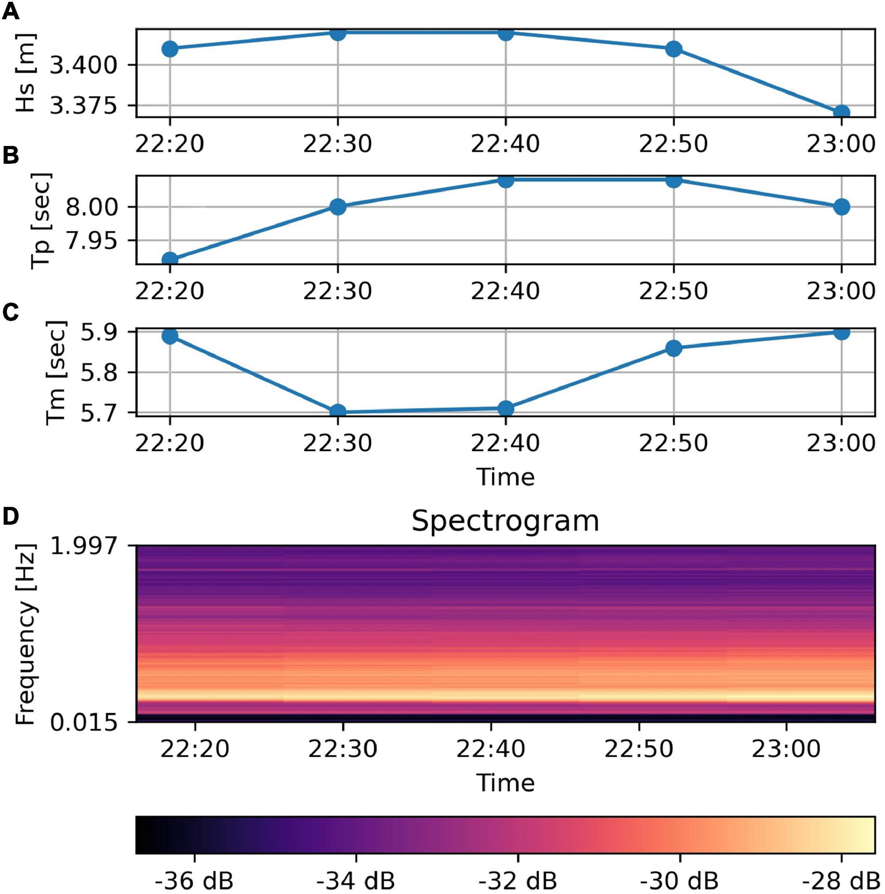
Figure 5. The time plots (A–C) show five buoy records from 22:20 to 23:00 on the February 5, 2014. In (D) is shown the spectrogram of the micro-seismic signal, i.e., the five columns represent the five PSDs corresponding to the timings indicated by the labels on the x axis.

Feature Engineering

Data pre-processing is called “feature engineering” in ML jargon, where the features are the input variables of the algorithm: for example, if the input is an array, each of its elements is a feature. In other words, feature engineering defines the shape of the ML algorithm input and impacts significantly its performance (e.g., the accuracy). Inspired by the model introduced in the section “Background – From Micro-Seismic Signals to Sea Waves Parameters” and timeseries forecasting methods (Nielsen, 2019), we defined and tested two methods to engineer the features, i.e., to pre-process the micro-seismic data. Both these methods use the power spectral density (PSD) of the micro-seismic signal, like that shown in Figure 6. Details on the method to compute the PSD are provided in the section “Materials and Methods” of Supplementary Material.

FIGURE 6

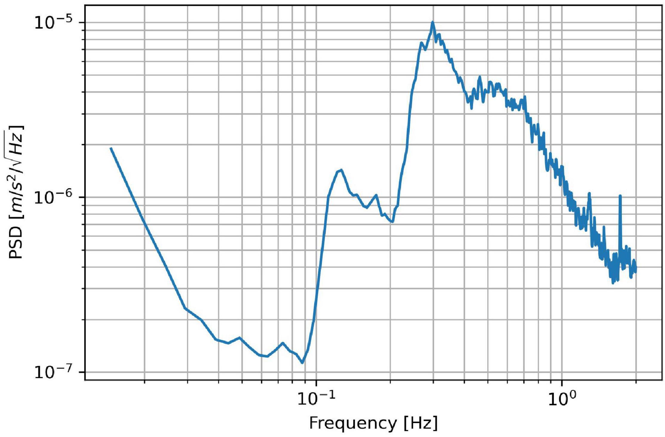
Figure 6. Power spectral density (PSD) of the micro-seismic signal recorded on the February 5, 2014 at 23:00. The corresponding sea waves parameters from the buoy were: H_s = 3.37 m; T_p = 8.00 s; and T_m = 5.90 s.

We defined the first feature engineering method inspired by Equations 1, 2, which contain the micro-seismic spectrum S(f). This method merely consists in using the PSD as ML algorithm input.

We defined the second feature engineering method inspired by the analysis of the properties (stationarity, autocorrelation, partial-autocorrelation, etc.) of the timeseries H_s, T_p, and T_m and, specifically, by the possibility to predict their present value from their past values (Nielsen, 2019). For example, Figure 7 shows that an ARIMA(3,1,5) model can forecast H_s using its past five values. This suggests that past H_s values carry useful information to evaluate the present value. Similarly, we supposed that the past records of the PSD might carry useful information to evaluate the present sea state. To leverage this, we used a spectrogram, i.e., an image combining the last five PSDs like that shown in Figure 5D, as ML algorithm input. Similar spectrograms with more than five PSDs could be used, however they require more memory and computational power. More details on the computation of the spectrogram are provided in the section “Materials and Methods” of the Supplementary Material.

FIGURE 7

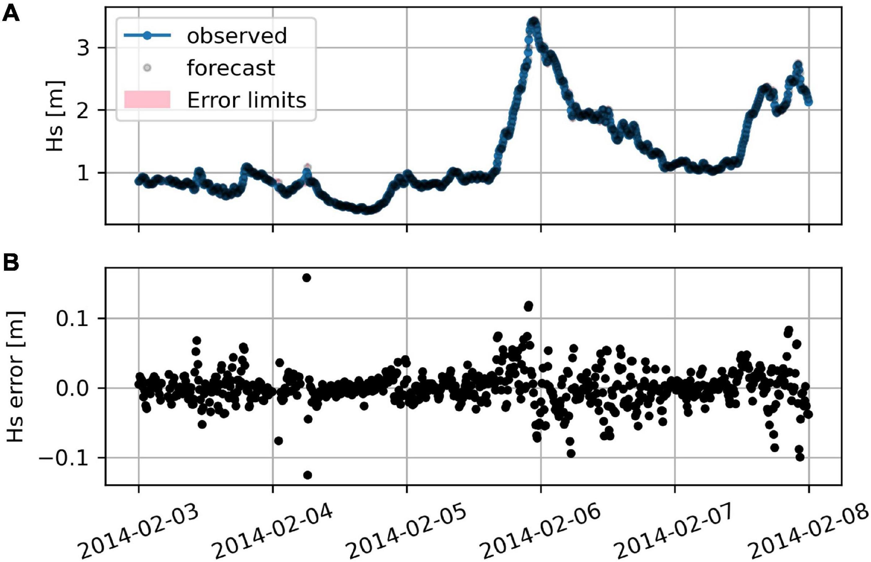
Figure 7. (A) H_s observed by the buoy and forecasted with an ARIMA(3,1,5) model. Each forecast is evaluated using the past observed values. The error limits are too small to be visible on this scale. (B) Deviation of the forecasted values from the observed ones.

Summarizing, the first feature engineering method consists in feeding the ML algorithm with the present PSD of the seismic signal; the second in feeding it with the last five PSDs (i.e., the spectrogram).

Data Cleaning

Data cleaning is aimed at achieving optimal results in ML and at checking the quality of the records during the operational use. Given the big amount of data and the real-time applications, it is also important to automatize the cleaning and the quality checking.

Data from the buoy were already classified with a quality check label (“good value,” “bad value,” etc.). We merely discarded all those samples whose label was not “good value.” Other records were dropped because the corresponding micro-seismic data were not available. The number of available and missing records is reported in Supplementary Table 1. In addition, we picked just the variables of our interest (i.e., timestamp, H_s, T_p, T_m, and swell direction) and dropped all other variables (e.g., temperature of the water, intensity of the wind).

To perform micro-seismic data cleaning, it was useful to compute a timeseries I_PSD(t), or simply I_PSD, of the mean values of the elements of the PSDs. For example, I_PSD(5^th February 2014 at 23:00) is the mean value of the points shown in the plot of Figure 6. For convenience, we standardized I_PSD(t) by subtracting its mean value and dividing by its standard deviation. Furthermore, it was useful to compute the timeseries, diff(I_PSD), of the variations of each record of I_PSD with respect to the recent previous ones. To do so, we used a rolling window (4 h wide) technique over I_PSD; i.e., diff(I_PSD) is the difference between the value of last point and the mean value within the window.

Using I_PSD(t) and diff(I_PSD) we could identify noisy data caused by micro-seismic disturbances. Most common examples of the latter are earthquakes and human activities, such as people walking next to the accelerometer. These disturbances might last for several minutes and they might affect several consecutive input samples (i.e., PSD records). This is visible in the time plots of I_PSD, such that in Figure 8A. Bunches of points, highlighted in red, are clearly displaced away from the others, indicating an anomaly. Sometimes, these anomalies are very high and setting a threshold over I_PSD is sufficient to spot them automatically. An example is the bunch of points recorded on the 24th of May. However, their values are often lower than peaks due to the sea waves. For example, the bunch of red points recorded on the 9th of May are clearly anomalies because they do not have correspondence with the H_s measured by the buoy (Figure 8C). Still, their I_PSD values are lower than the peak on the 13th, which is due to sea waves. To automatically identify these points, we used diff(I_PSD), shown in Figure 8B, where these points emerge from the rest.

FIGURE 8

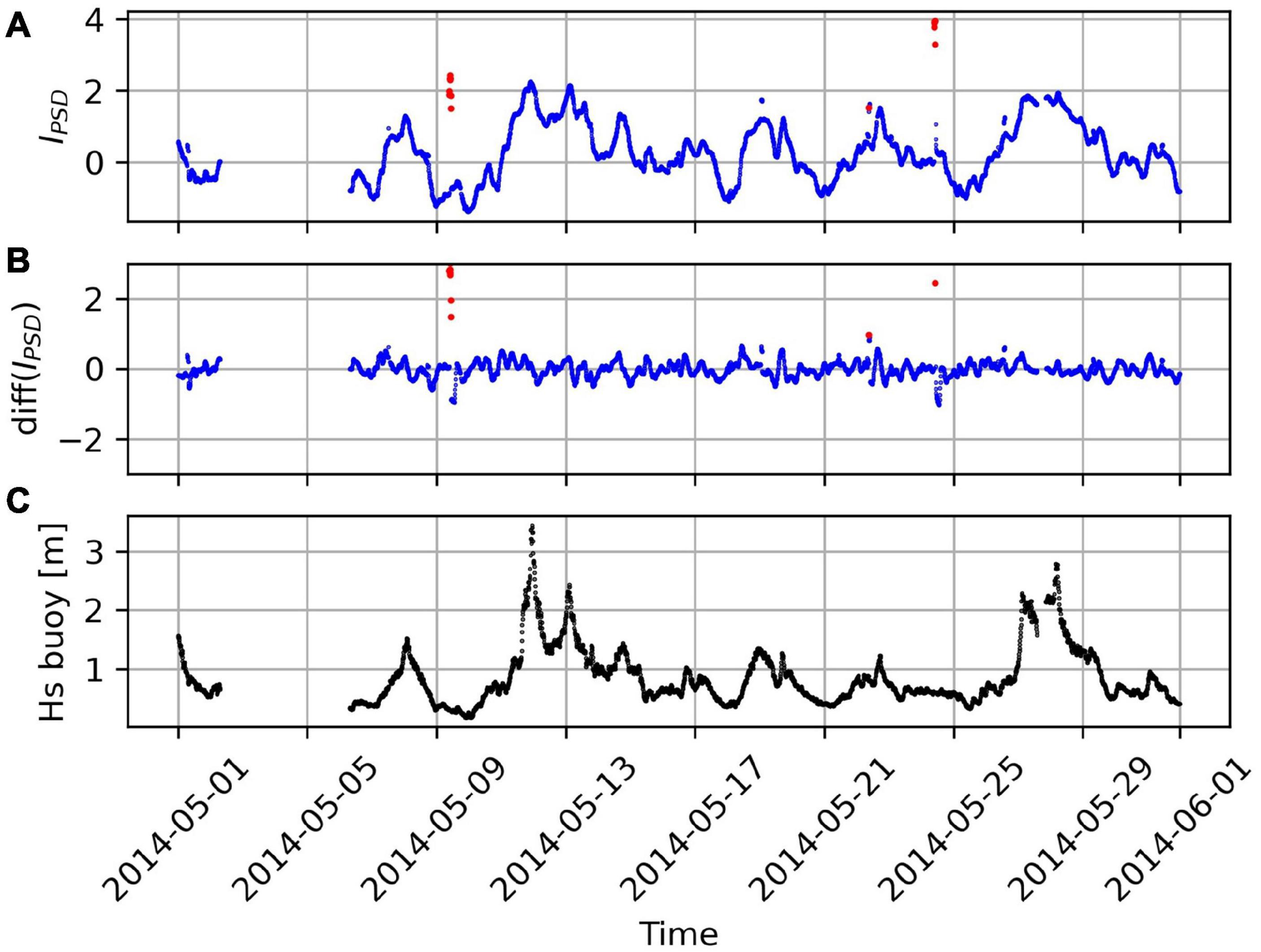
Figure 8. Time plots of (A) I_PSD, (B) diff(I_PSD) (as defined in the section “Data Pre-processing and Cleaning”), and (C) H_s. Anomalies are in red.

To automatically identify and discard anomalies, we made the scatter plot of I_PSD vs. diff(I_PSD) as shown in Figure 9. Most of the records are close to the center (0,0), as also visible from the side and top histograms, whereas the anomalies are far away. Consequently, we defined an ellipse (shown in red), inside which all good records are expected to be. The anomalies, colored in orange, are outside the ellipse and, consequently, easy to discard. Defining the size and the position of the ellipse is trade-off: when it is too small, some good records might be wrongly discarded; when it is too large, some anomalies might not be identified as such. In our case, we defined the I_PSD axis length equal to 6 and the diff(I_PSD) axis length equal to 2.2.

FIGURE 9

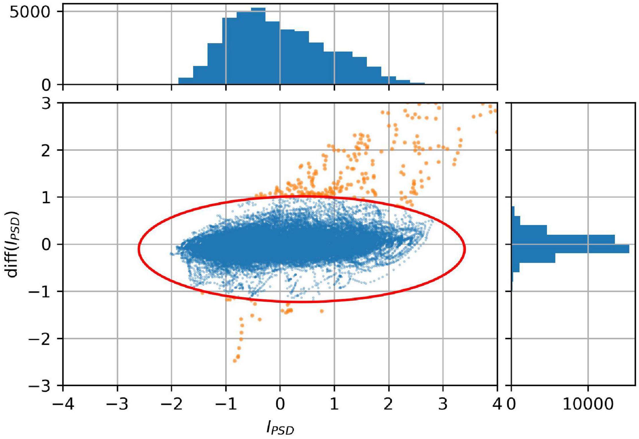
Figure 9. Scatter plot and corresponding histograms of I_PSD vs. diff(I_PSD). All points outside the ellipse, colored in orange, are identified as anomalies.

Machine Learning Algorithms and Models Validation

Machine Learning Algorithms

The ML algorithms able to predict the sea state with the highest accuracy were ensembles of decision trees (bagging, boosting, and random forests) and convolutional neural networks (a special case of deep learning algorithms).

A decision tree (DT) (Géron, 2019; Bruce et al., 2020) is a process that sequentially examines, one per time, the features of an input sample assigning it to an output value. However, only a finite number of possible output values is defined during the training, consequently, the output is discrete.

Ensemble methods overcome the limit of the discrete output and improves the accuracy of the DTs. In general, an ensemble is a group of predictors, e.g., a DT, making predictions on the same input sample. The output of the ensemble is an aggregation, e.g., the average, of all predictions. There are several ensemble methods; we used bagging, boosting, and random forest (Random F.), which are among the most commonly used (Géron, 2019). We implemented the ensembles using the dedicated functions of the Scikit Learn library of Python and we fed them with the PSDs defined in the section “Data Pre-processing and Cleaning.” The most important parameters of the ensemble methods are the max depth of the DTs and the number of predictors (called n_estimators in Scikit Learn). We used max depth equal to 7 and number of predictors equal to 15 or 20.

Finally, we trained and tested convolutional neural networks (CNNs), which were developed for processing images such as the spectrograms described in the section “Data Pre-processing and Cleaning.” For example, CNNs are famous for being able to classify pictures of dogs, cats, or other objects. Adjusting their output layer, they can also make regression as needed for the sea wave variables. A CNN consists of several layers of different types that are stacked and set accordingly to the task (Géron, 2019). Very complex tasks usually require high number of layers, large training datasets, and the training takes very long time (or very large computational power). The configurations we tested in this work are reported in Supplementary Table 2.

Machine Learning Models Validation

After a ML algorithm has been trained using training data, it provides a ML model. This can predict the output given only the input data; however, its performance should be assessed before using it. To make this assessment, the graphical methods and the metrics introduced in the section “Graphical Tools and Validation Metrics for Data Analysis” can be used to compare the outputs of the model with the desired outputs. This assessment is called validation and it is performed over a validation dataset that must contain also the desired outputs. However, a ML algorithm might be able to memorize (this is called overfitting) the training data without being able to generalize over new input data. Therefore, keeping the training data separated from the validation data is key to validate correctly the ML model even when it is overfitting. One method is based on holding out a validation subset and training the ML algorithm by using the rest of the dataset. However, the validation results might depend on the chosen validation subset. To overcome this issue, we used a method called cross-validation (Géron, 2019; Bruce et al., 2020); the idea is to split the full dataset in subsets, e.g., 12 (see Figure 10). The ML algorithm is then trained 12 times, each time holding out a different subset and using it only for validation. Merging the results, we can obtain validation estimates over the full dataset.

FIGURE 10

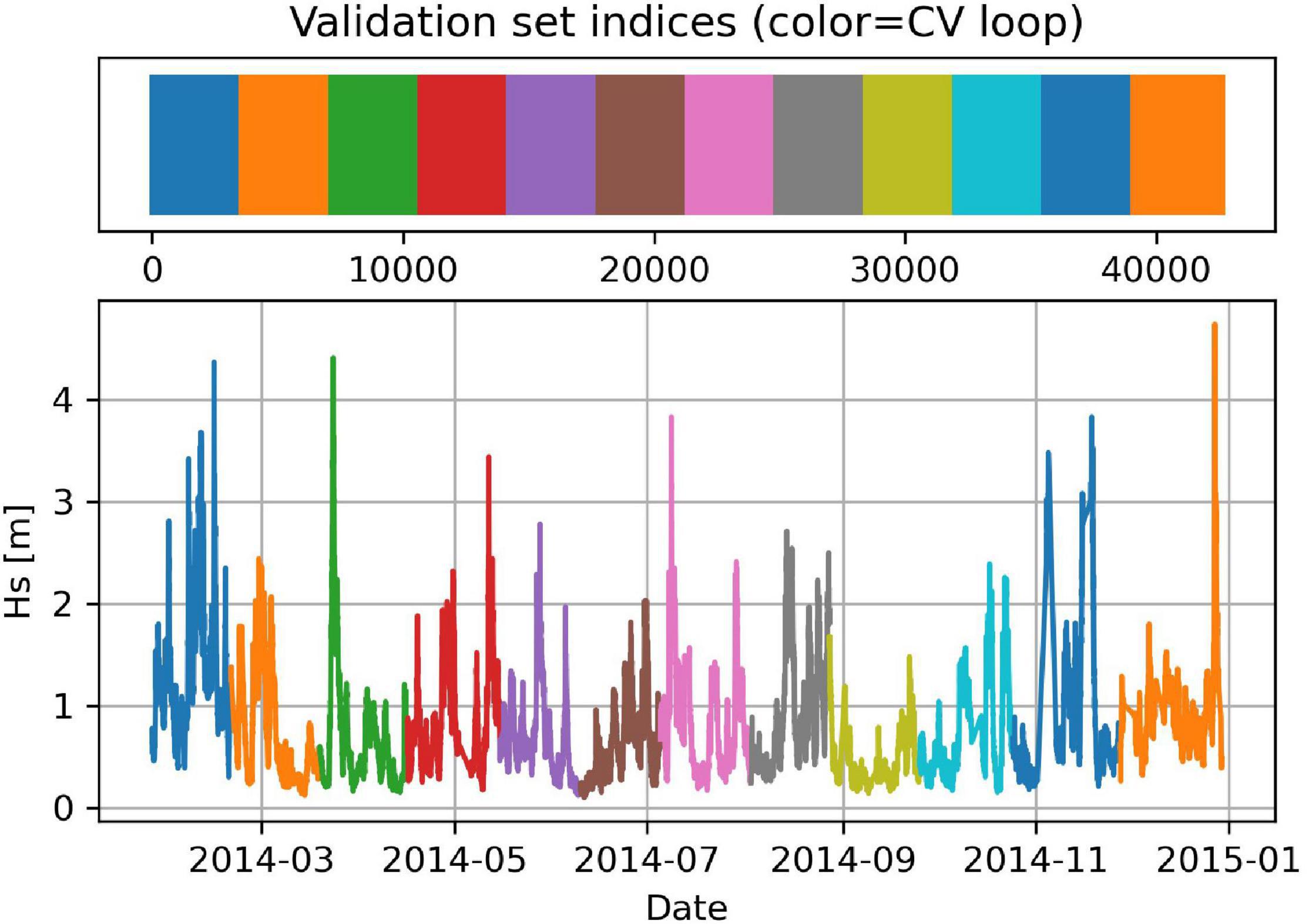
Figure 10. In cross-validation, the full dataset is split in subsets (e.g.,12) of the same size. In this figure, different colors indicate different validation subsets.

The bootstrap method (Bruce et al., 2020) can be used to assess the confidence intervals of the validation metrics. In this work, we used a similar method that allows us to inspect the performance of the ML model over the time. The idea is to estimate the validation metrics over multiple (e.g., 50) consecutive time intervals. Specifically, first we divided the validation dataset in 50 consecutive subsets, then we estimated the validation metrics of each subset to obtain a timeseries. This can be plotted to see how the ML model behaved over time and its ECDF can be used to easily assess the confidence intervals. Examples are shown in the section “Results,” Figure 11.

FIGURE 11

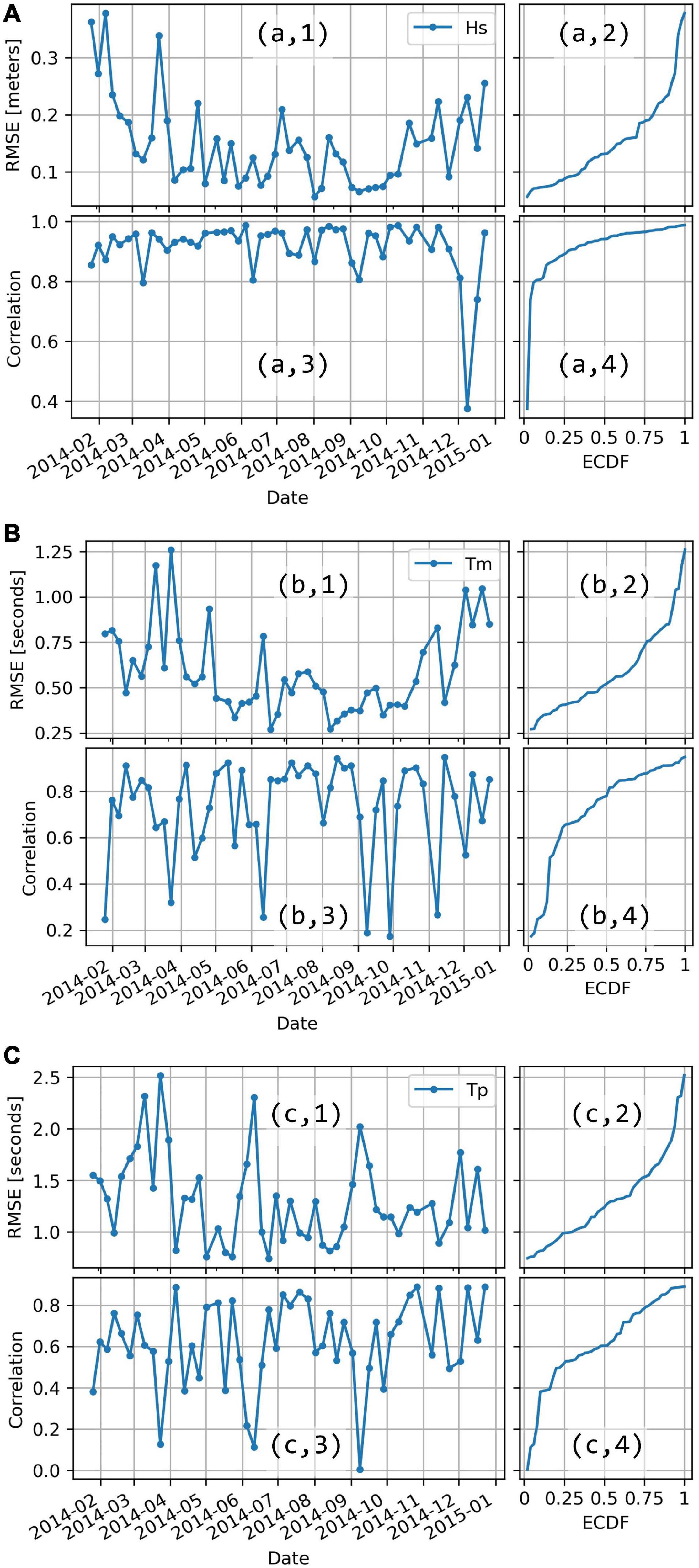
Figure 11. Validation metrics (RMSE and correlation) of the Random Forest ML model (20 predictors) computed over 50 different time spans. (A–C) labels are referred to Hs, Tm, and Tp, respectively. 1 and 3 are the time plots of RMSE and correlation respectively, whereas 2 and 4 are their ECDF plots.

Results

The dataset used for training and validating the ML models was made of 42603 simultaneous records, whereas 9957 records were not available or discarded during the data cleaning (see Supplementary Table 1, for more details).

The validation metrics of the best performing ML models and those of the conventional model introduced in the section “Background – From Micro-Seismic Signals to Sea Waves Parameters” (indicated as OS−IS Model) are reported in Table 1, 2. The OS−IS model is a good benchmark to assess the improvement achieved with the ML method because its performance was assessed using the same instrumentation and the same data. Rarely the OS−IS model performed better than the others, except for the MAE of T_p. The reason is that the OS-IS model was designed to provide measures of T_p only if H_s was larger than 1 m, when the signal to noise ratio was higher. To make a fair comparison, the last columns of Table 1, 2 report the validation metrics of a ML model (Boosting 20 pred.) trained and validated using the same dataset as for the OS-IS model (i.e., featuring H_s>1 m). As expected, its the validation metrics for T_p and T_m outperform those of the others, including those of the OS−IS model. This also highlights that the validation metrics depend on H_s and, more in general, on the training/validation data.

TABLE 1

Table 1. Performance of the ML models trained and validated over the data from 2014.

TABLE 2

Table 2. Performance of the ML models trained over the data from 2014 and validated over the data from November to December 2014 (6229 records).

Comparing the ML models reported in Table 1, we notice that the difference between them is rather small, anyway, Random F. performed slightly better than the others on all metrics.

In Figure 11, the validation metrics (RMSE and correlation) are estimated 50 times over consecutive time intervals of about 1 week each (see “ML models validation” in the section “Machine Learning Algorithms and Models Validation”). Notice the high variability of the estimates. On the right side of each time plot, the ECDF plots are shown and are useful to assess the confidence intervals. For example, in Figure 11 (a, 2) the median (ECDF = 0.5) of the RMSE estimates is ∼0.13 m and 90% (ECDF = 0.9) of the RMSE estimates are smaller than ∼0.25 m. Similarly, only 10% (ECDF = 0.1) of correlation estimates are smaller than ∼0.8.

Table 2 reports the validation metrics for a subset comprising only data from November to December 2014 (6229 records). Compared to the estimations in Table 1, the validation metrics are similar for H_s and T_p, but they are slightly worse for T_m. The same validation data are shown in Figure 12 and Supplementary Figures 5, 6. Specifically in these figures, the predicted values of H_s, T_p, and T_m are compared to the desired outputs provided by the buoy. Inspecting these figures provides us with more insights than the validation metrics. For example, we notice that the absolute errors of H_s (Figure 12B), might be bigger than 1 meter (e.g., see the orange ellipse), but often this is due to a time-lag between the buoy measurements and predicted values. In fact, in subplot (a) we do not see a deviation bigger than 1 m between the buoy and predicted data (see the orange circle). Consequently, the MAE and the RMSE of H_s reported in the tables might be overestimated. On the other hand, histograms and ECDF plots do not suffer from the time-lag issue. For example, Figures 12C,D show a good agreement between buoy and predicted data. On the opposite, histograms and ECDF plots (c) and (d) of T_p and T_m in Supplementary Figures 5, 6 do not overlap as nicely as with H_s. This indicates that assessing accurately T_p and T_m is slightly more complex than assessing the H_s.

FIGURE 12

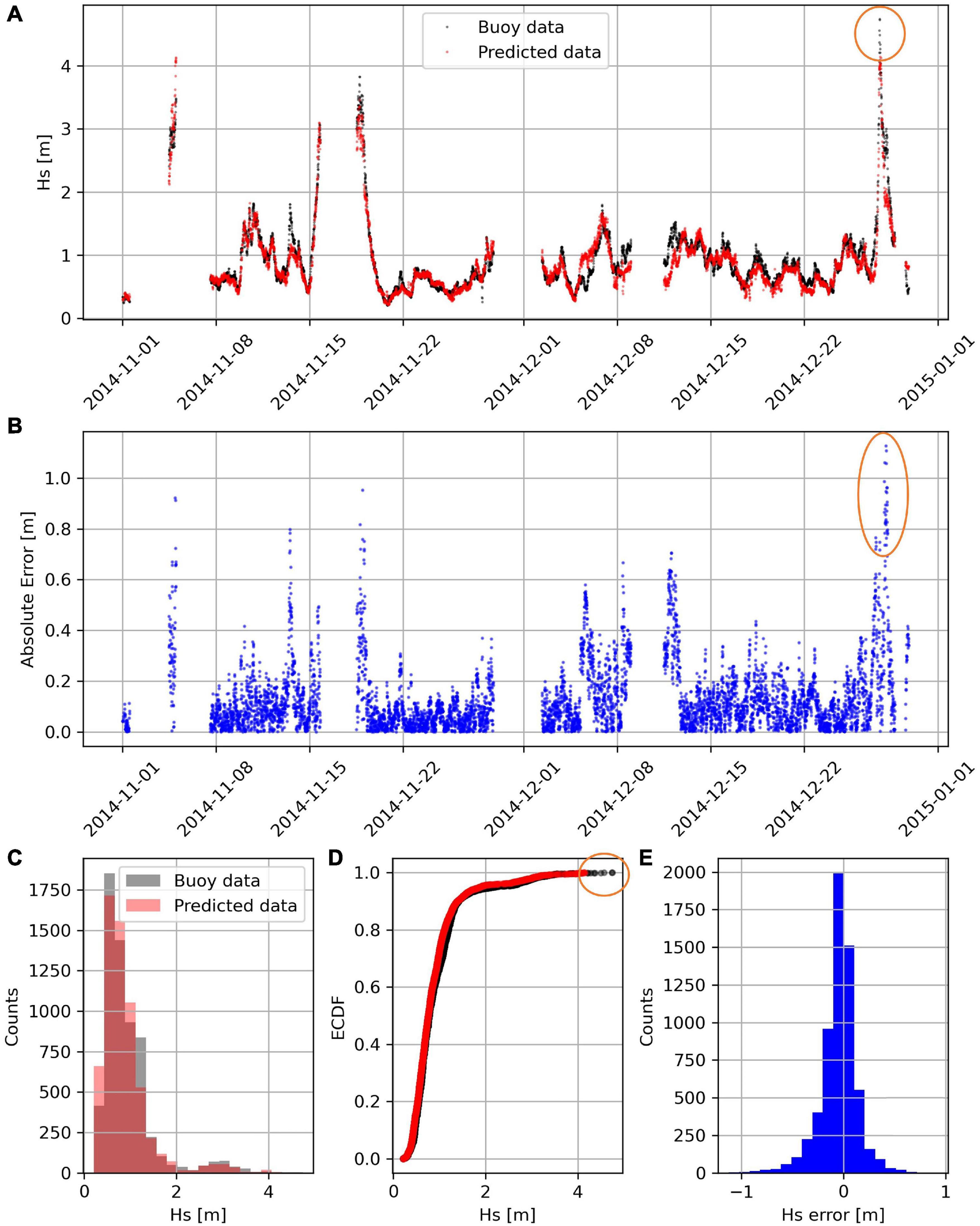
Figure 12. Significant wave height (H_s) measured by the buoy (in black) and predicted by the Random Forest model (20 predictors) (in red) displayed in the time plot (A), the histogram (C), and the ECDF plot (D). The deviation between the two-time series is displayed (in blue) in the time plot (B), and the histogram (E).

Inspecting the errors histograms [subplots (e)] is a good way to evaluate if the ML model is introducing a systematic error. In fact, this would skew the histogram or displace its center away from zero; however, such effects were not detected in our case.

Finally, Figure 13 shows the hexagonal binning plots of the predicted values vs. the desired values from the full dataset. Each plot also shows a black straight line along which the points are expected to align in the ideal case. We notice that for H_s [subplot (a)], the points are mainly concentrated next to the black line for values smaller than 2 m whereas they are more spread for bigger values. However, the hue also indicates that values bigger than 2 m are much less frequent; consequently, the ML algorithm is less exposed to those values during the training, leading to worse accuracy. The spreading of T_m and T_p, subplots (b) and (c), is not significantly larger for bigger values. However, we noticed that the points of T_p [subplot (c)] do not distribute symmetrically about the black straight line, particularly for values between 2 and 4 s (inside the yellow circle). Most likely, this is driven by those records whose H_s < 1 m. In fact, when the signal to noise ratio is lower (i.e., H_s < 1 m), it is harder to identify the peak frequency (i.e., the peak period) than when the signal to noise ratio is higher (i.e., H_s>1 m). This agrees with the validation metrics reported in the last columns of Table 1, 2.

FIGURE 13

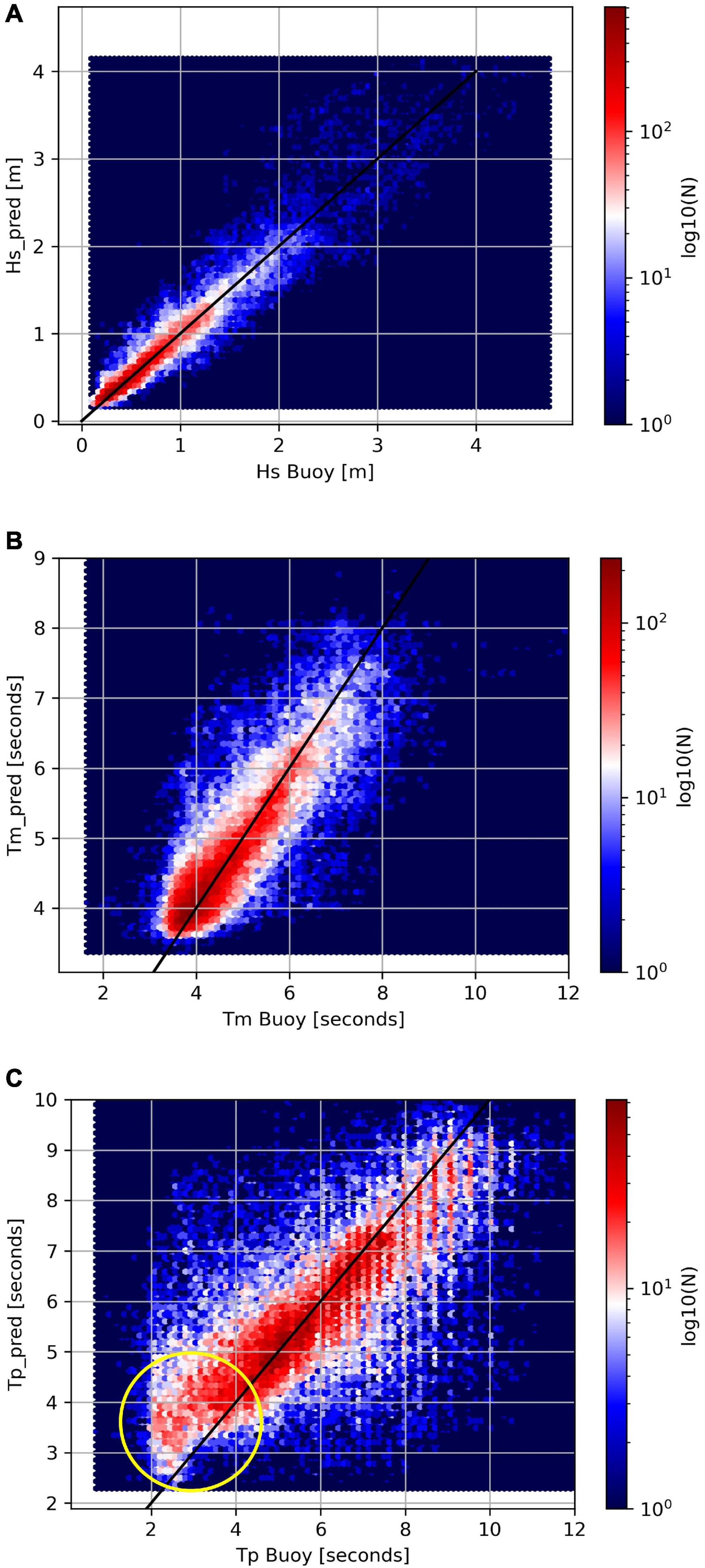
Figure 13. Hexagonal binning plots of the H_s (A), T_m (B), and T_p (C) values predicted by a Random Forest (20 predictors) model vs. those measured by the buoy. Validation data from 2014.

Discussion

The objective of this work has been to develop a sea wave monitoring system consisting of a moored buoy, a micro-seismic station, and a ML algorithm to automatically reconstruct missing buoy data using micro-seismic data. In this section, we discuss many aspects that differentiate our work from previous ones in the same field.

To begin, reconstructing missing buoy data using micro-seismic data is a novel aspect as, in previous works, other types of input data were used. For example, offshore hindcast and wind information were used in Vieira et al. (2020) and weather data of adjacent buoys and bathymetric data were used in Jörges et al. (2021). Moreover, many works were limited to short term (less than 48 h) predictions meaning that their models rely on recent observations of the buoy, e.g., (Agrawal and Deo, 2002). Instead, the proposed system can make predictions for any time after the last buoy observation keeping the same level of accuracy. This is key as buoy data gaps might be several weeks long.

As reported in the section “Introduction,” several previous works investigated the methods to retrieve sea wave data from micro-seismic data. A key aspect of the present work is the application of ML to automatically find the -micro-seismic to sea waves relationship- directly from data, with no need to develop and calibrate complicated geophysical models. Furthermore, the more training data are collected during the operations, the more accurately the ML model can perform. For example, by routinely training the ML algorithm as soon as new data is available, new types of events will be incorporated in the ML model with no need of manually tweaking its parameters, e.g., as in Cutroneo et al. (2021). Despite these many advantages, ML limits the investigation on the input-output relationship (i.e., on the geophysical phenomenon) because most of the ML algorithms are “black boxes.” Although this would be limiting in projects whose objective is to investigate the geophysical phenomenon, e.g., (Ardhuin et al., 2011), it is not relevant for missing data reconstruction.

Many aspects of the system were defined accordingly to the objective. For example, the micro-seismic station used for this work was specifically installed close to the shoreline and in front of the buoy of La Spezia (see Figure 2). As demonstrated in Moschella et al. (2020), this displacement of the instrumentation leads to more accurate buoy data reconstruction. In fact, undesired signals, such as those from remote seismic sources, are less relevant and the signal to noise ratio is higher than that of stations far away from the shoreline and the reference buoy. For example in Ferretti et al. (2013), the micro-seismic stations were from previous projects with different purposes (e.g., seismic monitoring) and, due to their locations, the interpretation of the signals was more complex.

Pursuing our objective, it was also important to use buoy data to train the ML algorithm and not weather model data, e.g., as done in Cannata et al. (2020). In fact, if the sea wave data from weather models were a ground truth, there would be no need to retrieve the same data from any monitoring system. On the opposite, sea wave monitoring data are critical to validate weather models and implement data ingestion techniques.

In the section “Materials and Methods,” we have gone through the main steps of the data processing; these are the typical steps of a ML project. Data cleaning is very important because ML algorithms are very sensitive to outliers and noisy data: the proposed method to clean the micro-seismic data is quite standard but still very effective; furthermore, it can be used to check the quality of the results during the monitoring operations. Despite the importance, data cleaning methods were seldom discussed in previous works. Feature engineering typically impacts the overall performance of ML models. We proposed two methods: one is based on using PSD arrays, the other on spectrograms; the latter was specifically meant for CNNs. Then, we introduced some ML algorithms and assessed their performance. Random forest was the best performing while CNNs did not shine as expected. Notice that the method to estimate and validate sea wave periods (T_p and T_m) from the micro-seismic data was discussed. This was often disregarded in previous works and the validation of waves period estimates was rarely presented. Still, the waves period is an important parameter to assess the energy and, consequently, the impact of the sea waves.

We have shown that the performance assessments, in particular the validation metrics, depend on the validation dataset. For example, the periods are better evaluated when H_s is bigger than 1 m; this should not be surprising because the signal to noise ratio is higher. To avoid wrong performance assessments, we proposed to use cross-validation, which is rarely used in projects related to the calculation of sea wave data from micro-seismic signals. Furthermore, we proposed a method to evaluate the confidence interval of the validation metrics using their ECDFs.

Our results for the accuracy on H_s estimates are comparable to those of other works. However, accuracy depends on many variables (e.g., validation dataset, measurement site, sea wave conditions, and time interval length) that make such comparisons meaningless. Consequently, the accuracy estimations should be used only to assess the ability of the system to reconstruct the missing buoy data.

It is worth to stress that the proposed system is an improvement of an existing technology for sea state monitoring, i.e., that of moored buoys. Accordingly, the micro-seismic system is not meant to operate as a standalone device. Therefore, the buoy is expected to continuously provide training data, particularly of sporadic events such as rare storm events; once these are incorporated in the training dataset, the ML algorithm will learn how to reconstruct them from the micro-seismic data. On the opposite, if the buoy is dismissed at some point in time, some new sporadic events might occur and the ML algorithm would not be able to reconstruct them accurately.

Finally, we stress the value of data science methods that are poorly and seldomly used in studies related to the evaluation of sea wave data from micro-seismic signals. Besides the ML methods, we have shown methods to compare timeseries and distributions. These are key when comparing and validating complex data such as sea wave measurements. For example, conventional scatter plots were often shown, where points formed a monolithic cloud hiding most of information. Instead of scatter plots, we proposed to use hexagonal binning plots. The validation metrics, such as RMSE, MAE, and correlation, were typically reported but, although very useful, they rarely tell the whole story. Instead, tools such as the ECDF plots were rarely used despite they are more informative than validation metrics.

Conclusion

In this work, we introduced a novel sea state monitoring system able to automatically reconstruct missing buoy data using micro-seismic data and machine learning. Specifically, we presented the methods to process the data, develop and train the ML algorithms, and assess their accuracy. As a case of study, we used the data collected in 2014 from a buoy of the Italian Data Buoy Network and a micro-seismic station (OS−IS). We demonstrated that many ML algorithms were able to reconstruct H_s, T_m, and T_p. However, the best performing was a Random Forest algorithm, whose root mean squared errors of H_s, T_m, and T_p were, respectively 0.17 m, 0.63, and 1.38 s. When H_s was bigger than 1 m, the accuracy of T_m and T_p improved to, respectively 0.57 and 0.97 s.

By collecting more data, particularly for rare storm events, and tweaking the ML algorithm architectures, we believe that the accuracy can further improve. Specifically, we believe that the full potential of the CNN and the spectrograms as input, was not fully exploited. To do it, spectrograms with larger time span should be used and the CNN models should be more complex (i.e., more parameters). However, this requires more computational power than that available for this work.

Data Availability Statement

The original contributions presented in the study are included in the article/Supplementary Material, the micro-seismic data are available upon request to the authors. Further inquires can be directed to the corresponding author.

Author Contributions

LI: conceptualization, methodology, software, validation, investigation, writing – original draft, writing – review and editing, and visualization. EF: validation, investigation, writing – review and editing, and supervision. MC: writing – review and editing, supervision, project administration, and funding acquisition. CC and VI: conceptualization, methodology, validation, investigation, writing – review and editing, supervision, project administration, and funding acquisition. All authors contributed to the article and approved the submitted version.

Funding

This research was funded by Assist in Gravitation and Instrumentation srl (AGI). The open access publication of this work was funded by Istituto Nazionale di Geofisica e Vulcanologia. The OS-IS station used in this work was financed by the European Regional Development Fund within the project Vento, Porti e Mare. The wave buoy data used in this publication were from ISPRA (Istituto Superiore per la Protezione e la Ricerca Ambientale, Italy) and made available by the EMODnet Physics project (www.emodnet-physics.eu/map, funded by the European Commission Directorate-General for Maritime Affairs and Fisheries).

Conflict of Interest

LI and EF are employed by AGI srl. AGI srl commercializes products and has filed a patent (still pending in January 2022) relevant to the system presented in this work.

The authors declare that the research was conducted in the absence of any commercial or financial relationships that could be construed as a potential conflict of interest.

Publisher’s Note

All claims expressed in this article are solely those of the authors and do not necessarily represent those of their affiliated organizations, or those of the publisher, the editors and the reviewers. Any product that may be evaluated in this article, or claim that may be made by its manufacturer, is not guaranteed or endorsed by the publisher.

Supplementary Material

The Supplementary Material for this article can be found online at: https://www.frontiersin.org/articles/10.3389/fmars.2022.798167/full#supplementary-material

Footnotes

1. ^ https://www.datawell.nl/Products/Buoys.aspx
2. ^ https://www.emodnet-physics.eu/map/platinfo/piroosplot.aspx?platformid=8712

References

Agrawal, J. D., and Deo, M. C. (2002). On-line wave prediction. Mar. Struct. 15, 57–74. doi: 10.1016/S0951-8339(01)00014-4

CrossRef Full Text | Google Scholar

Andrews, E., and Peach, L. (2019). “An evaluation of current and emerging in-situ ocean wave monitoring technology,” in Proceedings of the Australasian Coasts and Ports 2019 Conference: Future Directions From 40 [Degrees] S and Beyond, Hobart, 10-13 September 2019. Engineers Australia, Hobart, TAS.

Google Scholar

Aouf, L., Hauser, D., Chapron, B., Toffoli, A., Tourain, C., and Peureux, C. (2021). New directional wave satellite observations: towards improved wave forecasts and climate description in southern ocean. Geophys. Res. Lett. 48:1187. doi: 10.1029/2020GL091187

CrossRef Full Text | Google Scholar

Ardhuin, F., Balanche, A., Stutzmann, E., and Obrebski, M. (2012). From seismic noise to ocean wave parameters: general methods and validation: ocean wave parameters from seismic noise. J. Geophys. Res. Oceans 117:449. doi: 10.1029/2011JC007449

CrossRef Full Text | Google Scholar

Ardhuin, F., Stopa, J. E., Chapron, B., Collard, F., Husson, R., Jensen, R. E., et al. (2019). Observing Sea States. Front. Mar. Sci. 6:124. doi: 10.3389/fmars.2019.00124

CrossRef Full Text | Google Scholar

Ardhuin, F., Stutzmann, E., Schimmel, M., and Mangeney, A. (2011). Ocean wave sources of seismic noise. J. Geophys. Res. 116:C09004. doi: 10.1029/2011JC006952

CrossRef Full Text | Google Scholar

Ashton, I. G. C., and Johanning, L. (2015). On errors in low frequency wave measurements from wave buoys. Ocean Eng. 95, 11–22. doi: 10.1016/j.oceaneng.2014.11.033

CrossRef Full Text | Google Scholar

Barruol, G., Davy, C., Fontaine, F. R., Schlindwein, V., and Sigloch, K. (2016). Monitoring austral and cyclonic swells in the “Iles Eparses” (Mozambique channel) from microseismic noise. Acta Oecol. 72, 120–128. doi: 10.1016/j.actao.2015.10.015

CrossRef Full Text | Google Scholar

Barruol, G., Reymond, D., Fontaine, F. R., Hyvernaud, O., Maurer, V., and Maamaatuaiahutapu, K. (2006). Characterizing swells in the southern Pacific from seismic and infrasonic noise analyses. Geophys. J. Int. 164, 516–542. doi: 10.1111/j.1365-246X.2006.02871.x

CrossRef Full Text | Google Scholar

Bencivenga, M., Nardone, G., Ruggiero, F., and Calore, D. (2012). The Italian Data Buoy Network (RON). Split: WIT Press, 321–332.

Google Scholar

Bonino, G., Burlando, M., De Gaetano, P., Solari, G., Carmisciano, C., and Iafolla, L. (2015). “Sea state monitoring and simulation in the “wind, ports, and sea” project,” in Proceedings of the 16th International Congress of the International Maritime Association of the Mediterranean, IMAM 2015–Towards Green Marine Technology and Transport, eds C. G. Soares and R. Dejhalla (Boca Raton, CA: CRC Press), 875–882.

Google Scholar

Bromirski, P. D., Flick, R. E., and Graham, N. (1999). Ocean wave height determined from inland seismometer data: Implications for investigating wave climate changes in the NE Pacific. J. Geophys. Res. Oceans 104, 20753–20766. doi: 10.1029/1999JC900156

CrossRef Full Text | Google Scholar

Bruce, P. C., Bruce, A. G., and Gedeck, P. (2020). Practical Statistics for Data Scientists: 50+ Essential Concepts Using R and Python, 2nd Edn. Sebastopol, CA: O’Reilly.

Google Scholar

Burkov, A. (2019). The Hundred-Page Machine Learning Book. Quebec City, QC: Andriy Burkov.

Google Scholar

Campos, R. M., Islam, H., Ferreira, T. R. S., and Guedes Soares, C. (2021). Impact of heavy biofouling on a nearshore heave-pitch-roll wave buoy performance. Appl. Ocean Res. 107:102500. doi: 10.1016/j.apor.2020.102500

CrossRef Full Text | Google Scholar

Cannata, A., Cannavò, F., Moschella, S., Di Grazia, G., Nardone, G., Orasi, A., et al. (2020). Unravelling the relationship between microseisms and spatial distribution of sea wave height by statistical and machine learning approaches. Remote Sens. 12:761. doi: 10.3390/rs12050761

CrossRef Full Text | Google Scholar

Carmisciano, C., Ricci, S., Iafolla, L., Iafolla, V., Locritani, M., Montani, L., et al. (2016). Ocean Seismic – Integrated Solutions (OS-IS^®): Metodo Innovativo per il Monitoraggio Dello Stato del Mare. Rapporti Tecnici INGV. Roma: INGV.

Google Scholar

Cutroneo, L., Ferretti, G., Barani, S., Scafidi, D., De Leo, F., Besio, G., et al. (2021). Near real-time monitoring of significant sea wave height through microseism recordings: analysis of an exceptional sea storm event. J. Mar. Sci. Eng. 9:319. doi: 10.3390/jmse9030319

CrossRef Full Text | Google Scholar

Davy, C., Barruol, G., Fontaine, F. R., and Cordier, E. (2016). Analyses of extreme swell events on La Réunion Island from microseismic noise. Geophys. J. Int. 207, 1767–1782. doi: 10.1093/gji/ggw365

CrossRef Full Text | Google Scholar

Downey, A. (2014). Think Stats, 2nd Edn. Sebastopol, CA: O’Reilly Media.

Google Scholar

Ferretti, G., Barani, S., Scafidi, D., Capello, M., Cutroneo, L., Vagge, G., et al. (2018). Near real-time monitoring of significant sea wave height through microseism recordings: an application in the Ligurian Sea (Italy). Ocean Coast. Manag. 165, 185–194. doi: 10.1016/j.ocecoaman.2018.08.023

CrossRef Full Text | Google Scholar

Ferretti, G., Zunino, A., Scafidi, D., Barani, S., and Spallarossa, D. (2013). On microseisms recorded near the Ligurian coast (Italy) and their relationship with sea wave height. Geophys. J. Int. 194, 524–533. doi: 10.1093/gji/ggt114

CrossRef Full Text | Google Scholar

Géron, A. (2019). Hands-On Machine Learning with Scikit-Learn, Keras, and Tensorflow: Concepts, Tools, and Techniques to Build Intelligent Systems, 2nd Edn. Sebastopol, CA: Oreilly & Associates Inc.

Google Scholar

Herbers, T. H. C., Jessen, P. F., Janssen, T. T., Colbert, D. B., and MacMahan, J. H. (2012). Observing ocean surface waves with GPS-tracked buoys. J. Atmosph. Ocean Technol. 29, 944–959. doi: 10.1175/JTECH-D-11-00128.1

CrossRef Full Text | Google Scholar

Iafolla, L., Carmisciano, C., Fiorenza, E., Iafolla, V. A., Manzella, G., Montani, L., et al. (2014). OS-IS^® Sistema Sismico per il Monitoraggio e la Previsione del Moto Ondoso. ASITA 2014. Milano: ASITA.

Google Scholar

Iafolla, L., Fiorenza, E., Iafolla, V. A., Carmisciano, C., Montani, L., Burlando, M., et al. (2015). “OS-IS a new method for the sea waves monitoring,” in Proceedings of the OCEANS 2015 – Genova, (Genova: IEEE), 1–6. doi: 10.1109/OCEANS-Genova.2015.7271432

CrossRef Full Text | Google Scholar

Izquierdo, P., Guedes Soares, C., Nieto Borge, J. C., and Rodríguez, G. R. (2004). A comparison of sea-state parameters from nautical radar images and buoy data. Ocean Eng. 31, 2209–2225. doi: 10.1016/j.oceaneng.2004.04.004

CrossRef Full Text | Google Scholar

Jensen, R. E., Swail, V., and Bouchard, R. H. (2021). Quantifying wave measurement differences in historical and present wave buoy systems. Ocean Dyn. 71, 731–755. doi: 10.1007/s10236-021-01461-0

CrossRef Full Text | Google Scholar

Jörges, C., Berkenbrink, C., and Stumpe, B. (2021). Prediction and reconstruction of ocean wave heights based on bathymetric data using LSTM neural networks. Ocean Eng. 232:109046. doi: 10.1016/j.oceaneng.2021.109046

CrossRef Full Text | Google Scholar

Krogstad, H. E., Hauser, D., and Kahma, K. (2005). Measuring and Analysing the Directional Spectra of Ocean Waves. Available online at: http://op.europa.eu/en/publication-detail/-/publication/3318b2ad-dfa1-4b8f-8bed-632221bfa26d (accessed May 5, 2021).

Google Scholar

Krogstad, H. E., Wolf, J., Thompson, S. P., and Wyatt, L. R. (1999). Methods for intercomparison of wave measurements. Coast Eng. 37, 235–257. doi: 10.1016/S0378-3839(99)00028-9

CrossRef Full Text | Google Scholar

Le Merle, E., Hauser, D., and Tison, C. (2019). Directional wave spectra at the regional scale with the KuROS airborne radar: comparisons with models. Ocean Dyn. 69, 679–699. doi: 10.1007/s10236-019-01271-5

CrossRef Full Text | Google Scholar

Lin, M., and Yang, C. (2020). Ocean observation technologies: a review. Chin. J. Mech. Eng. 33:32. doi: 10.1186/s10033-020-00449-z

CrossRef Full Text | Google Scholar

Longuet-Higgins, M. S. (1950). A theory of the origin of microseisms. Philos. Trans. R Soc. Lond. Ser. Math. Phys. Sci. 243, 1–35. doi: 10.1098/rsta.1950.0012

CrossRef Full Text | Google Scholar

Lopez, G., and Conley, D. C. (2019). Comparison of HF radar fields of directional wave spectra against in situ measurements at multiple locations. J. Mar. Sci. Eng. 7:271. doi: 10.3390/jmse7080271

CrossRef Full Text | Google Scholar

Lou, R., Lv, Z., Dang, S., Su, T., and Li, X. (2021). Application of machine learning in ocean data. Multimed. Syst. 1:935. doi: 10.1007/s00530-020-00733-x

CrossRef Full Text | Google Scholar

Macklin, J. T., and Cordey, R. A. (1991). Seasat SAR observations of ocean waves. Int. J. Remote Sens. 12, 1723–1740. doi: 10.1080/01431169108955204

CrossRef Full Text | Google Scholar

Mentaschi, L., Besio, G., Cassola, F., and Mazzino, A. (2015). Performance evaluation of Wavewatch III in the Mediterranean Sea. Ocean Model 90, 82–94. doi: 10.1016/j.ocemod.2015.04.003

CrossRef Full Text | Google Scholar

Moschella, S., Cannata, A., Cannavò, F., Di Grazia, G., Nardone, G., Orasi, A., et al. (2020). Insights into microseism sources by array and machine learning techniques: ionian and tyrrhenian sea case of study. Front. Earth Sci. 8:114. doi: 10.3389/feart.2020.00114

CrossRef Full Text | Google Scholar

Niclasen, B. A., and Simonsen, K. (2007). Note on wave parameters from moored wave buoys. Appl. Ocean Res. 29, 231–238. doi: 10.1016/j.apor.2008.01.003

CrossRef Full Text | Google Scholar

Nielsen, A. (2019). Practical Time Series Analysis: Prediction With Statistics and Machine Learning. Sebastopol, CA: O’Reilly Media.

Google Scholar

Novi, L., Raffa, F., and Serafino, F. (2020). Comparison of measured surface currents from high frequency (HF) and X-band radar in a marine protected coastal area of the ligurian sea: toward an integrated monitoring system. Remote Sens. 12:3074. doi: 10.3390/rs12183074

CrossRef Full Text | Google Scholar

Picone, M. (2009). Analisi e Ricostruzione Delle Serie Storiche dei Dati Mareografici ed Ondametrici Dell’ispra. Rome: Università degli studi di Roma Tre & Istituto Superiore per la Protezione e la Ricerca Ambientale.

Google Scholar

Piscopia, R., Inghilesi, R., Panizzo, A., Corsini, S., and Franco, L. (2003). Analysis of 12-Year Wave Measurements by the Italian Wave Network: Coastal Engineering 2002. Cardiff: World Scientific Publishing Company, 121–133.

Google Scholar

Serafino, F., Iafolla, L., Fiorenza, E., and Carmisciano, C. (2021). Comparison of Sea wave measurement systems based on marine radar and microseismic technologies. IEEE Geosci. Remote Sens. Lett. 2, 1–5. doi: 10.1109/LGRS.2021.3050815

CrossRef Full Text | Google Scholar

Souza, A. J., Bolaños, R., Wolf, J., and Prandle, D. (2011). “Measurement technologies,” in Treatise on Estuarine and Coastal Science, eds E. Wolanski and D. McLusky (Amsterdam: Elsevier), 361–394. doi: 10.1016/B978-0-12-374711-2.00215-1

CrossRef Full Text | Google Scholar

Sun, D., Wang, Y., Bai, Y., and Zhang, Y. (2020). “Ocean waves inversion based on airborne radar images with small incident angle,” in Proceedings of the 2020 IEEE MTT-S International Conference on Numerical Electromagnetic and Multiphysics Modeling and Optimization (NEMO), (Hangzhou: IEEE), 1–4.

Google Scholar

Talley, L. D., Pickard, G. L., Emery, W. J., and Swift, J. H. (2011). “Gravity waves, tides, and coastal oceanography,” in Descriptive Physical Oceanography, eds L. D. Talley, G. L. Pickard, W. J. Emery, and J. H. Swift (Amsterdam: Elsevier), 223–244. doi: 10.1016/b978-0-7506-4552-2.10008-3

CrossRef Full Text | Google Scholar

Thies, P. R., Johanning, L., Harnois, V., Smith, H. C. M., and Parish, D. N. (2014). Mooring line fatigue damage evaluation for floating marine energy converters: Field measurements and prediction. Renew. Energy 63, 133–144. doi: 10.1016/j.renene.2013.08.050

CrossRef Full Text | Google Scholar

Vieira, F., Cavalcante, G., Campos, E., and Taveira-Pinto, F. (2020). A methodology for data gap filling in wave records using Artificial Neural Networks. Appl. Ocean Res. 98:102109. doi: 10.1016/j.apor.2020.102109

CrossRef Full Text | Google Scholar

Voronovich, A. G., and Zavorotny, V. U. (2017). Measurement of ocean wave directional spectra using airborne HF/VHF synthetic aperture radar: a theoretical evaluation. IEEE Trans. Geosci. Remote Sens. 55, 3169–3176. doi: 10.1109/TGRS.2017.2663378

CrossRef Full Text | Google Scholar

Wyatt, L. R., Green, J. J., Gurgel, K.-W., Nieto Borge, J. C., Reichert, K., Hessner, K., et al. (2003). Validation and intercomparisons of wave measurements and models during the EuroROSE experiments. Coast Eng. 48, 1–28. doi: 10.1016/S0378-3839(02)00157-6

CrossRef Full Text | Google Scholar