The Next Decade of Seismic Oceanography: Possibilities, Challenges and Solutions

Seismic reflection profiling of thermohaline structure has the potential to transform our understanding of oceanic mixing and circulation. This profiling, which is known as seismic oceanography, yields acoustic images that extend from the sea surface to the sea bed and which span horizontal distances of hundreds of kilometers. Changes in temperature and salinity are detected in two, and sometimes three, dimensions at spatial resolutions of ~O(10) m. Due to its unique combination of extensive coverage and high spatial resolution, seismic oceanography is ideally placed to characterize the processes that sustain oceanic circulation by transferring energy between basin-scale currents and turbulent flow. To date, more than one hundred research papers have exploited seismic oceanographic data to gain insight into phenomena as varied as eddy formation, internal waves, and turbulent mixing. However, despite its promise, seismic oceanography suffers from three practical disadvantages that have slowed its development into a widely accepted tool. First, acquisition of high-quality data is expensive and logistically challenging. Second, it has proven difficult to obtain independent observational constraints that can be used to benchmark seismic oceanographic results. Third, computational workflows have not been standardized and made widely available. In addition to these practical challenges, the field has struggled to identify pressing scientific questions that it can systematically address. It thus remains a curiosity to many oceanographers. We suggest ways in which the practical challenges can be addressed through development of shared resources, and outline how these resources can be used to tackle important problems in physical oceanography. With this collaborative approach, seismic oceanography can become a key member of the next generation of methods for observing the ocean.

1 Introduction

During the twentieth century our knowledge of oceanic circulation was revolutionized by a host of observational tools. Probes descended beneath the waves to measure the temperature, composition and movement of seawater at great depths, whilst swarms of floating sensors drifted with the currents (e.g., Jacobsen, 1948; Swallow, 1955; Gregg and Cox, 1971; Davis et al., 1992). Colorful dyes and inert chemicals illuminated the structure of internal waves and the mixing of water masses, and satellite-borne instruments mapped the shape and temperature of the sea surface from space (e.g., Woods, 1968; Born et al., 1979; Ledwell et al., 1986). Measurements made by these, and many other, tools showed that oceanic flow is not governed solely by currents that span thousands of kilometers and which vary on time scales of decades. Instead, circulation is maintained by a constant exchange of energy between global currents and turbulent motions, which mix water over distances of millimeters on time scales of seconds (e.g., Wunsch and Ferrari, 2004; Moum, 2021).

Improved understanding of this exchange is vital to modeling of the ocean’s ability to store heat and carbon, and thus to efforts to mitigate the effects of climate change (MacKinnon et al., 2017; Whalen et al., 2020; Richards et al., 2021). However, characterizing the disparate, intermittent and continuously evolving processes that drive circulation has proven challenging. The majority of observational systems are limited to providing time series at a single location, to acquiring measurements in a single spatial direction or along a single travel path, or to monitoring only the surface of the ocean (e.g., moored arrays, probes dropped from a ship, and satellite instruments, respectively; van Haren, 2018). Few observations are available from abyssal regions of the ocean that are thought to play a critical role in controlling mixing of water masses and in modulating climate change (e.g., de Lavergne et al., 2016; Desbruyères et al., 2016; Desbruyères et al., 2017; Levin et al., 2019). Key dynamical phenomena, such as submesoscale currents and lee waves, occur on time and length scales that are not well sampled by common observational tools (e.g., McWilliams, 2016; Legg, 2021).

Seismic reflection profiling¹ of thermohaline structure offers a solution to several of the challenges of ocean observation. This profiling, known as seismic oceanography, is carried out by a ship towing a source of acoustic energy and one or more cables of hydrophones a few meters below the sea surface (Figure 1A; Sheriff and Geldart, 1995). At periodic intervals the acoustic source is fired, exciting water-column sound waves by release of either compressed air or electrical charge. Reflection of these waves from changes in temperature and salinity at depth is recorded by the hydrophones. Using these reflections, the properties of thermohaline structure can be investigated.

FIGURE 1

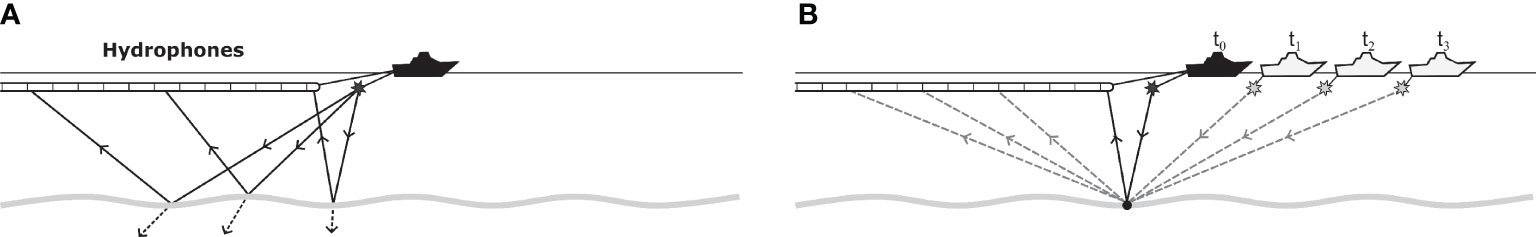
Figure 1 Principles of seismic oceanography. (A) Cartoon showing single release of energy by acoustic source. Black star = acoustic source; undulating gray line = change in oceanic temperature and/or salinity; solid black lines with arrows = travel paths for three example sets of incident and reflected sound waves; dashed black lines with arrows = transmitted sound waves. In reality, sound waves travel out from acoustic source in all directions and are recorded at every hydrophone along cable. (B) Cartoon illustrating repeated sampling of same spatial point by multiple firings of acoustic source. Black dot = repeatedly sampled point; black star = acoustic source at time t₀; solid black lines with arrows = travel path for sound waves excited at time t₀ and reflected from black dot; gray stars = acoustic source at later times t₁, t₂, t₃; dashed gray lines with arrows = travel paths for sound waves excited at times t₁, t₂, t₃ and reflected from black dot. Note that cable of hydrophones is not illustrated for times t₁, t₂, t₃. For more complete introductions to acquisition of seismic oceanographic data, see Fer and Holbrook (2009), Ruddick et al. (2009) and Holbrook (2009).

Use of underwater sound for remote sensing of internal oceanic structure is, of course, not new. For decades, ocean-bottom echosounders have monitored thermocline depths, acoustic tomographic systems have detected basin-wide temperature changes, and acoustic Doppler current profilers (ADCPs) have measured current velocities (Rossby, 1969; Munk and Wunsch, 1979; Pinkel, 1979). High-frequency (i.e., ≳ 10 kHz) acoustic surveys provide spectacular images of near-surface internal waves and capture the intensity of turbulent mixing (Figures 2B, C; e.g., Proni and Apel, 1975; Geyer et al., 2010; Lavery et al., 2013). Seismic oceanography is distinguished, however, from other acoustic imaging methods in two ways (Fer and Holbrook, 2009). First, it uses low-frequency (i.e., ≲ 100 Hz) sound that does not attenuate rapidly with depth². Second, each imaged point is repeatedly sampled over a time interval of ≲ 30 minutes by different configurations of acoustic source and hydrophones, increasing the signal-to-noise ratio (Figure 1B). These distinctive features lend seismic oceanography a unique combination of three key characteristics:

● Multi-dimensional observation of the ocean at high spatial resolution. Seismic oceanography provides a two-dimensional, and often three-dimensional, view of the ocean at horizontal and vertical resolutions on the order of 10 m. Other observational tools may achieve higher spatial resolutions, but usually provide measurements in only one dimension.

● Penetration to abyssal depths. Unlike higher-frequency acoustic methods, seismic oceanography captures thermohaline structure down to depths of several kilometers. This capability allows observation of abyssal regions that are otherwise undersampled.

● Horizontal coverage over hundreds of kilometers. Seismic data are continuously recorded along ≲ 1,000-km-long transects. This coverage provides a holistic view of structures such as eddies that are otherwise only intermittently sampled (e.g., by dropped probes).

FIGURE 2

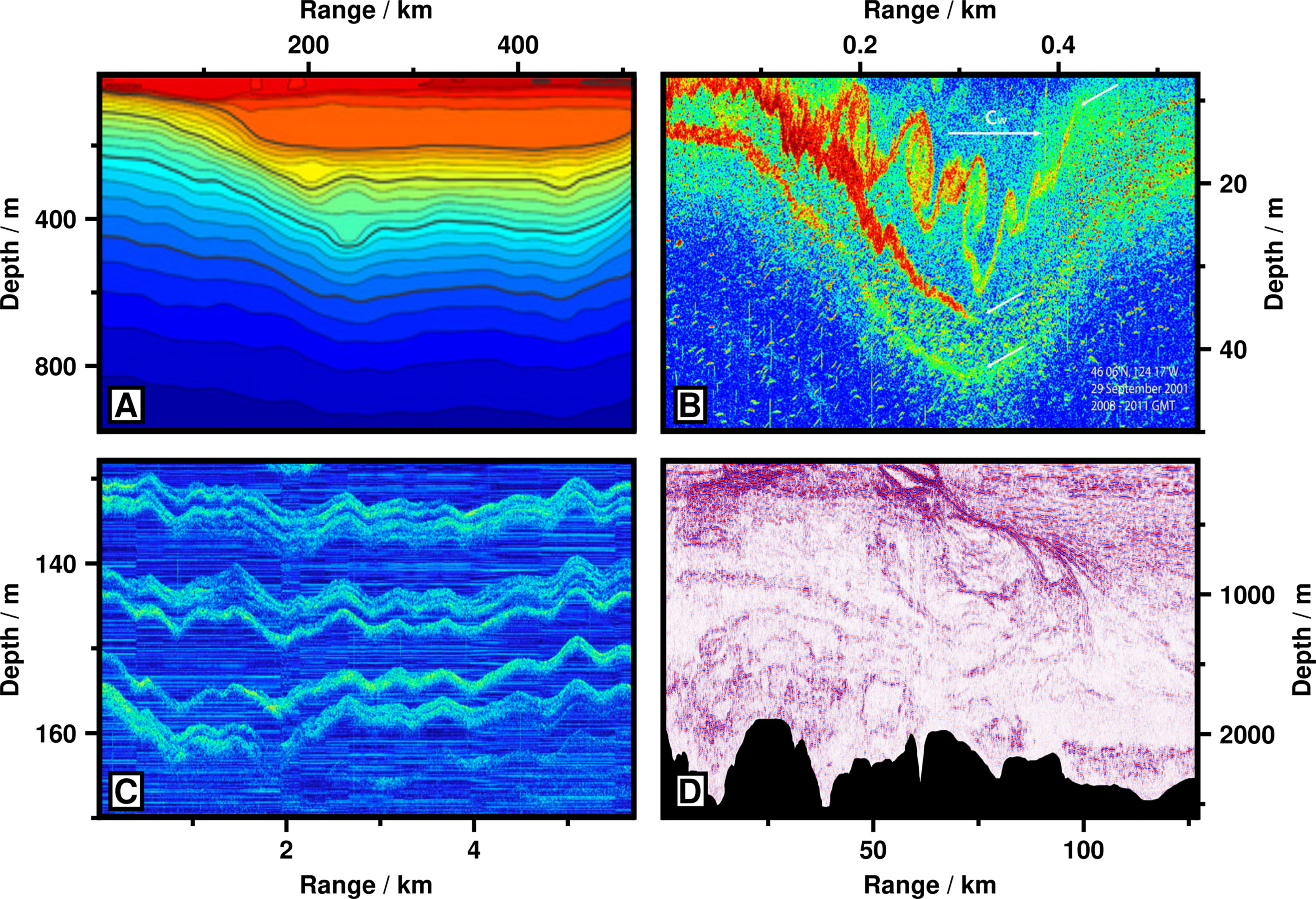
Figure 2 Comparison of seismic oceanography to other observational techniques. (A) Temperature section interpolated from measurements made by glider in Gulf of Mexico (after Figure 3D of Meunier et al., 2019). Red = warmer water; blue = cooler water; vertical resolution ≈ 2 m; horizontal resolution ≈ 2,000 m. (B) High-frequency (∼ 120 kHz) echosounder image of Kelvin-Helmholtz instabilities within internal solitary wave above Oregon continental shelf (after Figure 14 of Moum et al., 2003). Red = high acoustic intensity; blue = low acoustic intensity; vertical resolution ≈ 0.04 m; horizontal resolution ≈ 3 m at depth of 30 m. (C) High-frequency (∼ 15–25 kHz) echosounder image of thermohaline staircase in Arctic Ocean (after Figure 5 of Stranne et al., 2017). Brighter colors indicate higher acoustic amplitudes; vertical resolution ≈ 0.1 m; horizontal resolution ≈ 15 m at depth of 150 m. (D) Seismic oceanographic image of oceanic front at Brazil-Malvinas Confluence (after Figure 3A of Gunn et al., 2020b). Red colors = positive acoustic amplitudes; blue colors = negative acoustic amplitudes; black region = seafloor; vertical and horizontal resolutions ∼ O (10) m. Note different ranges and depths of four panels.

Due to these characteristics, seismic oceanography has provided uniquely detailed images of features such as fronts, tidal beams, eddies, thermohaline staircases and turbid layers (e.g., Nakamura et al., 2006; Holbrook et al., 2009; Pinheiro et al., 2010; Fer et al., 2010; Vsemirnova et al., 2012; Figure 2D). Importantly, seismic records provide not only spectacular images, but have yielded quantitative insight into dynamical phenomena including thermohaline interleaving, propagation of internal waves, and turbulent mixing (e.g., Papenberg et al., 2010; Tang et al., 2014; Falder et al., 2016; Figure 3). Reviews of topics as wide-ranging as stratified turbulence, circumpolar currents and submesoscale flow have cited results from seismic oceanography (e.g., Riley and Lindborg, 2008; Thompson et al., 2018; McWilliams, 2019). In total, more than one hundred peer-reviewed research papers have now presented seismic oceanographic data (Appendix A; Table A; see Supplementary Material for all appendices and tables).

FIGURE 3

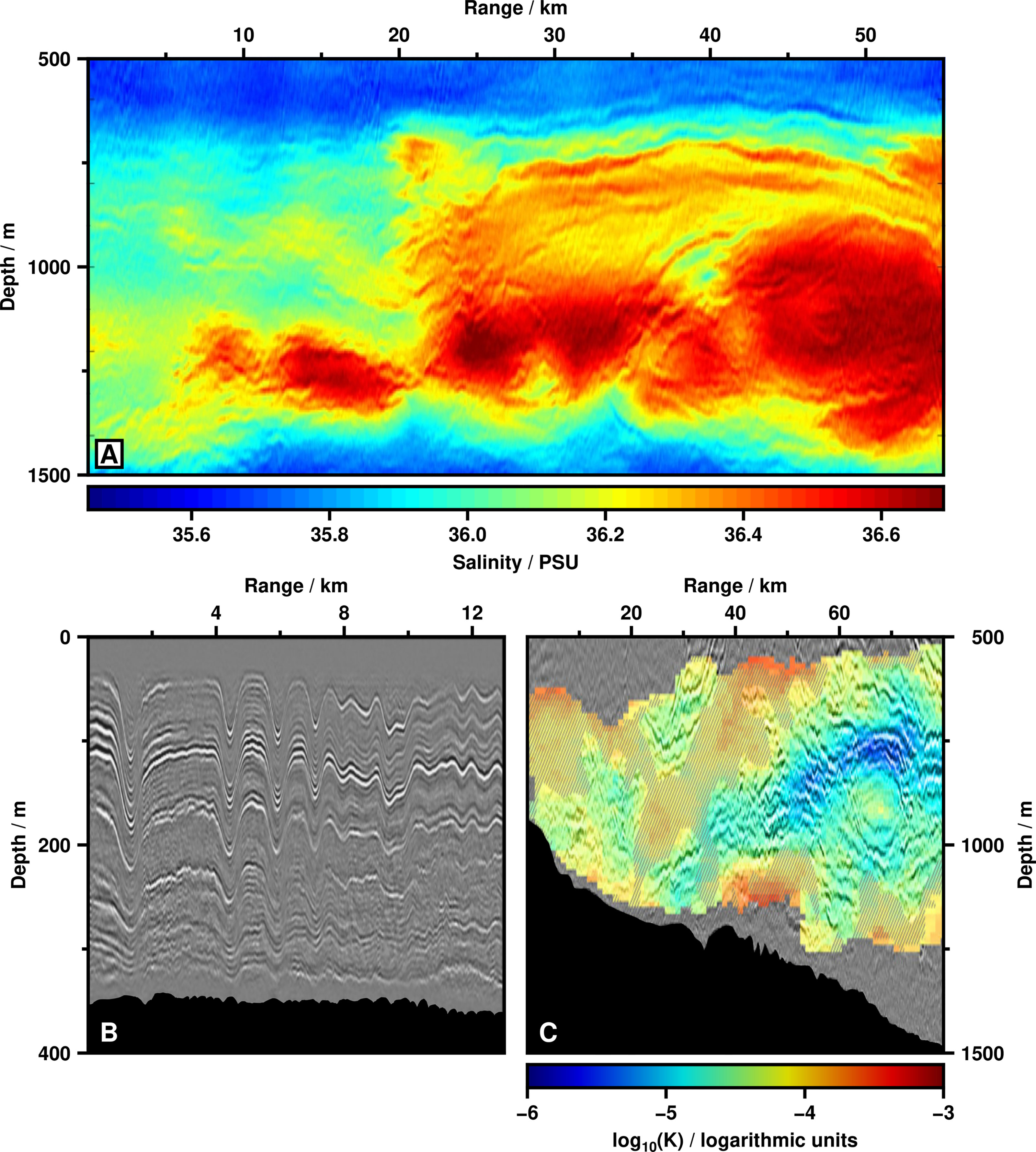
Figure 3 Initial successes of seismic oceanography. (A) Values of salinity inverted from seismic oceanographic image of eddy of Mediterranean Water in Gulf of Cadiz (after Figure 6 of Dagnino et al., 2016). Note finely resolved layering along upper side of eddy. (B) Internal solitary waves captured in seismic oceanographic image from South China Sea (after Figure 2 of Tang et al., 2016). Grayscale represents response of thermohaline structure to seismic waves; black region = seafloor. Internal-wave velocities can be estimated from seismic records. (C) Spatial map of diapycnal diffusivity, K, estimated from seismic oceanographic image above Falkland Plateau (after Figure 15b of Falder et al., 2016). Grayscale = seismic image; colored overlay = estimates of K; hashed pattern = areas where estimates are less certain; black region = seafloor. Note depressed values of K above eddy imaged at range of ∼ 60–70 km.

Despite these successes, seismic oceanography has struggled to establish itself as a standard observational tool. This slow development has two causes. First, the field has been hindered by practical challenges associated with acquiring data and with analyzing records in a consistent and reliable way. Second, and more fundamentally, many physical oceanographers regard the field as a curiosity, with no clear vision or scientific application. To progress further, the seismic oceanographic community needs to identify key scientific questions that it can systematically address.

Here, we discuss the practical challenges that face seismic oceanography and suggest ways in which they can be overcome (Section 2). We then discuss how seismic oceanography can address scientific questions that other tools cannot answer (Section 3). Finally, we outline ways in which the seismic oceanographic community can implement these solutions by agreeing on priorities and by working together on collaborative projects (Section 4).

2 How can Seismic Oceanography Overcome its Practical Challenges?

Seismic oceanography is faced by three practical challenges. Previous works have outlined possible solutions to one or more of these challenges (e.g., Jones et al., 2008; Holbrook, 2009; Jones et al., 2010; Buffett and Carbonell, 2011; Ruddick, 2018). Here, we build on these works to develop a comprehensive strategy for overcoming all three challenges.

2.1 How Can We Acquire Seismic Oceanographic Data?

Perhaps the greatest practical obstacle to further development of seismic oceanography is the logistical difficulty and high cost of acquiring data. Conventional seismic reflection surveys require specialized vessels that are capable of towing powerful acoustic sources and long cables of hydrophones. A small number of research bodies maintain such vessels (e.g., the Alfred Wegener Institute, Germany; the Natural Environmental Research Council, UK; the University-National Oceanographic Laboratory System, USA). Access to ship time is limited and surveys are up to five times more expensive than other ocean-going research cruises (National Research Council, 2015; National Science Foundation, 2016). Chartering of independent seismic exploration companies can cost up to three times as much again (National Science Foundation, 2016). There are two possible solutions to the challenge of high cost and logistical difficulty.

2.1.1 Development of New Seismic Systems

First, data could be acquired using systems that are specially designed for seismic oceanography (e.g., Ruddick, 2018). These systems could be optimized to reduce costs and to target specific oceanographic phenomena. Ideally, they would be deployed alongside other observational instruments and would not require use of specialized vessels. The most obvious way to lower costs and improve deployability is to use weaker acoustic sources and shorter cables of hydrophones. Weaker acoustic sources produce higher-frequency (i.e., ≳ 100 Hz) sound waves that provide increased spatial resolution, but the signal-to-noise ratio degrades more quickly with depth (Geli et al., 2009; Hobbs et al., 2009). Although this degradation can be partially compensated for by more frequent firing of the source and by a denser spacing of hydrophones, it seems unlikely that higher-frequency sources will be capable of clearly imaging the water column to abyssal depths (Nakamura et al., 2006). Instead, higher-frequency seismic systems could be optimized for imaging of relatively shallow structures such as seasonal thermoclines (Piété et al., 2013; Ker et al., 2015; Sallares et al., 2016; Mojica et al., 2018). When combined with direct measurements of properties such as temperature and salinity, they could form an excellent tool for investigation of processes that are too coarse to be detected by high-frequency echosounders and yet too fine to be detected by conventional seismic systems.

2.1.2 Use of Existing Datasets

An alternative solution to the difficulty of acquiring new seismic reflection data is to analyze existing records. An overwhelming majority of these records have been acquired by seismic exploration companies, which spend billions of dollars each year on new datasets (McBarnet, 2013). As a consequence, these companies can afford equipment and modes of operation that are far beyond the budgets of research organisations. Commercial seismic records are thus likely to have higher signal-to-noise ratios and to be more accurately spatially positioned than records acquired for scientific research. Dense layouts of overlapping transects are often acquired in a small area over a period of several weeks or months, allowing the temporal evolution of oceanographic phenomena to be tracked (e.g., Dickinson et al., 2020; Gunn et al., 2020b; Zou et al., 2020; Gunn et al., 2021). Many commercial exploration vessels carry several parallel cables of hydrophones, enabling imaging of thermohaline structure in three spatial dimensions (these surveys are known as three-dimensional; Blacic and Holbrook, 2010; Bakhtiari Rad and Macelloni, 2020; Zou et al., 2021).

Existing surveys are concentrated above continental shelves and slopes, which exploration companies have targeted since they house economically valuable reserves of oil and gas (Figure 4A). Recent observational, theoretical and computational work suggests that the mixing that drives oceanic circulation is most intense above these continental margins and above other topographically rough features such as mid-ocean ridges and seamount flanks (e.g., Waterhouse et al., 2014; Ferrari et al., 2016; McDougall and Ferrari, 2017; Drake et al., 2020). Continental margins also host western boundary currents that transport significant quantities of heat, salt and nutrients (e.g., Stommel, 1948; Hu et al., 2015; Buckley and Marshall, 2016). In a warming climate, the intensity and position of these currents is likely to change markedly, yet there are limited direct observations of their magnitude and variability (e.g., Wu et al., 2012; Yang et al., 2016). Existing seismic records span several decades and provide a dataset of unprecedented size and coverage that can be used to investigate in detail these critically important interactions above continental margins.

FIGURE 4

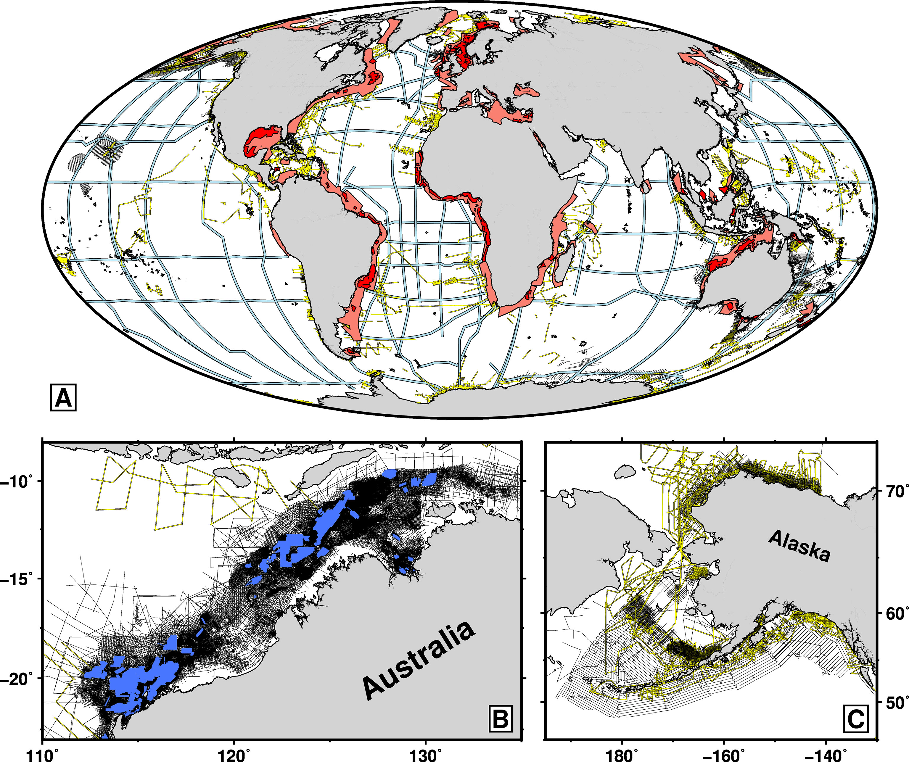
Figure 4 Existing marine seismic reflection data. (A) Global distribution. Light red polygons = regions covered by two-dimensional (i.e., single-cable) surveys acquired by seismic exploration companies; dark red polygons = regions covered by three-dimensional (i.e., multi-cable) surveys acquired by seismic exploration companies; thin black lines = publicly available two-dimensional surveys acquired by seismic exploration companies in other regions; yellow lines = publicly available two-dimensional surveys acquired by research institutions; light blue lines = hydrographic transects of World Ocean Circulation Experiment (WOCE; www.ewoce.org). Red polygons were traced from the websites of the five largest exploration companies (CGG, ION, PGS, Schlumberger, TGS) and represent > 6.3 million km of two-dimensional seismic data and > 5.5 million km² of three-dimensional seismic data. Publicly available data were downloaded from a range of online repositories (note that plotted transects represent only a small subset of all existing data). (B) Zoom of Australia’s Northwest Shelf showing only publicly available seismic data. Blue polygons = three-dimensional commercial surveys made available through the National Offshore Petroleum Information Management System (NOPIMS; www.ga.gov.au/nopims). (C) Zoom of the Gulf of Alaska and the Bering, Chukchi and Beaufort Seas showing only publicly available seismic data. Note that WOCE transects are not plotted in panels (B) or (C). See Supplementary Material for further details of data provenance.

Thanks to burgeoning open-access initiatives, an increasing number of both academic and commercial datasets are being made publicly available (Figures 4B, C; Appendix B). Researchers need only cover data-dearchiving and data-shipment costs. Access to other, privately held, commercial datasets might be most easily gained through formation of an international collaboration for all seismic oceanography researchers (Jones et al., 2010; Buffett and Carbonell, 2011). Many seismic exploration companies are currently seeking ways to improve their public image by promoting independent scientific research. Supporting seismic oceanography is particularly attractive since only commercially worthless water-column reflections, and not commercially valuable subsurface reflections, need be supplied.

2.2 How Can We Benchmark Seismic Oceanographic Data?

Estimation of accurate quantitative results from seismic oceanographic datasets requires a reliable understanding of the correspondence between seismic records and hydrographic properties. However, it has remained difficult to gain such an understanding since the strength and form of recorded seismic amplitudes are functions of many variables, which depend both on local thermohaline structure and on the seismic acquisition system. Key questions fall into three areas:

● Hydrographic sensitivity: What are the smallest changes in temperature and salinity which seismic reflection surveys can detect? How well do these changes correspond to changes in density? On what spatial length scales can these changes be detected?

● Temporal blurring: How does motion of thermohaline structure, acoustic source and recording system affect observation of features that are repeatedly sampled during periods of ≲ 30 minutes?

● Seismic system: How do the answers to these questions change with variations in acoustic frequency and in design of the recording system?

Studies have addressed one or more of these questions in isolated circumstances (Appendix C; Table C). To analyze seismic data more widely, it would be helpful to systematically investigate these questions across the full range of oceanographic settings. This investigation can be carried out in two ways.

2.2.1 Field Datasets With Hydrographic Calibration

First, seismic records can be compared to coincident, direct measurements of properties such as temperature, salinity and current velocity. These comparisons aid interpretation of imaged phenomena and guide estimation of quantities such as temperature, salinity and diapycnal diffusivity from seismic images (e.g., Papenberg et al., 2010; Holbrook et al., 2013). Coupling seismic records to more familiar oceanographic measurements is also likely to encourage widespread acceptance of seismic oceanography (Ruddick, 2018). Twenty-four existing datasets have such ancillary data and have been used for seismic oceanographic research (Appendix C.1; Table C.1). Datasets with hydrographic calibration could in future be acquired by combining specially designed seismic systems of the kind discussed in Section 2.1.1 with instruments such as expendable bathythermographs (XBTs), ADCPs, and microstructure profilers. However, seismic exploration companies, which carry out the majority of surveys, do not routinely acquire high-quality hydrographic data. More fundamentally, the unique coverage and spatial resolution of seismic reflection data means that coincident hydrographic measurements cannot capture all relevant scales.

2.2.2 Numerical Modeling

Numerical modeling and synthetic datasets offer a way to comprehensively explore scales that hydrographic calibration cannot access. An ideal numerical model would include realistic descriptions of two elements. First, thermohaline structure would be described by a time-variant fluid-dynamical model that resolves time scales of minutes to days and vertical and horizontal length scales of ∼0(1) m (Ménesguen et al., 2018). Second, this simulated structure would be acoustically probed by a modeled seismic acquisition system travelling at finite speed. Models with these two elements could faithfully replicate the characteristics of seismic surveys in a range of oceanographic conditions.

Existing studies have built numerical models of varying sophistication (Appendix C.2; Tables C.2.1, C.2.2). These models have been used to investigate the effect of fluid flow on wave propagation and on blurring of seismic reflections, to assess correspondence between reflections and isopycnals, to quantify errors in imaging of deep structure due to non-homogeneous near-surface waters, and to simulate the characteristics of new seismic oceanographic acquisition systems (e.g., Vsemirnova et al., 2009; Ji and Lin, 2013; Holbrook et al., 2013; Ji et al., 2013; Biescas et al., 2016). Previous work must now be built upon to form a standardized toolkit for modeling of seismic reflection profiling of thermohaline structure. Using this toolkit, the accuracy of quantitative results derived from seismic images can be assessed.

2.3 How Can We Analyze Seismic Oceanographic Data?

Development of seismic oceanography has to date been advanced by disparate groups of researchers, each of which has developed its own computer codes for signal processing and interpretation. Many of these codes either rely on proprietary software or have not been made publicly available (see Table D). Lack of open-source code hampers replication of results and discourages scientists who do not have a background in seismic signal processing.

To realize the full potential of seismic oceanography, the community must now develop standardized open-source codes which can be used with a broad range of seismic datasets. Key to standardization will be rigorous investigation of the effects of different workflows on the accuracy of results (see Appendix D for a discussion of workflows for constructing seismic images). Here, we focus on three fields that comprise the majority of existing quantitative work and which are ripe for standardization:

● Hydrographic Inversion. Estimation of sound speed, temperature, salinity and density.

● Propagation of Internal Waves. Characterization of the size, velocity and decay of internal waves.

● Spectral Analysis. Analysis of internal waves and turbulence using wavenumber spectra.

For each of these fields, we summarize previous work, suggest potential future applications, and highlight selected outstanding questions.

2.3.1 Hydrographic Inversion

Propagation of low-frequency acoustic waves within the oceanic water column is governed by changes in sound speed and, to a much smaller extent, in density (Ruddick et al., 2009; Sallares et al., 2009). Sound speed can thus be directly estimated from seismic data and mapped into values of temperature and salinity using an assumed temperature-salinity relationship and the hydrographic equation of state (see Appendix D.1and Table D.1 for a summary of proposed methods). Hydrographic inversion has been used, for example, to investigate stirring at baroclinic fronts, to describe temperature variance in turbulent waters above a continental slope, and to reassess heat transport onto the Antarctic shelf (Biescas et al., 2014; Minakov et al., 2017; Gunn et al., 2018). Inversion results can also act as constraints for other calculations that are made using seismic records (e.g., estimation of diapycnal heat flux, Gunn et al., 2021; see Sections 3.1 and 3.2). Key questions for further development of hydrographic inversion include:

● How accurate can inversion results be in the absence of nearby hydrographic data? See Bornstein et al. (2013), Padhi et al. (2015) and Blacic et al. (2016).

● What are the smallest and greatest spatial scales that can be recovered? See Blacic et al. (2016), Minakov et al. (2017) and Gunn et al. (2018).

● Can useful inversion results be obtained from records in which water-column reflections are very faint or absent?

2.3.2 Propagation of Internal Waves

Seismic oceanographic images often display prominent internal waves, including tidal beams, lee waves and trains of solitary waves (e.g., Holbrook et al., 2009; Eakin et al., 2011; Tang et al., 2015). The velocities of these waves can be estimated by analyzing changes in reflection amplitude during the interval of ≲ 30 minutes within which a single point is sampled (Appendix D.2; Table D.2). This approach has shed light on stirring at oceanic fronts, on the evolution of solitary waves, and on heat transport by intrathermocline eddies (Sheen et al., 2012; Tang et al., 2014; Gunn et al., 2018). Blacic and Holbrook (2010) and Zou et al. (2020) suggest how these analyses could be extended to mapping internal waves in three dimensions. This mapping could greatly improve our understanding of internal-wave-driven mixing of energy and material, which plays a critical role in global climate (e.g., Helfrich and Melville, 2006; Legg, 2021). Outstanding questions for seismic oceanographic estimation of internal-wave velocities include:

● To what extent is it possible to decouple the velocities of internal waves from the velocities of background currents?

● How does the accuracy of estimated velocities vary with duration of observation?

● How sensitive are estimated internal-wave velocities to errors in the profiles of sound speed that are used to spatially reposition reflections? See Klaeschen et al. (2009).

2.3.3 Spectral Analysis

In addition to imaging clearly visible internal waves, seismic oceanographic data capture the signals of the background internal wave field and of turbulent motions. These signals have most commonly been analyzed by computing horizontal-wavenumber spectra from the vertical displacements of tracked seismic reflections (e.g., Holbrook and Fer, 2005; Appendix D.3; Table D.3). This approach has been exploited to investigate the nature of the dynamical transition from internal waves to turbulence, to link intensity of turbulent overturning to submesoscale structure, and to estimate diapycnal mixing above regions of rough bathymetry (e.g., Falder et al., 2016; Tang et al., 2020; Tang et al., 2021). Fortin et al. (2016) suggest how spectra can be estimated from regions of a seismic image in which reflections cannot be tracked. To develop a consistent and reliable method for spectrally analyzing seismic oceanographic images, the following outstanding questions must be addressed:

● How closely must reflections track isopycnals for results to be useful? What information can be extracted from the spectra of reflections that do not track isopycnals? See Meunier et al. (2019).

● How severely are spectra distorted by temporal blurring? See Vsemirnova et al. (2009) and Falder et al. (2016).

● How are spectra affected by use of different methods for mapping of recorded seismic amplitudes into spatial images? Which method is most appropriate? See Fortin and Holbrook (2009) and Holbrook et al. (2013).

In future, spectra could potentially be computed directly from seismically estimated sections of temperature and salinity, avoiding the need to track reflections (see Section 3.2; Xiao et al., 2021).

3 What Problems can Seismic Oceanography Solve?

To gain widespread acceptance, the seismic oceanographic community must identify ways in which the datasets and tools discussed in Section 2 can be used to rapidly improve our understanding of oceanic circulation. This circulation encompasses myriad processes that continuously interact on a wide range of time and length scales. No single theory or set of observations can hope to simultaneously capture all of these interactions. Instead, oceanographers conceptualize circulation as a collection of discrete phenomena (e.g., Ferrari and Wunsch, 2009). Transfer of energy between these phenomena is described by parametrizations that are based on a combination of theoretical and empirical evidence (e.g., Garrett, 2006; Polzin et al., 2014; McWilliams, 2017; de Lavergne et al., 2020).

Seismic oceanography straddles a unique combination of scales and is thus ideally placed to revolutionize our understanding of several processes and parametrizations (see Figure 5). Here, we outline three areas in which the seismic method can provide key insights within the next decade.

FIGURE 5

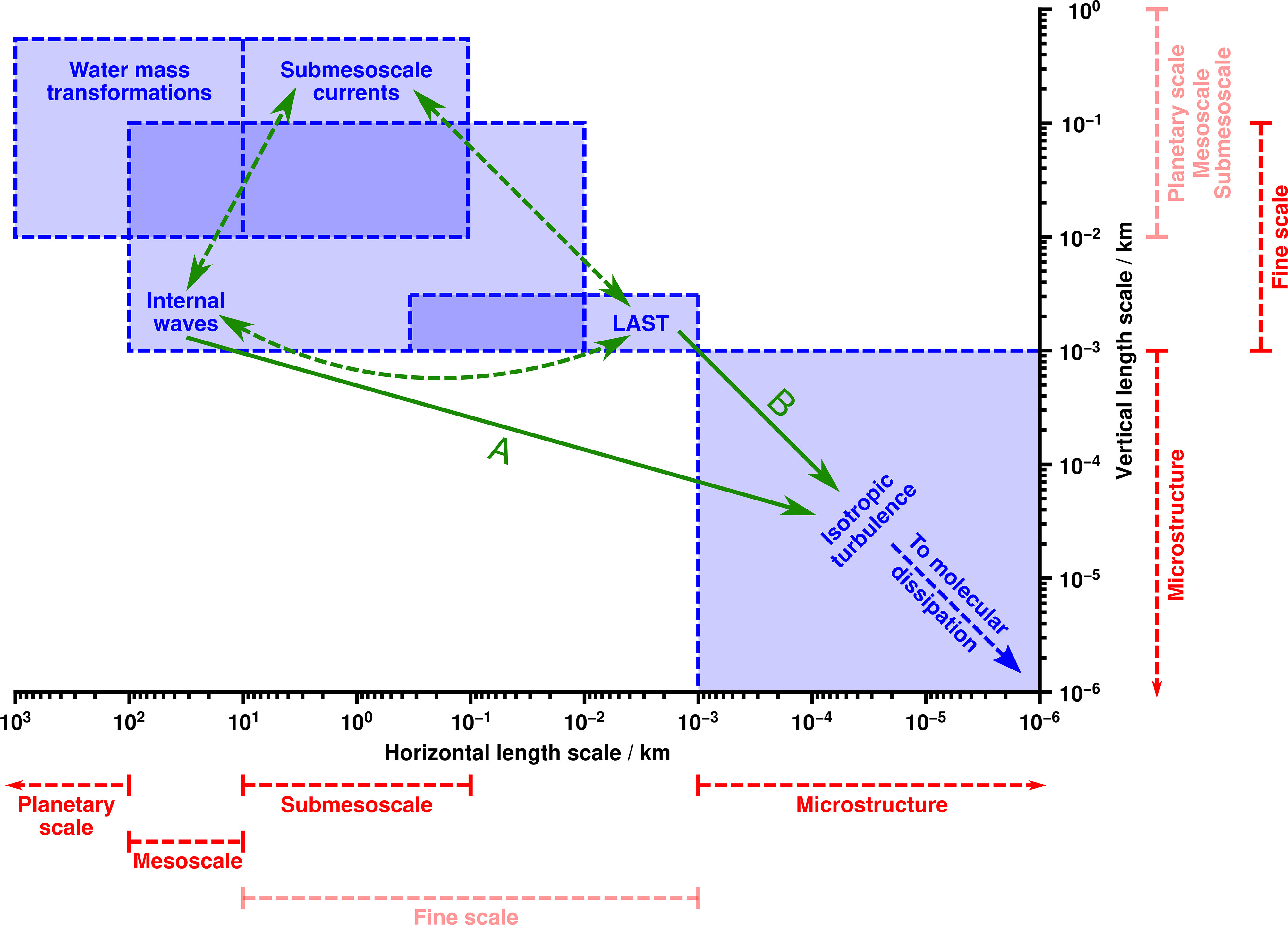
Figure 5 Cartoon showing approximate length scales of processes that can be investigated using seismic oceanography. Red dashed bars show approximate ranges³ of commonly used descriptive terms. (The term fine scale was coined to describe vertically varying structure, and its horizontal extent is not clearly defined. Planetary scale, mesoscale and submesoscale are predominantly used to describe horizontal length scales.) Blue boxes show approximate extents of selected phenomena. LAST = layered anisotropic stratified turbulence⁵. Green arrows show possible parametrizations describing transfer of energy. Solid arrow labeled A = fine-scale parametrizations; solid arrow labeled B = assumption of continuity between LAST and inertial-convective regime of isotropic turbulence⁵ ; dashed green arrows = other parametrizations that seismic oceanography could inform. Note that boundaries between phenomena are much more gradational than depicted. Only phenomena referred to in this article are shown. Inspired by Figure 1 of McWilliams (2016) and Figure 1 of Ruddick (2018).

3.1 Turbulent Mixing

It is widely accepted that mechanical mixing⁴ by turbulent motions is key to maintaining global overturning circulation (e.g., Munk, 1966; Wunsch and Ferrari, 2004). Observations since the 1990s have shown that turbulent mixing is concentrated above regions of rough bathymetry and at the edges of ocean basins (e.g., Polzin et al., 1997; Mauritzen et al., 2002; Naveira Garabato et al., 2019). These observations have spurred theoretical advances which suggest that mixing in narrow boundary layers forms a critical part of oceanic circulation (Levy et al., 2012; Ferrari et al., 2016; McDougall and Ferrari, 2017; Drake et al., 2020). Further measurements are now needed to refine these theories and to tune climate models (e.g., Mashayek et al., 2015; Mashayek et al., 2017; MacKinnon et al., 2017).

Unfortunately, oceanic turbulence is difficult to sample since it is highly intermittent in both space and time (Ivey et al., 2008; Shroyer et al., 2018; Cael and Mashayek, 2021). Fast-response thermistors and shear probes, which have most commonly been deployed as vertically dropped microstructure profilers, resolve isotropic turbulent⁵ fluctuations on length scales as small as ∼0(1) mm (Figure 5; e.g., Schmitt et al., 1988; Lueck et al., 2002; Lozovatsky et al., 2019). However, microstructure profiles are uncommon and sparsely distributed. For instance, in compiling a global database of turbulence measurements, Waterhouse et al. (2014) found only ∼5,200 profiles of vertical shear. Such small numbers of measurements cannot constrain the global distribution of turbulence.

To overcome this problem, many studies have sought to infer the strength of turbulence using observations of internal waves on vertical length scales of ∼0(1-10) m (Figure 5; Gregg, 1989; Wijesekera et al., 1993; MacKinnon and Gregg, 2003; Polzin et al., 2014; Ijichi and Hibiya, 2015). These inferences, which are known as fine-scale parametrizations, have underpinned attempts to map the global distribution of mixing using measurements made by conductivity-temperature-depth (CTD) profilers and Argo floats (Whalen et al., 2012; Waterhouse et al., 2014; Whalen et al., 2015; Kunze, 2017). However, few studies have benchmarked the results of fine-scale parametrizations against direct measurements of turbulence (e.g., Liang et al., 2018; Takahashi and Hibiya, 2019; Takahashi and Hibiya, 2021; Fine et al., 2021).

Instruments that record structure on horizontal scales of ≳ O(10) m offer an alternative way to both directly measure turbulence and benchmark fine-scale parametrizations (Moum, 2021). On horizontal length scales of ≲ 300 m, observations reveal a regime of layered anisotropic stratified turbulence (LAST)⁵ that can be straightforwardly related to the intensity of isotropic turbulence (Figure 5; Brethouwer et al., 2007; Klymak and Moum, 2007b; Maffioli and Davidson, 2016; Kunze, 2019). Internal-wave signals on greater horizontal length scales can be analyzed using modified fine-scale parametrizations to yield indirect estimates of the strength of turbulent mixing (e.g., Klymak and Moum, 2007a; Sheen et al., 2009; Dickinson et al., 2017).

The horizontal signals of internal waves and LAST are captured both by towed instruments and by seismic oceanography (e.g., LaFond, 1963; McKean and Ewart, 1974; Holbrook and Fer, 2005; Holbrook et al., 2013). However, seismic oceanography is distinguished by its ability to record unprecedentedly large volumes of data in short periods of time. For instance, one 175-km-long seismic image acquired over a 20-hour period shows reflective boundaries with a cumulative length of more than 5,000 km (Dickinson et al., 2017). This length is over thirty times greater than the combined length of the datasets on which Garrett and Munk (1972) based the horizontal-wavenumber description of their original semi-empirical internal-wave spectrum. Rapid acquisition also distinguishes seismic oceanography from more recent campaigns that have acquired horizontal measurements over periods of several weeks (e.g., Ferrari and Rudnick, 2000).

Spectral analysis of extensive seismic oceanographic datasets thus has the potential to provide a global catalogue of oceanic horizontal-wavenumber spectra that is unrivalled in size (cf. Polzin and Lvov, 2011). Statistical investigation of this catalogue could address questions that include:

● How accurate is the Garrett-Munk spectrum for internal waves? How do the spectral properties of internal waves vary in different oceanic environments? See Levine (2002), Polzin and Lvov (2011)and Pinkel (2020).

● What is the nature of the dynamical transition between internal waves and LAST on horizontal length scales of ∼0(100) m? See Falder et al. (2016), Sallares et al. (2016), Kunze (2019) and Howland et al. (2020).

● How accurate are existing fine-scale parametrizations when applied to horizontal-wavenumber spectra⁶? Do different parametrizations work better in different oceanic environments? Is it possible to formulate new parametrizations that better apply to horizontal-wavenumber spectra? See MacKinnon and Gregg (2003), Klymak and Moum (2007a), Hibiya et al. (2012), Polzin et al. (2014), Waterman et al. (2014) and Ijichi and Hibiya (2015).

Perhaps most importantly, seismic oceanography offers a way to map the intensity of turbulent mixing in unprecedented two-dimensional detail across sections that are hundreds of kilometers in length (e.g., Tang et al., 2021; Wei et al., 2022). Advances in oceanographic instrumentation are providing new tools that can be integrated into future seismic surveys to benchmark estimates of mixing (Frajka-Williams et al., 2022). Shear probes will be mounted on Argo floats, whilst expendable profilers will measure velocity fluctuations to depths of ~ 6,000 m (e.g., Shroyer et al., 2016; Shang et al., 2017; Roemmich et al., 2019). Seismometers will record turbulent flow in narrow boundary layers above the ocean floor (Yang et al., 2021). Once seismic methods for estimating mixing have been accurately calibrated using these tools and using numerical simulations, existing seismic datasets will provide a way to investigate possible changes in oceanic mixing during the previous four decades, when few other measurements were available.

3.2 Submesoscale Currents

The submesoscale range plays host not only to internal waves, but to a menagerie of other phenomena that evolve on time scales of hours to days (Figure 5; Thomas et al., 2008; Callies et al., 2020). These non-internal-wave phenomena, which we collectively refer to as submesoscale currents⁷ following McWilliams (2019), are thought to be vital in sustaining ecosystems and in modulating exchange of energy between mesoscale motions and microscale turbulent flows (e.g., Levy et al., 2018; Naveira Garabato et al., 2022). Unfortunately, they are difficult to discern in observational time series and in measurements made by vertically dropped instruments (McWilliams, 2016). As a result, most in situ observations have been obtained using platforms that sample the ocean horizontally, such as towed thermistors or ADCPs (e.g., Samelson and Paulson, 1988; Klymak and Moum, 2007a; Rocha et al., 2016; Qiu et al., 2017).

A more complete description of submesoscale currents requires rapid two- or three-dimensional sampling (McWilliams, 2019). Although gliders provide quasi-two-dimensional observations, they travel at slow horizontal speeds of ∼0.3 m s^-1and probably only resolve features at horizontal scales greater than ∼30 km (e.g., Figure 2A; Rudnick and Cole, 2011; Rudnick, 2016). A few field campaigns have sought three-dimensional descriptions by tracking the spread of inert tracers, by carrying out surveys with two closely spaced ships, and by combining moored, towed and dropped instruments with airborne sensors and with autonomous floats, drifters and gliders (e.g., Allen and Naveira Garabato, 2012; Shcherbina et al., 2013; Shcherbina et al., 2015; Pascual et al., 2017; Marmorino et al., 2018). However, these campaigns have small geographical extents and are limited to the upper ~ 500 m of the ocean. Satellites and airborne instrumentation have revolutionized our understanding of submesoscale activity at the sea surface (e.g., Gower et al., 1980; Munk et al., 2000; Jolliff et al., 2019; Klein et al., 2019; Martínez-Moreno et al., 2021). However, it is not well known how closely these surface motions correspond to flow at depth (e.g., Wang et al., 2010; Callies and Ferrari, 2013).

In addition to being difficult to observe, submesoscale currents are difficult to theoretically describe (e.g., McWilliams, 2010; McWilliams, 2017). As a result, developments in our understanding have been largely driven by numerical simulations (McWilliams, 2019). At present, most simulations are validated by comparison to satellite or radar observations of sea-surface height and temperature (e.g., Delandmeter et al., 2017; Schubert et al., 2019; Bashmachnikov et al., 2020; Chrysagi et al., 2021). Few studies have compared simulations to subsurface observations (e.g., Rocha et al., 2016; Liu et al., 2017; Viglione et al., 2018). Improving our ability to observe submesoscale currents and to benchmark simulations now requires an efficient way to rapidly sample thermohaline structure between the sea surface and the seafloor.

Seismic oceanography offers an unrivalled means of achieving this sampling. Unlike gliders, seismic vessels move at fast speeds of ∼ 2.5–3  m s^-1, allowing surveys to capture submesoscale structures that evolve on time scales of hours to days. This ability can be exploited in three ways. First, seismic images can reveal the geometries and distributions of subsurface submesoscale structures in unprecedented detail. For instance, Song et al. (2011) present a seismic image which shows how submesoscale coherent vortices generate thermohaline intrusions with forms that are unanticipated by theory. By combining seismic images with inverted sections of temperature, salinity and density, Gunn et al. (2020b) show how submesoscale lenses and filaments interact with a deep-seated oceanic front. Seismic oceanography’s ability to visualise submesoscale features can address questions such as:

● How abundant are submesoscale coherent vortices? How quickly do they evolve? See Gunn et al. (2018), Gula et al. (2019), Steinberg et al. (2019), Archer et al. (2020), McCoy et al. (2020) and Tang et al. (2020).

● How widespread are submesoscale fronts? To what depth do these fronts extend? How are they influenced by the presence of permanent fronts between water masses? See Ramachandran et al. (2014), Pascual et al. (2017), Siegelman et al. (2019), Gunn et al. (2020b) and Giddy et al. (2021).

● How does the size and form of imaged submesoscale structures vary with depth and with proximity to rough topography? See de Lavergne et al. (2016), Dauhajre et al. (2017), Ruan et al. (2017), Callies (2018) and Wenegrat et al. (2018).

Second, seismic oceanography can probe the statistical signatures of submesoscale currents. To date, few observational studies have resolved along-isobar and along-isopycnal hydrographic variations on submesoscale length scales, and the distribution of potential energy in the submesoscale range is poorly known (e.g., Cole and Rudnick, 2012; Callies and Ferrari, 2013; Schönau and Rudnick, 2015; Itoh and Rudnick, 2017). Improved observations will show which processes dominate transfer of energy and how they contribute to lateral stirring of water masses (e.g., Rudnick and Martin, 2002; Johnson et al., 2012; Jaeger and Mahadevan, 2018). These observations can be extracted from seismically derived sections of temperature, salinity and density (Xiao et al., 2021). As with internal waves and LAST, analysis of widespread seismic surveys can provide a catalogue of submesoscale spectra⁸ that is unmatched in size. This catalogue can address questions that include:

● What are the dominant spectral slopes for temperature, salinity and spice? Are these slopes well described by theory? See Ferrari and Rudnick (2000), Callies and Ferrari (2013), Klymak et al. (2015), Kunze et al. (2015) and Erickson et al. (2020).

● At what length scale do internal waves start to dominate the spectral signal? See Bühler et al. (2014), Rocha et al. (2016), Qiu et al. (2017), Qiu et al., (2018), Callies (2019) and Thomas and Yamada (2019).

● How energetic are submesoscale currents beneath the surface mixed layer? How do currents vary with the seasons? See Cole et al. (2010), Callies et al. (2015), Buckingham et al. (2016), du Plessis et al. (2017), Siegelman et al. (2019), Yu et al. (2019), Dong et al. (2020), Erickson et al. (2020) and Siegelman (2020).

Finally, seismic oceanography can help calibrate satellite observations of submesoscale flow. Satellite altimetric records with near-global coverage are available for all years after 1992 (Fu et al., 1994; Callies and Wu, 2019). The resolution of these records is highly variable, and it is unclear how well they capture activity in the subsurface ocean (Wunsch, 1997). Comparison of existing seismic oceanographic datasets to historical satellite records will demonstrate the extent to which sea-surface observations can predict motions at depth (e.g., Dickinson et al., 2020; Gunn et al., 2020b; Gunn et al., 2021; Wei et al., 2022). The next generation of satellite-borne altimeters and current meters is expected to achieve resolutions as low as ∼1 km (e.g., Gommenginger et al., 2019; Klein et al., 2019; Martínez-Moreno et al., 2021). Future seismic surveys could be towed along the groundtracks of these satellites, providing spatially coincident and near-contemporaneous observations of subsurface submesoscale motions. Comparison of both historical and newly acquired seismic data to satellite records could investigate questions such as:

● Can satellite observations predict the depths to which surface oceanic fronts extend? What percentage of sub-mixed-layer submesoscale eddies are observable in satellite records? See Gunn et al. (2020b).

● Is there a relationship between spectral power laws computed from satellite data and spectral power laws computed from submesoscale structure at depth? See Wang et al. (2010) and Callies and Ferrari (2013).

● Is there any correlation between submesoscale sea-surface motions and periods of intense turbulence at depth?

To aid calibration of satellite records, and investigation of submesocale currents more broadly, future seismic surveys could integrate novel observational tools such as swarms of autonomous robots (e.g., Jaffe et al., 2017). Autonomous tools are ideally suited to integration with seismic oceanographic surveys since they do not interfere with operation of the seismic vessel.

3.3 Abyssal Water Mass Transformations

Approximately 50% of the ocean’s volume lies at depths of 2,000 m or greater (waters at these depths are referred to as the deep ocean; Roemmich et al., 2019). Much of this volume is filled by Antarctic Bottom Water (AABW) and North Atlantic Deep Water (NADW), whose circulations play a key role in distributing heat and salt and thus in controlling global climate (Johnson, 2008; Jayne et al., 2017). Despite its importance, fewer than 10% of hydrographic measurements come from the deep ocean (de Lavergne et al., 2016). Our ability to model abyssal processes and their impacts on climate is severely constrained by this lack of data (e.g., Wunsch and Heimbach, 2014; Forget et al., 2015; Liang et al., 2015).

To date, most of our knowledge of the deep ocean has come from repeated hydrographic measurements made by ships across a globally distributed range of transects (Talley et al., 2016; Sloyan et al., 2019). Occupation of 34 of these transects over a 35-year period has yielded approximately 150 hydrographic sections that sample the deep ocean at a horizontal resolution of ~ 55 km (Desbruyères et al., 2016). In contrast, our knowledge of hydrography in the upper 2,000 m of the ocean depends on the Argo program, which since 1999 has acquired over two million hydrographic profiles using a global array that currently consists of approximately 4,000 autonomous profiling floats (Roemmich et al., 2009; Wong et al., 2020; Roemmich et al., 2022). The Deep Argo program aims to build on this success by acquiring measurements to depths of 6,000 m (e.g., Johnson and Lyman, 2014; Gasparin et al., 2020). However, it seems unlikely that a global deep Argo array will be operational before 2026 (Zilberman et al., 2019).

Seismic oceanography provides a means of extending our historical record of changes in the hydrography of the deep ocean. Although the majority of seismic reflection datasets lie above continental shelves and slopes, a significant number of surveys extend into deep near-shelf regions that are key in formation of abyssal water masses (Figure 4; e.g., Dickson and Brown, 1994; Orsi et al., 1999; Morozov et al., 2021). For instance, between the years 1976 and 2011 more than 360,000 km of seismic reflection transects were acquired between the shoreline of Antarctica and regions with water depths of ≳ 5,000 m (Breitzke, 2014; note that not all of these transects are plotted in Figure 4A). For comparison, five repeat hydrographic transects within the Southern Ocean were occupied a cumulative total of 32 times during the same time period (Desbruyères et al., 2016). Estimation of temperature, salinity and density from seismic transects offers a way to improve the historical record of hydrographic changes and to address questions such as:

● To what extent does heaving of isopycnals in the deep ocean reflect changes in total heat content? See Bindoff and Mcdougall (1994), Hakkinen et al. (2016), Desbruyères et al. (2017) and Gunn et al. (2020a).

● How do seismic estimates of temperature change correlate to basin-wide changes estimated using acoustic thermometry? How do seismic estimates correlate to changes estimated from highly localised shipboard measurements? What do these comparisons tell us about our ability to assess temperature changes from existing datasets? See Munk (2006), Purkey and Johnson (2010), Purkey and Johnson, (2012), Palmer et al. (2019), Wu et al. (2020) and Wunsch (2020).

● How are changes in deep-ocean temperature associated with changes in abyssal turbulence, internal waves, and submesoscale currents? See Sheen et al. (2014), Su et al. (2018), Naveira Garabato et al. (2019) and Whalen et al. (2020).

To answer these questions, and to investigate turbulent mixing and submesoscale currents, use of seismic oceanography must be guided by a clear and practicable plan for its future development.

4 Future Directions

We believe that solutions to the challenges which face seismic oceanography will be best realized through collaboration amongst all researchers in the field. Key to this collaboration will be three parts:

● Identification of priorities for the next decade of seismic oceanography. Efficient progress will be made if researchers come together to agree upon a small number of key scientific questions that can be addressed using seismic oceanography. Detailed plans for tackling these questions can be formed. Discussion should include all researchers with an interest in the field.

● Development of an online repository of publicly available seismic reflection datasets. Deposited datasets should include all ancillary hydrographic data where this exists. If original seismic records cannot be shared, standardized details of acquisition, processing and data provenance should be published. Data-sharing can build on practices developed as part of observational initiatives such as the Microstructure Database, the Global Ocean Observing System, and Argo (e.g., MacKinnon et al., 2017; Tanhua et al., 2019; Roemmich et al., 2019; see microstructure.ucsd.edu and www.goosocean.org).

● Development of an online repository of open-source computer codes. Existing codes should be uploaded and benchmarked against hydrographically calibrated field datasets and numerical simulations. Codes that are shown to be reliable can be developed into standardized tools which will facilitate comparison of datasets. Wherever possible, codes should be automated to minimize subjective judgements. Sharing of code can build on examples such as the repository developed by the turbulent mixing community (github.com/OceanMixingCommunity).

To encourage collaboration, we have set up a Wikipedia page and code repository (en.wikipedia.org/wiki/Seismic_Oceanography and github.com/SeismicOceanographyCommunity). Anyone is welcome to contribute. Session PS06 at the 2022 American Geophysical Union Ocean Sciences meeting discussed priorities for the field, and sparked conversations that can now be taken further (see www.aslo.org/osm2022/scientificsessions/#ps).

As an example of a scientific priority, we suggest that large volumes of existing seismic data should be analyzed using automated methods for estimating the intensity of turbulent mixing (Section 3.1). This analysis would require development of three open-source tools:

● Tool 1: A standardized method for estimating temperature, salinity and density from seismic records in the absence of coincident hydrographic measurements.

● Tool 2: A standardized method for computing horizontal-wavenumber spectra from seismic images and for estimating diapycnal diffusivity from identified internal-wave and LAST spectral regimes.

● Tool 3: A standardized method for accurate numerical modeling of seismic reflection profiling of time-variant thermohaline structure.

Tools 1 and 2 would include rigorous assessment of uncertainties in estimated quantities. Together, these two components would form a toolkit for rapid, comparable estimation of diapycnal diffusivity and of the form of the internal wave field at disparate locations. Seismic-derived estimates of temperature, salinity and density would free this analysis from dependence upon independent hydrographic data. Accuracy would be tested using the numerical modeling package developed as Tool 3. The unprecedented number of observations of turbulent mixing could be combined with machine-learning techniques to inform improved climate models (Zanna and Bolton, 2021).

Other researchers will no doubt disagree with our suggested priority and have suggestions of their own. We hope that this article will provoke discussion about the best way to proceed, and will lead to development of shared resources and projects. Similar collaborative development is fuelling formation of a new generation of observational tools, including satellite-borne wide-swath altimeters, moored temperature microstructure recorders, autonomous floating seismometers, saildrones and ultra-wideband underwater communication (Fu and Ferrari, 2008; Moum and Nash, 2009; Hello et al., 2011; Cross et al., 2015; Ghaffarivardavagh et al., 2020). It is time for seismic oceanography to join their ranks.

Data Availability Statement

The Supplementary Material - including all appendices, all tables, and sources of data for Figure 4 - can be found online at www.frontiersin.org/articles/10.3389/fmars.2022.736693/full#supplementary-material. Additional supporting information, including editable versions of all figures and tables, is available at doi.org/10.6084/m9.figshare.c.5984767. A repository for future sharing of code and data has been set up at github.com/SeismicOceanographyCommunity.

Author Contributions

AD conceived the article, reviewed the literature and drafted the text with advice from KLG. Both authors contributed equally to development of the figures. KLG set up the Wikipedia page and GitHub repository with feedback from AD. Both authors contributed to the article and approved the submitted version.

Funding

AD is funded by the North East Local Enterprise Partnership (www.northeastlep.co.uk) and by the Unconventional Hydrocarbons in the UK Energy System programme (www.ukuh.org).

Conflict of Interest

The authors declare that the research was conducted in the absence of any commercial or financial relationships that could be construed as a potential conflict of interest.

Publisher’s Note

All claims expressed in this article are solely those of the authors and do not necessarily represent those of their affiliated organizations, or those of the publisher, the editors and the reviewers. Any product that may be evaluated in this article, or claim that may be made by its manufacturer, is not guaranteed or endorsed by the publisher.

Acknowledgments

We thank Mark Hoggard, Bryn Pickering and Rosemary Rodney-McDalglish for their valuable comments on a preliminary draft. We also thank David Al-Attar, Rob Hall, Andone Lavery, Jerome Neufeld, Barry Ruddick and Katy Sheen for thought-provoking conversations. We are grateful to Nicky White and to Colm Caulfield for supervising PhD projects that began our interest in seismic oceanography. Particular thanks to Nicky for teaching us the importance of unplanned production downtime (UPD). Figures were plotted using the Generic Mapping Tools (www.generic-mapping-tools.org) and Inkscape (inkscape.org).

Supplementary Material

The Supplementary Material for this article can be found online at: https://www.frontiersin.org/articles/10.3389/fmars.2022.736693/full#supplementary-material

Footnotes

1. ^ In seismic acquisition, the term profile describes a two-dimensional map plotted against range and depth. Here, we instead use the oceanographic term section. Our use of the term profile is limited to description of a one-dimensional series of measurements recorded as a function of depth (Krahmann et al. 2008).
2. ^ A small number of seismic oceanographic surveys have used sound with frequencies as high as ~ 500 Hz (see Section 2.1.1; Ker et al., 2015). However, the great majority have used low-frequency sound.
3. ^ The length scales of depicted descriptive terms and phenomena depend on variables such as latitude, flow velocity, and density structure. For instance, the term submesoscale was coined to describe flow on horizontal length scales shorter than the first baroclinic radius of deformation (McWilliams, 1985). For further discussion see Vallis (2017) and Meredith and Naveira Garabato (2022).
4. ^ The term mixing is inconsistently used in the literature (e.g., Eckart, 1948; Muller and Garrett, 2002; Dimotakis, 2005; Naveira Garabato and Meredith, 2022). Here, we follow common convention and use the term turbulent mixing to describe the folding and stirring of fluid by eddying motions. By increasing the variance of temperature, salinity and density on microscales, this folding and stirring creates favorable conditions for the molecular diffusion that ultimately mixes different water masses (Moum, 2021).
5. ^ On length scales of ≲ O(1) m, the effects of ocean stratification are insignificant and turbulent motions have the same form in the horizontal and the vertical (Ozmidov, 1965; Dillon, 1982). This isotropic turbulence maintains a downscale transfer of energy that is exactly described by theory (Kolmogorov, 1941; Sreenivasan, 1995). On greater length scales, the effects of stratification lead to anisotropic turbulence with a much greater horizontal than vertical extent. We follow Falder et al. (2016) in using the term layered anisotropic stratified turbulence (LAST) to refer to this turbulence. For further discussion see Lindborg (2006), Riley and Lindborg (2008), Riley and Lindborg (2012), Caulfield (2020) and Caulfield (2021).
6. ^ The accuracy of horizontal fine-scale parametrizations can be assessed by comparison to simultaneous observations of LAST in the same seismic image.
7. ^ Our use of the term submesocale currents includes submesoscale coherent vortices, which are subsurface eddies with distinct hydrographic properties (McWilliams, 1985). Once formed, they can exist for several years.
8. ^ Most spectral analyses of seismic oceanographic images have depended on tracking continuous seismic reflections, which usually extend along horizontal distances of ≲ 10 km (Section 2.3.3; Appendix D.3). This approach is sufficient to resolve the signals of LAST and of the high-wavenumber portion of the internal wave field. However, it does not resolve the full signal of submesoscale currents. Instead of tracking reflections, submesoscale signals could be analyzed by computing horizontal-wavenumber spectra directly from seismically estimated hydrographic sections. Aside from spectra, further statistical properties could be calculated following Klymak et al. (2015).

References

Allen J., Naveira Garabato A. (2013). RRS Discovery Cruise 381, 28 Aug - 03 Oct 2012. Ocean Surface Mixing, Ocean Submesoscale Interaction Study (OSMOSIS). National Oceanography Centre Cruise Report. Forryan A., 18. Available at: eprints.soton.ac.uk/346110

Google Scholar

Archer M., Schaeffer A., Keating S., Roughan M., Holmes R., Siegelman L. (2020). Observations of Submesoscale Variability and Frontal Subduction Within the Mesoscale Eddy Field of the Tasman Sea. J. Phys. Oceanog. 50, 1509–1529. doi: 10.1175/JPO-D-19-0131.1

CrossRef Full Text | Google Scholar

Bakhtiari Rad P., Macelloni L. (2020). Improving 3D Water Column Seismic Imaging Using the Common Reflection Surface Method. J. Appl. Geophys. 179, 104072. doi: 10.1016/j.jappgeo.2020.104072

CrossRef Full Text | Google Scholar

Bashmachnikov I. L., Kozlov I. E., Petrenko L. A., Glok N. I., Wekerle C. (2020). Eddies in the North Greenland Sea and Fram Strait From Satellite Altimetry, SAR and High-Resolution Model Data. J. Geophys. Res.: Ocean. 125, e2019JC015832. doi: 10.1029/2019JC015832

CrossRef Full Text | Google Scholar

Biescas B., Ruddick B., Kormann J., Sallarès V., Nedimović M. R., Carniel S. (2016). Synthetic Modeling for an Acoustic Exploration System for Physical Oceanography. J. Atmos. Ocean. Technol. 33, 191–200. doi: 10.1175/JTECH-D-15-0137.1

CrossRef Full Text | Google Scholar

Biescas B., Ruddick B. R., Nedimovic M. R., Sallarès V., Bornstein G., Mojica J. F (2014).Recovery of Temperature, Salinity, and Potential Density From Ocean Reflectivity. J. Geophys. Res.: Ocean. 119, 3171–3184. doi: 10.1002/2013JC009662

CrossRef Full Text | Google Scholar

Bindoff N. L., Mcdougall T. J. (1994). Diagnosing Climate Change and Ocean Ventilation Using Hydrographic Data. J. Phys. Oceanog. 24, 1137–1152. doi: 10.1175/1520-0485(1994)024<1137:DCCAOV>2.0.CO;2

CrossRef Full Text | Google Scholar

Blacic T., Holbrook W. (2010). First Images and Orientation of Fine Structure From a 3-D Seismic Oceanography Data Set. Ocean. Sci. 6, 431–439. doi: 10.5194/os-6-431-2010

CrossRef Full Text | Google Scholar

Blacic T. M., Jun H., Rosado H., Shin C. (2016). Smooth 2-D Ocean Sound Speed From Laplace and Laplace-Fourier Domain Inversion of Seismic Oceanography Data. Geophys. Res. Lett. 43, 1211–1218. doi: 10.1002/2015GL067421

CrossRef Full Text | Google Scholar

Born G., Dunne J., Lame D. (1979). Seasat Mission Overview. Science 204, 1405–1406. doi: 10.1126/science.204.4400.1405

PubMed Abstract | CrossRef Full Text | Google Scholar

Bornstein G., Biescas B., Sallarès V., Mojica J. (2013). Direct Temperature and Salinity Acoustic Full Waveform Inversion. Geophys. Res. Lett. 40, 4344–4348. doi: 10.1002/grl.50844

CrossRef Full Text | Google Scholar

Breitzke M. (2014). Overview of Seismic Research Activities in the Southern Ocean — Quantifying the Environmental Impact. Antarctic. Sci. 26, 80–92. doi: 10.1017/S095410201300031X

CrossRef Full Text | Google Scholar

Brethouwer G., Billant P., Lindborg E., Chomaz J.-M. (2007). Scaling Analysis and Simulation of Strongly Stratified Turbulent Flows. J. Fluid. Mechanic. 585, 343–368. doi: 10.1017/S0022112007006854

CrossRef Full Text | Google Scholar

Buckingham C. E., Naveira Garabato A. C., Thompson A. F., Brannigan L., Lazar A., Marshall D. P., et al. (2016). Seasonality of Submesoscale Flows in the Ocean Surface Boundary Layer. Geophys. Res. Lett. 43, 2118–2126. doi: 10.1002/2016GL068009

CrossRef Full Text | Google Scholar

Buckley M. W., Marshall J. (2016). Observations, Inferences, and Mechanisms of the Atlantic Meridional Overturning Circulation: A Review. Rev. Geophys. 54, 5–63. doi: 10.1002/2015RG000493

CrossRef Full Text | Google Scholar

Buffett G., Carbonell R. (2011). Seismic Oceanography as a Tool to Monitor Climate Change. EGU. Newslett. 35, 5–8. Available at: cdn.egu.eu/static/e2696616/newsletter/eggs/eggs_35.pdf

Google Scholar

Bühler O., Callies J., Ferrari R. (2014). Wave–vortex Decomposition of One-Dimensional Ship-Track Data. J. Fluid. Mechanic. 756, 1007–1026. doi: 10.1017/jfm.2014.488

CrossRef Full Text | Google Scholar

Cael B. B., Mashayek A. (2021). Log-Skew-Normality of Ocean Turbulence. Phys. Rev. Lett. 126, 224502. doi: 10.1103/PhysRevLett.126.224502

PubMed Abstract | CrossRef Full Text | Google Scholar

Callies J. (2018). Restratification of Abyssal Mixing Layers by Submesoscale Baroclinic Eddies. J. Phys. Oceanog. 48, 1995–2010. doi: 10.1175/JPO-D-18-0082.1

CrossRef Full Text | Google Scholar

Callies J. (2019). Submesoscale Dynamics Inferred From Oleander Data. Oceanography 32, 138–139. doi: 10.5670/oceanog.2019.320

CrossRef Full Text | Google Scholar

Callies J., Barkan R., Naveira Garabato A. (2020). Time Scales of Submesoscale Flow Inferred From a Mooring Array. J. Phys. Oceanog. 50, 1065–1086. doi: 10.1175/JPO-D-19-0254.1

CrossRef Full Text | Google Scholar

Callies J., Ferrari R. (2013). Interpreting Energy and Tracer Spectra of Upper-Ocean Turbulence in the Submesoscale Range (1–200 Km). J. Phys. Oceanog. 43, 2456–2474. doi: 10.1175/JPO-D-13-063.1

CrossRef Full Text | Google Scholar

Callies J., Ferrari R., Klymak J. M., Gula J. (2015). Seasonality in Submesoscale Turbulence. Nat. Commun. 6, 6862. doi: 10.1038/ncomms7862

PubMed Abstract | CrossRef Full Text | Google Scholar

Callies J., Wu W. (2019). Some Expectations for Submesoscale Sea Surface Height Variance Spectra. J. Phys. Oceanog. 49, 2271–2289. doi: 10.1175/JPO-D-18-0272.1

CrossRef Full Text | Google Scholar

Caulfield C.-c. P. (2020). Open Questions in Turbulent Stratified Mixing: Do We Even Know What We do Not Know? Phys. Rev. Fluid. 5, 110518. doi: 10.1103/PhysRevFluids.5.110518

CrossRef Full Text | Google Scholar

Caulfield C. (2021). Layering, Instabilities, and Mixing in Turbulent Stratified Flows. Annu. Rev. Fluid. Mechanic. 53, 113–145. doi: 10.1146/annurev-fluid-042320-100458

CrossRef Full Text | Google Scholar

Chrysagi E., Umlauf L., Holtermann P., Klingbeil K., Burchard H. (2021). High-Resolution Simulations of Submesoscale Processes in the Baltic Sea: The Role of Storm Events. J. Geophys. Res.: Ocean. 126, e2020JC016411. doi: 10.1029/2020JC016411

CrossRef Full Text | Google Scholar

Cole S. T., Rudnick D. L. (2012). The Spatial Distribution and Annual Cycle of Upper Ocean Thermohaline Structure. J. Geophys. Res.: Ocean. 117, C02027. doi: 10.1029/2011JC007033

CrossRef Full Text | Google Scholar

Cole S. T., Rudnick D. L., Colosi J. A. (2010). Seasonal Evolution of Upper-Ocean Horizontal Structure and the Remnant Mixed Layer. J. Geophys. Res.: Ocean. 115, C04012. doi: 10.1029/2009JC005654

CrossRef Full Text | Google Scholar

Cross J. N., Mordy C. W., Tabisola H. M., Meinig C., Cokelet E. D., Stabeno P. J. (2015). “Innovative Technology Development for Arctic Exploration,” in OCEANS 2015 - MTS/IEEE Washington (New York City: Institute of Electrical and Electronics Engineers), 1–8. doi: 10.23919/OCEANS.2015.7404632

CrossRef Full Text | Google Scholar

Dagnino D., Sallarès V., Biescas B., Ranero C. R. (2016). Fine-Scale Thermohaline Ocean Structure Retrieved With 2-D Prestack Full-Waveform Inversion of Multichannel Seismic Data: Application to the Gulf of Cadiz (SW Iberia). J. Geophys. Res.: Ocean. 121, 5452–5469. doi: 10.1002/2016JC011844

CrossRef Full Text | Google Scholar

Dauhajre D. P., McWilliams J. C., Uchiyama Y. (2017). Submesoscale Coherent Structures on the Continental Shelf. J. Phys. Oceanog. 47, 2949–2976. doi: 10.1175/JPO-D-16-0270.1

CrossRef Full Text | Google Scholar

Davis R. E., Regier L. A., Dufour J., Webb D. C. (1992). The Autonomous Lagrangian Circulation Explorer (ALACE). J. Atmos. Ocean. Technol. 9, 264–285. doi: 10.1175/1520-0426(1992)009<0264:TALCE>2.0.CO;2

CrossRef Full Text | Google Scholar

Delandmeter P., Lambrechts J., Marmorino G. O., Legat V., Wolanski E., Remacle J.-F., et al. (2017). Submesoscale Tidal Eddies in the Wake of Coral Islands and Reefs: Satellite Data and Numerical Modelling. Ocean. Dynamic. 67, 897–913. doi: 10.1007/s10236-017-1066-z

CrossRef Full Text | Google Scholar

de Lavergne C., Madec G., Capet X., Maze G., Roquet F. (2016). Getting to the Bottom of the Ocean. Nat. Geosci. 9, 857–858. doi: 10.1038/ngeo2850

CrossRef Full Text | Google Scholar

de Lavergne C., Vic C., Madec G., Roquet F., Waterhouse A. F., Whalen C. B., et al. (2020). A Parameterization of Local and Remote Tidal Mixing. J. Adv. Model. Earth Syst. 12, e2020MS002065. doi: 10.1029/2020MS002065

CrossRef Full Text | Google Scholar

Desbruyères D., McDonagh E. L., King B. A., Thierry V. (2017). Global and Full-Depth Ocean Temperature Trends During the Early Twenty-First Century From ARGO and Repeat Hydrography. J. Climate 30, 1985–1997. doi: 10.1175/JCLI-D-16-0396.1

CrossRef Full Text | Google Scholar

Desbruyères D. G., Purkey S. G., McDonagh E. L., Johnson G. C., King B. A. (2016). Deep and Abyssal Ocean Warming From 35 Years of Repeat Hydrography. Geophys. Res. Lett. 43, 10,356–10,365. doi: 10.1002/2016GL070413

CrossRef Full Text | Google Scholar

Dickinson A., White N. J., Caulfield C.-c. P. (2017). Spatial Variation of Diapycnal Diffusivity Estimated From Seismic Imaging of Internal Wave Field, Gulf of Mexico. J. Geophys. Res.: Ocean. 122, 9827–9854. doi: 10.1002/2017JC013352

CrossRef Full Text | Google Scholar

Dickinson A., White N. J., Caulfield C. P. (2020). Time-Lapse Acoustic Imaging of Mesoscale and Fine-Scale Variability Within the Faroe-Shetland Channel. J. Geophys. Res.: Ocean. 125, e2019JC015861. doi: 10.1029/2019JC015861

CrossRef Full Text | Google Scholar

Dickson R. R., Brown J. (1994). The Production of North Atlantic Deep Water: Sources, Rates, and Pathways. J. Geophys. Res.: Ocean. 99, 12319–12341. doi: 10.1029/94JC00530

CrossRef Full Text | Google Scholar

Dillon T. (1982). Vertical Overturns: A Comparison of Thorpe and Ozmidov Length Scales. J. Geophys. Res.: Ocean. 87, 9601–9613. doi: 10.1029/JC087iC12p09601

CrossRef Full Text | Google Scholar

Dimotakis P. E. (2005). Turbulent Mixing. Annu. Rev. Fluid. Mechanic. 37, 329–356. doi: 10.1146/annurev.fluid.36.050802.122015

CrossRef Full Text | Google Scholar

Dong J., Fox-Kemper B., Zhang H., Dong C. (2020). The Seasonality of Submesoscale Energy Production, Content, and Cascade. Geophys. Res. Lett. 47, e2020GL087388. doi: 10.1029/2020GL087388

CrossRef Full Text | Google Scholar

Drake H. F., Ferrari R., Callies J. (2020). Abyssal Circulation Driven by Near-Boundary Mixing: Water Mass Transformations and Interior Stratification. J. Phys. Oceanog. 50, 2203–2226. doi: 10.1175/JPO-D-19-0313.1

CrossRef Full Text | Google Scholar

du Plessis M., Swart S., Ansorge I. J., Mahadevan A. (2017). Submesoscale Processes Promote Seasonal Restratification in the Subantarctic Ocean. J. Geophys. Res.: Ocean. 122, 2960–2975. doi: 10.1002/2016JC012494

CrossRef Full Text | Google Scholar

Eakin D., Holbrook W. S., Fer I. (2011). Seismic Reflection Imaging of Large-Amplitude Lee Waves in the Caribbean Sea. Geophys. Res. Lett. 38, L21601. doi: 10.1029/2011GL049157

CrossRef Full Text | Google Scholar

Eckart C. (1948). An Analysis of the Stirring and Mixing Processes in Compressible Fluids. J. Mar. Res. 7, 265–275. Available at: images.peabody.yale.edu/publications/jmr/jmr07-03-11.pdf

Google Scholar

Erickson Z. K., Thompson A. F., Callies J., Yu X., Naveira Garabato A., Klein P. (2020). The Vertical Structure of Open-Ocean Submesoscale Variability During a Full Seasonal Cycle. J. Phys. Oceanog. 50, 145–160. doi: 10.1175/JPO-D-19-0030.1

CrossRef Full Text | Google Scholar

Falder M., White N. J., Caulfield C. P. (2016). Seismic Imaging of Rapid Onset of Stratified Turbulence in the South Atlantic Ocean. J. Phys. Oceanog. 46, 1023–1044. doi: 10.1175/JPO-D-15-0140.1

CrossRef Full Text | Google Scholar

Fer I., Holbrook S. W. (2009). “Seismic Reflection Methods for Study of the Water Column,” in Encyclopedia of Ocean Sciences (3rd edn.). Eds. Cochran J. K., Bokuniewicz H. J., Yager P. L. (Oxford: Academic Press), 11–20. doi: 10.1016/B978-0-12-813081-0.00799-0

CrossRef Full Text | Google Scholar

Fer I., Nandi P., Holbrook W. S., Schmitt R. W., Páramo P. (2010). Seismic Imaging of a Thermohaline Staircase in the Western Tropical North Atlantic. Ocean. Sci. 6, 621–631. doi: 10.5194/os-6-621-2010

CrossRef Full Text | Google Scholar

Ferrari R., Mashayek A., McDougall T. J., Nikurashin M., Campin J.-M. (2016). Turning Ocean Mixing Upside Down. J. Phys. Oceanog. 46, 2239–2261. doi: 10.1175/JPO-D-15-0244.1

CrossRef Full Text | Google Scholar

Ferrari R., Rudnick D. L. (2000). Thermohaline Variability in the Upper Ocean. J. Geophys. Res.: Ocean. 105, 16857–16883. doi: 10.1029/2000JC900057

CrossRef Full Text | Google Scholar

Ferrari R., Wunsch C. (2009). Ocean Circulation Kinetic Energy: Reservoirs, Sources, and Sinks. Annu. Rev. Fluid. Mechanic. 41, 253–282. doi: 10.1146/annurev.fluid.40.111406.102139

CrossRef Full Text | Google Scholar

Fine E. C., Alford M. H., MacKinnon J. A., Mickett J. B. (2021). Microstructure Mixing Observations and Finescale Parameterizations in the Beaufort Sea. J. Phys. Oceanog. 51, 19–35. doi: 10.1175/JPO-D-19-0233.1

CrossRef Full Text | Google Scholar

Forget G., Ferreira D., Liang X. (2015). On the Observability of Turbulent Transport Rates by Argo: Supporting Evidence From an Inversion Experiment. Ocean. Sci. 11, 839–853. doi: 10.5194/os-11-839-2015

CrossRef Full Text | Google Scholar

Fortin W. F. J., Holbrook W. S. (2009). Sound Speed Requirements for Optimal Imaging of Seismic Oceanography Data. Geophys. Res. Lett. 36, L00D01. doi: 10.1029/2009GL038991

CrossRef Full Text | Google Scholar

Fortin W. F. J., Holbrook W. S., Schmitt R. W. (2016). Mapping Turbulent Diffusivity Associated With Oceanic Internal Lee Waves Offshore Costa Rica. Ocean. Sci. 12, 601–612. doi: 10.5194/osd-12-1433-2015

CrossRef Full Text | Google Scholar

Frajka-Williams E., Brearley J. A., Nash J. D., Whalen C. B. (2022). “Chapter 14 - New Technological Frontiers in Ocean Mixing,” in Ocean Mixing. Eds. Meredith M., Naveira Garabato A. (Amsterdam: Elsevier), 345–361. doi: 10.1016/B978-0-12-821512-8.00021-9

CrossRef Full Text | Google Scholar

Fu L.-L., Christensen E. J., Yamarone C. A. Jr., Lefebvre M., Ménard Y., Dorrer M., et al. (1994). TOPEX/POSEIDON Mission Overview. J. Geophys. Res.: Ocean. 99, 24369–24381. doi: 10.1029/94JC01761

CrossRef Full Text | Google Scholar

Fu L.-L., Ferrari R. (2008). Observing Oceanic Submesoscale Processes From Space. Eos. Trans. Am. Geophys. Union. 89, 488–488. doi: 10.1029/2008EO480003

CrossRef Full Text | Google Scholar

Garrett C. (2006). Turbulent Dispersion in the Ocean. Prog. Oceanog. 70, 113–125. doi: 10.1016/j.pocean.2005.07.005

CrossRef Full Text | Google Scholar

Garrett C., Munk W. (1972). Space-Time Scales of Internal Waves. Geophys. Fluid. Dynamic. 2, 225–264. doi: 10.1080/03091927208236082

CrossRef Full Text | Google Scholar

Gasparin F., Hamon M., Rémy E., Traon P.-Y. L. (2020). How Deep Argo Will Improve the Deep Ocean in an Ocean Reanalysis. J. Climate 33, 77–94. doi: 10.1175/JCLI-D-19-0208.1

CrossRef Full Text | Google Scholar

Geli L., Cosquer E., Hobbs R., Klaeschen D., Papenberg C., Thomas Y., et al. (2009). High Resolution Seismic Imaging of the Ocean Structure Using a Small Volume Airgun Source Array in the Gulf of Cadiz. Geophys. Res. Lett. 36, L00D09. doi: 10.1029/2009GL040820

CrossRef Full Text | Google Scholar

Geyer W. R., Lavery A. C., Scully M. E., Trowbridge J. H. (2010). Mixing by Shear Instability at High Reynolds Number. Geophys. Res. Lett. 37, L22607. doi: 10.1029/2010GL045272

CrossRef Full Text | Google Scholar

Ghaffarivardavagh R., Afzal S. S., Rodriguez O., Adib F. (2020). “Ultra-Wideband Underwater Backscatter via Piezoelectric Metamaterials,” in Proceedings of the Annual Conference of the ACM Special Interest Group on Data Communication on the Applications, Technologies, Architectures, and Protocols for Computer Communication, vol. 20. (New York, NY, USA: Association for Computing Machinery), 722–734. doi: 10.1145/3387514.3405898

CrossRef Full Text | Google Scholar

Giddy I., Swart S., du Plessis M., Thompson A. F., Nicholson S.-A. (2021). Stirring of Sea-Ice Meltwater Enhances Submesoscale Fronts in the Southern Ocean. J. Geophys. Res.: Ocean. 126, e2020JC016814. doi: 10.1029/2020JC016814

CrossRef Full Text | Google Scholar

Gommenginger C., Chapron B., Hogg A., Buckingham C., Fox-Kemper B., Eriksson L., et al. (2019). SEASTAR: A Mission to Study Ocean Submesoscale Dynamics and Small-Scale Atmosphere-Ocean Processes in Coastal, Shelf and Polar Seas. Front. Mar. Sci. 6. doi: 10.3389/fmars.2019.00457

CrossRef Full Text | Google Scholar

Gower J. F. R., Denman K. L., Holyer R. J. (1980). Phytoplankton Patchiness Indicates the Fluctuation Spectrum of Mesoscale Oceanic Structure. Nature 288, 157–159. doi: 10.1038/288157a0

CrossRef Full Text | Google Scholar

Gregg M. C. (1989). Scaling Turbulent Dissipation in the Thermocline. J. Geophys. Res.: Ocean. 94, 9686–9698. doi: 10.1029/JC094iC07p09686

CrossRef Full Text | Google Scholar

Gregg M., Cox C. (1971). Measurements of the Oceanic Microstructure of Temperature and Electrical Conductivity. In. Deep. Sea. Res. Oceanog. Abstract. 18, 925–934. doi: 10.1016/0011-7471(71)90067-2

CrossRef Full Text | Google Scholar

Gula J., Blacic T. M., Todd R. E. (2019). Submesoscale Coherent Vortices in the Gulf Stream. Geophys. Res. Lett. 46, 2704–2714. doi: 10.1029/2019GL081919

CrossRef Full Text | Google Scholar

Gunn K. L., Beal L. M., Elipot S., McMonigal K., Houk A. (2020a). Mixing of Subtropical, Central, and Intermediate Waters Driven by Shifting and Pulsing of the Agulhas Current. J. Phys. Oceanog. 50, 3545–3560. doi: 10.1175/JPO-D-20-0093.1

CrossRef Full Text | Google Scholar

Gunn K. L., Dickinson A., White N. J., Caulfield C.-c. P. (2021). Vertical Mixing and Heat Fluxes Conditioned by a Seismically Imaged Oceanic Front. Front. Mar. Sci. 8. doi: 10.3389/fmars.2021.697179

PubMed Abstract | CrossRef Full Text | Google Scholar

Gunn K. L., White N., C-c P. (2020b). Time-Lapse Seismic Imaging of Oceanic Fronts and Transient Lenses Within South Atlantic Ocean. J. Geophys. Res.: Ocean. 125, e2020JC016293. doi: 10.1029/2020JC016293

CrossRef Full Text | Google Scholar

Gunn K. L., White N. J., Larter R. D., Caulfield C.-c. P. (2018). Calibrated Seismic Imaging of Eddy-Dominated Warm-Water Transport Across the Bellingshausen Sea, Southern Ocean. J. Geophys. Res.: Ocean. 123, 3072–3099. doi: 10.1029/2018JC013833

CrossRef Full Text | Google Scholar

Hakkinen S., Rhines P. B., Worthen D. L. (2016). Warming of the Global Ocean: Spatial Structure and Water-Mass Trends. J. Climate 29, 4949–4963. doi: 10.1175/JCLI-D-15-0607.1

CrossRef Full Text | Google Scholar

Helfrich K. R., Melville W. K. (2006). Long Nonlinear Internal Waves. Annu. Rev. Fluid. Mech. 38, 395–425. doi: 10.1146/annurev.fluid.38.050304.092129

CrossRef Full Text | Google Scholar

Hello Y., Ogé A., Sukhovich A., Nolet G. (2011). Modern Mermaids: New Floats Image the Deep Earth. Eos. Trans. Am. Geophys. Union. 92, 337–338. doi: 10.1029/2011EO400001

CrossRef Full Text | Google Scholar

Hibiya T., Furuichi N., Robertson R. (2012). Assessment of Fine-Scale Parameterizations of Turbulent Dissipation Rates Near Mixing Hotspots in the Deep Ocean. Geophys. Res. Lett. 39, L24601. doi: 10.1029/2012GL054068

CrossRef Full Text | Google Scholar

Hobbs R. W., Klaeschen D., Sallarès V., Vsemirnova E., Papenberg C. (2009). Effect of Seismic Source Bandwidth on Reflection Sections to Image Water Structure. Geophys. Res. Lett. 36, L00D09. doi: 10.1029/2009GL040215

CrossRef Full Text | Google Scholar

Holbrook W. S. (2009). “Seismic Oceanography: Imaging Oceanic Finestructure With Reflection Seismology,” in Oceanography in 2025: Proceedings of a Workshop. Ed. Glickson D. (Washington, DC: National Academies Press), 157–162. doi: 10.17226/12627

CrossRef Full Text | Google Scholar

Holbrook W. S., Fer I. (2005). Ocean Internal Wave Spectra Inferred From Seismic Reflection Transects. Geophys. Res. Lett. 32, L15604. doi: 10.1029/2005GL023733

CrossRef Full Text | Google Scholar

Holbrook W. S., Fer I., Schmitt R. W. (2009). Images of Internal Tides Near the Norwegian Continental Slope. Geophys. Res. Lett. 36, L00D10. doi: 10.1029/2009GL038909

CrossRef Full Text | Google Scholar

Holbrook W. S., Fer I., Schmitt R. W., Lizarralde D., Klymak J. M., Helfrich L. C., et al. (2013). Estimating Oceanic Turbulence Dissipation From Seismic Images. J. Atmos. Ocean. Technol. 30, 1767–1788. doi: 10.1175/JTECH-D-12-00140.1

CrossRef Full Text | Google Scholar

Howland C. J., Taylor J. R., Caulfield C. P. (2020). Mixing in Forced Stratified Turbulence and its Dependence on Large-Scale Forcing. J. Fluid. Mechanic. 898, A7. doi: 10.1017/jfm.2020.383

CrossRef Full Text | Google Scholar

Hu D., Wu L., Cai W., Gupta A. S., Ganachaud A., Qiu B., et al. (2015). Pacific Western Boundary Currents and Their Roles in Climate. Nature 522, 299–308. doi: 10.1038/nature14504

PubMed Abstract | CrossRef Full Text | Google Scholar

Ijichi T., Hibiya T. (2015). Frequency-Based Correction of Finescale Parameterization of Turbulent Dissipation in the Deep Ocean. J. Atmos. Ocean. Technol. 32, 1526–1535. doi: 10.1175/JTECH-D-15-0031.1

CrossRef Full Text | Google Scholar

Itoh S., Rudnick D. L. (2017). Fine-Scale Variability of Isopycnal Salinity in the California Current System. J. Geophys. Res.: Ocean. 122, 7066–7081. doi: 10.1002/2017JC013080

CrossRef Full Text | Google Scholar

Ivey G. N., Winters K. B., Koseff J. R. (2008). Density Stratification, Turbulence, But How Much Mixing? Annu. Rev. Fluid. Mechanic. 40, 169–184. doi: 10.1146/annurev.fluid.39.050905.110314

CrossRef Full Text | Google Scholar

Jacobsen A. (1948). An Instrument for Recording Continuously the Salinity, Temperature, and Depth of Sea Water. Trans. Am. Insti. Electric. Engi. 67, 714–722. doi: 10.1109/T-AIEE.1948.5059738

CrossRef Full Text | Google Scholar

Jaeger G. S., Mahadevan A. (2018). Submesoscale-Selective Compensation of Fronts in a Salinity-Stratified Ocean. Sci. Adv. 4, e1701504. doi: 10.1126/sciadv.1701504

PubMed Abstract | CrossRef Full Text | Google Scholar

Jaffe J. S., Franks P. J. S., Roberts P. L. D., Mirza D., Schurgers C., Kastner R., et al. (2017). A Swarm of Autonomous Miniature Underwater Robot Drifters for Exploring Submesoscale Ocean Dynamics. Nat. Commun. 8, 14189. doi: 10.1038/ncomms14189

PubMed Abstract | CrossRef Full Text | Google Scholar

Jayne S. R., Roemmich D., Zilberman N., Riser S. C., Johnson K. S., Johnson G. C., et al. (2017). The Argo Program: Present and Future. Oceanography 30, 18–28. doi: 10.5670/oceanog.2017.213

CrossRef Full Text | Google Scholar

Ji L., Lin M. (2013). Numerical Analysis of the Effect of Mesoscale Eddies on Seismic Imaging. Pure. Appl. Geophys. 170, 259–270. doi: 10.1007/s00024-012-0497-1

CrossRef Full Text | Google Scholar

Ji L., Lin M., Hao T. (2013). The Effect of Inhomogeneous Water on Seismic Imaging in Deepwater Areas of the South China Sea. Chin. Sci. Bull. 58, 4443–4449. doi: 10.1007/s11434-013-5975-z

CrossRef Full Text | Google Scholar

Johnson G. C. (2008). Quantifying Antarctic Bottom Water and North Atlantic Deep Water Volumes. J. Geophys. Res.: Ocean. 113, C05027. doi: 10.1029/2007JC004477

CrossRef Full Text | Google Scholar

Johnson G. C., Lyman J. M. (2014). Where’s the Heat? Nat. Climate Change 4, 956–957. doi: 10.1038/nclimate2409

CrossRef Full Text | Google Scholar

Johnson G. C., Schmidtko S., Lyman J. M. (2012). Relative Contributions of Temperature and Salinity to Seasonal Mixed Layer Density Changes and Horizontal Density Gradients. J. Geophys. Res.: Ocean. 117, C04015. doi: 10.1029/2011JC007651

CrossRef Full Text | Google Scholar

Jolliff J. K., Lewis M. D., Ladner S., Crout R. L. (2019). Observing the Ocean Submesoscale With Enhanced-Color GOES-ABI Visible Band Data. Sensors 19. doi: 10.3390/s19183900

CrossRef Full Text | Google Scholar

Jones S., Hardy R., Hobbs R., Hardy D. (2008). The New Synergy Between Seismic Reflection Imaging and Oceanography. First. Break. 26, 51–57. doi: 10.3997/1365-2397.2008010

CrossRef Full Text | Google Scholar

Jones S. M., Sutton C., Hardy R. J. J., Hardy D. (2010). Seismic Imaging of Variable Water Layer Sound Speed in Rockall Trough, NE Atlantic and Implications for Seismic Surveying in Deep Water. Geo. Soc. London. Petroleum. Geo. Conf. Ser. 7, 549–558. doi: 10.1144/0070549

CrossRef Full Text | Google Scholar

Ker S., Le Gonidec Y., Marie L., Thomas Y., Gibert D. (2015). Multiscale Seismic Reflectivity of Shallow Thermoclines. J. Geophys. Res.: Ocean. 120, 1872–1886. doi: 10.1002/2014JC010478

CrossRef Full Text | Google Scholar

Klaeschen D., Hobbs R. W., Krahmann G., Papenberg C., Vsemirnova E. (2009). Estimating Movement of Reflectors in the Water Column Using Seismic Oceanography. Geophys. Res. Lett. 36, L00D03. doi: 10.1029/2009GL038973

CrossRef Full Text | Google Scholar

Klein P., Lapeyre G., Siegelman L., Qiu B., Fu L.-L., Torres H., et al. (2019). Ocean-Scale Interactions From Space. Earth Space. Sci. 6, 795–817. doi: 10.1029/2018EA000492

CrossRef Full Text | Google Scholar

Klymak J. M., Crawford W., Alford M. H., MacKinnon J. A., Pinkel R. (2015). Along-Isopycnal Variability of Spice in the North Pacific. J. Geophys. Res.: Ocean. 120, 2287–2307. doi: 10.1002/2013JC009421

CrossRef Full Text | Google Scholar

Klymak J. M., Moum J. N. (2007a). Oceanic Isopycnal Slope Spectra. Part I: Internal Waves. J. Phys. Oceanog. 37, 1215–1231. doi: 10.1175/JPO3073.1

CrossRef Full Text | Google Scholar

Klymak J. M., Moum J. N. (2007b). Oceanic Isopycnal Slope Spectra. Part II: Turbulence. J. Phys. Oceanog. 37, 1232–1245. doi: 10.1175/JPO3074.1

CrossRef Full Text | Google Scholar

Kolmogorov A. N. (1941). The Local Structure of Turbulence in Incompressible Viscous Fluid for Very Large Reynolds Numbers. Dokl. Akad. Nauk. SSR. 30, 301–305.

Google Scholar

Krahmann G., Brandt P., Klaeschen D., Reston T. (2008). Mid-Depth Internal Wave Energy Off the Iberian Peninsula Estimated From Seismic Reflection Data. J. Geophys. Res.: Ocean. 113, C12016. doi: 10.1029/2007JC004678

CrossRef Full Text | Google Scholar

Kunze E. (2017). Internal-Wave-Driven Mixing: Global Geography and Budgets. J. Phys. Oceanog. 47, 1325–1345. doi: 10.1175/JPO-D-16-0141.1

CrossRef Full Text | Google Scholar

Kunze E. (2019). A Unified Model Spectrum for Anisotropic Stratified and Isotropic Turbulence in the Ocean and Atmosphere. J. Phys. Oceanog. 49, 385–407. doi: 10.1175/JPO-D-18-0092.1

CrossRef Full Text | Google Scholar

Kunze E., Klymak J. M., Lien R.-C., Ferrari R., Lee C. M., Sundermeyer M. A., et al. (2015). Submesoscale Water-Mass Spectra in the Sargasso Sea. J. Phys. Oceanog. 45, 1325–1338. doi: 10.1175/JPO-D-14-0108.1

CrossRef Full Text | Google Scholar

LaFond E. C. (1963). Detailed Temperature Structures of the Sea Off Baja California. Limnol. Oceanog. 8, 417–425. doi: 10.4319/lo.1963.8.4.0417

CrossRef Full Text | Google Scholar

Lavery A. C., Geyer W. R., Scully M. E. (2013). Broadband Acoustic Quantification of Stratified Turbulence. J. Acoust. Soc. Am. 134, 40–54. doi: 10.1121/1.4807780

PubMed Abstract | CrossRef Full Text | Google Scholar

Ledwell J. R., Watson A. J., Broecker W. S. (1986). A Deliberate Tracer Experiment in Santa Monica Basin. Nature 323, 322–324. doi: 10.1038/323322a0

CrossRef Full Text | Google Scholar

Legg S. (2021). Mixing by Oceanic Lee Waves. Annu. Rev. Fluid. Mechanic. 53, 173–201. doi: 10.1146/annurev-fluid-051220-043904

CrossRef Full Text | Google Scholar

Levin L. A., Bett B. J., Gates A. R., Heimbach P., Howe B. M., Janssen F., et al. (2019). Global Observing Needs in the Deep Ocean. Front. Mar. Sci. 6. doi: 10.3389/fmars.2019.00241

CrossRef Full Text | Google Scholar

Levine M. D. (2002). A Modification of the Garrett–Munk Internal Wave Spectrum. J. Phys. Oceanog. 32, 3166–3181. doi: 10.1175/1520-0485(2002)032<3166:AMOTGM>2.0.CO;2

CrossRef Full Text | Google Scholar

Lévy M., Ferrari R., Franks P. J. S., Martin A. P., Rivière P. (2012). Bringing Physics to Life at the Submesoscale. Geophys. Res. Lett. 39, L14602. doi: 10.1029/2012GL052756

CrossRef Full Text | Google Scholar

Lévy M., Franks P. J. S., Smith K. S. (2018). The Role of Submesoscale Currents in Structuring Marine Ecosystems. Nat. Commun. 9,4758. doi: 10.1038/s41467-018-07059-3

PubMed Abstract | CrossRef Full Text | Google Scholar

Liang C.-R., Shang X.-D., Qi Y.-F., Chen G.-Y., Yu L.-H. (2018). Assessment of Fine-Scale Parameterizations at Low Latitudes of the North Pacific. Sci. Rep. 8, 10281. doi: 10.1038/s41598-018-28554-z

PubMed Abstract | CrossRef Full Text | Google Scholar

Liang X., Wunsch C., Heimbach P., Forget G. (2015). Vertical Redistribution of Oceanic Heat Content. J. Climate 28, 3821–3833. doi: 10.1175/JCLI-D-14-00550.1

CrossRef Full Text | Google Scholar

Lindborg E. (2006). The Energy Cascade in a Strongly Stratified Fluid. J. Fluid. Mechanic. 550, 207–242. doi: 10.1017/S0022112005008128

CrossRef Full Text | Google Scholar

Liu Z., Lian Q., Zhang F., Wang L., Li M., Bai X., et al. (2017). Weak Thermocline Mixing in the North Pacific Low-Latitude Western Boundary Current System. Geophys. Res. Lett. 44, 10–530. doi: 10.1002/2017GL075210

CrossRef Full Text | Google Scholar

Lozovatsky I., Shearman K., Pirro A., Fernando H. J. S. (2019). Probability Distribution of Turbulent Kinetic Energy Dissipation Rate in Stratified Turbulence: Microstructure Measurements in the Southern California Bight. J. Geophys. Res.: Ocean. 124, 4591–4604. doi: 10.1029/2019JC015087

CrossRef Full Text | Google Scholar

Lueck R. G., Wolk F., Yamazaki H. (2002). Oceanic Velocity Microstructure Measurements in the 20th Century. J. Oceanog. 58, 153–174. doi: 10.1023/A:1015837020019

CrossRef Full Text | Google Scholar

MacKinnon J. A., Gregg M. C. (2003). Mixing on the Late-Summer New England Shelf — Solibores, Shear, and Stratification. J. Phys. Oceanog. 33, 1476–1492. doi: 10.1175/1520-0485(2003)033<1476:MOTLNE>2.0.CO;2

CrossRef Full Text | Google Scholar

MacKinnon J. A., Zhao Z., Whalen C. B., Waterhouse A. F., Trossman D. S., Sun O. M., et al. (2017). Climate Process Team on Internal Wave-Driven Ocean Mixing. Bull. Am. Meteorolog. Soc. 98, 2429–2454. doi: 10.1175/BAMS-D-16-0030.1

CrossRef Full Text | Google Scholar

Maffioli A., Davidson P. A. (2016). Dynamics of Stratified Turbulence Decaying From a High Buoyancy Reynolds Number. J. Fluid. Mechanic. 786, 210–233. doi: 10.1017/jfm.2015.667

CrossRef Full Text | Google Scholar

Marmorino G. O., Smith G. B., North R. P., Baschek B. (2018). Application of Airborne Infrared Remote Sensing to the Study of Ocean Submesoscale Eddies. Front. Mech. Eng. 4. doi: 10.3389/fmech.2018.00010

CrossRef Full Text | Google Scholar

Martínez-Moreno J., Hogg A. M., England M. H., Constantinou N. C., Kiss A. E., Morrison A. K. (2021). Global Changes in Oceanic Mesoscale Currents Over the Satellite Altimetry Record. Nat. Climate Change 11, 397–403. doi: 10.1038/s41558-021-01006-9

CrossRef Full Text | Google Scholar

Mashayek A., Ferrari R., Nikurashin M., Peltier W. R. (2015). Influence of Enhanced Abyssal Diapycnal Mixing on Stratification and the Ocean Overturning Circulation. J. Phys. Oceanog. 45, 2580–2597. doi: 10.1175/JPO-D-15-0039.1

CrossRef Full Text | Google Scholar

Mashayek A., Salehipour H., Bouffard D., Caulfield C. P., Ferrari R., Nikurashin M., et al. (2017). Efficiency of Turbulent Mixing in the Abyssal Ocean Circulation. Geophys. Res. Lett 44, 6296–06. doi: 10.1002/2016GL072452

CrossRef Full Text | Google Scholar

Mauritzen C., Polzin K. L., McCartney M. S., Millard R. C., West-Mack D. E. (2002). Evidence in Hydrography and Density Fine Structure for Enhanced Vertical Mixing Over the Mid-Atlantic Ridge in the Western Atlantic. J. Geophys. Res. 107, 3147. doi: 10.1029/2001JC001114

CrossRef Full Text | Google Scholar

McBarnet A. (2013). “How the Seismic Map is Changing,” in Offshore Engineer, vol. 38 (New York City: AtComedia), 30–36. Available at: www.oedigital.com/subsea/item/2403-how-the-seismic-map-is-changing.

Google Scholar

McCoy D., Bianchi D., Stewart A. L. (2020). Global Observations of Submesoscale Coherent Vortices in the Ocean. Prog. Oceanog. 189, 102452. doi: 10.1016/j.pocean.2020.102452

CrossRef Full Text | Google Scholar

McDougall T. J., Ferrari R. (2017). Abyssal Upwelling and Downwelling Driven by Near-Boundary Mixing. J. Phys. Oceanog. 47, 261–283. doi: 10.1175/JPO-D-16-0082.1

CrossRef Full Text | Google Scholar

McKean R. S., Ewart T. E. (1974). Temperature Spectra in the Deep Ocean Off Hawaii. J. Phys. Oceanog. 4, 191–199. doi: 10.1175/1520-0485(1974)004<0191:TSITDO>2.0.CO;2

CrossRef Full Text | Google Scholar

McWilliams J. C. (1985). Submesoscale, Coherent Vortices in the Ocean. Rev. Geophys. 23, 165–182. doi: 10.1029/RG023i002p00165

CrossRef Full Text | Google Scholar

McWilliams J. C. (2010). “A Perspective on Submesoscale Geophysical Turbulence,” in IUTAM Symposium on Turbulence in the Atmosphere and Oceans. Ed. Dritschel D. (Dordrecht: Springer Netherlands), 131–141. doi: 10.1007/978-94-007-0360-5_11

CrossRef Full Text | Google Scholar

McWilliams J. C. (2016). Submesoscale Currents in the Ocean. Proc. R. Soc A 472, 20160117. doi: 10.1098/rspa.2016.0117

CrossRef Full Text | Google Scholar

McWilliams J. C. (2017). Submesoscale Surface Fronts and Filaments: Secondary Circulation, Buoyancy Flux, and Frontogenesis. J. Fluid. Mechanic. 823, 391–432. doi: 10.1017/jfm.2017.294

CrossRef Full Text | Google Scholar

McWilliams J. C. (2019). A Survey of Submesoscale Currents. Geosci. Lett. 6, 3. doi: 10.1186/s40562-019-0133-3

CrossRef Full Text | Google Scholar

Ménesguen C., Gentil S. L., Marchesiello P., Ducousso N. (2018). Destabilization of an Oceanic Meddy-Like Vortex: Energy Transfers and Significance of Numerical Settings. J. Phys. Oceanog. 48, 1151–1168. doi: 10.1175/jpo-d-17-0126.1

CrossRef Full Text | Google Scholar

Meredith M., Naveira Garabato A. (Eds.) (2022). Ocean Mixing (Amsterdam: Elsevier). doi: 10.1016/C2019-0-03674-6

CrossRef Full Text | Google Scholar

Meunier T., Sanz E. P., Tenreiro M., Ochoa J., Angulo A. R., Buckingham C. (2019). Observations of Layering Under a Warm-Core Ring in the Gulf of Mexico. J. Phys. Oceanog. 49, 3145–3162. doi: 10.1175/JPO-D-18-0138.1

CrossRef Full Text | Google Scholar

Minakov A., Keers H., Kolyukhin D., Tengesdal H. C. (2017). Acoustic Waveform Inversion for Ocean Turbulence. J. Phys. Oceanog. 47, 1473–1491. doi: 10.1175/JPO-D-16-0236.1

CrossRef Full Text | Google Scholar

Mojica J. F., Sallarès V., Biescas B. (2018). High-Resolution Diapycnal Mixing Map of the Alboran Sea Thermocline From Seismic Reflection Images. Ocean. Sci. 14, 403–415. doi: 10.5194/os-14-403-2018

CrossRef Full Text | Google Scholar

Morozov E. G., Tarakanov R. Y., Frey D. I. (2021). “Deep Water Masses of the South and North Atlantic,” in Bottom Gravity Currents and Overflows in Deep Channels of the Atlantic Ocean (Cham: Springer International Publishing), 1–42. doi: 10.1007/978-3-030-83074-8_1

CrossRef Full Text | Google Scholar

Moum J. N. (2021). Variations in Ocean Mixing From Seconds to Years. Annu. Rev. Mar. Sci. 13, 201–226. doi: 10.1146/annurev-marine-031920-122846

CrossRef Full Text | Google Scholar

Moum J. N., Nash J. D. (2009). Mixing Measurements on an Equatorial Ocean Mooring. J. Atmos. Oceanic Tech 26, 317–336. doi: 10.1175/2008JTECHO617.1

CrossRef Full Text | Google Scholar

Moum J., Farmer D., Smyth W., Armi L., Vagle S. (2003). Structure and Generation of Turbulence at Interfaces Strained by Internal Solitary Waves Propagating Shoreward Over the Continental Shelf. J. Phys. Oceanog. 33, 2093–2112. doi: 10.1175/1520-0485(2003)033<2093:SAGOTA>2.0.CO;2

CrossRef Full Text | Google Scholar

Müller P., Garrett C. (2002). From Stirring to Mixing in a Stratified Ocean. Oceanography 15, 12–19. doi: 10.5670/oceanog.2002.10

CrossRef Full Text | Google Scholar

Munk W. H. (1966). Abyssal Recipes. Deep. Sea. Res. Oceanog. Abstract. 13, 707–730. doi: 10.1016/0011-7471(66)90602-4

CrossRef Full Text | Google Scholar

Munk W. (2006). “Ocean Acoustic Tomography,” in Physical Oceanography. Eds. Jochum M., Murtugudde R. (New York, NY: Springer New York), 119–138. doi: 10.1007/0-387-33152-2_8

CrossRef Full Text | Google Scholar

Munk W., Armi L., Fischer K., Zachariasen F. (2000). Spirals on the Sea. Proc. R. Soc. London. Ser. A: Math. Phys. Eng. Sci. 456, 1217–1280. doi: 10.1098/rspa.2000.0560

CrossRef Full Text | Google Scholar

Munk W., Wunsch C. (1979). Ocean Acoustic Tomography: A Scheme for Large Scale Monitoring. Deep. Sea. Res. Part A. Oceanog. Res. Paper. 26, 123–161. doi: 10.1016/0198-0149(79)90073-6

CrossRef Full Text | Google Scholar

Nakamura Y., Noguchi T., Tsuji T., Itoh S., Niino H., Matsuoka T. (2006). Simultaneous Seismic Reflection and Physical Oceanographic Observations of Oceanic Fine Structure in the Kuroshio Extension Front. Geophys. Res. Lett. 33, L23605. doi: 10.1029/2006GL027437

CrossRef Full Text | Google Scholar

National Research Council (2015). Sea Change: 2015-2025 Decadal Survey of Ocean Sciences (Washington, DC: The National Academies Press). doi: 10.17226/21655

CrossRef Full Text | Google Scholar

National Science Foundation (2016). NSF Workshop on Portable Seismic Systems and Commercial Seismic Acquisition (Alexandria, Virginia: Marine Seismic Research Oversight Committee, University-National Oceanographic Laboratory System). Available at: www.nsf.gov/geo/oce/pubs/Seismic_Workshop%20Report_final_2016.pdf

Google Scholar

Naveira Garabato A. C., Frajka-Williams E. E., Spingys C. P., Legg S., Polzin K. L., Forryan A., et al. (2019). Rapid Mixing and Exchange of Deep-Ocean Waters in an Abyssal Boundary Current. Proc. Natl. Acad. Sci. 116, 13233–13238. doi: 10.1073/pnas.1904087116

CrossRef Full Text | Google Scholar

Naveira Garabato A., Meredith M. (2022). “Chapter 1 - Ocean Mixing: Oceanography at a Watershed,” in Ocean Mixing. Eds. Meredith M., Naveira Garabato A. (Amsterdam: Elsevier), 1–4. doi: 10.1016/B978-0-12-821512-8.00008-6

CrossRef Full Text | Google Scholar

Naveira Garabato A. C., Yu X., Callies J., Barkan R., Polzin K. L., Frajka-Williams E. E., et al. (2022). Kinetic Energy Transfers Between Mesoscale and Submesoscale Motions in the Open Ocean’s Upper Layers. J. Phys. Oceanog. 52, 75–97. doi: 10.1175/JPO-D-21-0099.1

CrossRef Full Text | Google Scholar

Orsi A., Johnson G., Bullister J. (1999). Circulation, Mixing, and Production of Antarctic Bottom Water. Prog. Oceanog. 43, 55–109. doi: 10.1016/S0079-6611(99)00004-X

CrossRef Full Text | Google Scholar

Ozmidov R. V. (1965). On the Turbulent Exchange in a Stably Stratified Ocean. Izv. Acad. Sci. USSR. Atmos. Ocean. Phys. 1, 853–860.

Google Scholar

Padhi A., Mallick S., Fortin W., Holbrook W. S., Blacic T. M. (2015). 2-D Ocean Temperature and Salinity Images From Pre-Stack Seismic Waveform Inversion Methods: An Example From the South China Sea. Geophys. J. Int. 202, 800–810. doi: 10.1093/gji/ggv188

CrossRef Full Text | Google Scholar

Palmer M. D., Durack P. J., Chidichimo M. P., Church J. A., Cravatte S., Hill K., et al. (2019). Adequacy of the Ocean Observation System for Quantifying Regional Heat and Freshwater Storage and Change. Front. Mar. Sci. 6. doi: 10.3389/fmars.2019.00416

CrossRef Full Text | Google Scholar

Papenberg C., Klaeschen D., Krahmann G., Hobbs R. (2010). Ocean Temperature and Salinity Inverted From Combined Hydrographic and Seismic Data. Geophys. Res. Lett. 37, L04601. doi: 10.1029/2009GL042115

CrossRef Full Text | Google Scholar

Pascual A., Ruiz S., Olita A., Troupin C., Claret M., Casas B., et al. (2017). A Multiplatform Experiment to Unravel Meso- and Submesoscale Processes in an Intense Front (AlborEx). Front. Mar. Sci. 4. doi: 10.3389/fmars.2017.00039

CrossRef Full Text | Google Scholar

Piété H., Marié L., Marsset B., Thomas Y., Gutscher M.-A. (2013). Seismic Reflection Imaging of Shallow Oceanographic Structures. J. Geophys. Res.: Ocean. 118, 2329–2344. doi: 10.1002/jgrc.20156

CrossRef Full Text | Google Scholar

Pinheiro L. M., Song H., Ruddick B., Dubert J., Ambar I., Mustafa K., et al. (2010). Detailed 2-D Imaging of the Mediterranean Outflow and Meddies Off W Iberia From Multichannel Seismic Data. J. Mar. Syst. 79, 89–100. doi: 10.1016/j.jmarsys.2009.07.004

CrossRef Full Text | Google Scholar

Pinkel R. (1979). Observations of Strongly Nonlinear Internal Motion in the Open Sea Using a Range-Gated Doppler Sonar. J. Phys. Oceanog. 9, 675–686. doi: 10.1175/1520-0485(1979)009<0675:OOSNIM>2.0.CO;2

CrossRef Full Text | Google Scholar

Pinkel R. (2020). The Poisson Link Between Internal Wave and Dissipation Scales in the Thermocline. Part II: Internal Waves, Overturns, and the Energy Cascade. J. Phys. Oceanog. 50, 3425–3438. doi: 10.1175/JPO-D-19-0287.1

CrossRef Full Text | Google Scholar

Polzin K. L., Lvov Y. V. (2011). Toward Regional Characterizations of the Oceanic Internal Wavefield. Rev. Geophys. 49, RG4003. doi: 10.1029/2010RG000329

CrossRef Full Text | Google Scholar

Polzin K. L., Naveira Garabato A. C., Huussen T. N., Sloyan B. M., Waterman S. (2014). Finescale Parameterizations of Turbulent Dissipation. J. Geophys. Res.: Ocean. 119, 1383–1419. doi: 10.1002/2013JC008979

CrossRef Full Text | Google Scholar

Polzin K. L., Toole J. M., Ledwell J. R., Schmitt R. W. (1997). Spatial Variability of Turbulent Mixing in the Abyssal Ocean. Science 276, 93–96. doi: 10.1126/science.276.5309.93

PubMed Abstract | CrossRef Full Text | Google Scholar

Proni J. R., Apel J. R. (1975). On the Use of High-Frequency Acoustics for the Study of Internal Waves and Microstructure. J. Geophys. Res. 80, 1147–1151. doi: 10.1029/JC080i009p01147

CrossRef Full Text | Google Scholar

Purkey S. G., Johnson G. C. (2010). Warming of Global Abyssal and Deep Southern Ocean Waters Between the 1990s and 2000s: Contributions to Global Heat and Sea Level Rise Budgets. J. Climate 23, 6336–6351. doi: 10.1175/2010JCLI3682.1

CrossRef Full Text | Google Scholar

Purkey S. G., Johnson G. C. (2012). Global Contraction of Antarctic Bottom Water Between the 1980s and 2000s. J. Climate 25, 5830–5844. doi: 10.1175/JCLI-D-11-00612.1

CrossRef Full Text | Google Scholar

Qiu B., Chen S., Klein P., Wang J., Torres H., Fu L.-L., et al. (2018). Seasonality in Transition Scale From Balanced to Unbalanced Motions in the World Ocean. J. Phys. Oceanog. 48, 591–605. doi: 10.1175/JPO-D-17-0169.1

CrossRef Full Text | Google Scholar

Qiu B., Nakano T., Chen S., Klein P. (2017). Submesoscale Transition From Geostrophic Flows to Internal Waves in the Northwestern Pacific Upper Ocean. Nat. Commun. 8, 14055. doi: 10.1038/ncomms14055

PubMed Abstract | CrossRef Full Text | Google Scholar

Ramachandran S., Tandon A., Mahadevan A. (2014). Enhancement in Vertical Fluxes at a Front by Mesoscale-Submesoscale Coupling. J. Geophys. Res.: Ocean. 119, 8495–8511. doi: 10.1002/2014JC010211

CrossRef Full Text | Google Scholar

Richards K. J., Whitt D. B., Brett G., Bryan F. O., Feloy K., Long M. C. (2021). The Impact of Climate Change on Ocean Submesoscale Activity. J. Geophys. Res.: Ocean. 126, e2020JC016750. doi: 10.1029/2020JC016750

CrossRef Full Text | Google Scholar

Riley J. J., Lindborg E. (2008). Stratified Turbulence: A Possible Interpretation of Some Geophysical Turbulence Measurements. J. Atmos. Sci. 65, 2416–2424. doi: 10.1175/2007JAS2455.1

CrossRef Full Text | Google Scholar

Riley J. J., Lindborg E. (2012). “Recent Progress in Stratified Turbulence,” in: Ten Chapters in Turbulence. Eds. Davidson P., Kaneda Y., Sreenivasan K.. (Cambridge: Cambridge University Press), 269–317. doi: 10.1017/CBO9781139032810.008

CrossRef Full Text | Google Scholar

Rocha C. B., Chereskin T. K., Gille S. T., Menemenlis D. (2016). Mesoscale to Submesoscale Wavenumber Spectra in Drake Passage. J. Phys. Oceanog. 46, 601–620. doi: 10.1175/JPO-D-15-0087.1

CrossRef Full Text | Google Scholar

Roemmich D., Alford M. H., Claustre H., Johnson K., King B., Moum J., et al. (2019). On the Future of Argo: A Global, Full-Depth, Multi-Disciplinary Array. Front. Mar. Sci. 6. doi: 10.3389/fmars.2019.00439

CrossRef Full Text | Google Scholar

Roemmich D., Johnson G. C., Riser S., Davis R., Gilson J., Owens W. B., et al. (2009). The Argo Program: Observing the Global Ocean With Profiling Floats. Oceanography 22, 34–43. doi: 10.5670/oceanog.2009.36

CrossRef Full Text | Google Scholar

Roemmich D., Wilson W. S., Gould W. J., Owens W. B., Le Traon P.-Y., Freeland H. J., et al. (2022). “Chapter 4 - The Argo Program,” in Partnerships in Marine Science. Eds. Auad G., Wiese F. K. (Amsterdam: Elsevier), 53–69. doi: 10.1016/B978-0-323-90427-8.00004-6

CrossRef Full Text | Google Scholar

Rossby T. (1969). On Monitoring Depth Variations of the Main Thermocline Acoustically. J. Geophys. Res. 74, 5542–5546. doi: 10.1029/JC074i023p05542

CrossRef Full Text | Google Scholar

Ruan X., Thompson A. F., Flexas M. M., Sprintall J. (2017). Contribution of Topographically Generated Submesoscale Turbulence to Southern Ocean Overturning. Nat. Geosci. 10, 840–845. doi: 10.1038/ngeo3053

CrossRef Full Text | Google Scholar

Ruddick B. (2018). Seismic Oceanography’s Failure to Flourish: A Possible Solution. J. Geophys. Res.: Ocean. 123, 4–7. doi: 10.1002/2017JC013736

CrossRef Full Text | Google Scholar

Ruddick B., Song H., Dong C., Pinheiro L. (2009). Water Column Seismic Images as Maps of Temperature Gradient. Oceanography 22, 192–205. doi: 10.5670/oceanog.2009.19

CrossRef Full Text | Google Scholar

Rudnick D. L. (2016). Ocean Research Enabled by Underwater Gliders. Annu. Rev. Mar. Sci. 8, 519–541. doi: 10.1146/annurev-marine-122414-033913

CrossRef Full Text | Google Scholar

Rudnick D. L., Cole S. T. (2011). On Sampling the Ocean Using Underwater Gliders. J. Geophys. Res.: Ocean. 116. doi: 10.1029/2010JC006849

CrossRef Full Text | Google Scholar

Rudnick D. L., Martin J. P. (2002). On the Horizontal Density Ratio in the Upper Ocean. Dynamic. Atmos. Ocean. 36, 3–21. doi: 10.1016/S0377-0265(02)00022-2

CrossRef Full Text | Google Scholar

Sallarès V., Biescas B., Buffett G., Carbonell R., Dañobeitia J. J., Pelegrí J. L. (2009). Relative Contribution of Temperature and Salinity to Ocean Acoustic Reflectivity. Geophys. Res. Lett. 36, L00D06. doi: 10.1029/2009GL040187

CrossRef Full Text | Google Scholar

Sallarès V., Mojica J. F., Biescas B., Klaeschen D., Gràcia E. (2016). Characterization of the Submesoscale Energy Cascade in the Alboran Sea Thermocline From Spectral Analysis of High-Resolution MCS Data. Geophys. Res. Lett. 43, 6461–6468. doi: 10.1002/2016GL069782

CrossRef Full Text | Google Scholar

Samelson R. M., Paulson C. A. (1988). Towed Thermistor Chain Observations of Fronts in the Subtropical North Pacific. J. Geophys. Res.: Ocean. 93, 2237–2246. doi: 10.1029/JC093iC03p02237

CrossRef Full Text | Google Scholar

Schmitt R. W., Toole J. M., Koehler R. L., Mellinger E. C., Doherty K. W. (1988). The Development of a Fine- and Microstructure Profiler. J. Atmos. Ocean. Technol. 5, 484–500. doi: 10.1175/1520-0426(1988)005<0484:TDOAFA>2.0.CO;2

CrossRef Full Text | Google Scholar

Schönau M. C., Rudnick D. L. (2015). Glider Observations of the North Equatorial Current in the Western Tropical Pacific. J. Geophys. Res.: Ocean. 120, 3586–3605. doi: 10.1002/2014JC010595

CrossRef Full Text | Google Scholar

Schubert R., Schwarzkopf F. U., Baschek B., Biastoch A. (2019). Submesoscale Impacts on Mesoscale Agulhas Dynamics. J. Adv. Model. Earth Syst. 11, 2745–2767. doi: 10.1029/2019MS001724

CrossRef Full Text | Google Scholar

Shang X., Qi Y., Chen G., Liang C., Lueck R. G., Prairie B., et al. (2017). An Expendable Microstructure Profiler for Deep Ocean Measurements. J. Atmos. Ocean. Technol. 34, 153–165. doi: 10.1175/JTECH-D-16-0083.1

CrossRef Full Text | Google Scholar

Shcherbina A. Y., D’Asaro E. A., Lee C. M., Klymak J. M., Molemaker M. J., McWilliams J. C. (2013). Statistics of Vertical Vorticity, Divergence, and Strain in a Developed Submesoscale Turbulence Field. Geophys. Res. Lett. 40, 4706–4711. doi: 10.1002/grl.50919

CrossRef Full Text | Google Scholar

Shcherbina A. Y., Sundermeyer M. A., Kunze E., D’Asaro E., Badin G., Birch D., et al. (2015). The LatMix Summer Campaign: Submesoscale Stirring in the Upper Ocean. Bull. Am. Meteorolog. Soc. 96, 1257–1279. doi: 10.1175/BAMS-D-14-00015.1

CrossRef Full Text | Google Scholar

Sheen K., Garabato A. N., Brearley J., Meredith M., Polzin K., Smeed D., et al. (2014). Eddy-Induced Variability in Southern Ocean Abyssal Mixing on Climatic Timescales. Nat. Geosci. 7, 577. doi: 10.1038/ngeo2200

CrossRef Full Text | Google Scholar

Sheen K., White N., Caulfield C., Hobbs R. (2012). Seismic Imaging of a Large Horizontal Vortex at Abyssal Depths Beneath the Sub-Antarctic Front. Nat. Geosci. 5, 542–546. doi: 10.1038/ngeo1502

CrossRef Full Text | Google Scholar

Sheen K. L., White N. J., Hobbs R. W. (2009). Estimating Mixing Rates From Seismic Images of Oceanic Structure. Geophys. Res. Lett. 36, L00D04. doi: 10.1029/2009GL040106

CrossRef Full Text | Google Scholar

Sheriff R. E., Geldart L. P. (1995). Exploration Seismology (Cambridge: Cambridge University Press). doi: 10.1017/CBO9781139168359

CrossRef Full Text | Google Scholar

Shroyer E. L., Nash J. D., Waterhouse A. F., Moum J. N. (2018). “Measuring Ocean Turbulence,” in Observing the Oceans in Real Time. Eds. Venkatesan R., Tandon A., D'Asaro E., Atmanand M. (Cham: Springer International Publishing), 99–122. doi: 10.1007/978-3-319-66493-4_6

CrossRef Full Text | Google Scholar

Shroyer E. L., Rudnick D. L., Farrar J. T., Lim B., Venayagamoorthy S. K., Laurent L. C. S., et al. (2016). Modification of Upper-Ocean Temperature Structure by Subsurface Mixing in the Presence of Strong Salinity Stratification. Oceanography 29, 62–71. doi: 10.5670/oceanog.2016.39

CrossRef Full Text | Google Scholar

Siegelman L. (2020). Energetic Submesoscale Dynamics in the Ocean Interior. J. Phys. Oceanog. 50, 727–749. doi: 10.1175/JPO-D-19-0253.1

CrossRef Full Text | Google Scholar

Siegelman L., O’Toole M., Flexas M., Rivière P., Klein P. (2019). Submesoscale Ocean Fronts Act as Biological Hotspot for Southern Elephant Seal. Sci. Rep. 9, 5588. doi: 10.1038/s41598-019-42117-w

PubMed Abstract | CrossRef Full Text | Google Scholar

Sloyan B. M., Wanninkhof R., Kramp M., Johnson G. C., Talley L. D., Tanhua T., et al. (2019). The Global Ocean Ship-Based Hydrographic Investigations Program (GO-SHIP): A Platform for Integrated Multidisciplinary Ocean Science. Front. Mar. Sci. 6. doi: 10.3389/fmars.2019.00445

CrossRef Full Text | Google Scholar

Song H., Chen J., Pinheiro L., Ruddick B., Guan Y., Bai Y. (2018). “Seismic Oceanography,” in Comprehensive Remote Sensing. Ed. Liang S. (Oxford: Elsevier), 197–230. doi: 10.1016/B978-0-12-409548-9.10398-7

CrossRef Full Text | Google Scholar

Song H., Pinheiro L. M., Ruddick B., Teixeira F. C. (2011). Meddy, Spiral Arms, and Mixing Mechanisms Viewed by Seismic Imaging in the Tagus Abyssal Plain (SW Iberia). J. Mar. Res. 69, 827–842. doi: 10.1357/002224011799849309

CrossRef Full Text | Google Scholar

Sreenivasan K. R. (1995). On the Universality of the Kolmogorov Constant. Phys. Fluid. 7, 2778–2784. doi: 10.1063/1.868656

CrossRef Full Text | Google Scholar

Steinberg J. M., Pelland N. A., Eriksen C. C. (2019). Observed Evolution of a California Undercurrent Eddy. J. Phys. Oceanog. 49, 649–674. doi: 10.1175/JPO-D-18-0033.1

CrossRef Full Text | Google Scholar

Stommel H. (1948). The Westward Intensification of Wind-Driven Ocean Currents. Eos. Trans. Am. Geophys. Union. 29, 202–206. doi: 10.1029/TR029i002p00202

CrossRef Full Text | Google Scholar

Stranne C., Mayer L., Weber T. C., Ruddick B. R., Jakobsson M., Jerram K., et al. (2017). Acoustic Mapping of Thermohaline Staircases in the Arctic Ocean. Sci. Rep. 7, 15192. doi: 10.1038/s41598-017-15486-3

PubMed Abstract | CrossRef Full Text | Google Scholar

Su Z., Wang J., Klein P., Thompson A. F., Menemenlis D. (2018). Ocean Submesoscales as a Key Component of the Global Heat Budget. Nat. Commun. 9, 775. doi: 10.1038/s41467-018-02983-w

PubMed Abstract | CrossRef Full Text | Google Scholar

Swallow J. C. (1955). A Neutral-Buoyancy Float for Measuring Deep Currents. Deep. Sea. Res. 3, 74–81. doi: 10.1016/0146-6313(55)90037-X

CrossRef Full Text | Google Scholar

Takahashi A., Hibiya T. (2019). Assessment of Finescale Parameterizations of Deep Ocean Mixing in the Presence of Geostrophic Current Shear: Results of Microstructure Measurements in the Antarctic Circumpolar Current Region. J. Geophys. Res.: Ocean. 124, 135–153. doi: 10.1029/2018JC014030

CrossRef Full Text | Google Scholar

Takahashi A., Hibiya T. (2021). Influence of the Distortion of Vertical Wavenumber Spectra on Estimates of Turbulent Dissipation Using the Finescale Parameterization: Observations in the Antarctic Circumpolar Current. J. Geophys. Res.: Ocean. 126, e2020JC016613. doi: 10.1029/2020JC016613

CrossRef Full Text | Google Scholar

Talley L., Feely R., Sloyan B., Wanninkhof R., Baringer M., Bullister J., et al. (2016). Changes in Ocean Heat, Carbon Content, and Ventilation: A Review of the First Decade of GO-SHIP Global Repeat Hydrography. Annu. Rev. Mar. Sci. 8, 185–215. doi: 10.1146/annurev-marine-052915-100829

CrossRef Full Text | Google Scholar

Tang Q., Gulick S. P., Sun J., Sun L., Jing Z. (2020). Submesoscale Features and Turbulent Mixing of an Oblique Anticyclonic Eddy in the Gulf of Alaska Investigated by Marine Seismic Survey Data. J. Geophys. Res.: Ocean. 125, e2019JC015393. doi: 10.1029/2019JC015393

CrossRef Full Text | Google Scholar

Tang Q., Hobbs R., Wang D., Sun L., Zheng C., Li J., et al. (2015). Marine Seismic Observation of Internal Solitary Wave Packets in the Northeast South China Sea. J. Geophys. Res.: Ocean. 120, 8487–8503. doi: 10.1002/2015JC011362

CrossRef Full Text | Google Scholar

Tang Q., Hobbs R., Zheng C., Biescas B., Caiado C. (2016). Markov Chain Monte Carlo Inversion of Temperature and Salinity Structure of an Internal Solitary Wave Packet From Marine Seismic Data. J. Geophys. Res.: Ocean. 121, 3692–3709. doi: 10.1002/2016JC011810

CrossRef Full Text | Google Scholar

Tang Q., Jing Z., Lin J., Sun J. (2021). Diapycnal Mixing in the Sub-Thermocline of the Mariana Ridge From High-Resolution Seismic Images. J. Phys. Oceanog. 51, 1283–1300. doi: 10.1175/JPO-D-20-0120.1

CrossRef Full Text | Google Scholar

Tang Q., Wang C., Wang D., Pawlowicz R. (2014). Seismic, Satellite, and Site Observations of Internal Solitary Waves in the NE South China Sea. Sci. Rep. 4, 5374. doi: 10.1038/srep05374

PubMed Abstract | CrossRef Full Text | Google Scholar

Tanhua T., McCurdy A., Fischer A., Appeltans W., Bax N., Currie K., et al. (2019). What We Have Learned From the Framework for Ocean Observing: Evolution of the Global Ocean Observing System. Front. Mar. Sci. 6. doi: 10.3389/fmars.2019.00471

CrossRef Full Text | Google Scholar

Thomas L. N., Tandon A., Mahadevan A. (2008). “Submesoscale Processes and Dynamics,” in Ocean Modeling in an Eddying Regime, Eds. Hecht M. W., Hasumi H. (Washington, DC: American Geophysical Union), 17–38. doi: 10.1029/177GM04

CrossRef Full Text | Google Scholar

Thomas J., Yamada R. (2019). Geophysical Turbulence Dominated by Inertia–Gravity Waves. J. Fluid. Mechanic. 875, 71–100. doi: 10.1017/jfm.2019.465

CrossRef Full Text | Google Scholar

Thompson A. F., Stewart A. L., Spence P., Heywood K. J. (2018). The Antarctic Slope Current in a Changing Climate. Rev. Geophys. 56, 741–770. doi: 10.1029/2018RG000624

CrossRef Full Text | Google Scholar

Vallis G. K. (2017). Atmospheric and Oceanic Fluid Dynamics: Fundamentals and Large-Scale Circulation (2nd edn.) (Cambridge: Cambridge University Press). doi: 10.1017/9781107588417

CrossRef Full Text | Google Scholar

van Haren H. (2018). Grand Challenges in Physical Oceanography. Front. Mar. Sci. 5. doi: 10.3389/fmars.2018.00404

CrossRef Full Text | Google Scholar

Viglione G. A., Thompson A. F., Flexas M. M., Sprintall J., Swart S. (2018). Abrupt Transitions in Submesoscale Structure in Southern Drake Passage: Glider Observations and Model Results. J. Phys. Oceanog. 48, 2011–2027. doi: 10.1175/JPO-D-17-0192.1

CrossRef Full Text | Google Scholar

Vsemirnova E. A., Hobbs R. W., Hosegood P. (2012). Mapping Turbidity Layers Using Seismic Oceanography Methods. Ocean. Sci. 8, 11–18. doi: 10.5194/os-8-11-2012

CrossRef Full Text | Google Scholar

Vsemirnova E., Hobbs R., Serra N., Klaeschen D., Quentel E. (2009). Estimating Internal Wave Spectra Using Constrained Models of the Dynamic Ocean. Geophys. Res. Lett. 36, L00D07. doi: 10.1029/2009GL039598

CrossRef Full Text | Google Scholar

Wang D.-P., Flagg C. N., Donohue K., Rossby H. T. (2010). Wavenumber Spectrum in the Gulf Stream From Shipboard ADCP Observations and Comparison With Altimetry Measurements. J. Phys. Oceanog. 40, 840–844. doi: 10.1175/2009JPO4330.1

CrossRef Full Text | Google Scholar

Waterhouse A. F., MacKinnon J. A., Nash J. D., Alford M. H., Kunze E., Simmons H. L., et al. (2014). Global Patterns of Diapycnal Mixing From Measurements of the Turbulent Dissipation Rate. J. Phys. Oceanog. 44, 1854–1872. doi: 10.1175/JPO-D-13-0104.1

CrossRef Full Text | Google Scholar

Waterman S., Polzin K. L., Naveira Garabato A. C., Sheen K. L., Forryan A. (2014). Suppression of Internal Wave Breaking in the Antarctic Circumpolar Current Near Topography. J. Phys. Oceanog. 44, 1466–1492. doi: 10.1175/JPO-D-12-0154.1

CrossRef Full Text | Google Scholar

Wei J., Gunn K. L., Reece R. (2022). Mid-Ocean Ridge and Storm Enhanced Mixing in the Central South Atlantic Thermocline. Front. Mar. Sci. 8. doi: 10.3389/fmars.2021.771973

PubMed Abstract | CrossRef Full Text | Google Scholar

Wenegrat J. O., Callies J., Thomas L. N. (2018). Submesoscale Baroclinic Instability in the Bottom Boundary Layer. J. Phys. Oceanog. 48, 2571–2592. doi: 10.1175/JPO-D-17-0264.1

CrossRef Full Text | Google Scholar

Whalen C. B., de Lavergne C., Naveira Garabato A. C., Klymak J. M., MacKinnon J. A., Sheen K. L. (2020). Internal Wave-Driven Mixing: Governing Processes and Consequences for Climate. Nat. Rev. Earth Environ. 1, 606–621. doi: 10.1038/s43017-020-0097-z

CrossRef Full Text | Google Scholar

Whalen C. B., MacKinnon J. A., Talley L. D., Waterhouse A. F. (2015). Estimating the Mean Diapycnal Mixing Using a Finescale Strain Parameterization. J. Phys. Oceanog. 45, 1174–1188. doi: 10.1175/JPO-D-14-0167.1

CrossRef Full Text | Google Scholar

Whalen C. B., Talley L. D., MacKinnon J. A. (2012). Spatial and Temporal Variability of Global Ocean Mixing Inferred From Argo Profiles. Geophys. Res. Lett. 39, L18612. doi: 10.1029/2012GL053196

CrossRef Full Text | Google Scholar

Wijesekera H., Padman L., Dillon T., Levine M., Paulson C., Pinkel R. (1993). The Application of Internal-Wave Dissipation Models to a Region of Strong Mixing. J. Phys. Oceanog. 23, 269–286. doi: 10.1175/1520-0485(1993)023<0269:TAOIWD>2.0.CO;2

CrossRef Full Text | Google Scholar

Wong A. P. S., Wijffels S. E., Riser S. C., Pouliquen S., Hosoda S., Roemmich D., et al. (2020). Argo Data 1999–2019: Two Million Temperature-Salinity Profiles and Subsurface Velocity Observations From a Global Array of Profiling Floats. Front. Mar. Sci. 7. doi: 10.3389/fmars.2020.00700

CrossRef Full Text | Google Scholar

Woods J. D. (1968). Wave-Induced Shear Instability in the Summer Thermocline. J. Fluid. Mechanic. 32, 791–800. doi: 10.1017/S0022112068001035

CrossRef Full Text | Google Scholar

Wu L., Cai W., Zhang L., Nakamura H., Timmermann A., Joyce T., et al. (2012). Enhanced Warming Over the Global Subtropical Western Boundary Currents. Nat. Climate Change 2, 161–166. doi: 10.1038/nclimate1353

CrossRef Full Text | Google Scholar

Wunsch C. (1997). The Vertical Partition of Oceanic Horizontal Kinetic Energy. J. Phys. Oceanog. 27, 1770–1794. doi: 10.1175/1520-0485(1997)027<1770:TVPOOH>2.0.CO;2

CrossRef Full Text | Google Scholar

Wunsch C. (2020). Advance in Global Ocean Acoustics. Science 369, 1433–1434. doi: 10.1126/science.abe0960

PubMed Abstract | CrossRef Full Text | Google Scholar

Wunsch C., Ferrari R. (2004). Vertical Mixing, Energy, and the General Circulation of the Oceans. Annu. Rev. Fluid. Mechanic. 36, 281–314. doi: 10.1146/annurev.fluid.36.050802.122121

CrossRef Full Text | Google Scholar

Wunsch C., Heimbach P. (2014). Bidecadal Thermal Changes in the Abyssal Ocean. J. Phys. Oceanog. 44, 2013–2030. doi: 10.1175/JPO-D-13-096.1

CrossRef Full Text | Google Scholar

Wu W., Zhan Z., Peng S., Ni S., Callies J. (2020). Seismic Ocean Thermometry. Science 369, 1510–1515. doi: 10.1126/science.abb9519

PubMed Abstract | CrossRef Full Text | Google Scholar

Xiao W., Sheen K. L., Tang Q., Shutler J., Hobbs R., Ehmen T. (2021). Temperature and Salinity Inverted for a Mediterranean Eddy Captured With Seismic Data, Using a Spatially Iterative Markov Chain Monte Carlo Approach. Front. Mar. Sci. 8. doi: 10.3389/fmars.2021.734125

PubMed Abstract | CrossRef Full Text | Google Scholar

Yang C.-F., Chi W.-C., van Haren H. (2021). Deep-Sea Turbulence Evolution Observed by Multiple Closely Spaced Instruments. Sci. Rep. 11, 3919. doi: 10.1038/s41598-021-83419-2

PubMed Abstract | CrossRef Full Text | Google Scholar

Yang H., Lohmann G., Wei W., Dima M., Ionita M., Liu J. (2016). Intensification and Poleward Shift of Subtropical Western Boundary Currents in a Warming Climate. J. Geophys. Res.: Ocean. 121, 4928–4945. doi: 10.1002/2015JC011513

CrossRef Full Text | Google Scholar

Yu X., Naveira Garabato A. C., Martin A. P., Buckingham C. E., Brannigan L., Su Z. (2019). An Annual Cycle of Submesoscale Vertical Flow and Restratification in the Upper Ocean. J. Phys. Oceanog. 49, 1439–1461. doi: 10.1175/JPO-D-18-0253.1

CrossRef Full Text | Google Scholar

Zanna L., Bolton T. (2021). “Deep Learning of Unresolved Turbulent Ocean Processes in Climate Models,” in Deep Learning for the Earth Sciences. Eds. Camps-Valls G., Tuia D., Zhu X. X., Reichstein M. (Hoboken: John Wiley Sons, Ltd), 298–306. doi: 10.1002/9781119646181.ch20

CrossRef Full Text | Google Scholar

Zilberman N., King B., Purkey S., Thierry V., Roemmich D. (2019) Report on the 2nd Deep Argo Implementation Workshop. Hobart, May 13–15th 2019. Available at: www.argo.ucsd.edu/wp-content/uploads/sites/361/2020/04/DAIW2report.pdf.

Google Scholar

Zou Z., Bakhtiari Rad P., Macelloni L., Zhang L. (2020). Three-Dimensional Acoustic Imaging of the Temporal Evolution of Internal Wave Fields in the Gulf of Mexico. Earth Space. Sci. Open Arch. doi: 10.1002/essoar.10505004.1

CrossRef Full Text | Google Scholar

Zou Z., Bakhtiari Rad P., Macelloni L., Zhang L. (2021). Temporal and Spatial Variations in Three-Dimensional Seismic Oceanography. Ocean. Sci. 17, 1053–1066. doi: 10.5194/os-17-1053-2021

CrossRef Full Text | Google Scholar