Understanding the Implications of Hydrographic Processes on the Dynamics of the Carbonate System in a Sub-Antarctic Marine-Terminating Glacier-Fjord (53°S)

The biogeochemical dynamics of fjords in the southeastern Pacific Ocean are strongly influenced by hydrological and oceanographic processes occurring at a seasonal scale. In this study, we describe the role of hydrographic forcing on the seasonal variability of the carbonate system of the Sub-Antarctic glacial fjord, Seno Ballena, in the Strait of Magellan (53°S). Biogeochemical variables were measured in 2018 during three seasonal hydrographic cruises (fall, winter and spring) and from a high-frequency pCO₂-pH mooring for 10 months at 10 ± 1 m depth in the fjord. The hydrographic data showed that freshwater input from the glacier influenced the adjacent surface layer of the fjord and forced the development of undersaturated CO₂ (< 400 μatm) and low aragonite saturation state (Ω_Ar < 1) water. During spring, the surface water had relatively low pCO₂ (mean = 365, range: 167 - 471 μatm), high pH (mean = 8.1 on the total proton concentration scale, range: 8.0 - 8.3), and high Ω_Ar (mean = 1.6, range: 1.3 - 4.0). Concurrent measurements of phytoplankton biomass and nutrient conditions during spring indicated that the periods of lower pCO₂ values corresponded to higher phytoplankton photosynthesis rates, resulting from autochthonous nutrient input and vertical mixing. In contrast, higher values of pCO₂ (range: 365 – 433 μatm) and relatively lower values of pH_T (range: 8.0 – 8.1) and Ω_Ar (range: 0.9 – 2.0) were recorded in cold surface waters during winter and fall. The naturally low freshwater carbonate ion concentrations diluted the carbonate ion concentrations in seawater and decreased the calcium carbonate saturation of the fjord. In spring, at 10 m depth, higher primary productivity caused a relative increase in Ω_Ar and pH_T. Assuming global climate change will bring further glacier retreat and ocean acidification, this study represents important advances in our understanding of glacier meltwater processes on CO₂ dynamics in glacier–fjord systems.

1 Introduction

As global climate change continues, there is increasing awareness of the influence of anthropogenic CO₂ on the melting of glaciers in polar and sub-polar marine ecosystems (Meredith et al., 2019). The input of glacial meltwater into fjords in these ecosystems strongly modulates their biogeochemistry with implications for sea-air CO₂ fluxes and ocean acidification (Fransson et al., 2011; Fransson et al., 2013). Seasonal ice-melting events change the water column’s physical and optical properties, resulting in stratified, higher turbidity fjords. The suspended material decreases light availability for phytoplankton growth, causing a non-linear response of primary production rates (Hopwood et al., 2020) and potential feedback for the inorganic carbon cycle.

Northern Patagonian fjords (41°S) are typically CO₂ sinks during the warm and productive summer season and CO₂ sources in the cold and low productivity winter season (Torres et al., 2011b). While winter’s high CO₂ levels, cold temperatures and low salinity surface waters result in strongly “corrosive conditions” for calcium carbonate (Feely et al., 2018), in the warm, less rainy and sunny season, primary productivity and high temperatures lead to higher levels of calcium carbonate saturation (Ω) (Alarcón et al., 2015).

High freshwater runoff of low alkalinity in Northern Hemisphere fjord systems during spring and summer produces low aragonite saturation state, low pH and favors the flux of CO₂ to the atmosphere. In some cases, the low aragonite saturation state and low pH are not compensated by the mixing of higher alkalinity water from depth, or by the uptake of carbon by primary productivity (Chierici and Fransson, 2009). Freshwater runoff in these fjords may also modulate the availability of organic matter (Dissolved Organic Carbon, DOC), macronutrients (N, P, Si), and micronutrients (Fe) in the euphotic zone, which are all important to phytoplankton and bacterial processes (Fransson et al., 2016). Under winter conditions, the coupling between physical (ice formation and physical mixing), chemical (increase in macronutrients and pCO₂, but decreasing availability of ${\text{CO}}_3^{2-}$), and biological processes (ratio of primary production to respiration <1) may decrease the CaCO₃ saturation state in surface waters (Chierici et al., 2011).

In the Sub-Antarctic region (50-55°S), glacier retreat (Bown et al., 2014) along with important atmosphere–ocean interactions (Garreaud, 2018), may profoundly influence biogeochemical processes. In this southernmost region (Figure 1), seasonal changes in glacier mass may simultaneously influence biogeochemical and physical oceanographic features. First, like Northern Hemisphere fjords, stratification and mixing processes impact nutrient fluxes. Second, melting glacier ice creates low temperature and low salinity surface water, generating large vertical and horizontal gradients in density. In fjords with a very shallow sill, tidal dynamics may produce Bernoulli aspiration (Kinder and Bryden, 1990), resulting in the injection at depth of nutrients to the inner portion of the fjord (Torres et al., 2011b). Reduced winter rates of glacier melting may result in longer residence times of deep water in the inner portion of the fjord, seasonally reducing the ventilation of deep waters. All of these factors may play a role in modulating the biological carbon pump, including the chemical speciation of the carbonate system in the fjord region.

FIGURE 1

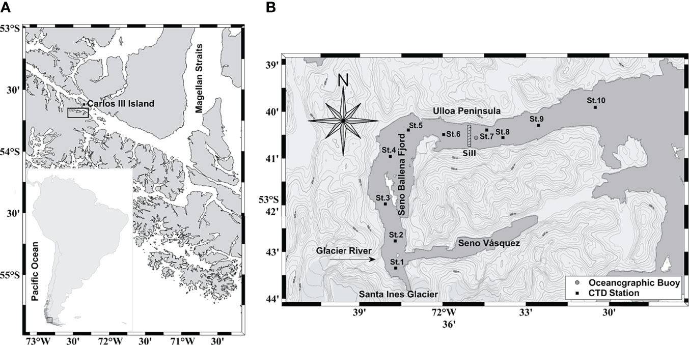
Figure 1 Map of the fjord region in southernmost Patagonia (A), showing Seno Ballena Fjord adjacent to Santa Inés glacier (B). The mooring was anchored adjacent to the sill (circle, South Patagonia Buoy: http://portal.goa-on.org/Explorer?action=oiw:fixed_platform:M_653:observations). Squares indicate synoptic stations sampled during three seasons (fall, winter, and spring).

Fjord-glacier systems are singular but diverse in their characteristics and thus likely also in their dynamics. Factors such as the hydrographic characteristics of the watershed, glacier dynamics, bathymetry, wind and sun orientation, latitude, location of the ice edge (e.g., glacier-terminating fjord, glacier edge on the coast or far from the shoreline) may be critical to understand the response of fjords to climate forcing. It has been suggested that the increase in air temperature and atmospheric pCO₂ in recent years may result in increased cold freshwater input from the glaciers (Bown et al., 2014), with a large potential to perturb the carbonate system speciation (Meire et al., 2015; Hopwood et al., 2020) and thus marine biota (Orr et al., 2005; Kurihara, 2008; Grear et al., 2017; Giesecke et al., 2019). Current projections of how changes in the ocean carbonate system may influence biological processes (i.e., photosynthesis and microbial respiration) in the future still remain speculative. Hydrological and biogeochemical information for Seno Ballena, a glacier-fjord system, will be relevant for explaining biological responses to coastal acidification interacting with other climate stressors (i.e., warming and reduced salinity due to increased freshwater flow). In this study, the main objective is to examine the carbonate system’s seasonal dynamics due to the influence of glacier meltwater and oceanic waters on the upper surface layer along the fjord. This study specifically presents the seasonal hydrography and time series of pCO₂, pH_T, and O₂ in the Seno Ballena glacier Fjord from austral fall through spring (March to December, 2018).

2 Materials and Methods

2.1 Study Area

Seno Ballena fjord is part of the Marine Protected Area Francisco Coloane, in the Strait of Magellan (53°42′S, 72°36′W; Frangópulos et al. (2007); Figure 1). It is 18 km long from the head, where the Santa Inés glacier is located, to the outside of the sill in the direction of Carlos III Island, Strait of Magellan (Figure 1). The lower (southwest) area of the fjord is approximately 9 km long and less than 1 km wide. A sill reaching a depth of 2–3 m from the surface during high tide is located 7 km from the glacier (Valle-Levinson et al., 2006). The bathymetry is highly variable from the inside to the outside of the fjord. Near the glacier depths are between 20 to 50 m, followed by a deeper area of 150 m up to the sill; past the sill depths of more than 200 m are found. This system is strongly influenced by freshwater input from (1) the melting of the glacial ice located at the head of the fjord; (2) a river of glacial origin; (3) melting snow of the adjacent mountains, that forms several small tributaries along the fjord (Supplementary Figure 1); and (4) high rainfall (4500–6000 mm y^-1; Meier et al., 2018). These hydrological processes are the primary controls of the stratification of the fjord, characterized by a thin (~10 m) surface layer of low-salinity water (24 - 28 S_p).

The fjord is within the Sub-Antarctic fjord and channel system of Patagonia (Figure 1), for which a strong influence of Modified Sub-Antarctic Waters mass (MSAAW) has been proposed (Supplementary Figure 2). This water mass occupies a significant fraction of the Strait of Magellan and Sub-Antarctic fjords, having practical salinity values (S_p) between 31 and 34 (Silva et al., 1998; Sievers et al., 2002; Valdenegro and Silva, 2003). When this water mass mixes with freshwater runoff from rivers and glaciers it forms estuarine waters, which are classified into three categories: the saline water of the estuary is more than 66% seawater (21-31 S_p); estuary-brackish water is 33-66% seawater (11-21 S_p); and freshwater in estuaries is less than 33% seawater (2-11 S_p) (Sievers and Silva, 2008). MSAAW has low dissolved silicate (DSi) compared to nitrate concentration. In contrast, given the geology of the drainage basin, the siliceous crystalline batholiths of Patagonia, the continental shelf waters of western Patagonia are characterized by high DSi, low nitrate, low alkalinity and low Ca²⁺ (Hervé et al., 2007; Torres et al., 2020).

2.2 Hydrographic Measurements

Three seasonal oceanographic cruises were conducted along the fjord in March (fall), August (winter), and December (spring), 2018. Five to ten stations along the main axis of the fjord were visited during each cruise (Figure 1). Hydrographic profiles (in situ temperature and salinity) were obtained using a CTD (SeaBird SBE model 19). The CTD salinity data in spring were not used due to CTD technical problems, and consequently salinity was determined from water samples taken at distinct depths (0, 5, 10, 25, and 50 m) and measured using a YSI-Pro30 probe at constant temperature previously calibrated with an IAPSO standard seawater (35 S_p); the nominal uncertainties on these measurements were ±1%. The water masses were identified by the mixing triangle method (Mamayev, 1975), using the information from the fall and winter campaigns to confirm the presence of MSAAW (Silva et al., 2009). Throughout practical salinity (PSS-78) is reported as S_p (UNESCO, I. 1981).

2.3 Water Samples and Analysis

Samples for the determination of carbonate chemistry parameters, inorganic nutrients and autotrophic biomass were taken at 5–8 stations, at 0, 5, 10, 25, and 50 m depths. Samples were also taken from glacier ice as well as river-glacier water and small freshwater tributaries along the fjord to determine freshwater end-members of salinity and alkalinity. Water samples were collected in 10 L Go-Flo bottles and stored in the dark at low temperature (< 7°C) in 250 mL gas-tight containers for the analysis of total alkalinity (A_T) and pH_T. Seawater samples for A_T analysis were poisoned with 50 μl of a saturated mercuric chloride solution (HgCl₂; Dickson et al., 2007). pH_T was analyzed soon after collection (<12 h), using purified m-cresol purple as an indicator at 25.0°C with an Ocean Optics STS-Vis (350 – 800 nm) spectrophotometer (Byrne et al., 1988). When possible, pH_T was also measured with an aquatrode probe (Metrohm TM) with a single point calibration (pH Tris buffer pH=8.089 at 25.0°C and salinity 35) (Dickson and Goyet, 1994). Mean differences from three replicate samples between methods were 0.01 pH units in the 28 - 31 salinity range (spectrophotometer and electrode pH). Tris buffer was made for salinity 35 whereas the field salinities ranged from 27.4 to 31.2. Nevertheless, we have determined empirically (using buffers at salinity 35 and 25, and this electrode) that the uncertainties in pH due to differences in salinity between buffer and sample is lower than 0.01 pH units. The performance (i.e., Nernstian slope) of the electrode was better than 99.8% of the theoretical value.

A_T analysis was performed with the automatic open-cell potentiometric titration method (Haraldsson et al., 1997). This technique allows A_T to be obtained quickly and very precisely with a small sample volume (~ 40 ml) by adding hydrochloric acid (0.05 M HCl; Merck Titrisol^®) in increasing volumes with a Dosimat 665. The reading was done with a combination Ross electrode (Orion 8102BN). The end-point was determined by the Gran method (Gran, 1952) according to Haraldsson et al. (1997). Each sample was analyzed twice and the average and standard deviation are reported. Seawater distributed by Dr. Andrew Dickson’s laboratory was used to verify the A_T estimates.

Filtered (0.7 µm glass fiber filters; Whatman GF/F) samples were frozen (-20°C) for analysis of soluble reactive phosphate (SRP), ${\text{NO}}_3^{-}$ and dissolved silicate (DSi), using the manual techniques recommended by Parsons et al. (1984). The inorganic nutrients and A_T were analyzed in the carbonate laboratory at the Centro de Investigación de Ecosistemas de la Patagonia (CIEP, Coyhaique). Chlorophyll-a concentration of seston larger than 0.7 μm was extracted with 90% acetone and measured using a fluorometer (Turner P700) following Parsons et al. (1984).

Estimates of in situ pH_T, pCO₂ and aragonite saturation state (Ω_Ar) were calculated using the chemical speciation model program CO₂SYS (Pierrot et al., 2006), using the dissociation constants (K₁ and K₂) estimated by Mehrbach et al. (1973), modified by Dickson and Millero (1987) for salinity = 20 - 40 and temperatures 2 - 35°C. Our values fit into these ranges of S_P and temperatures. We used the equilibrium constants for KHSO₄ determined by Dickson (1990) and those for Total Boron determined by Uppström (1974). The dissociation constants provided by Dickson and Millero (1987) have been shown to be consistent with results of previous studies carried out in the Chilean Patagonia fjords (Torres et al., 2011b; Alarcón et al., 2015; Vergara-Jara et al., 2019; Torres et al., 2020). Input data for CO₂SYS used T, S_P, A_T, pH_T@25°C and nutrients (SRP and DSi) (Kim and Lee, 2009). We measured only two parameters in discrete samples (pH_T and A_T) and two in the in situ sampling (pH_T and pCO₂, see section 2.5); therefore we cannot estimate the internal consistency of the measured carbonate system parameters. Organic matter (organic acids, fulvic and humic acids) could be a significant source of non-carbonate alkalinity, produced during decomposition of organic matter in sediments carried away by inland waters (Lukawska-Matuszewska, 2016). Therefore, care was taken to interpret calculated carbonate system parameters since they may result in overestimation of DIC and pCO₂. Organic alkalinity does not play an important role in this system, given the low average contribution to the total alkalinity of the freshwater end-members (5.8 ± 16.0 μmol kg^-1).

2.4 Water Mass Distribution Analysis

To quantify the relative contributions of freshwater from the Santa Ines glacier and adjacent river-glacier from the oceanic-type water mass (estuarine-brackish: MSAAW), an optimum multiparameter (OMP) analysis was performed, which uses a simple model of linear mixing to calculate the fraction of the source-water types. Two conditions are taken into account to apply the method: (1) all the calculated fractions are positive and (2) the sum of all the fractions is close to 100% (conservation of mass). In our analysis, we found that only two water masses were not sufficient to reproduce the properties of the samples. Thus, we assume mixing that involves 3 water masses: (1) near-surface and (2) deep inner fjord water masses, whose property definitions are determined from the average of a set of observations made during seasonal synoptic sampling, and (3) the oceanic water mass (MSSAW) that has traditionally been identified for this study area (Sievers and Silva, 2008; Silva et al., 2009).

To characterize the inner fjord water masses, property-property diagrams were made of the observations of salinity, temperature, A_T and nutrients to select values that represent the source water types. The observations used for the Inner Surface Source Water (ISSW) were from the surface sampling station closest to the glacier, to represent the properties of the freshwater from the glacier-ice and river-glacier. The observations used to characterize the Inner Bottom Source Water (IBSW) were from sampling stations 2 at 50 m depth (2 km from the glacier). The oceanic water mass that enters this Sub-Antarctic zone is the Sub-Antarctic water mass (SAAW), which is modified within the Strait of Magellan by mixing with continental freshwater (runoff from glaciers and rivers), forming MSAAW and is found from the surface to 150 m depth. The properties of the MSAAW were established based on reported information (Sarmiento et al., 2004; Sievers and Silva, 2008; Silva et al., 2009; Llanillo et al., 2012; Torres et al., 2014; Forcén-Vázquez et al., 2021). The strong salinity and alkalinity relationship reported for the Patagonian archipelago interior sea (41–56°S: Torres et al., 2011a; Torres et al., 2020) makes it possible to calculate alkalinity of the MSAAW using the equation: A_Tsal (μmol kg^-1) = 66.4 × Salinity + 1.1, (R² = 0.93, n=81; Figure 2; Supplementary Table 1). The regression is close to the equations reported for the Sub-Antarctic region A_T (μmol kg⁻¹) = 61.9 × Salinity + 151 and A_T (μmol kg⁻¹) = 61.8 × Salinity + 145; Torres et al. (2011b) (Figure 2). The intercept (1.1 μmol kg⁻¹) is a reasonable estimate of the freshwater end-members (glacier-ice and small tributaries along the fjord) with the value mean (A_T of 5.8 ± 16.0 μmol kg⁻¹; n = 7, salinity 0.0 ± 0.1 S_P).

FIGURE 2

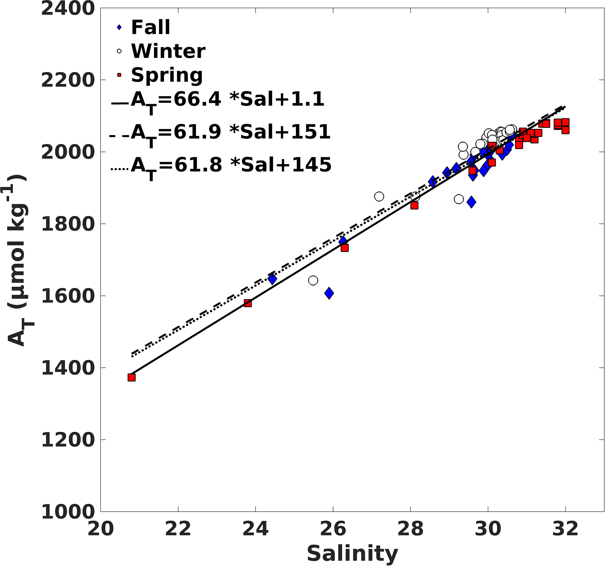
Figure 2 Relationship between A_T and salinity from Seno Ballena Fjord transect data (fall-winter-spring austral, 2018). The line represents the regression obtained for Seno Ballena fjord in this study and the dashed lines are the regression obtained at the eastern portion of the Patagonia archipelago (from surface water) inner sea (50–53°S; Torres et al., 2011b).

The water masses proposed in this analysis have ranges of values, thus 5 source types of water (SWT) were used as described in Table 1 (ISSW₁, ISSW_2, ISBW₁, MSAAW_1, and MSAAW₂). The weights for each variable were chosen taking into account the extent of their conservative behavior and their spatial and temporal variability (S_p = 25, Temp = 25, DSi = 5, NO₃ = 5, A_T = 25). The salinity and A_T data were assigned relatively high weights, because they are conservative in the temporal and spatial scales considered here. Temperature and nutrients were assigned lower weights; temperature due to its high seasonal variability caused by heating and cooling and nutrients due to the changes caused by biological processes. The linear system of mixing equations, that were solved using the classic OMP analysis (MATLAB - version 1.2.0.0; Karstensen, 2013), are the following:

$\begin{array}{ll}{x}_a{T}_a+x_b{T}_b+x_c{T}_c+x_d{T}_d+x_e{T}_e=T_{obs}+R_T& \text{(1a)}\end{array}$

$\begin{array}{ll}{x}_a{S}_a+x_b{S}_b+x_c{S}_c+x_d{S}_d+x_e{S}_e=S_{obs}+R_S& \text{(1b)}\end{array}$

$\begin{array}{ll}{x}_a{A}_{Ta}+x_b{A}_{Tb}+x_c{A}_{Tc}+x_d{A}_{Td}+x_e{A}_{Te}=A_{Tobs}+R_{A_T}& \text{(1c)}\end{array}$

$\begin{array}{ll}{x}_{a}DS{i}_a+x_{b}DS{i}_b+x_{c}DS{i}_c+x_{d}DS{i}_d+x_{e}DS{i}_e=DS{i}_{obs}+R_{DSi}& \text{(1d)}\end{array}$

$\begin{array}{ll}{x}_{a}N{O}_{3a}+x_{b}N{O}_{3b}+x_{c}N{O}_{3c}+x_{d}N{O}_{3d}+x_{e}N{O}_{3e}=N{O}_{obs}+R_{N{O}_3}& \text{(1e)}\end{array}$

$\begin{array}{ll}{x}_a+ x_b+x_c+x_d+x_e= 1+ R_{\Sigma }& \text{(1f)}\end{array}$

TABLE 1

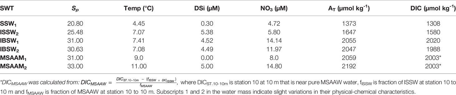
Table 1 Properties of ISSW (Inner Surface Source Water), IBSW (Inner Bottom Source Water), and MSAAW (Modified Sub-Antarctic Water) for the OMP and time-series water mass model.

where T_obs, S_obs, A_Tobs, DSi_obs and NO_3obs are the values observed during the seasonal sampling and the R_∑ are their respective residuals. The values T_i, S_i, A_Ti, DSi_i and NO_i (i = a, b, c, d and e) define the fixed parameter values of the five source-water types, that define the three water masses (ISSW, IBSW and MSAAW). The five tracers plus conservation of mass leaves little redundancy for five water types (Karstensen and Tomczak, 1998), since we need to include the fifth water type (IBSW) as it is distinctly different than the other four. x_i is the fraction for each data point. Equation (1f) is the mass conservation constraint.

2.5 pH-pCO₂ Mooring Sensors

High-resolution measurements of pCO₂ and pH_T were recorded in situ using the autonomous submersible SAMI-CO₂ and SAMI-pH sensors (Sunburst Sensors, LLC) (DeGrandpre et al., 1995), temperature and conductivity using SBE37 sensors and dissolved oxygen (DO) using an Aanderaa 5331A sensor. SAMI-CO₂ measures the partial pressure of carbon dioxide (pCO₂) in water from 200 to 1000 μatm (precision <1 μatm, accuracy ~10 µatm), while SAMI-pH measures pH_T on total proton concentration scale in the marine pH range of 7 - 9 for salinity ranges 25 - 40 S_P (Clayton and Byrne, 1993). The two sensors use a high-precision colorimetric reagent method (http://www.sunburstsensors.com/).

The factory SAMI-CO₂ calibration, based on coincident measurements of pCO₂ using gas-equilibration with infrared detection, was used for this study. The SAMI-pH is not factory calibrated but was validated using a Tris buffer at 25°C (accuracy and precision ~ ± 0.003). All of the sensors were placed at 10 ± 1 m and mounted on one single steel frame with the sensors’ water intakes in the same vertical position. The sensors were deployed in the lower part of the pycnocline on the outer side of the sill (Figure 1). Mooring measurements started early in austral fall (March, 2018) and ended in austral spring (December, 2018). All sensors recorded data every 4 hours. Discrete samples of the three seasonal oceanographic cruises (March, August, and December 2018) were used for data quality control.

The SAMI-pH and A_Tsal data were used to compute the additional carbonate system parameters because this pair was shown to yield good accuracy (Cullison Gray et al., 2011). The total alkalinity (A_Tsal) values derived from salinity carry an error of 42 μmol kg^-1. This error is estimated from the values of the A_Tsal time series for the days that coincide with the seasonal A_T-measured samples measured in fall, winter, and spring. For this calculation, A_T-measured data were collected from a sampling station near the mooring at a depth of 10 m.

All inorganic carbon parameters were calculated with CO₂SYS software (Pierrot et al., 2006) as described above (see item 2.3). Nutrient data were not included in the computations due to the lack of continuous measurements during the study. The calculated pCO₂ changed by ~ 1.0 μatm when the highest observed levels of SRP (1.76 μM) and DSi (5.47 μM) were included in CO₂SYS.

2.6 CO₂ Flux Determination

The air-sea CO₂ flux was determined using the diffusive boundary layer model, through the volumetric flux equation expressed in terms of CO₂ partial pressure:

$\begin{array}{ll}F=K \times K_O\left(pC{O}_{2W}-pC{O}_{2a}\right)& (2)\end{array}$

where F is the air-sea flux in units of moles area⁻¹ time⁻¹, K is the gas transfer velocity in units of length time⁻¹ (Wanninkhof, 1992), K_O is the solubility coefficient of CO₂ (mol m⁻³ atm⁻¹), estimated from in situ salinity and temperature according to Weiss (1974) and the pCO_2W – pCO_2a is the difference between the air and sea surface pCO₂ values in µatm. Results with positive values indicate that there is a flux from sea to atmosphere. The gas transfer velocity of CO₂ was calculated using the revised relationship recommended by Wanninkhof (2014):

$\begin{array}{ll}K =0.251 \langle U^2\rangle {\left(\frac{Sc}{660}\right)}^{-0.5} & (3)\end{array}$

where <U²> is the mean squared wind speed (m s^-1). The wind speed data were obtained from a meteorological station near the study area (Chile Meteorological Directorate, Alberto Hurtado School station, coordinates: -53.16694°S, -70.94528°W).

The updated Wanninkhof (2014) parameterization was used in the study of the gas transfer rate estimation in Seno Ballena fjord because it considers the most recent advances in the quantification of the input parameters, improvements in the wind speed products and it provides good estimates for most insoluble gases in intermediate wind speed ranges (3 - 15 m s¹). The mean wind speed in Seno Ballena Fjord was 4.04 m s^-1 during the study period (range of 3.73 to 6.04 m s^-1). Sc is the Schmidt number which accounts for the difference in molecular diffusivity between gases, with the leading coefficient updated for seawater (35 S_P) and freshwater (0 S_P) at temperatures ranging from -2 to 40°C by Wanninkhof (2014). Sc is calculated using:

$\begin{array}{ll}Sc=A+ B_t+ C_t+D_t+E_t& (4)\end{array}$

where t is temperature (°C) and A, B, C, D, and E are fitting coefficients (Wanninkhof, 2014).

The formula described by Dickson et al., (2007) was used to calculate the atmospheric pCO₂ values in humid air and the water vapor pressure values:

$\begin{array}{ll}pC{O}_{2a}=pC{O}_2\left(dry-air\right) \times \left(1-P_W\right)& (5)\end{array}$

where pCO₂ (dry - air) is the air pressure at sea level taken from the Earth System Research Laboratory database (National Oceanic and Atmospheric Administration Marine Boundary Layer Reference 53.1 to 17.5°S; www.esrl.noaa.gov/gmd/ccgg/mbl/data.php), interpolated for the year 2018 and corrected with local barometric pressure. These values assume clean marine air, and therefore a possible error is created due to terrestrial effects on pCO₂, mainly of the export of organic and inorganic carbon from land runoff, rivers and glaciers (Lafon et al., 2014). The error is not readily quantifiable because no regional pCO₂ data are available. P_w is the equilibrium water vapor for the in situ temperature (°C) and salinity (S_P) (Forstner and Gnaiger, 1983).

2.7 Temperature Effect on pCO₂

Temperature changes affect the partial pressure of seawater due to its solubility. For this reason, the values of the pCO₂ time series were adjusted to a mean temperature, using the equation of Takahashi et al. (2009) (Eqn. 6). The temperature coefficient (0.0459) for cold (-1.8 to 10°C) and less saline (30 < S_P < 35) water (Ericson et al., 2018) was used, as these ranges match the observed salinity and temperature ranges of the Seno Ballena fjord.

$\begin{array}{ll}npC{O}_{2 }= pC{O}_{2obs}\times exp\left[0.0459 \times \left(T_{ave}-T_{obs}\right)\right]& (6)\end{array}$

where pCO_2obs are the values of the pCO₂ time series. The mean temperature during the study period (March to December 2018; T_ave) was 7.67°C, and T_obs is the measured temperature in degrees Celsius. This equation makes it possible to determine if changes in pCO₂ in spring are related to phytoplankton bloom events rather than just to temperature changes.

2.8 Apparent Oxygen Utilization

Apparent oxygen utilization is calculated to estimate the effect of biology on oxygen concentrations, eliminating the effect of temperature and solubility. It was calculated using the following equation:

$\begin{array}{ll}AOU=D{O}_{sat}-DO& (7)\end{array}$

This equation represents the change in oxygen since a mass of water was last in contact with the atmosphere, assuming that the oxygen concentration at the surface was at equilibrium with the atmosphere (DO_sat). DO is the measured dissolved O₂. AOU estimates biological processes; positive values indicate aerobic remineralization processes, which consume DO, and negative values indicate photosynthetic processes, which produce DO (Pytkowicx, 1971; Ito et al., 2004; Jackson et al., 2021).

2.9 Mixing Model

We use a simplified mixing model to determine the effects of mixing versus photosynthesis/respiration in the time series. Because we have no nutrient measurements at the mooring, we use only salinity and temperature and thus can only use three end-members. The choice of the end-members was based on a T-S diagram (Supplementary Figure 3). ISSW₁, IBSW₂, and MSAAW₁, define a triangle that best contains the mooring data and were selected to estimate the fractions of each type of water at the mooring at each moment. Table 1 shows the values of end-members of temperature and salinity for each water type.

Equations (8a), (8b), and (8c) were used to determine the mixing ratios f. Equations (8d) and (8e) were used to calculate the DIC and A_T that would result from mixing these three water masses.

$\begin{array}{ll}1= f_{ISSW}+ f_{IBSW}+ f_{MSAAW }& \text{(8a)}\end{array}$

$\begin{array}{ll}{T}_{mix}=f_{ISSW} \times T_{ISSW}+f_{IBSW} \times T_{IBSW}+ f_{MSAAW} \times T_{MSAAW}& \text{(8b)}\end{array}$

$\begin{array}{ll}{S}_{mix}=f_{ISSW} \times S_{ISSW}+f_{IBSW} \times S_{IBSW}+ f_{MSAAW} \times S_{MSAAW}& \text{(8c)}\end{array}$

$\begin{array}{ll}DI{C}_{mix}=f_{ISSW} \times DI{C}_{ISSW}+f_{IBSW} \times DI{C}_{IBSW}+ f_{MSAAW} \times DI{C}_{MSAAW}& \text{(8d)}\end{array}$

$\begin{array}{ll}{A}_{Tmix}=f_{ISSW} \times A_{TISSW}+f_{IBSW} \times A_{TIBSW}+ f_{MSAAW} \times A_{TMSAAW}& \text{(8e)}\end{array}$

where f is the end-member mixing ratio. T°C, S_p, DIC, and A_T are temperature, salinity, dissolved inorganic carbonate, and total alkalinity for each end-member (Table 1).

The pCO₂ due to mixing was calculated from the following equation:

$\begin{array}{ll}pC{O}_{2mix}= f\left(DI{C}_{mix}, A_{Tmix}, S_{mix}, T_{mix}\right)& (9)\end{array}$

where the term f (DIC_mix, A_Tmix, S_mix, T_mix) is the calculation of pCO₂ using DIC, A_T, S_p and T°C to the CO₂SYS program (Pierrot et al., 2006).

2.10 1-D Biochemical Mass Balance Model

A simple 1-D mass budget model determined the contribution of biological processes, physical mixing, air-sea CO₂ exchange, and thermodynamics to pCO₂ variability. The changes in pCO₂ due to dissolution/formation of CaCO₃ and salinity are omitted.

The daily changes in the pCO₂ were estimated as previously carried out by various authors (Chierici et al., 2006; Xue et al., 2016; Fransson et al., 2017; Li et al., 2018; Gac et al., 2021). Changes in pCO₂ (ΔpCO₂) are driven by changes in temperature (ΔpCO_2tem), air-sea CO₂ exchange (ΔpCO_2gas), mixing (ΔpCO_2mix), and biological activity (ΔpCO_2bio). ΔpCO₂ and ΔDIC are calculated using:

$$\Delta pC{O}_2={\left(pC{O}_2\right)}_{n+1}-{\left(pC{O}_2\right)}_n$$

$\begin{array}{ll}=\Delta pC{O}_{2tem}+\Delta pC{O}_{2gas}+\Delta pC{O}_{2mix}+\Delta pC{O}_{2bio}& \text{(10a)}\end{array}$

$\begin{array}{ll}\Delta DIC={\left(DIC\right)}_{n+1}-{\left(DIC\right)}_n=\Delta DI{C}_{gas}+\Delta DI{C}_{mix}+\Delta DI{C}_{bio}& \text{(10b)}\end{array}$

where Δ is the change in parameters between times (begin) t_n and t_n+1 (end) are the difference between the daily value at t_n+1 minus the daily value a t_n.

2.10.1 The Effect of Thermal Changes

Temperature changes affect the dynamics of the pCO₂ but not the DIC of the water. Therefore, the thermal effect on ΔpCO_2tem was determined according to the equation (similar to Eqn 6 above; Takahashi et al., 1993)

$\begin{array}{ll}\Delta pC{O}_{2tem}= {\left(pC{O}_2\right)}_n \times exp\left(0.0459 \times \Delta T\right)-{\left(pC{O}_2\right)}_n& (11)\end{array}$

where (pCO₂)_n is pCO₂ at time 1, ΔT is the temperature difference between time t_n+1 and t_n.

2.10.2 The Effect of Air-Sea Gas Exchange

Air-sea CO₂ exchange affects the dynamics of DIC and pCO₂ but not the A_T. Therefore, the pCO₂ changes due to the air-sea CO₂ exchange (ΔpCO_2gas) are calculated using:

$\begin{array}{ll}\Delta DI{C}_{gas}= F_{gas}\times \left(t_{n+1 }-t_n\right)/ \left(\rho \times d\right)& \text{(12a)}\end{array}$

where F_gas is the air-sea CO₂ flux (see Section “Air-sea CO₂ exchanges”) t_{n+1 -} t_n is the number of days between two measurements, ρ is the seawater density (kg m^–3) calculated from the TEOS-10 calculations (McDougall et al., 2011), and d is the mixed layer depth taken to be 10 m, the depth of the mooring.

$\begin{array}{ll}{\left(DI{C}_{n+1}\right)}_{gas}= DI{C}_n+ \Delta DI{C}_{gas}& \text{(12b)}\end{array}$

$\begin{array}{ll}\Delta pC{O}_{2gas}=f\left({\left(DI{C}_{n+1}\right)}_{gas}, A_{Tn}, S_n, T_n\right)-{\left(pC{O}_2\right)}_n& \text{(12c)}\end{array}$

where (DIC_n+1)_gas is DIC predicted for time t_n+1 based solely on air-sea CO₂ exchange. The term f ((DIC_{n+ 1})_gas, A_Tn, S_n T_n) is the calculation of pCO₂ using DIC, A_T, S, and T to the CO₂SYS program (Pierrot et al., 2006).

2.10.3 The Effect of Water Mass Changes

To determine the changes in pCO₂ due to mixing the pCO₂ was calculated from DIC_mix and A_Tmix derived from the fraction of each water mass using equations:

$\begin{array}{ll}\Delta DI{C}_{mix}= DI{C}_{mix\left(n+1\right)}-DI{C}_{mix\left(n\right)}& \text{(13a)}\end{array}$

$\begin{array}{ll}\Delta A_{Tmix}= A_{Tmix\left(n+1\right)}-A_{Tmix\left(n\right)}& \text{(13b)}\end{array}$

where ΔDIC_mix and ΔA_Tmix are DIC and A_T of mixing (see Section “Mixing model”) t_{n+1 -} t_n is the number of days between two measurements DIC_mix(n+1) and A_Tmix(n+1) are predicted DIC and A_T based solely on the mixing.

$\begin{array}{ll}\Delta pC{O}_{2mix}=f\left({\left(DI{C}_{n+1}\right)}_{mix}, {\left(A_{Tn+1}\right)}_{mix}, S_{n+1}, T_{n+1}\right)-{\left(pC{O}_2\right)}_n& \text{(13e)}\end{array}$

where f ((DIC_n+1)_mix, (A_Tn+1)_mix, S_n+1, T_n+1) is the calculation of pCO₂ using DIC, A_T, S and T to the CO₂SYS program (Pierrot et al., 2006).

2.10.4 The Effect of Biological Processes

The biological effect on pCO₂ is estimated as the remainder in the change of DIC.

$\begin{array}{ll}\Delta DI{C}_{bio}= \Delta DIC-\left(\Delta DI{C}_{gas}+\Delta DI{C}_{mix}\right)& \text{(14a)}\end{array}$

$\begin{array}{ll}{\left(DI{C}_{n+1}\right)}_{bio}= DI{C}_n+ \Delta DI{C}_{bio}& \text{(14b)}\end{array}$

$\begin{array}{ll}\Delta pC{O}_{2bio}=f\left({\left(DI{C}_{n+1}\right)}_{bio}, A_{Tn}, S_n, T_n\right)-{\left(pC{O}_2\right)}_n& \text{(14c)}\end{array}$

where (DIC_n+1)_bio is the predicted DIC based solely on the biological factor. f ((DIC_n+1)_bio, A_Tn, S_n, T_n) is the calculation of pCO₂ using DIC, A_T, S, and T in the CO₂SYS program (Pierrot et al., 2006).

3 Results

3.1 Hydrography and Nutrients

The hydrography of the Seno Ballena fjord was modulated by the seasonal input of freshwater from glacier meltwater, the glacial river located at the head of the fjord, and the small tributaries along the fjord. The influence of the MSAAW was also evident given the range of salinities observed (24 - 31); the fjord water is estuarine-brackish (33 - 66% seawater). The contribution of freshwater from the Inner Surface Estuarine Water (ISSW) near the glacier is distributed from the head of the fjord towards the outside of the sill near the surface, with smaller fractions outside of the sill (Figures 3A–C). In fall and spring, the deep layer contained not only MSAAW, but also another type of water (IBSW) near the glacier, that is cold and nutrient-rich (Figures 3D, F). In fall the surface ISSW was mixed deep inside the fjord. Finally, the MSAAW dominated the deep layer of the inner fjord, which confirms that this estuarine-brackish water enters the fjord (Figures 3G–I). The MSAAW contribution was greater in winter (from 5 - 50 m depth). This mixed water mass was associated with a strong vertical density gradient (σ_t range from surface to depth: fall = 19.20 - 23.97; winter = 20.18 - 23.98; spring = 17.17 - 22.82).

FIGURE 3

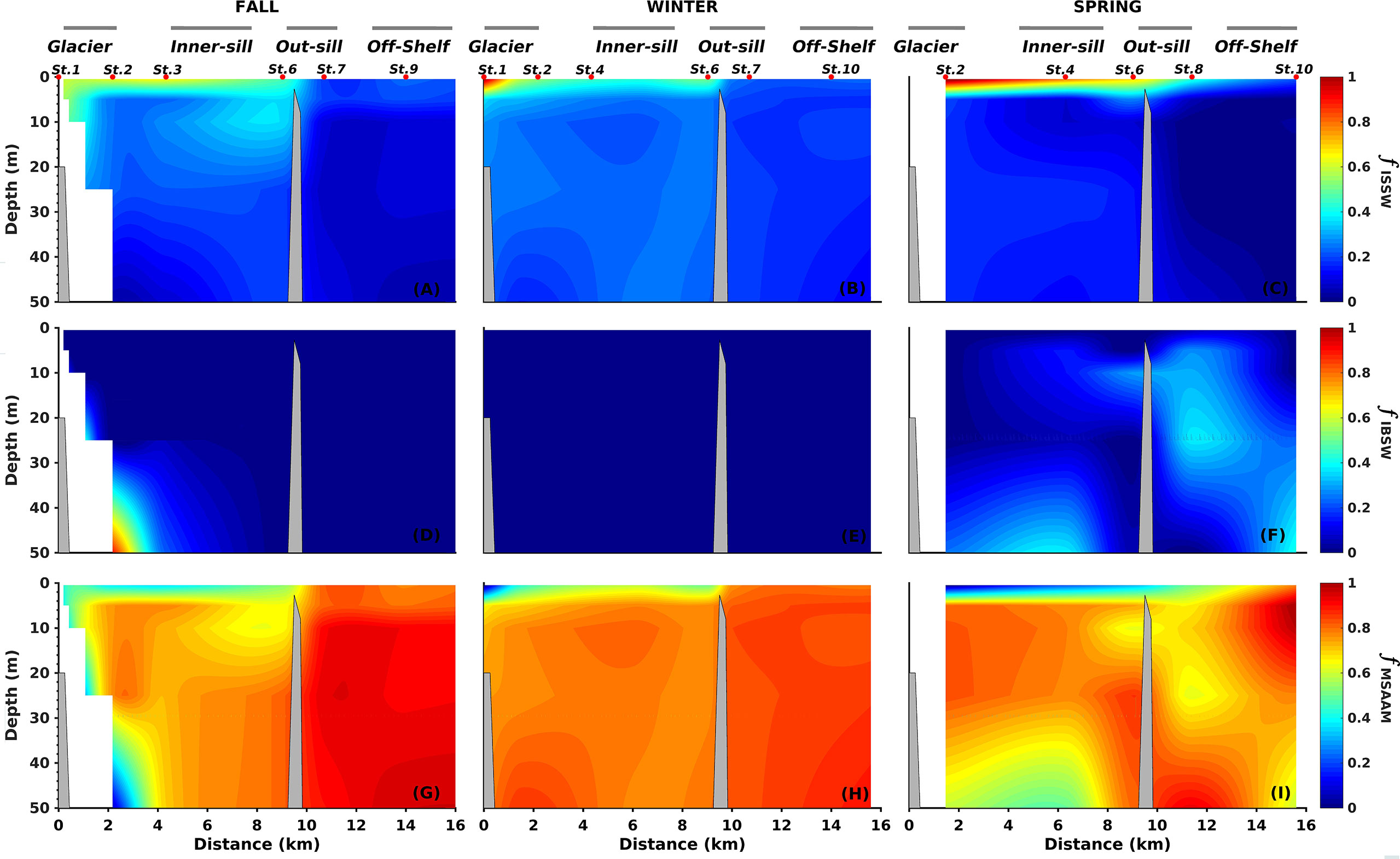
Figure 3 Fraction (f) of Inner Surface Source Water (ISSW; A–C), Inner Bottom Source Water (IBSW; D–F), Modified Subantarctic Water (MSAAW; G–I) along Seno Ballena Fjord during the seasonal sampling. The fractions were estimated using OMP analysis (Optimum Multiparameter; MATLAB - version 1.2.0.0; Karstensen, 2013).

We divided the fjord area into three zones (inner sill, outer sill, and off-shelf), based on stratification and mixing conditions. In the inner sill region, the 0 - 10 m surface layer showed low salinity, between S_P = 27.4 to 28.6, over a deeper layer with S_P ranging from 30.2 to 31.2 (Figures 4A–C). Salinity varied also with the season, showing high salinity in winter (range from surface to depth: S_P = 28.6 – 30.3) and low salinity in spring (range from surface to depth S_P = 27.4 – 31.2); the latter modulated by the input of glacier meltwater (Figures 4–C).

FIGURE 4

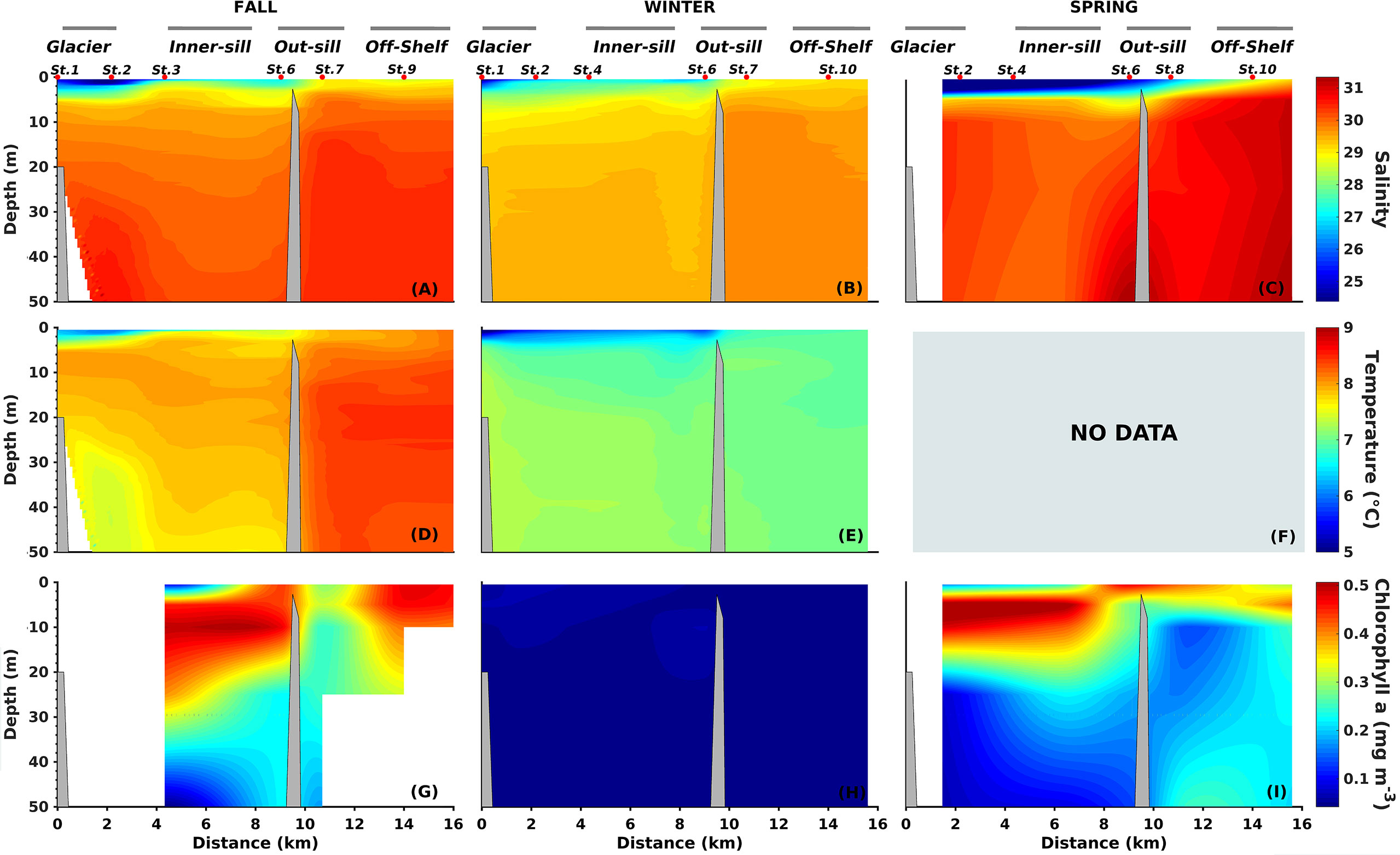
Figure 4 Vertical distribution of Salinity (A–C), Temperature (D, E), and Vertical distribution of Chlorophyll-a (G–I) along the Seno Ballena Fjord transect, during austral fall, winter, and spring 2018. Red markers correspond to synoptic sampling stations and grey horizontal lines indicate the extent of each section of the fjord (F) The CTD temperature data in spring is not available.

The water column had a thermal inversion and weak temperature variation in the inner sill region during fall and winter, with an increase of 0.7°C from the surface to the deep layer (Figures 4D, E). There were high temperature values in the fall (range from surface to depth 7.2 – 7.7°C) and low-temperature values in winter (range from surface to depth 6.4 – 7.3°C).

The stratification was much shallower in fall and spring and practically disappeared in winter in the outer sill section (Figure 4), coincident with a more significant influence of the oceanic water and lower influence of freshwater (S_P between 28.6 and 31.3 in the surface and deep layers, respectively; Figures 3, 4). Mixed conditions were observed in the off-shelf region, with a high S_P of 30.5 throughout the water column (Figures 4A–C). The fall and winter data showed a very stable surface layer (>10 m) in the water column of the inner section, with Brunt-Väisälä frequency squared values of 10 - 30x10^-3 s^-2 compared to outer sections (< 10x10^-3 s^-2; Supplementary Figure 4).

Nutrient concentrations (SRP, ${\text{NO}}_3^{-}$, and DSi) had a clear spatial variability from the inner to the outer sections of the fjord (Figure 5; Table 2). Surface ${\text{NO}}_3^{-}$ showed low to medium concentrations along the fjord, ranging from 5.7 – 7.4 μM (inner sill) to 9.3 μM (off-shelf), and in the deep layer ${\text{NO}}_3^{-}$ concentrations ranged from 6.2 – 11.1 μM (inner sill) to 11.5 μM (off-shelf) (Figure 5). Most of the time DSi concentrations were below 5 μM throughout the water column along the fjord. DSi concentrations were very low in the surface water along the fjord in fall and spring, with a range from 0.2 μM (off-shelf) to 2.7 μM (inner sill), increasing up to 4.6 μM in the deep layer in the inner sill region. During winter, DSi values increased up to 5.5 μM, especially in the middle and inner sections of the fjord (Figure 5, Table 2). SRP concentrations were more homogeneously distributed throughout the water column with a range from 0.6 to 1.3 μM, with the highest concentrations in the inner section below 10 m during spring and fall (Figure 5; Table 2). ${\text{NO}}_3^{-}$ was strongly correlated with SRP in fall (R² = 0.9; n=28; p< 0.001) and spring (R² = 0.6; n=25; p< 0.001). N:P fluctuated between 7.2 in fall and 6.9 in spring, with lower ratios than the expected Redfield N:P ratio (16:1). DSi:N ratios were low in fall (0.5), winter (0.1), and spring (0.2) during the hydrographic cruises. These values are consistent with the values of 0.2 - 0.5 recorded in this fjord during spring by Torres et al. (2011a).

FIGURE 5

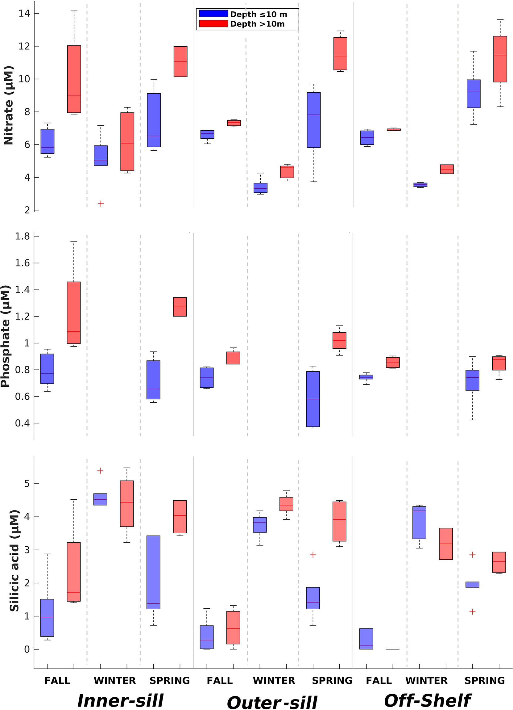
Figure 5 Median concentrations of nitrate, orthophosphate (SRP), and silicic acid (DSi) along the Seno Ballena Fjord during austral fall, winter, and spring (seasonal cruises 2018). Box-plots show the 25^th–75th quartiles of the data at each section; the lines show the maximum and minimum values; the red cross shows outlier values.

TABLE 2

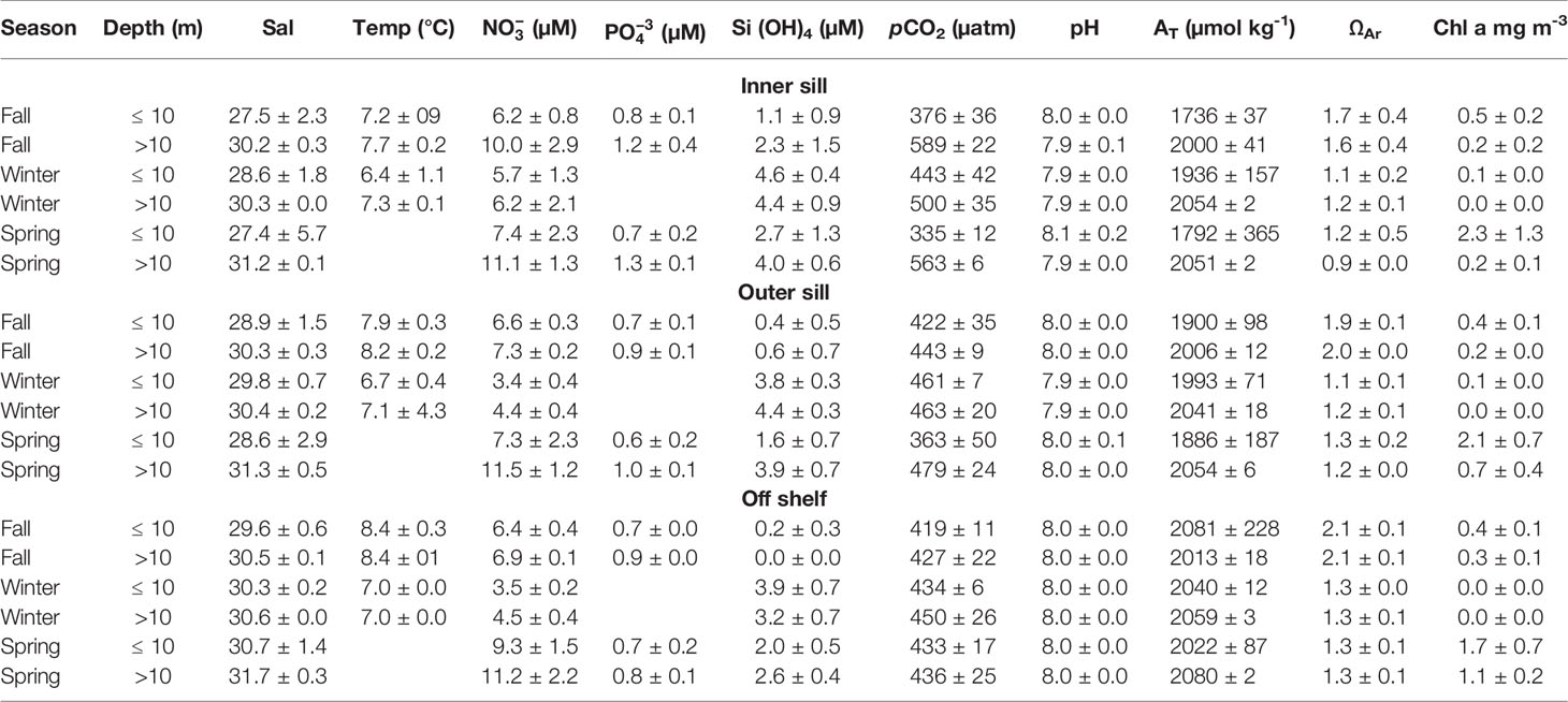
Table 2 Statistical descriptors of physical, chemical, and biological variables along Seno Ballena Fjord obtained during March (fall), August (winter), and December (spring) 2018 during three hydrographic cruises (mean ± 1 SD).

3.2 Carbonate Parameters From Hydrography Cruises

Low pCO₂ values were observed in the upper 10 m layer during the fall and spring cruises (< 400 μatm) in the inner fjord section; whereas, higher mean values were seen during winter (Table 2). Below the 10 m surface layer, pCO₂ values were much higher close to the glacier, 500 to 589 μatm (Figures 6A–C; Table 2). Mean pH values of 8.0 and 7.9 were observed in the inner section of the fjord in the upper 10 m layer and below 10 m depth, respectively, while pH for the outer sill was more homogeneous, with a mean value of 8.0 (SD=0.017) (Figures 6D–F; Table 2). The lowest pH values were observed below 10 m in the inner sections of the fjord and for most seasons were coincident with the highest pCO₂ values (Figure 6). High surface Chl-a was observed during spring in the upper layer in the whole transect, ranging from 2.3 (inner sill section) to 1.7 mg m^-3 (outer sill section) (Figure 4). These high Chl-a biomass was associated with high pH values (R² = 0.48; n=7; p<0.001) (Figures 4, 6, respectively).

FIGURE 6

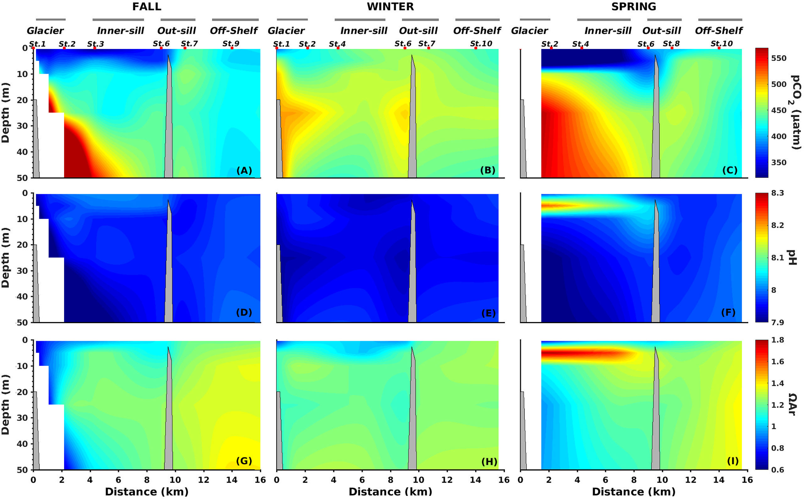
Figure 6 Vertical distributions of the partial pressure of CO₂ (pCO₂) (A–C), pH_T (D–F), and aragonite saturation state (Ω_Ar) (G–I) along the Seno Ballena Fjord transect, during austral fall, winter and spring, 2018. Red markers correspond to synoptic sampling stations and grey horizontal lines indicate the extent of each section of the fjord.

The A_T was low in the surface layer (< 10 m), coincident with low-salinity waters in the inner section, with seasonal mean values of 1736 to 1993 μmol kg^-1 (Table 2), associated with low values of Ω_Ar in the surface (R² = 0.42 n=50; p<0.001) (Figures 6G–I). Values of A_T were over 2000 μmol kg^-1 in the inner section of the fjord below the 10 m layer. The maximum Ω_Ar and A_T values were recorded in the off-shelf sections (2.1 and 2081 μmol kg^-1, respectively). These results indicate that during all seasons, freshwater inputs from the melting glacier and the glacial river were low in alkalinity (5.82 μmol kg^-1), whereas MSAAW was high in alkalinity (2081 μmol kg^-1).

3.3 Parameters From Mooring Sensors

The sea surface temperature values (outer sill section) also showed low seasonal variability, with amplitude not greater than 2°C. High values were recorded in fall with a mean of 8.2 ± 0.32°C (range 7.8 – 8.6°C) and low values were recorded in spring with a mean of 7.2 ± 0.22°C (range 6.6 – 7.7°C) (Figure 7; Supplementary Table 3). The S_P values recorded at the mooring showed a range from 29.8 to 30.5 with high values occurring in fall; whereas, minimum S_P occurred in spring (Figure 7). The salinity was above 28 throughout most of the studied seasons but presented a clear low amplitude seasonality (S_P <1.5) (Figure 7). The seasonal variability of T and S_P is related to the variable contributions of the different water masses of the fjord, with minor contribution of ISSW (0.04 - 0.23) compared to IBSW (0.05- 0.97) and MSAAW (0.01 - 0.85) at the mooring (Figure 8). MSAAW dominated the water masses during the fall; whereas, IBSW dominated during the spring. During the spring season, we observed at the end of October, an event during which the contribution of MSAAW (0.51) and IBSW (0.45) was more similar coinciding with a noticeable change in T and S_P, with respect to the values observed when a larger fraction of IBSW or MSAAW is recorded.

FIGURE 7

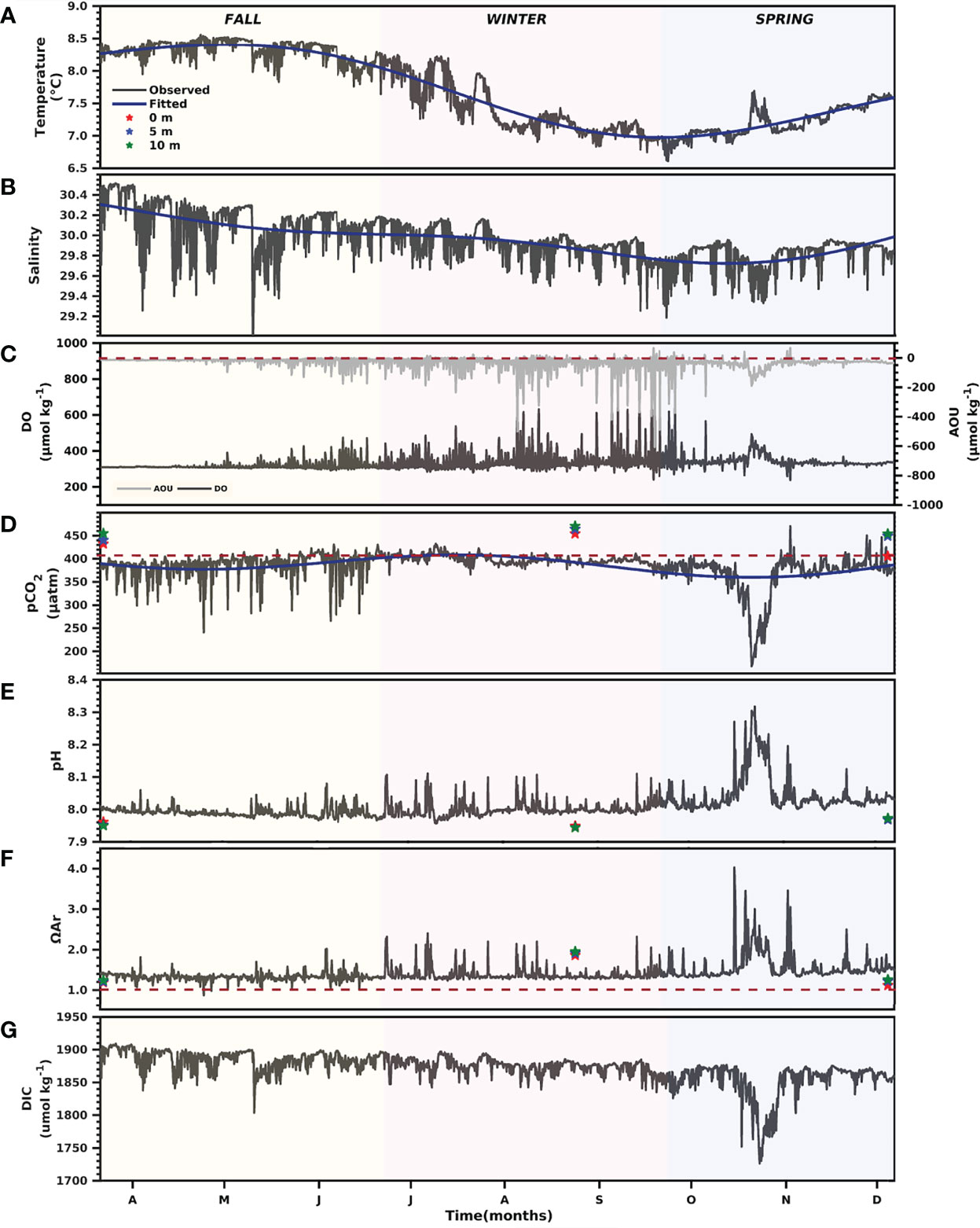
Figure 7 Seasonal dynamics of the primary measured parameters at the Seno Ballena mooring (Figures 1). Time-series of Temperature (A), Salinity (B), Oxygen and AOU (C), pCO₂ (D), pH (E), Aragonite saturation state (F) and dissolved in organic carbon (DIC) (G) from March to December 2018. The red dashed lines in (C) show the limit between positive values that indicate aerobic remineralization processes and negative values that indicate photosynthetic process, (D) shows the atmospheric value (mean 405 ± 1 uatm), (F) shows an aragonite saturation threshold of 1.

FIGURE 8

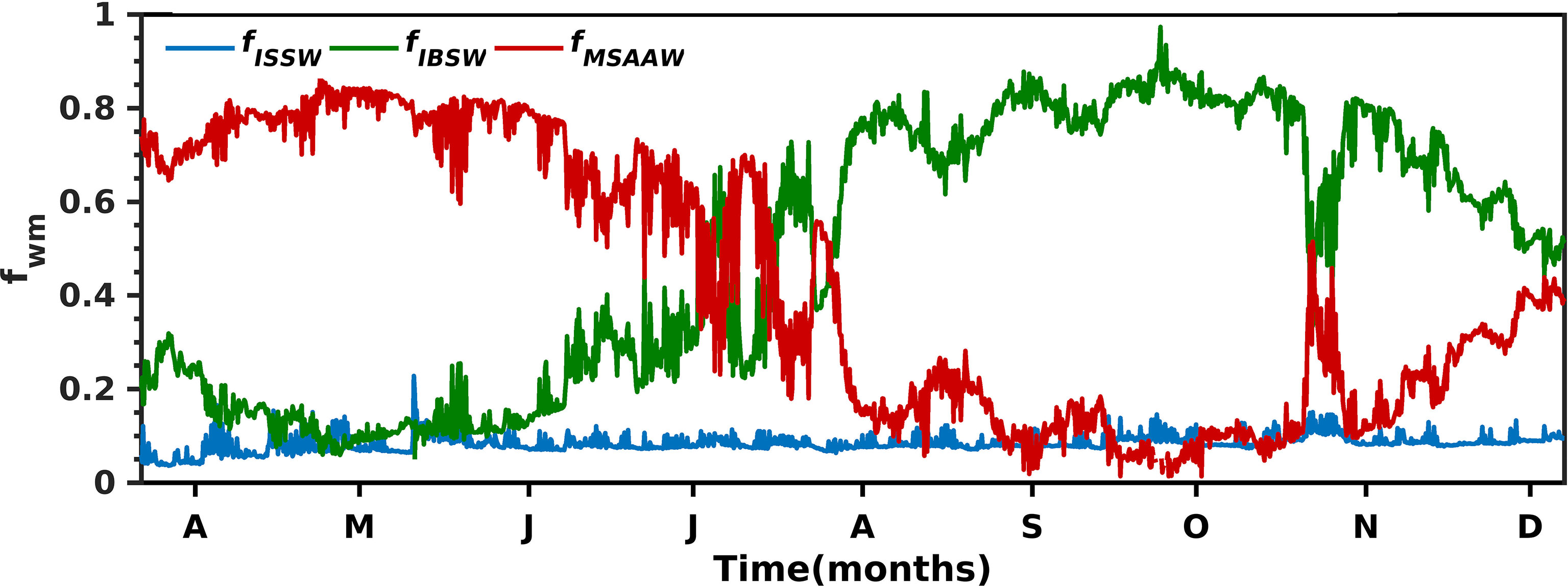
Figure 8 The seasonal variability of ISSW (Inner Surface Source Water), IBSW (Inner Bottom Source Water), MSAAW (Modified Subantarctic Water) in the upper 10 ± 1 m of the water column in the Seno Ballena Fjord mooring.

The carbonate system showed clear seasonality in the upper 10 m layer, with the most noticeable changes during fall and spring (Figure 7D). During fall, pCO₂ values had a mean of 385 ± 26 μatm (range 240 – 431 μatm). pCO₂ values decreased in spring, with a mean of 365 ± 47 μatm (range 167 – 471 μatm) and were associated with an increase in dissolved oxygen (negative values of AOU) and a decrease in salinity (Figure 7B). An increase of pCO₂ was observed in winter, which reached a mean of 394 ± 10 μatm (range 365 – 433 μatm), coincident with a decrease in temperature as the system changed from warming to cooling. A negative relationship was observed between pCO₂ normalized to an average temperature (npCO₂) and oxygen saturation percentage (%DO) (R² = 0.47, p<0.001; slope -3.7 μatm %DO^-1; Figure 9A). Although the npCO₂–salinity relationship had high scatter (Figure 9B), it showed a significant positive relationship during spring (R² = 0.30, p<0.001). The pCO₂–temperature relationship (Figure 9C) also showed a significant positive relationship during winter (R² = 0.41, p<0.001; Supplementary Table 2).

FIGURE 9

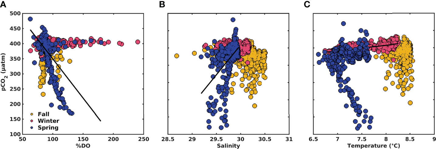
Figure 9 Relationships between (A) surface npCO₂-%DO, (B) npCO₂-Salinity, and pCO₂-Temperature (C) of time-series data. The yellow, pink and blue markers correspond to fall, winter, and spring, respectively. Black lines correspond to significant relationships of npCO₂-%OD during spring (R² = 0.47; p < 0.0001), npCO₂-Salinity during spring (R² = 0.30; p < 0.0001), and pCO₂-Temperature during winter (R² = 0.41; p < 0.0001).

Air-sea CO₂ fluxes varied from -3.08 mmol m^-2 d^-1 in spring to 0.29 mmol m^-2 d^-1 in winter (Figure 10A). CO₂ uptake in fall (March-May) fluctuated from -1.62 to -0.24 mmol m^-2 d^-1, while in spring (September to December) it varied from -0.57 to -3.08 mmol m^-2 d^-1. Degassing occurred only during the June-July winter months, with mean monthly fluxes of 0.09 and 0.26 mmol m^-2 d^-1, respectively. The data show continuous CO₂ absorption over seasons, indicating that this fjord behaves as a net sink of atmospheric CO₂ (mean = -1.01 mmol m^-2 d^-1). Water mass changes also played an important role in the change of DIC (range 41.39 - 180 μmol kg^-1) and therefore in pCO₂ (153 - 454 μatm). We observed large changes during the spring related to an influx of IBSW. The differences in DIC and pCO₂ at the mooring compared to a mixture of the water masses give the impact of the other factors: biology, air-sea gas exchange, and temperature (Figures 10A–C). The difference in DIC is always negative, which suggests that the mooring water mass always has more of a production signal, compared to a remineralization signal, than the underlying water types. These water masses are mainly subsurface water masses (ISBW and MSAAW) and have larger nutrient concentrations favoring primary productivity compared to the small contribution from the surface water mass (ISSW; Figure 8). The variability of pH_T was inversely correlated with pCO₂, showing maximum pH values during spring with a mean of 8.1 (range 8.0–8.3) and low values during winter and fall with a mean of 8.0 (range 8.0–8.1) (Figure 7E). The seasonal trend of pCO₂ and pH is followed by Ω_Ar (Figures 7D–F).

FIGURE 10

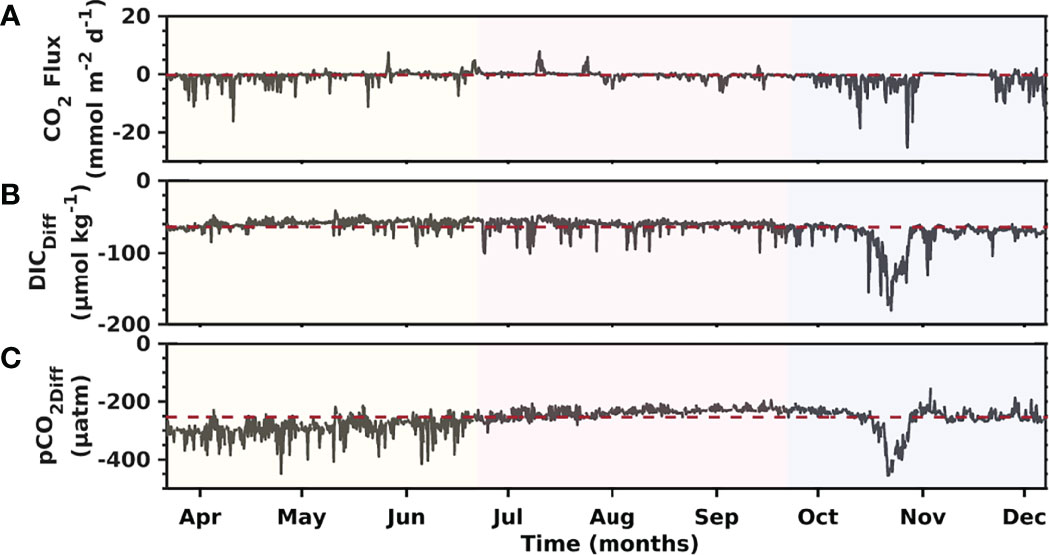
Figure 10 CO₂ flux (A), the difference between DIC_mooring and DIC_mix; the red dashed line is DIC_Diff mean (B), and the difference between pCO_2mooring and pCO_2mix; the red dashed line is pCO_2Diff mean (C) recorded from March to December, 2018 at the Seno Ballena Fjord.

4 Discussion

4.1 Hydrography and Nutrients

The results of our studies reveal the hydrographic control on the seasonal variability of the carbonate system, including the variability of the saturation state of seawater relative to calcium carbonate, pCO_2, and air-sea CO₂ fluxes (Figures 7, 10). Within the marine fjord system of Patagonia, we find fjords that are: (1) simple, two-layer vertical structures, with an estuarine surface layer of low salinity and a subsurface layer of oceanic origin with higher salinity (Schneider et al., 2014; Saldías et al., 2019); and (2) more complex three-layer structures as found in the Seno Reloncaví Fjord (Valle-Levinson et al., 2007). The above is modulated by freshwater contributions of glacial origin, river discharge, and rainfall, which significantly influence the salinity gradient of the surface layer in the vast coastal ocean of western Patagonia (Acha et al., 2004; Saldías et al., 2019).

Our results indicate that the Seno Ballena Fjord has two layers; the salinity of the surface layer is modulated by the input of meltwater from the glacier, mainly through stratifying the inner sill region of the fjord. The freshwater stratification and surface water salinity varied seasonally, with a relatively deeper halocline in fall and spring due to higher freshwater input (Figures 3, 4). The conditions were generally less stratified in winter, suggesting a limited supply of freshwater and strong ocean water contribution (Figure 3). As was observed in the water mass distribution analysis and the salinity gradients along the Seno Ballena Fjord, the influence of freshwater was higher on the inner-sill surface and reduced toward the outer-sill section. Only in spring does the freshwater plume spread past the sill (Figure 3), as has been observed in previous studies in this fjord during spring (Torres et al., 2011a). The observed seasonal variability of temperature and salinity was weaker (range Temp: 7.2 – 8.3°C/range S_P: 29.8 – 30.2) compared to other fjord systems of northern Patagonia (Seno Reloncaví (41°S); range Temp: 10.6 – 16.9°C/range S_P: 20.1 – 29.8) (Vergara-Jara et al., 2019) and western Canada (Strait of Georgia (49°N); S_P range: 5 – 29) (Moore-Maley et al., 2018), where strong seasonality in salinity is related to larger, seasonal river freshwater inputs (Puelo River: 713 to 4000 m³ s⁻¹ and Fraser River: 800 to 12.000 m³ s⁻¹).

The deep layer with higher salinity was influenced by the inflow of MSAAW: S_P = 31–33, which is modified upon entry into the Strait of Magellan, mixing with freshwater from rivers and melting glaciers, forming estuarine water with salinity around 28 – 31 S_P (Sievers and Silva, 2008). During tidal flood, the acceleration of the flow forces aspiration (Bernoulli aspiration; Valle-Levinson et al., 2007), pumping denser deep water which sinks below the less salty buoyant water in the inner section (Valle-Levinson et al., 2007). The high salinity-deeper water that flows inward compensates for the surface layer of freshwater that flows toward the Strait of Magellan. This type of circulation also influences the temperature of the fjord, causing an inverted thermocline with low surface temperature, underlain by a deep homogeneous layer of higher temperature. The low temperature in the surface layer of the Seno Ballena Fjord was more pronounced in winter due to the formation of a thin, surface layer of ice near the glacier, ice that likely is derived from re-frozen subglacial discharges rather than sea ice.

Our results in the Seno Ballena Fjord show that the nutrient concentrations were modulated inside and outside by the sill and revealed the significant spatial variability of nutrients (N and DSi), consistent with previous reports (Frangópulos et al., 2007). The presence of the shallow sill dividing the fjord causes a thin plume of low salinity water to spread over the sill during ebb tide (Torres et al., 2011a), which is probably modulated by the wind. The deepwater aspiration, when the water flow accelerates during the flood tide, probably influences the nutrient concentration patterns in the inner fjord (Figure 11; Valle-Levinson et al., 2006; Torres et al., 2011a). There is a strong influence of MSAAW, which has low DSi compared to nitrate concentrations, which explains the higher nitrate concentration in the deep water. In contrast, the continental waters of western Patagonia are characterized by high DSi and low nitrate, which explains the higher concentration of DSi in surface waters and near the glacier (Hervé et al., 2007; Torres et al., 2020). Plumes, tides and wind stress have also been found to drive circulation and renewal of the water masses of Northern Hemisphere fjords with sills, demonstrating their importance in the physical, chemical, and biological processes that occur inside and outside the fjords (Mortensen et al., 2011).

FIGURE 11

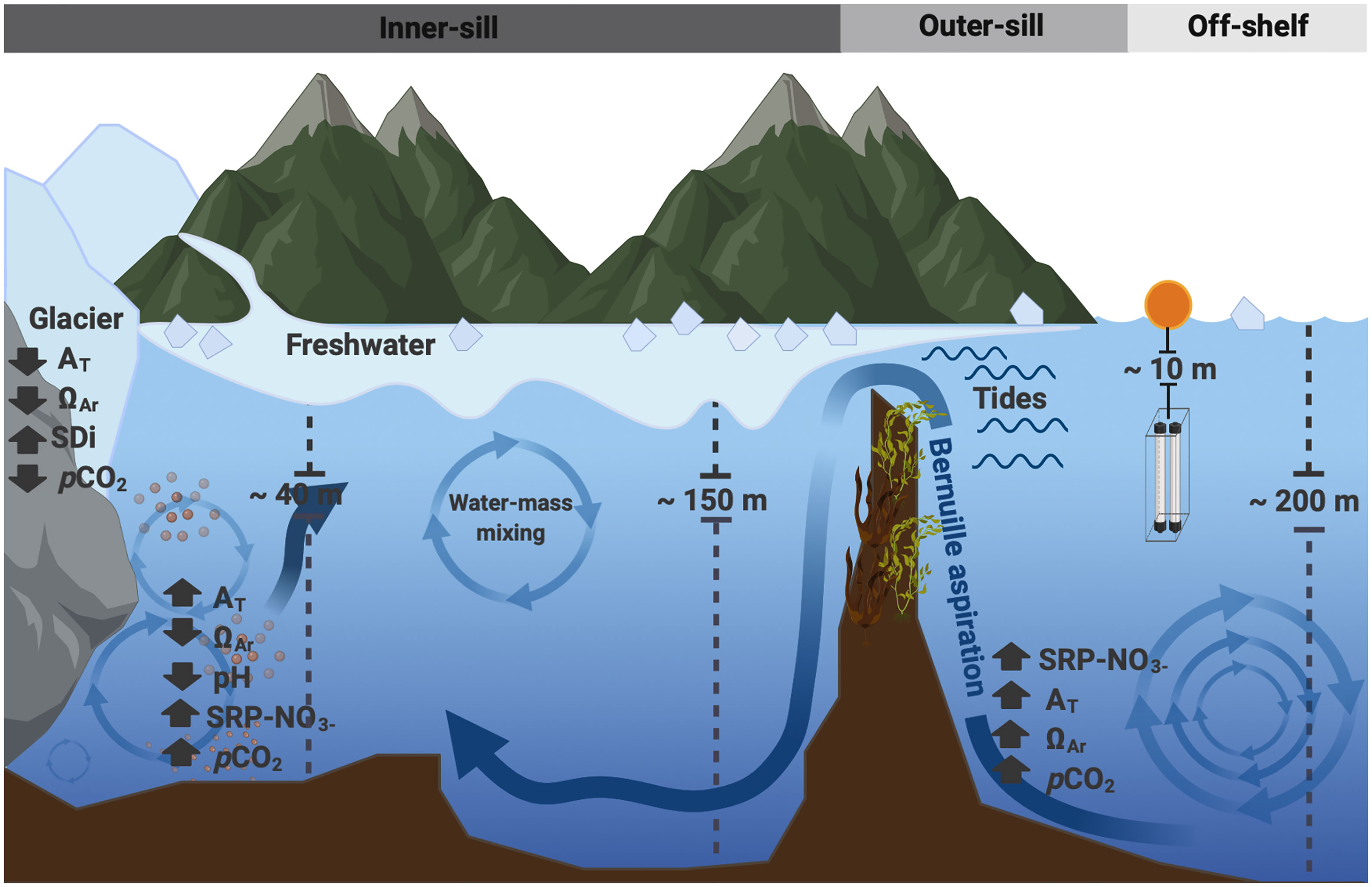
Figure 11 Schematic of processes that occur inside and outside of the Seno Ballena glacial fjord: (1) The input of freshwater from the marine-terminating glacier and river glacier may change physical-chemical properties, such as the following: i) generate strong surface stratification in the inner fjord section, ii) bring low A_T, low Ω_AR, low nutrients (SPR and NO₃), and low pCO₂, and iii) bring sediment and dissolved organic carbon (DOC). (2) Advection of subsurface nutrient-rich waters near the glacier. (3) Bernoulli aspiration caused by the fast shallow flow into the inner fjord is capable of sucking deep water coming from the Strait of Magellan up and over the sill. The density of this water mass then causes it to sink.

The plume of low salinity is blocked to a greater extent by the sill, particularly during low tide (Valle-Levinson et al., 2006). This blockage was observed during fall and spring. Hence, we suggest that the inner fjord residence time seems to allow the accumulation of local remineralization products such as nutrients and CO₂ in the inner fjord, allowing the IBSW to form near the glacier during fall and spring. IBSW represents the water mass observed near the glacier at subsurface levels (30 – 50 m), which has different properties (Figures 3, 5, 6) than those of the ISSW and MSAAW.

4.2 Carbonate Chemistry

The seasonal variability recorded in the Seno Ballena Fjord carbonate system can be assigned to several processes, including the input of freshwater from the melting of the Santa Inés glacier, the exchange with oceanic waters, biological production, seasonal variability in temperature, water column mixing and advection. The surface layer of the inner-sill region had undersaturated pCO₂ values with respect to the atmosphere during fall and spring, associated with the input of freshwater from the glacier (Figures 3, 4, 6). In this area, a higher fraction of ISSW is observed (range 1 to 0.3 of ISSB fraction, the surface to 10 m, respectively), which coincides with the lowest DIC_mix values (range 1489 - 1852 μmol kg^-1 of DIC_mix, surface to 10 m, respectively; Supplementary Figure 5), this indicates that the DIC input of freshwater was low and contributes to the decrease of the DIC of the mixture and directly to the pCO₂. These observations are consistent with previous studies in fjords and channels of Patagonia in which low-salinity surface waters (e.g. salinity less than 28) are strongly undersaturated in CO₂ (Torres et al., 2011b). Subglacial environments have low pCO₂ due to the effect of temperature (cooling), photosynthesis, and dilution (Bates and Mathis, 2009; Meire et al., 2015).

Although the pCO₂ was low in surface waters in the inner section of the fjord region during fall and spring, it did not result in the increase of calcium carbonate saturation (Ω_CaCO3: Ω_Ar and Ω_cal) whose variation seems to be dominated by dilution (i.e. the reduction of ${\text{CO}}_3^{-2}$ or Ca²⁺ ions by dilution with freshwater with very low levels of these ions). Our results were similar to conditions found in Alaska and Arctic fjords, where glacier fjords had low pCO₂ with respect to the atmosphere, and corrosive levels of aragonite (Ω_Ar) and calcite (Ω_cal) saturation near the surface (<50 m) due to the input of freshwater with low A_T and Ca²⁺ from glacier melting (Evans et al., 2014). The above finding suggests that the inner surface water of the Seno Ballena Fjord was under-saturated and corrosive to aragonite during the survey period, due to the intrusion of low A_T and Ca²⁺ (relationship Ω_Ar-A_T; R² = 0.42 n=50; p< 0.001) freshwater that drains the siliceous crystalline batholiths of Patagonia (Torres et al., 2011b; Torres et al., 2020). The above demonstrates the sensitivity of this Sub-Antarctic system to global stressors such as global warming and cooling, mainly for this Sub-Antarctic area where there has been a significant retreat of the glaciers in recent years (Bown et al., 2014).

The carbonate system presented clear seasonal variability in the outer sill region in March-December period, 2018 (Figure 7). A substantial reduction in pCO₂ and an increase in pH_T in spring months can be attributed to the dominance of photosynthesis (AOU: -191 μmol kg^-1) over respiration (%DO versus npCO₂, Figure 9; AOU Figure 7C). After the spring bloom, a signal of remineralization with higher values of pCO₂ (471 μatm) related to positive values of AOU (67 μmol kg^-1; Figure 7C) is observed, these results illustrate the key role that phytoplankton blooms and microbial respiration play in the variability of pCO₂, and therefore the change in pH and to a lesser extent the change in Ω_Ar, taking into account the signal that observed during the spring season that coincides in the three variables (pCO₂, pH_T, and Ω_Ar). In contrast, high pCO₂ values were recorded in winter, related to low pH_T and Ω_Ar, which could be attributed to subsurface water masses brought to the surface by increased water column mixing, which is more consistent between the months of July and August (IBSW and MSSAW; Figure 8) as well as the predominance of respiration over photosynthesis.

The variations recorded in the pCO₂ time-series seem to be driven by net primary productivity events due to the consistency of pCO₂ and dissolved oxygen variability (Figure 7). However, it should be borne in mind that the dynamics of coastal systems are also driven by other processes such as the mixing of different water masses; air-sea fluxes of CO_2, and variations in temperature. Therefore, in this study, these effects were also calculated (ΔpCO_2mix, ΔpCO_2gas, and ΔpCO_2tem, respectively). During spring, the biological processes (-4.72 to - 20.40 μatm day^-1), the changes in water mass (-5.42 to -17.2 μatm day^-1), and the sea-air CO₂ flux (-5.47 to - 21.81 μatm day^-1) contributed significantly to the decrease of pCO_2. The temperature effect is much smaller (-0.10 to 0.29 μatm day^-1). Similarly in fall, ΔpCO_2bio (22.68 to 30.13 μatm day^-1), ΔpCO_2mix (10.8 to 30.13 μatm day^-1), ΔpCO_2gas (11.25 to 30.72 μatm day^-1) dominate, which is why there are higher values of pCO₂ in fall compared to spring. The ΔpCO_2tem contribution is again small (Supplementary Table 4), as is observed in the linear regression of pCO₂/T (Figure 9). In contrast, in other studies, T is the most important factor in the variability of pCO₂, whereas in our studies it is the factor with the least importance in modulating the daily variability of pCO₂ (Xue et al., 2016).

The sea-air CO₂ flux varies seasonally, while low temperature and low haline stratification favors the positive sea-air CO₂ flux estimated in winter, the low wind speed limits those fluxes. In contrast, stronger winds during fall and spring contribute to the greater CO₂ uptake of Patagonian fjords. The mean wind speed was 4.04 m s^-1 during the study period, with a maximum monthly average of 6.04 m s^-1 (November) and a minimum of 3.73 m s^-1 (July; see Supplementary Figure 6). The higher CO₂ uptake in spring is also related to the decrease of pCO₂ in surface water by photosynthesis. Previous studies have also suggested that the fjords of Patagonia in warm seasons behave as a sink for CO₂ in response to high productivity (Torres et al., 2011b; Vergara-Jara et al., 2019). This behavior is also observed in fjords of the Northern Hemisphere (Meire et al., 2015).

Variation in pCO₂ is also driven by water mass changes. In fall, MASSW dominates with high values of DIC, whereas in spring, ISBW dominates with much lower DIC values. When these subsurface water masses are mixed to the surface, they bring macronutrients, products of remineralization, to the surface layer and favor primary productivity (Jones et al., 2020). The nutrient ratios (Si:N<1 and N:P<15) may indicate that the availability of silicic acid and nitrate plays a critical role in determining the extent and/or the persistence of phytoplankton blooms and the effects on the variability of the carbonate chemistry of waters in the study area, mainly in the spring season.

5 Conclusion

Frequent pCO₂ and pH_T measurements allowed us to determine that the carbonate system’s seasonal variability in the Seno Ballena Fjord was weaker compared to the northern Patagonia fjords. The most notable changes in pCO₂, pH_T, and Ω_Ar were driven by spring primary productivity, likely induced by the effect of seasonal increase of solar insolation in a recently stratified layer and local nutrient fertilization processes by the subsurface water mass ISBW (through aspiration and entrainment). In our results, we also found that the changes of the water masses play an important role in the daily variability of pCO₂ throughout the time series. In fall, MSAAW dominates with greater DIC contributing to the mixture and higher values of pCO₂ are recorded, whereas in spring the IBSW dominates with lower DIC compared to MSAAW, and lower pCO₂ values are recorded. The important role of mixing of the water masses ISSW, ISBW, and MSAAW and the air-sea exchange of CO₂ in the daily variability of pCO₂ was shown, which was generally just as important as biological processes. The very low freshwater-A_T end member means that meltwater significantly dilutes the concentration of A_T/DIC and calcium ions and plays a dominant role in driving low Ω_Ar values in estuarine waters (Figure 11). This study points out the importance of subglacial discharge from Santa Inés glacier in influencing the hydrography, nutrient, and carbonates system dynamics of the Seno Ballena Fjord, illustrating the sensitivity of this Sub-Antarctic system to global stressors such as global warming and freshening. The results highlight the important role of this high-latitude fjord as a CO₂ sink and the main processes driving this trend, including wind speed, low temperatures, and low salinity, these last two driven by surface freshwater runoff. These results suggest the importance of sustained high-resolution and long-term measurements of different physical and biogeochemical variables to understand the complex dynamics of the subantarctic fjords.

Data Availability Statement

The data of the sensor SAMI-CO₂, SAMI-pH, SBE37, and Aanderaa 5331A used for this study are publicly available and can be accessed at https://figshare.com/articles/dataset/Buoy_Seno_Ballena/12888008.

Author Contributions

JV was responsible for data processing and analysis, designed the manuscript, and wrote the manuscript. GS and SA. Participated in discussions on the data, review, and editing of the manuscript. MV-J Planning of the fieldwork methodology, installation, maintenance, and extraction of sensors data. MS and MD. Participated in part in the data analysis and review of the manuscript. RT. Participated in part in the data analysis. JI Participated in discussions on the data, review, editing, supervision of the manuscript, and funding acquisition. All authors approved the submitted version.

Funding

This project was supported by ANID-FONDECYT 1170174 (to J. L. Iriarte) and is part of the framework of Research Program 1 of the IDEAL Center (ANID-FONDAP 15150003).

Conflict of Interest

The authors declare that the research was conducted in the absence of any commercial or financial relationships that could be construed as a potential conflict of interest.

Publisher’s Note

All claims expressed in this article are solely those of the authors and do not necessarily represent those of their affiliated organizations, or those of the publisher, the editors and the reviewers. Any product that may be evaluated in this article, or claim that may be made by its manufacturer, is not guaranteed or endorsed by the publisher.

Acknowledgments

J.P Vellojin wishes to thank the School of Graduate Direction and the PhD program in Aquaculture Sciences at Universidad Austral de Chile, Campus Puerto Montt, and IDEAL Center for financial support during the 2017–2020 periods. Special thanks to Emerging Leaders of Americas (ELAP) Scholarships 2019 funded by Global Affairs Canada (GAC), managed by the Canadian Bureau for International Education (CBIE), for providing financial support to J.P Vellojin during the exchange program in the Department of Earth, Ocean and Atmospheric Sciences at the University of British Columbia, Canada. GSS thanks the partial funding from FONDECYT 1190805 and the Nucleus Center for the Study of Multiple-drivers on Marine Socio-Ecological Systems (MUSELS) funded by MINECON NC120086. Support at UBC was provided through NSERC Discovery Grant RGPIN-2016-03865 to SEA and Banting Post-doctoral Fellowship to GSS. MS was partially supported by INCAR (FONDAP-CONICYT No. 15110027). MD is supported by the U.S. National Science Foundation grant OPP-1723308. Special thanks to Marco Pinto for collaboration during the cruises carried out to Seno Ballena Fjord and Valeska Vasquez and Emilio Alarcón for collaboration in the sample analyses. The data presented are part of the Ph.D. thesis of Jurleys P. Vellojin at UACh. We thank the journal reviewers who made valuable suggestions and comments for improving the final version of the manuscript.

Supplementary Material

The Supplementary Material for this article can be found online at: https://www.frontiersin.org/articles/10.3389/fmars.2022.643811/full#supplementary-material

References

Acha E. M., Mianzan H. W., Guerrero R. A., Favero M., Bava J. (2004). Marine Fronts at the Continental Shelves of Austral South America: Physical and Ecological Processes. J. Mar. Syst. 44, 83–105. doi: 10.1016/j.jmarsys.2003.09.005

CrossRef Full Text | Google Scholar

Alarcón E., Valdés N., Torres R. (2015). Calcium Carbonate Saturation State in an Area of Mussels Culture in the Reloncaví Sound, Northern Patagonia, Chile. Lat. Am. J. Aquat. Res. 43, 277–281. doi: 10.3856/vol43-issue2-fulltext-1

CrossRef Full Text | Google Scholar

Bates N. R., Mathis J. T. (2009). The Arctic Ocean Marine Carbon Cycle: Evaluation of Air-Sea CO₂ Exchanges, Ocean Acidification Impacts and Potential Feedbacks. Biogeosciences 6, 2433–2459. doi: 10.5194/bg-6-2433-2009

CrossRef Full Text | Google Scholar

Bown F., Rivera A., Zenteno P., Bravo C., Cawkwell F., Raup (2014). “First Glacier Inventory and Recent Glacier Variation on Isla Grande De Tierra Del Fuego and Adjacent Islands in Southern Chile,” in Global Land Ice Measurements From Space Springer Praxis Books. Eds. Kargel J. S., Leonard G. J., Bishop M. P., Kääb A., Raup B. H. (Berlin, Heidelberg: Springer), 661–674. doi: 10.1007/978-3-540-79818-7_28

CrossRef Full Text | Google Scholar

Byrne R. H., Robert-Baldo G., Thompson S. W., Chen C. T. A. (1988). Seawater pH Measurements: An at-Sea Comparison of Spectrophotometric and Potentiometric Methods. Deep Sea Res. 35, 1405–1410. doi: 10.1016/0198-0149(88)90091-X

CrossRef Full Text | Google Scholar

Chierici M., Fransson A. (2009). Calcium Carbonate Saturation in the Surface Water of the Arctic Ocean: Undersaturation in Freshwater Influenced Shelves. Biogeosciences. 6, 2421–2431. doi: 10.5194/bg-6-2421-2009

CrossRef Full Text | Google Scholar

Chierici M., Fransson A., Lansard B., Miller L. A., Mucci A., Shadwick E., et al. (2011). Impact of Biogeochemical Processes and Environmental Factors on the Calcium Carbonate Saturation State in the Circumpolar Flaw Lead in the Amundsen Gulf, Arctic Ocean. J. Geophys. Res. Oceans 116, C00G09. doi: 10.1029/2011JC007184

CrossRef Full Text | Google Scholar

Chierici M., Fransson A., Nojiri Y. (2006). Biogeochemical Processes as Drivers of Surface fCO₂ in Contrasting Provinces in the Subarctic North Pacific Ocean. Glob. Biogeochem. Cycles 20, BG1009. doi: 10.1029/2004GB002356

CrossRef Full Text | Google Scholar

Clayton T. D., Byrne R. H. (1993). Spectrophotometric Seawater pH Measurements: Total Hydrogen Ion Concentration Scale Calibration of M-Cresol Purple and at-Sea Results. Deep Sea Res. 40, 2115–2129. doi: 10.1016/0967-0637(93)90048-8

CrossRef Full Text | Google Scholar

Cullison Gray S. E., DeGrandpre M. D., Moore T. S., Martz T. R., Friederich G. E., Johnson K. S. (2011). Applications of in Situ pH Measurements for Inorganic Carbon Calculations. Mar. Chem. 125, 82–90. doi: 10.1016/j.marchem.2011.02.005

CrossRef Full Text | Google Scholar

DeGrandpre M. D., Hammar T. R., Smith S. P., Sayles F. L. (1995). In Situ Measurements of Seawater pCO₂. Limnol. Oceanogr. 40, 969–975. doi: 10.4319/lo.1995.40.5.0969

CrossRef Full Text | Google Scholar

Dickson A. G. (1990). Standard Potential of the Reaction: AgCl(s) + 12H₂(G) = Ag(s) + HCl(aq), and the Standard Acidity Constant of the Ion HSO₄^– in Synthetic Sea Water From 273.15 to 318.15 K. J. Chem. Thermodyn. 22, 113–127. doi: 10.1016/0021-9614(90)90074-Z

CrossRef Full Text | Google Scholar

Dickson A. G., Goyet C. (1994). Handbook of Methods for the Analysis of the Various Parameters of the Carbon Dioxide System in Sea Water; Version 2 (Tennessee, United States: ORNL/CDIAC-74), 187.

Google Scholar

Dickson A. G., Millero F. J. (1987). A Comparison of the Equilibrium Constants for the Dissociation of Carbonic Acid in Seawater Media. Deep Sea Res. Part Oceanogr. Res. Pap. 34, 1733–1743. doi: 10.1016/0198-0149(87)90021-5

CrossRef Full Text | Google Scholar

Dickson A. G., Sabine C. L., Christian J. R. (2007). Guide to Best Practices for Ocean CO₂ Measurements Vol. 3 (Sidney, BC V8L 4B2 Canada: PICES Special Publication), 191.

Google Scholar

Ericson Y., Falck E., Chierici M., Fransson A., Kristiansen S., Platt S. M., et al. (2018). Temporal Variability in Surface Water Pco₂ in Adventfjorden (West Spitsbergen) With Emphasis on Physical and Biogeochemical Drivers. J. Geophys. Res. Ocean. 123, 4888–4905. doi: 10.1029/2018JC014073

CrossRef Full Text | Google Scholar

Evans W., Mathis J. T., Cross J. N. (2014). Calcium Carbonate Corrosivity in an Alaskan Inland Sea. Biogeosciences 11, 365–379. doi: 10.5194/bg-11-365-2014

CrossRef Full Text | Google Scholar

Feely R. A., Okazaki R. R., Cai W.-J., Bednaršek N., Alin S. R., Byrne R. H., et al. (2018). The Combined Effects of Acidification and Hypoxia on pH and Aragonite Saturation in the Coastal Waters of the California Current Ecosystem and the Northern Gulf of Mexico. Cont. Shelf. Res. 152, 50–60. doi: 10.1016/j.csr.2017.11.002

CrossRef Full Text | Google Scholar

Forcén-Vázquez A., Williams M. J. M., Bowen M., Carter L., Bostock H. (2021). Frontal Dynamics and Water Mass Variability on the Campbell Plateau. N. Z. J. Mar. Freshw. Res. 55, 199–222. doi: 10.1080/00288330.2021.1875490

CrossRef Full Text | Google Scholar

Forstner H., Gnaiger E. (1983). “Calculation of Equilibrium Oxygen Concentration,” in Polarographic Oxygen Sensors. Eds. Gnaiger E., Forstner H. (Berlin, Heidelberg: Springer), 321–333. doi: 10.1007/978-3-642-81863-9_28

CrossRef Full Text | Google Scholar

Frangópulos M., Blanco J., Hamamé M., Rosales S., Torres R., Valle-Levinson A. (2007) Análisis Y Diagnóstico De Las Principales Características Oceanográficas Del Área Marina Costera Protegida Francisco Coloane, Informe Proyecto Final GEF-PNUD “Conservación De La Biodiversidad De Importancia Mundial Al Largo De La Costa Chilena. Available at: http://cpps.dyndns.info/cpps-docs-web/planaccion/biblioteca/pordinario/102.articles-47869_InformeFinal.pdf (Accessed May 15, 2021).

Google Scholar

Fransson A., Chierici M., Hop H., Findlay H. S., Kristiansen S., Wold A. (2016). Late Winter-to-Summer Change in Ocean Acidification State in Kongsfjorden, With Implications for Calcifying Organisms. Polar. Biol. 39, 1841–1857. doi: 10.1007/s00300-016-1955-5

CrossRef Full Text | Google Scholar

Fransson A., Chierici M., Miller L. A., Carnat G., Shadwick E., Thomas H., et al. (2013). Impact of Sea-Ice Processes on the Carbonate System and Ocean Acidification at the Ice-Water Interface of the Amundsen Gulf, Arctic Ocean. J. Geophys. Res. Ocean. 118, 7001–7023. doi: 10.1002/2013JC009164

CrossRef Full Text | Google Scholar

Fransson A., Chierici M., Skjelvan I., Olsen A., Assmy P., Peterson A. K., et al. (2017). Effects of Sea-Ice and Biogeochemical Processes and Storms on Under-Ice Water fCO₂ During the Winter-Spring Transition in the High Arctic Ocean: Implications for Sea-Air CO₂ Fluxes. J. Geophys. Res. Ocean. 122, 5566–5587. doi: 10.1002/2016JC012478

CrossRef Full Text | Google Scholar

Fransson A., Chierici M., Yager P. L., Smith W. O. (2011). Antarctic Sea Ice Carbon Dioxide System and Controls. J. Geophys. Res. Oceans. 116, C12035. doi: 10.1029/2010JC006844

CrossRef Full Text | Google Scholar

Gac J.-P., Marrec P., Cariou T., Grosstefan E., Macé É., Rimmelin-Maury P., et al. (2021). Decadal Dynamics of the CO₂ System and Associated Ocean Acidification in Coastal Ecosystems of the North East Atlantic Ocean. Front. Mar. Sci. 8, 759.

Google Scholar

Garreaud R. D. (2018). Record-Breaking Climate Anomalies Lead to Severe Drought and Environmental Disruption in Western Patagonia in 2016. Clim. Res. 74, 217–229. doi: 10.3354/cr01505

CrossRef Full Text | Google Scholar

Giesecke R., Höfer J., Vallejos T., González H. E. (2019). Death in Southern Patagonian Fjords: Copepod Community Structure and Mortality in Land- and Marine-Terminating Glacier-Fjord Systems. Prog. Oceanogr. 174, 162–172. doi: 10.1016/j.pocean.2018.10.011

CrossRef Full Text | Google Scholar

Gran G. (1952). Determination of the Equivalence Point in Potentiometric Titrations. Part II. Analyst 77, 661–671. doi: 10.1039/AN9527700661

CrossRef Full Text | Google Scholar

Grear J. S., Rynearson T. A., Montalbano A. L., Govenar B., Menden-Deuer S. (2017). pCO₂ Effects on Species Composition and Growth of an Estuarine Phytoplankton Community. Estuar. Coast. Shelf. Sci. 190, 40–49. doi: 10.1016/j.ecss.2017.03.016

PubMed Abstract | CrossRef Full Text | Google Scholar

Haraldsson C., Anderson L. G., Hassellöv M., Hulth S., Olsson K. (1997). Rapid, High-Precision Potentiometric Titration of Alkalinity in Ocean and Sediment Pore Waters. Deep Sea Res. 44, 2031–2044. doi: 10.1016/S0967-0637(97)00088-5

CrossRef Full Text | Google Scholar

Hervé F., Pankhurst R. J., Fanning C. M., Calderón M., Yaxley G. M. (2007). The South Patagonian Batholith: 150 M Y of Granite Magmatism on a Plate Margin. Lithos. 97, 373–394. doi: 10.1016/j.lithos.2007.01.007

CrossRef Full Text | Google Scholar

Hopwood M. J., Carroll D., Dunse T., Hodson A., Holding J. M., Iriarte J. L., et al. (2020). Review Article: How Does Glacier Discharge Affect Marine Biogeochemistry and Primary Production in the Arctic? Cryosphere. 14, 1347–1383. doi: 10.5194/tc-14-1347-2020

CrossRef Full Text | Google Scholar

Ito T., Follows M. J., Boyle E. A. (2004). Is AOU a Good Measure of Respiration in the Oceans? Geophys. Res. Lett. 31, L17305. doi: 10.1029/2004GL020900

CrossRef Full Text | Google Scholar

Jackson J. M., Bianucci L., Hannah C. G., Carmack E. C., Barrette J. (2021). Deep Waters in British Columbia Mainland Fjords Show Rapid Warming and Deoxygenation From 1951 to 2020. Geophys. Res. Lett. 48, e2020GL091094. doi: 10.1029/2020GL091094

CrossRef Full Text | Google Scholar

Jones E. M., Renner A. H. H., Chierici M., Wiedmann I., Lødemel H. H., Biuw M. (2020). Seasonal Dynamics of Carbonate Chemistry, Nutrients and CO₂ Uptake in a Sub-Arctic Fjord. Elem. Sci. Anthr. 8, 41. doi: 10.1525/elementa.438

CrossRef Full Text | Google Scholar

Karstensen J. (2013) Análisis OMP (Optimum Multiparameter) - USER GROUP. Available at: https://omp.geomar.de/ (Accessed May 17, 2021).

Google Scholar

Karstensen J., Tomczak M. (1998). Age Determination of Mixed Water Masses Using CFC and Oxygen Data. J. Geophys. Res. Oceans. 103 (C9), 18599–18609. doi: 10.1029/98JC00889

CrossRef Full Text | Google Scholar

Kim H.-C., Lee K. (2009). Significant Contribution of Dissolved Organic Matter to Seawater Alkalinity. Geophys. Res. Lett. 36, L20603. doi: 10.1029/2009GL040271

CrossRef Full Text | Google Scholar

Kinder T. H., Bryden H. L. (1990). “Aspiration of Deep Waters Through Straits,” in The Physical Oceanography of Sea Straits NATO ASI Series. Ed. Pratt L. J. (Dordrecht: Springer Netherlands), 295–319. doi: 10.1007/978-94-009-0677-8_14

CrossRef Full Text | Google Scholar

Kurihara H. (2008). Effects of CO₂-Driven Ocean Acidification on the Early Developmental Stages of Invertebrates. Mar. Ecol. Prog. Ser. 373, 275–284. doi: 10.3354/meps07802

CrossRef Full Text | Google Scholar

Lafon A., Silva N., Vargas C. A. (2014). Contribution of Allochthonous Organic Carbon Across the Serrano River Basin and the Adjacent Fjord System in Southern Chilean Patagonia: Insights From the Combined Use of Stable Isotope and Fatty Acid Biomarkers. Prog. Oceanogr. 129, 98–113. doi: 10.1016/j.pocean.2014.03.004

CrossRef Full Text | Google Scholar

Li D., Chen J., Ni X., Wang K., Zeng D., Wang B., et al. (2018). Effects of Biological Production and Vertical Mixing on Sea Surface pCO₂ Variations in the Changjiang River Plume During Early Autumn: A Buoy-Based Time Series Study. J. Geophys. Res. Ocean. 123, 6156–6173. doi: 10.1029/2017JC013740

CrossRef Full Text | Google Scholar

Llanillo P. J., Pelegrí J. L., Duarte C. M., Emelianov M., Gasser M., Gourrion J., et al. (2012). Meridional and Zonal Changes in Water Properties Along the Continental Slope Off Central and Northern Chile. Cienc. Mar. 38, 307–332. doi: 10.7773/cm.v38i1B.1814

CrossRef Full Text | Google Scholar

Lukawska-Matuszewska K. (2016). Contribution of non-Carbonate Inorganic and Organic Alkalinity to Total Measured Alkalinity in Pore Waters in Marine Sediments (Gulf of Gdansk, S-E Baltic Sea). Mar. Chem. 186, 211–220. doi: 10.1016/j.marchem.2016.10.002

CrossRef Full Text | Google Scholar

Mamayev O. I. (1975). Temperature-Salinity Analysis of World Ocean Waters. 1st Edition (Canada: Elsevier Science).

Google Scholar

McDougall T. J., Barker P. M. (2011). Getting Started With TEOS-10 and the Gibbs Seawater (GSW) Oceanographic Toolbox. Scor/Iapso WG, 127, 1–28.

Google Scholar

Mehrbach C., Culberson C. H., Hawley J. E., Pytkowicx R. M. (1973). Measurement of the Apparent Dissociation Constants of Carbonic Acid in Seawater at Atmospheric Pressure1. Limnol. Oceanogr. 18, 897–907. doi: 10.4319/lo.1973.18.6.0897

CrossRef Full Text | Google Scholar

Meier W. J.-H., Grießinger J., Hochreuther P., Braun M. H. (2018). An Updated Multi-Temporal Glacier Inventory for the Patagonian Andes With Changes Between the Little Ice Age and 2016. Front. Earth Sci. 6. doi: 10.3389/feart.2018.00062

CrossRef Full Text | Google Scholar

Meire L., Søgaard D. H., Mortensen J., Meysman F. J. R., Soetaert K., Arendt K. E., et al. (2015). Glacial Meltwater and Primary Production are Drivers of Strong CO₂ Uptake in Fjord and Coastal Waters Adjacent to the Greenland Ice Sheet. Biogeosciences. 12, 2347–2363. doi: 10.5194/bg-12-2347-2015

CrossRef Full Text | Google Scholar

Meredith M., Sommerkorn M., Cassotta S., Derksen C., Ekaykin A., Hollowed A., et al. (2019). “Chapter 3: Polar Regions. In: Polar Regions,” in IPCC Special Report on the Ocean and Cryosphere in a Changing Climate. Eds. Pörtner H.-O., Roberts D. C., Masson-Delmotte V., Zhai P., Tignor M., Poloczanska E., Mintenbeck K., Alegría A., Nicolai M., Okem A., Petzold J., Rama B., Weyer N. M.(Ginebra), 203–320.

Google Scholar

Moore-Maley B. L., Ianson D., Allen S. E. (2018). The Sensitivity of Estuarine Aragonite Saturation State and pH to the Carbonate Chemistry of a Freshet-Dominated River. Biogeosciences. 15, 3743–3760. doi: 10.5194/bg-15-3743-2018

CrossRef Full Text | Google Scholar

Mortensen J., Lennert K., Bendtsen J., Rysgaard S. (2011). Heat Sources for Glacial Melt in a Sub-Arctic Fjord (Godthåbsfjord) in Contact With the Greenland Ice Sheet. J. Geophys. Res. Ocean. 116, C01013. doi: 10.1029/2010JC006528

CrossRef Full Text | Google Scholar

Orr J. C., Fabry V. J., Aumont O., Bopp L., Doney S. C., Feely R. A., et al. (2005). Anthropogenic Ocean Acidification Over the Twenty-First Centuryand its Impact on Calcifying Organisms. Nature. 437, 681–686. doi: 10.1038/nature04095

PubMed Abstract | CrossRef Full Text | Google Scholar

Parsons T. R., Maita Y., Lalli C. M. (1984). A Manual of Chemical& Biological Methods for Seawater Analysis (Ox ford, UK: Pergamon Press).

Google Scholar

Pierrot D., Lewis E., Wallace D. W. R. (2006). MS Excel Program Developed for CO2 System Calculations. ORNL/CDIAC-105 (Washington, D.C: U.S. Department of Energy).

Google Scholar

Pytkowicx R. M. (1971). On the Apparent Oxygen Utilization and the Preformed Phosphate in the Oceans1. Limnol. Oceanogr. 16, 39–42. doi: 10.4319/lo.1971.16.1.0039

CrossRef Full Text | Google Scholar

Saldías G. S., Sobarzo M., Quiñones R. (2019). Freshwater Structure and its Seasonal Variability Off Western Patagonia. Prog. Oceanogr. 174, 143–153. doi: 10.1016/j.pocean.2018.10.014

CrossRef Full Text | Google Scholar

Sarmiento J. L., Gruber N., Brzezinski M. A., Dunne J. P. (2004). High-Latitude Controls of Thermocline Nutrients and Low Latitude Biological Productivity. Nature. 427, 56–60. doi: 10.1038/nature02127

PubMed Abstract | CrossRef Full Text | Google Scholar

Schneider W., Pérez-Santos I., Ross L., Bravo L., Seguel R., Hernández F. (2014). On the Hydrography of Puyuhuapi Channel, Chilean Patagonia. Prog. Oceanogr. 129, 8–18. doi: 10.1016/j.pocean.2014.03.007

CrossRef Full Text | Google Scholar

Sievers H. A., Calvete C., Silva N. (2002). Distribución De Características Físicas, Masas De Agua Y Circulación General Para Algunos Canales Australes Entre El Golfo De Penas Y El Estrecho De Magallanes (Crucero CIMAR-2 Fiordos). Rev. Cienc. Tecnol. Mar. 25, 17–43.

Google Scholar

Sievers H. A., Silva N. (2008). “Water Masses and Circulation in Austral Chilean Channels,” in Progress in the Oceanographic Knowledge of Chilean Interior Waters, From Puerto Montt to Cape Horn. Eds. Silva N., Palma S. (Valparaíso, Chile: Comité Oceanográfico Nacional), 53–58.

Google Scholar

Silva N., Calvete C., Sievers H. (1998). Masas De Agua Y Circulación General Para Algunos Canales Australes Entre Puerto Montt Y Laguna San Rafael, Chile (Crucero Cimar-Fiordo 1). Cienc. Tecnol. Mar. 21, 17–48.

Google Scholar

Silva N., Rojas N., Fedele A. (2009). Water Masses in the Humboldt Current System: Properties, Distribution, and the Nitrate Deficit as a Chemical Water Mass Tracer for Equatorial Subsurface Water Off Chile. Deep. Sea. Res. Part II. Top. Stud. Oceanogr. 56, 1004–1020. doi: 10.1016/j.dsr2.2008.12.013

CrossRef Full Text | Google Scholar

Takahashi T., Sutherland S. C., Wanninkhof R., Sweeney C., Feely R. A., Chipman D. W., et al. (2009). Climatological Mean and Decadal Change in Surface Ocean Pco₂, and Net Sea–Air CO₂ Flux Over the Global Oceans. Deep. Sea. Res. Part II. Top. Stud. Oceanogr. 56, 554–577. doi: 10.1016/j.dsr2.2008.12.009

CrossRef Full Text | Google Scholar

Takahashi T., Olafsson J., Goddard J. G., Chipman D. W., Sutherland S. (1993). Seasonal Variation of CO₂ and Nutrients in the High-Latitude Surface Oceans: A Comparative Study. Glob. Biogeochem. Cycles 7 (4), 843–878.

Google Scholar

Torres R., Frangópulos M., Hamamé M., Montecino V., Maureira C., Pizarro G., et al. (2011a). Nitrate to Silicate Ratio Variability and the Composition of Micro-Phytoplankton Blooms in the Inner-Fjord of Seno Ballena (Strait of Magellan, 54°s). Cont. Shelf. Res. 31, 244–253. doi: 10.1016/j.csr.2010.07.014

CrossRef Full Text | Google Scholar

Torres R., Pantoja S., Harada N., González H. E., Daneri G., Frangopulos M., et al. (2011b). Air-Sea CO₂ Fluxes Along the Coast of Chile: From CO2 Outgassing in Central Northern Upwelling Waters to CO₂ Uptake in Southern Patagonian Fjords. J. Geophys. Res. Ocean. 116, C09006. doi: 10.1029/2010JC006344

CrossRef Full Text | Google Scholar

Torres R., Reid B., Frangópulos M., Alarcón E., Márquez M., Häussermann V., et al. (2020). Freshwater Runoff Effects on the Production of Biogenic Silicate and Chlorophyll-a in Western Patagonia Archipelago (50–51°s). Estuar. Coast. Shelf. Sci. 241, 106597. doi: 10.1016/j.ecss.2020.106597

CrossRef Full Text | Google Scholar

Torres R., Silva N., Reid B., Frangopulos M. (2014). Silicic Acid Enrichment of Subantarctic Surface Water From Continental Inputs Along the Patagonian Archipelago Interior Sea (41–56°s). Prog. Oceanogr. 129, 50–61. doi: 10.1016/j.pocean.2014.09.008

CrossRef Full Text | Google Scholar

UNESCO, I (1981). The Practical Salinity Scale 1978 and the International Equation of State of Seawater 1980. Tenth. Rep. Jt. Panel. Oceanogr. Table. Stand. JPOTS. 25, 36.

Google Scholar

Uppström L. R. (1974). The boron/chlorinity ratio of Deep-Sea Water From the Pacific Ocean. Deep-Sea Res 21, 161–162. doi: 10.1016/0011-7471(74)90074-6

CrossRef Full Text | Google Scholar

Valdenegro A., Silva N. (2003). Caracterización Oceanográfica Física Y Química De La Zona De Canales Y Fiordos Australes De Chile Entre El Estrecho De Magallanes Y Cabo De Hornos (Cimar 3 Fiordos). Cienc. Tecnol. Mar. 26, 16–60.

Google Scholar

Valle-Levinson A., Blanco J. L., Frangópulos M. (2006). Hydrography and Frontogenesis in a Glacial Fjord Off the Strait of Magellan. Ocean. Dyn. 56, 217–227. doi: 10.1007/s10236-005-0048-8

CrossRef Full Text | Google Scholar

Valle-Levinson A., Sarkar N., Sanay R., Soto D., León J. (2007). Spatial Structure of Hydrography and Flow in a Chilean Fjord, Estuario Reloncaví. Estuar. Coast. 30, 113–126. doi: 10.1007/BF02782972

CrossRef Full Text | Google Scholar

Vergara-Jara M. J., DeGrandpre M. D., Torres R., Beatty C. M., Cuevas L. A., Alarcón E., et al. (2019). Seasonal Changes in Carbonate Saturation State and Air-Sea CO₂ Fluxes During an Annual Cycle in a Stratified-Temperate Fjord (Reloncaví Fjord, Chilean Patagonia). J. Geophys. Res. Biogeosci. 124, 2851–2865. doi: 10.1029/2019JG005028

CrossRef Full Text | Google Scholar

Wanninkhof R. (1992). Relationship Between Wind Speed and Gas Exchange Over the Ocean. J. Geophys. Res. Ocean. 97, 7373–7382. doi: 10.1029/92JC00188

CrossRef Full Text | Google Scholar

Wanninkhof R. (2014). Relationship Between Wind Speed and Gas Exchange Over the Ocean Revisited. Limnol. Oceanogr. Methods 12, 351–362. doi: 10.4319/lom.2014.12.351

CrossRef Full Text | Google Scholar

Weiss R. F. (1974). Carbon Dioxide in Water and Seawater: The Solubility of a non-Ideal Gas. Mar. Chem. 2, 203–215. doi: 10.1016/0304-4203(74)90015-2

CrossRef Full Text | Google Scholar

Xue L., Cai W.-J., Hu X., Sabine C., Jones S., Sutton A. J., et al. (2016). Sea Surface Carbon Dioxide at the Georgia Time Series Site, (2006–2007): Air–sea Flux and Controlling Processes. Prog. Oceanogr. 140, 14–26. doi: 10.1016/j.pocean.2015.09.008

CrossRef Full Text | Google Scholar