Analysis of the accuracy of using ERA5 reanalysis data for diagnosis of evaporation ducts in the East China Sea

Evaporation ducts are a phenomenon that occurs with extremely high frequency at the boundary between the atmosphere and the ocean. Because they directly affect the propagation of electromagnetic waves, it is necessary to study their various characteristics. Since it is difficult to conduct large-scale observations at sea, many researchers use reanalysis data for this task instead of observation data. However, there have been no studies verifying accuracy of this analysis method for the diagnosis of evaporation ducts. Therefore, in this work, observations of the low-altitude atmospheric refractivity profile were carried out over the East China Sea on board the research vessel Xiangyanghong 18 in April 2021. First, the differences between different evaporation duct models were examined based on the meteorological and hydrological data obtained at different heights. It was concluded that the diagnostic accuracy of the evaporation duct model is low in stable conditions and a low-wind-speed environment. Under the same conditions, the Naval Postgraduate School (NPS) model showed high diagnostic accuracy when compared with other models. Second, Taylor plots were used to verify the accuracy of the reanalysis data and the observation data. It was concluded that the single-parameter precision of the reanalysis data is relatively high, and there were strong correlations with the observation data. Finally, the observation and reanalysis data were used to compare and analyze the false-report rate, the missing-report rate, and the accuracy of the diagnosed evaporation duct height using the NPS model. The false-report rate and missing-report rate were found to be 1.93% and 1.52%, respectively. The average diagnosis deviation was 3.34 m. The Pearson correlation coefficient was found to be close to 1. The results indicate that it is basically feasible to analyze the characteristics of evaporation ducts based on the NPS model using reanalysis data.

1. Introduction

Evaporation ducts occur because of atmospheric stratification formed by the rapid decrease of water vapor with height near the sea surface; they are typically generated by ocean–atmosphere interactions. Research has shown that the probability of an evaporation duct occurring in the South China Sea exceeds 80% (Yang et al., 2017; Qiu et al., 2022). Evaporation ducts can cause anomalous propagation of electromagnetic (EM) waves, especially in the microwave band (Hitney and Vieth, 1990; Lentini and Hackett, 2015). On the one hand, trapped EM waves can propagate with lower loss in the ducting layer, which can realize beyond-the-horizon detection. On the other hand, an evaporation duct will allow EM waves of frequencies higher than the lowest trapped frequency and incident angle less than the critical angle to enter the ducting layer, causing a radar blind zone at a certain angle. As shown in Figure 1, the evaporation duct parameters—height (EDH) and strength (EDS)—directly affect the transmission path of EM waves on the sea surface (Wang et al., 2018). Therefore, accurate diagnosis of evaporation duct parameters is of great significance to maritime radio communications and radar target detection (Zhang et al., 2016a; Zaidi et al., 2018; Shi et al., 2019;).

FIGURE 1

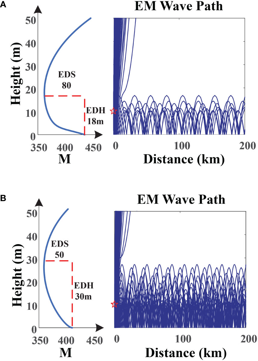
Figure 1 Differences in EM-wave transmission paths under different EDH and EDS values. (A) EDH = 18 m, EDS = 80; (B) EDH = 30 m, EDS = 50.

Refraction, the cause of the evaporation duct phenomenon, can be characterized by the vertical gradients in the atmospheric refractive index n. To more conveniently represent and account for the curvature of the Earth, n is usually replaced with a modified refractivity M, which is related to the atmospheric pressure AP (hPa), air temperature AT (K), partial pressure of water vapor e (hPa), and height above the sea surface z (m) through the equation:

$\begin{array}{ll}M=77.6\frac{AP}{AT}-5.6\frac{e}{AT}+3.73\frac{e}{A{T}^2}+0.157z& (1)\end{array}$

When using multiple meteorological observational data points from different heights to calculate the EDH, a least-squares fitting method is usually used to obtain the corresponding vertical profile of M (Babin et al., 1997). This profile is based on a log-linear function given by

$\begin{array}{ll}M=f_{0}z-f_1\ln (z+0.001)+f_2& (2)\end{array}$

The constant 0.001 is added to prevent ln(0) from occurring at the sea surface. For each case, the coefficients f₀ , f₁ , and f₂ can be calculated for a least-squares best fit. The EDH is defined as the height at which ∂M/∂z is equal to 0 , or, equivalently, the height at which M is a minimum (Almond and Clarke, 1983). As shown in Figure S1, the difference between the modified refractivity M at height 0 and the modified refractivity M at the EDH is the EDS.

Currently, the main methods for obtaining the evaporation duct parameters are:

a. Using a refractometer to directly measure the atmospheric refractivity at different heights (Chai et al., 2022);

b. Using a radiosonde and meteorological observation towers to measure meteorological parameters at different heights and indirectly calculating the vertical distribution of atmospheric refractivity (Liu et al., 1979; Karimian et al., 2012);

c. Using an evaporation duct model (EDM) based on meteorological and hydrological parameters (Sun et al., 2016; Zhang et al., 2017).

The basic principle of the last method is the Monin–Obukhov similarity theory. By measuring the wind speed (WS), air temperature (AT), relative humidity (RH), and air pressure (AP) at certain heights and the sea-surface temperature (SST), an empirical model can be developed to calculate the vertical distribution of atmospheric refractivity, and the evaporation duct parameters can then be obtained. Because of its convenient operation, this method has received extensive attention. Many EDMs have been proposed, including the Paulus–Jeske (Jeske, 1973), Babin–Young–Carton (BYC) (Babin et al., 1997), revised fifth-generation mesoscale (MM5REV) (Jiao and Zhang, 2015), Naval Postgraduate School (NPS) (Frederickson et al., 2000), Naval Warfare Assessment (NWA) (Liu and Blanc, 1984), Liu-Katsaros-Businger (LKB) (Babin and Dockery, 2002), and Coupled Ocean–Atmosphere Response Experiment (Fairall et al., 2003) models. These models all take atmospheric stratification into account. Atmospheric stratification is an important factor affecting an evaporation duct. In physical oceanography, the Richardson number (Ri) is usually used to characterize atmospheric stratification: Ri > 0 , = 0 , and < 0 respectively indicate that the atmosphere is in a stable, neutral, or unstable condition. In current boundary-layer parameterization schemes, Ri is usually set as a semi-empirical parameter, and different EDMs use different calculation methods for this. Although these EDMs are all based on the Monin-Obukhov similarity theory, they show different diagnostic results under different meteorological and hydrological environments. The uncertainty of the theoretical model is from the empirical parameters (the stability functions and roughness length parameterization) of the model, these parameters are derived from local observations. Which EDMs is more suitable for the East China Sea needs to be verified by actual ocean observation data.

To research the evolution rules and distribution characteristics of evaporation ducts, it is necessary to obtain real-time meteorological and hydrological data; however, this is very difficult at sea. Therefore, many researchers have started to use reanalysis data and apply EDMs to study the occurrence laws of evaporation ducts in particular areas. Since the 1980s, the US Navy has attempted to study atmospheric ducts using mesoscale weather models (Burk and Thompson, 1989). Since the mid-1990s, the US Naval Research Laboratory (NRL) has been developing a three-dimensional ocean–atmosphere coupled mesoscale forecast system (COAMPS). With continuous improvement of the data-assimilation system, wave parameterization, boundary-layer scheme, etc., this system has been deployed for many years in US Navy combat forecasts and applied to an evaporation duct numerical weather-prediction system (Hodur, 1997; Zhao et al., 2016). Zhu and Atkinson (2005) used the third-generation mesoscale (MM3) model to conduct one-year hindcasted predictors in the Persian Gulf and analyze the seasonal characteristics of evaporation ducts. Haack et al. (2010) used four mesoscale numerical weather-prediction models on the eastern coast of the United States to simulatethe atmospheric refractive index and duct-layer structure; they found that the characteristics of evaporation ducts are highly correlated with the SST , atmospheric stability, and underlying surface roughness.

The reanalysis data used in the above research assimilate a large amount of satellite and conventional observational data; this has the advantages of covering long time periods with high resolution. Since the 1990s, the United States, Europe, Japan, and other countries have successively developed reanalysis data products, including National Centers for Environmental Prediction/National Center for Atmospheric Research (NCEP/NCAR) (American reanalysis data; ARD), National Centers for Environmental Prediction-Department of Energy (NCEP/DOE) (ARD), NCEP Climate Forecast System Reanalysis (CFSR) (ARD), Climate Forecast System version 2 (CFSv2) (ARD), Japanese 25-year Reanalysis project (JRA) (Japanese reanalysis data; JRD), Japanese 55-year Reanalysis (JRA55) (JRD) (Zhang et al., 2016b). The European Center for Medium-Range Weather Forecasts (ECMWF) was one of the early institutions to reanalyze data, and it developed the First Global Atmospheric Research Program Global Experiment (FGGE), ECMWF Reanalysis-40 years (ERA-40), and ERA-Interim datasets. In 2016, the ECMWF released the fifth-generation reanalysis product ERA5. Many researchers have analyzed the accuracy of different elements of reanalysis data, and they have generally concluded that the ERA5 data has higher accuracy than other available products (Shi et al., 2021). In 2015, the China Meteorological Administration (CMA) developed the Land Data Assimilation System (CLDAS-CMA), which includes high-precision WS, AT, RH, and AP data in the seas near China, but it does not include SST. Research has shown that the accuracy of reanalysis data is highly correlated with the change trends of actual observation data (Luo et al., 2019). Tian et al. (2020) tried to analyze the influence of seasonal and nonreciprocal evaporation ducts on EM wave propagation in the Gulf of Aden by using ERA5 to reanalyze the data. However, due to the difficulty of obtaining ocean-observation data, the accuracy of this kind of analysis needs to be further verified (Meng et al., 2018).

In summary, the environmental suitability of different EDMs to the East China Sea and the feasibility of using reanalysis data to study evaporation duct characteristics need to be verified. However, the above research needs to rely on the actual offshore evaporation duct observation data. In view of the lack of observational data relating to evaporation ducts at sea, an observation of the low-altitude atmospheric refractivity profile was carried out over the East China Sea. This was conducted on board the research vessel (R/V) Xiangyanghong 18. To obtain the atmospheric refractive index at different heights, five layers of meteorological and hydrological sensors were installed on the hull at different heights in the range 6–25 m, and a 25-day low-altitude atmospheric refractive-index-profile observation was carried out. Observation data, including WS, AT, RH, AP, and SST, were obtained under different time and space conditions, and these were analyzed and compared. First, the accuracy of the atmospheric refractive indexes obtained under different meteorological and hydrological conditions at different heights using different EDMs was analyzed and studied; second, the CLDAS and ERA5 reanalysis data were compared with the actual observation data; finally, the evaporation duct parameters obtained from the observations and from the ERA5 reanalysis data were examined and compared. The false-alarm rate, missing-report rate, and accuracy of the diagnosis results obtained using the reanalysis data were calculated. This study provides experimental verification for the subsequent use of reanalysis data to analyze the characteristics of evaporation ducts.

2. Data

The data used in this paper include the ocean-observation, ERA5 and CLDAS datasets.

2.1. Ocean-observation dataset

From the National Natural Science Foundation of China Open Research Voyage (Voyage No. NORC2021-02+NORC2021-301), different temporal and spatial meteorological and hydrological gradient observations in the East China Sea (as shown in Figure 2) were obtained from the 00:00:00 UTC+8 8 April 2021 to 23:59:59 UTC+8 24 April 2021. To obtain meteorological and hydrological parameters at different altitudes, as shown in Figure 3, five layers of high-precision HUMICAP sensors were installed on the bow deck (6.0 m), accommodation deck (8.3 m), compass deck (13.1 m), first-layer mast (14.8 m), and third-layer mast (22.3 m) of the R/V Xiangyanghong 18 (IMO 9769506) to achieve layered measurements of AT and RH at different heights. An Airmar WeatherStation and a barometric pressure sensor were installed in the middle of the living deck to obtain observation data of WS and AP , respectively. A pair of infrared temperature sensors was installed on the port and starboard to obtain the SST . All observation data were sent to a data collector in the ship’s data center through communication cables. The collection frequency was set to 1 Hz.

FIGURE 2

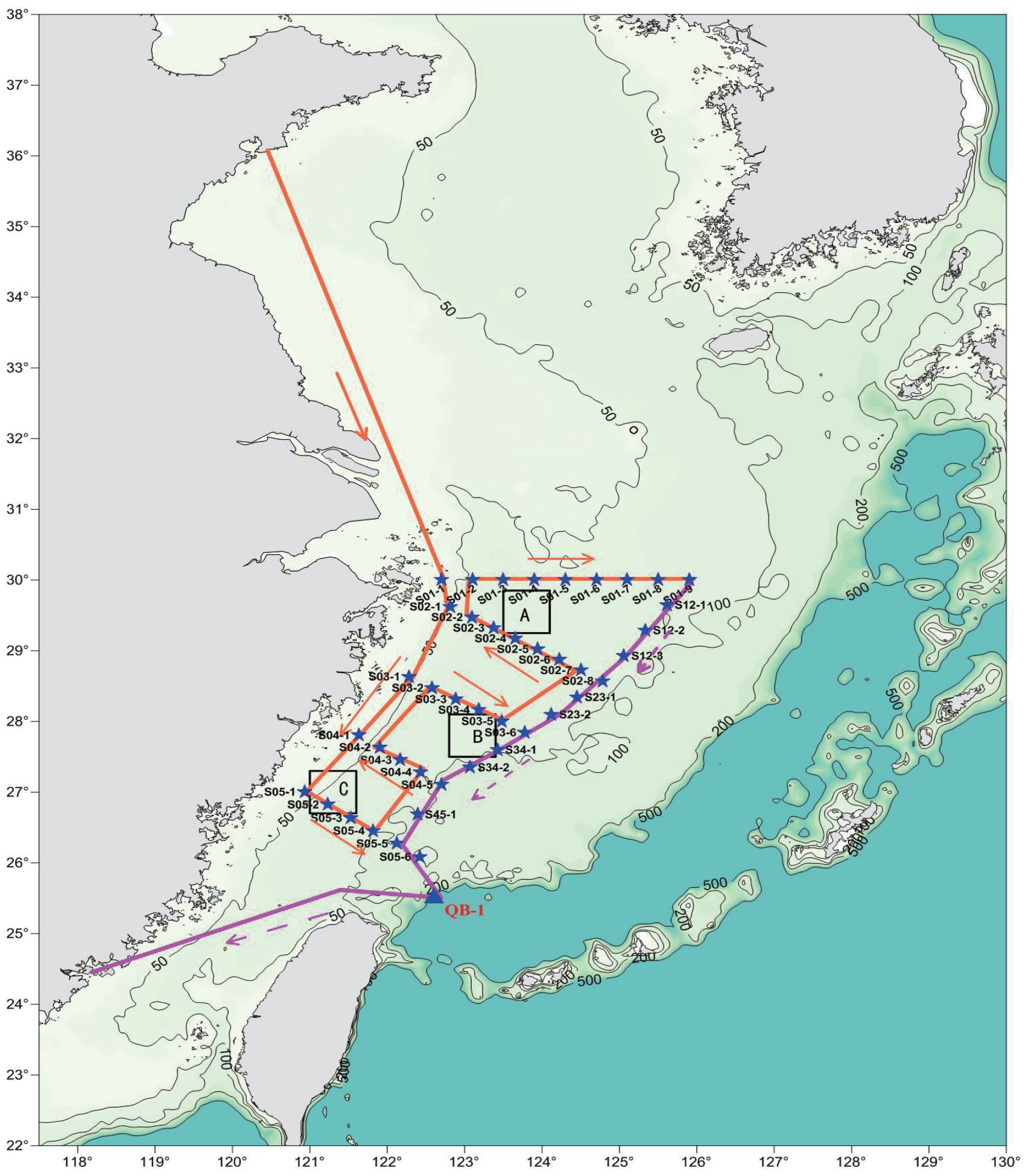
Figure 2 Station and route map of the voyage. Select three areas from north to south (areas A, B, and C in the figure), and the ship will sail back and forth in these areas.

FIGURE 3

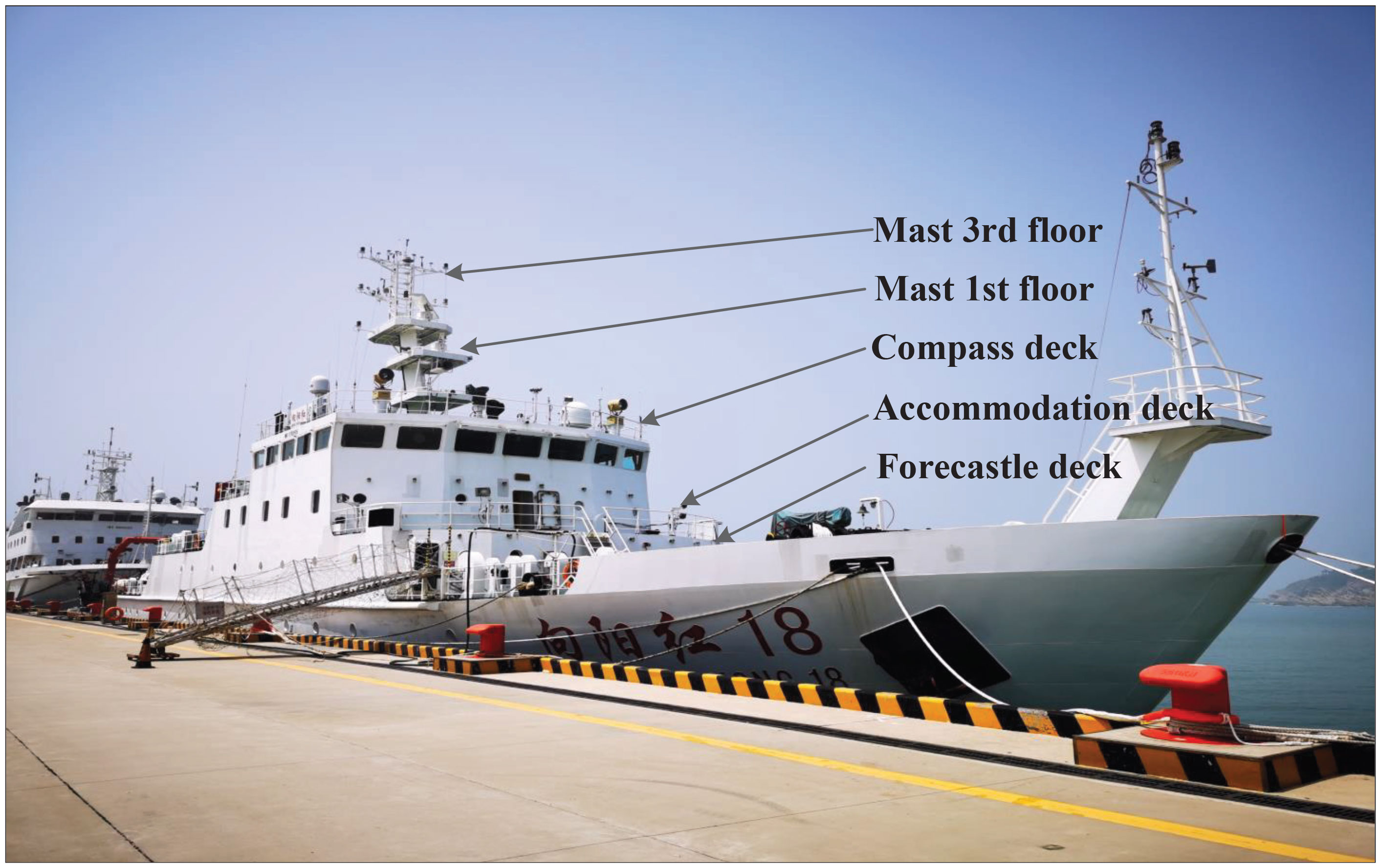
Figure 3 Schematic diagram of the sensor installation positions of the R/V Xiangyanghong 18 (IMO 9769506).

To ensure the accuracy of the observed data, high-precision sensors were used and appropriate sensor calibrations were performed. The sensor parameters and their installation locations are shown in Table 1.

TABLE 1

Table 1 Sensor parameters and installation location information.

2.2. ERA5 dataset

The ERA5 reanalysis data is the latest generation of reanalysis data to be created by the ECMWF. It was first released in January 2019. These data can be used for tasks such as climate monitoring and numerical weather forecasting. The ERA5 product has been further upgraded on the basis of the previous series of reanalysis data products released by the ECMWF. More historical observation data, especially satellite data, have been applied to the advanced data assimilation and model system to estimate atmospheric conditions more accurately. ERA5 provides more variables, including AT, AP, wind force at different heights, rainfall, soil moisture content, wave height, and wave direction. In this work, only the 2-m temperature, 2-m dewpoint temperature d_2m, 10-m u and v wind components u_10m and v_10m, sea-surface pressure, and SST parameters of the sea area 24–32^°N, 118–126^°E in the previously notedperiod were used. The 10-m WS. is calculated using vector synthesis with the u and v wind components: $\text{WS}=\sqrt[2]{u_{10\text{m}}^2+v_{10\text{m}}^2}$. The parameters t_2m and d_2m are used as inputs for the Goff–Gratch equation to solve the actual water vapor pressure e=Goff_Gratch(d_2m) and the saturation water vapor pressure E=Goff_Gratch(t_2m). The 2-m RH is then expressed as $e/E{}^{x}100\%$. The values of WS, AT, RH, AP, and SST. obtained from the ERA5 reanalysis dataset were compared with the ocean-observation data and the diagnostic values of the evaporation duct.

2.3. CLDAS dataset

The CLDAS (the China Meteorological Administration Land Data Assimilation System) uses multi-grid three-dimensional variational technology in a space and time multiple analysis system, and the National Centers for Environmental Prediction/Global Forecast System (NCEP/GFS) numerical model analysis/prediction products are used as the background field; these results were compared with the actual observation data at sea and from satellites. Multi-source fusion of observational data was performed to drive the Community Land Model Version 3.5 (CLM3.5) model to obtain high-qualitgrid datasets of elements such as AT, AP, RH, WS, precipitation, and radiation in offshore China. In this study, only the 2-m temperature, 2-m specific humidity, 10-m WS, and surface-pressure parameters of the 24–32^°N, 118–126^°E sea area in the previously noted period were used. The RH values were obtained by calculation using the temperature, specific humidity, and surface pressure. The CLDAS dataset and the ocean-observation dataset were used for comparative analysis to verify the accuracy of the CLDAS reanalysis dataset. Unfortunately, the CLDAS dataset does not contain SST data. However, we can still compare the accuracy of the ERA5 and CLDAS datasets.

3. Data analysis

3.1. Ocean-observation dataset

Throughout the voyage, the AT and RH values from the five layers at different altitudes, and the AP, WS, and SST values from a single layer were obtained continuously. In addition, based on the obtained meteorological and hydrological observation data, the Ri calculation method was used in the process of solving the NPS model to obtain the atmospheric stratification.

Figure 4 shows plots of the meteorological and hydrological observation data in the time dimension. Figure 4A shows the temperature data from the five layers. Here, AT-1, AT-2, AT-3, AT-4, and AT-5 represent the AT data from layers 1 to 5, respectively. It can be seen that the AT range during the whole voyage was 10°C to 28°C, and the AT values between each layer were constantly crossing. Figure 4B shows the RH data of the five layers at the same positions as the AT data. Similarly to the AT plots, RH-1, RH-2, RH-3, RH-4, and RH-5 represent the RH curves at the five respective heights. The RH varied from 42% to 100%. During certain periods of time, there were differences in the values of the layers. Figure 4C shows the AP data measured on the forecastle deck; its variation range was 1005–1026 hPa. Figure 4D shows the WS values measured on the compass deck; its variation range was 0–21 m/s. There were few WS values greater than 15 m/s, and the speeds were mostly concentrated below this value. Figure 4E shows the SST data acquired by infrared temperature sensors on the port and starboard sides of the compass deck. Due to changes in the angle between the ship’s heading and the level of sunlight, the side of the ship away from the sun will be blocked to a certain extent. Therefore, the observation data from the left and right sides are different at certain moments, but their change trends are basically the same. Figure 4F shows the Ri number calculated using the AT and AP values from the forecastle deck and the WS values from the compass deck. It can be seen that the Ri number changes with the fluctuations in the meteorological and hydrological environment. According to the statistics of these results, the ratio of stable to unstable conditions in the atmosphere was 9:5; there were thus more periods of stable than unstable atmospheric conditions during this voyage.

FIGURE 4

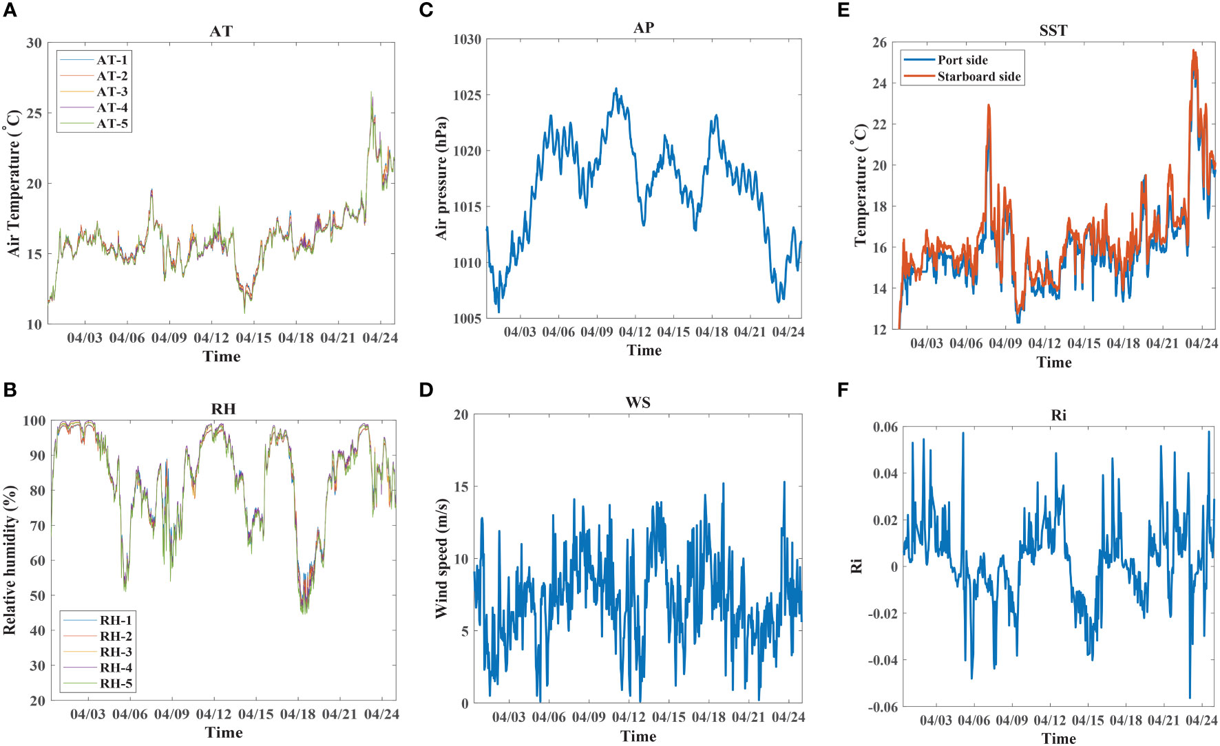
Figure 4 Variation curves of the acquired observation data in the time dimension. (A) AT; (B) RH; (C) AP; (D) WS; (E) SST; (F) Ri.

The profiles of AT and RH with height changed continuously over time. These changes are the main factor for the generation, development, and evolution of evaporation ducts. As shown in Figure 5, the RH profile was different on different days and at different times of the day. As shown in Figures 5A, B, the RH appears to decrease sharply at the highest level, and this change could easily cause the rapid generation of an evaporation duct. Figure 6 shows the change trend in the temperature profiles on different days and at different times of the day. The asterisk (“*”) at a height of 0 m indicates the SST. At some times, there were large variations in AT, up to 3° C. It can be seen from Figures 5, 6 that under different meteorological and hydrological environments, the AT and RH profiles are constantly changing, and this leads to constant changes in the evaporation duct.

FIGURE 5

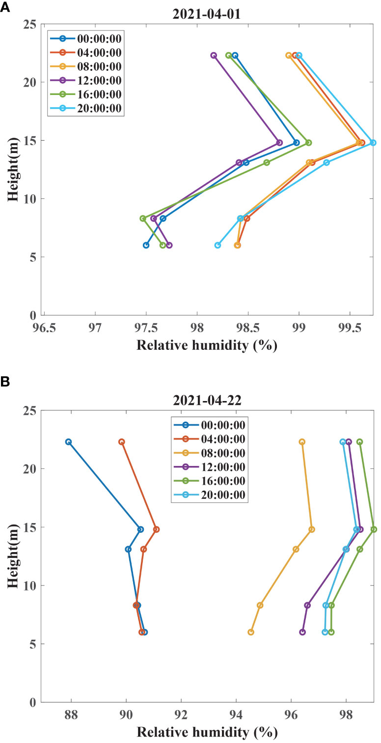
Figure 5 Change trends of the RH profile on different days and at different times of the day. (A) 01 April 2021; (B) 22 April 2021.

FIGURE 6

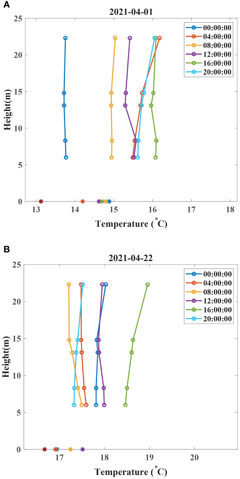
Figure 6 Change trends of the AT profile on different days and at different times of the day. (A) 01 April 2021; (B) 22 April 2021.

A statistical analysis of the observation data in the spatial dimension is shown in Figure 7. Figure 7A shows that the AT is generally lower in the north and higher in the south. The AT is the highest in the northeastern waters of Taiwan, where the Kuroshio approaches the coast of China. Figure 7B shows the changes in RH in the spatial dimension. It can be seen that during the voyage along the coast of China, the RH was relatively high; however, it varied greatly during the voyage. Figure 7C shows the changes in AP in the spatial dimension. A relatively high AP appeared near 30°N, and the lowest AP appeared in the northeastern waters of Taiwan. Figure 7D shows the changes in WS in the spatial dimension. It can be seen that the WS values in the areas far from the coast are obviously greater than those near the coast. Figure 7E shows the variation of SST in the spatial dimension. The distribution is random, but in the sea area of northeastern Taiwan, it is significantly higher than in other sea areas, which is consistent with the high-temperature characteristics of the Kuroshio (Ferrari, 2011). In addition, the SST values in the Taiwan Strait are also significantly higher than those in other sea areas. Figure 7F shows the variation of Ri in the spatial dimension. It can be seen that the unstable conditions mainly appear between 28°N and 30° N, and strong stable conditions appear in many places.

FIGURE 7

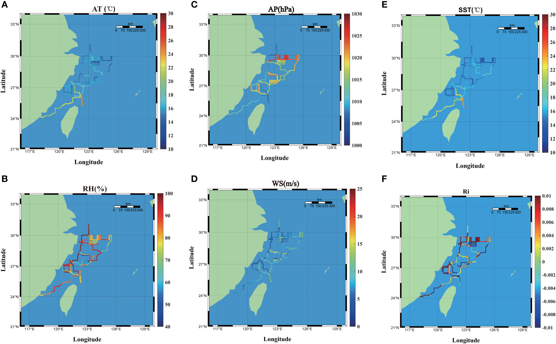
Figure 7 Statistical analysis of the observation data in the spatial dimension. (A) AT; (B) RH; (C) AP; (D) WS; (E) SST; (F) Ri.

At different moments, the M profile will continue to change with changes in the meteorological environment. Figure S2 shows the changes in the M profile every 2 h during the whole day on 5 April 2021. Changes in the M profile will inevitably cause the height of the evaporation duct to change. Figure S3 shows the change curve of the EDH on 5 April 2021. The EDH is lower at night and peaks at noon.

3.2. Analysis of EDM

Using the EDM, it is possible to directly obtain the refractive-index profile of the atmosphere using the WS , AT , RH , AP , and SST parameters of a single layer; the EDH can then be obtained according to the profile change rate. In different meteorological and hydrological environments, the atmospheric refractive-index profiles obtained from different models result in different values from that found at the observation height. As shown in Figure S4, under different meteorological and hydrological conditions, there are differences between the atmospheric refractive-index profile obtained by the model and the observed profile.

The differences in atmospheric refractive index in different layers and with different models in different environments were examined in terms of maximum absolute error (MAE), absolute average error (AAE), root-mean-square error (RMSE), and Pearson correlation coefficient (PCC). The results are shown in Table S1. The MAE values of NPS and NWA are better than those of other models. The AAE, RMSE, and PCC are all better, and the PCC in particular is close to 1, indicating that the overall trend predicted by the model is close to the observed value. It can also be seen that the deviations increase with increasing height. The NPS and NWA models showed better diagnostic results than the other models.

To further analyze the reason for the large values of MAE, the model diagnosis results were analyzed separately for different atmospheric stratifications. Tables S2, S3 show the analysis results under unstable and stable conditions, respectively. It can be seen from Table S2 that under unstable conditions, the deviations in atmospheric refractive index are small and the MAE values are relatively low. In contrast, Table S3 shows that the deviations in atmospheric refractive index are large under stable conditions. The large MAE values occur mainly under stable conditions.

To further analyze the factors affecting the accuracy of the model, the absolute deviations of the first-level M values were sorted in ascending order, and the factors causing these large deviations were analyzed. The results of this are shown in Figure 8. It can be easily concluded that when the M deviation is large, the corresponding Ri value is large and the WS is small, that is, under the conditions of low WS and strong stable conditions, the model’s diagnostic ability is poor.

FIGURE 8

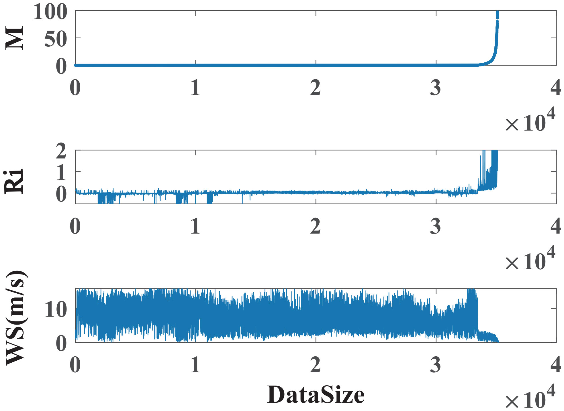
Figure 8 Relationship between the M deviation and Ri , as well as that between the M deviation and WS.

Therefore, we further analyzed the influence of different models on the diagnosis accuracy in different WS intervals under stable conditions. Figure 9A shows the maximum absolute error (M_max), average absolute error (M_mean), and root-mean-square error (M_rms) under stable conditions under all values (WS>0 m/s). According to M_max, it can be seen that the models BYC, NRL, and LKB have large diagnostic deviations in each layer. It can also be seen that the error increases with increasing layer height. Figure 9B shows the model diagnosis results when the atmosphere is under stable conditions and WS ≥3 m/s. It can be seen that, aside from the large deviation of NRL, the other models have high diagnostic accuracy. Figure 9C shows the model diagnosis results when the atmosphere is under stable conditions and WS≥5 m/s. It can be seen that the prediction accuracy of each model is high, and there is almost no difference between this diagnostic accuracy and that under unstable conditions. Furthermore, the accuracy is significantly higher than that for WS≥3 m/s.

FIGURE 9

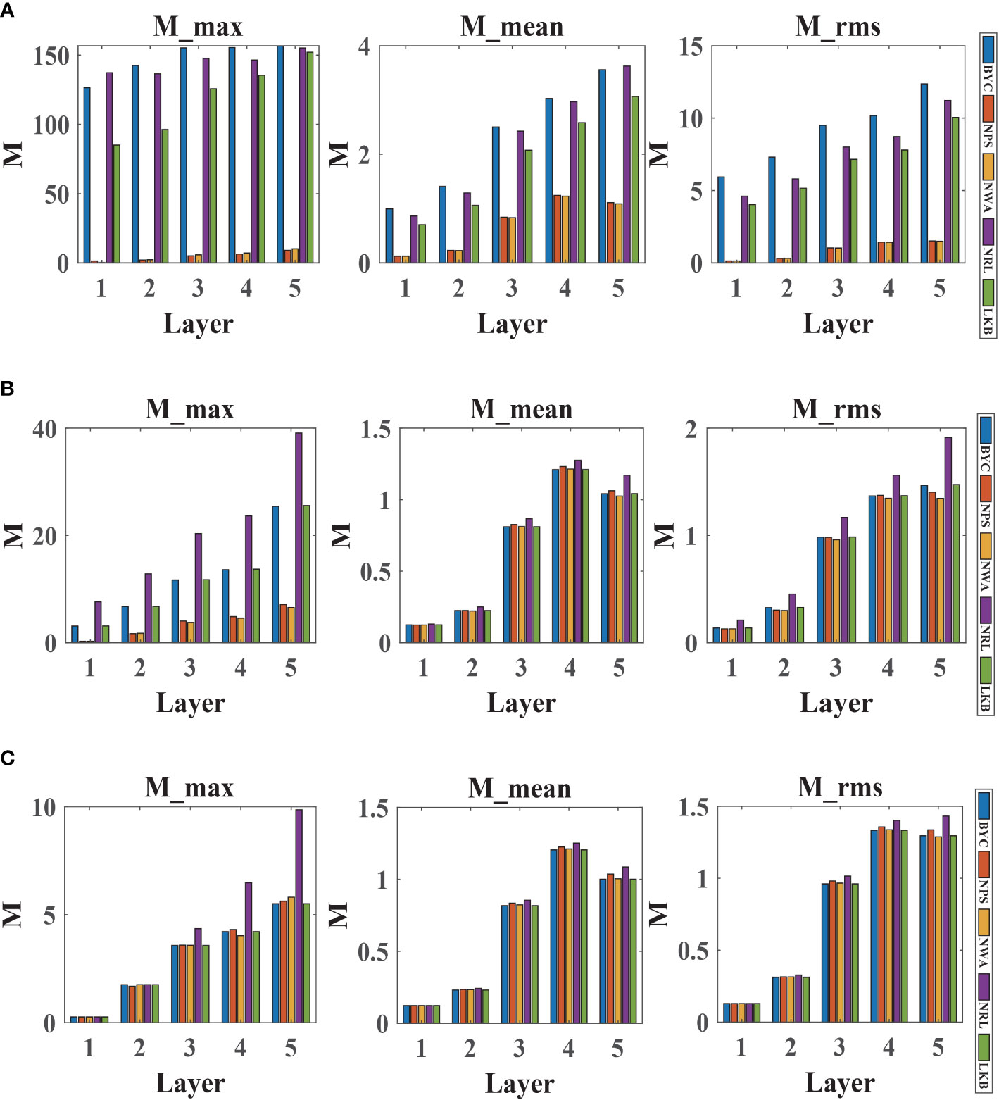
Figure 9 Model diagnosis results when the atmosphere is under stable conditions. (A) WS > 0 m/s. (B) WS ≥ 3 m/s. (C) WS ≥ 5 m/s.

From the above analysis, it can be concluded that each model has better diagnostic ability under unstable conditions, with almost no differences observed. However, under stable conditions, the diagnostic accuracy of the NPS and NWA models is better. Especially under strong stable conditions and low WS values, the prediction accuracy of the BYC, NRL, and LKB models is very low. However, when WS≥ 5 m/s, the prediction accuracy of each model increases. From this analysis of the observation data from the East China Sea on this voyage, it can be seen that the NPS and NWA models show better performance. Therefore, in Section 4, the NPS model is used to analyze the difference between the observation data and the reanalysis data with regard to evaporation ducts.

3.3. Comparative analysis of meteorological and hydrological data

To analyze the feasibility of using the reanalysis data to study the regional characteristics of evaporation ducts, the data quality of the ERA5 reanalysis data has been evaluated for the East China Sea based on the voyage observation data. Since the heights of the shipborne sensors are inconsistent with the heights used in the reanalysis data, we used the near-surface similarity theory to convert the heights of the reanalysis data into the heights of the observation data. The reanalysis data is grid point data with a horizontal resolution of 0.25°×0.25°, while the observation data is single point data. Therefore, we correspond to the grid point reanalysis data closest to the Euclidean distance from the single-point observation data.

A Taylor diagram was used to describe the standard error, RMSE, and correlations of the voyage observation data (WS, AT, RH, AP, and SST), and this is shown in Figure 10. Here, “Ship” represents the shipboard observation data, “ERA5” represents the ERA5 reanalysis data, and “CLDAS” represents the CLDAS reanalysis data. Figure 10A shows the WS comparison for ERA5, CLDAS, and the observation data. It can be seen that the values from ERA5 and CLDAS are close; the standard deviations are both greater than 2 m/s, the root-mean-square deviations (RMSD) are close to 2.5, and the correlations are 0.6. Figure 10B shows the AT data comparison. Overall, ERA5 is better than CLDAS, with a standard deviation of about 2°C. The correlation coefficients are both greater than 0.9. Figure 10C shows the RH data comparison. The accuracy of ERA5 and CLDAS is almost the same. Figure 10D shows the AP data comparison. CLDAS is better than ERA5, and the standard deviations are about 5 hPa. Since the CLDAS reanalysis data does not include SST, Figure 10E only compares ERA5 with the observation data in terms of SST. The standard deviation of the SST data of ERA5 is less than 2.5°C, the RMSD is less than 1.5° C, and the correlation coefficients are greater than 0.8. Through this analysis, it can be seen that the single parameters of the reanalysis data have high accuracy, and there are strong correlations with the observed data.

FIGURE 10

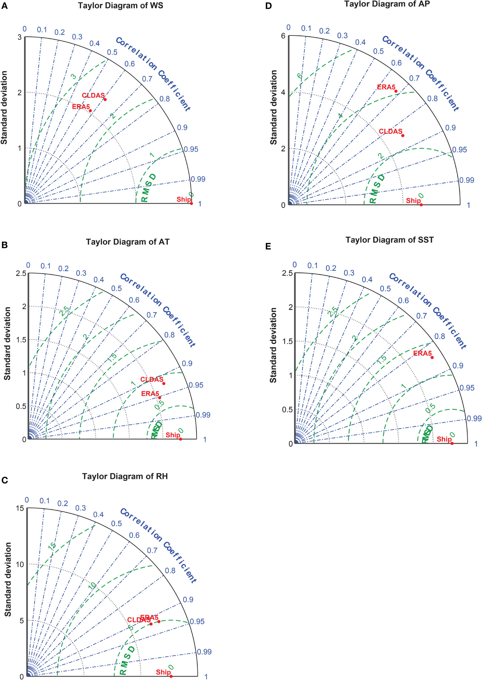
Figure 10 Accuracy of the reanalysis data: (A) WS; (B) AT; (C) RH; (D) AP; (E) SST.

4. Comparison and analysis of diagnosis results for evaporation ducts

As noted, meteorological and hydrological parameters at different heights were acquired through observations on this voyage. The height of the evaporation duct was diagnosed, and this was analyzed and compared with the values diagnosed by the NPS model using the ERA5 reanalysis data.

Using the EDM, the meteorological and hydrological parameters of the specified height were input. The EDH can then be calculated according to the Monin–Obukhov similarity theory. We used the 2-m AT, 2-m RH, 10-m WS, sea-surface AP, and the SST from the ERA5 datasets as the inputs of the EDM to obtain the EDH. Through the analysis in Section 3.2, it was found that the NPS model has strong applicability and high accuracy for the East China Sea; this model is thus adopted in this section. Therefore, the ERA5 reanalysis data was used as the input parameters for the NPS model, and the EDH was obtained. Then, a comparative analysis was made with the reference value of the EDH obtained from the voyage observation data. In this way, the feasibility of using the reanalysis data to examine the regional changes in evaporation ducts was obtained.

The analysis indicators in this paper were the false-report rate, the missing-report rate, the maximum diagnostic deviation, the average diagnostic deviation, the RMS of the diagnostic value, and the correlations under different atmospheric stratification. Figure S5 shows the change curves of the reference values of EDH obtained using the observation parameters during the voyage and the diagnostic values of EDH obtained by the NPS model using the reanalysis data. It can be seen that there is a strong correlation between the diagnostic values and the reference values, but there are also large deviations at some points in time.

False reports of evaporation ducts refer to a situation in which the reference value is 0 but the NPS diagnostic value is not 0. The false-report rate is the ratio of the number of false reports to the number of diagnoses. Missing reports refer to the situation in which the reference value is not 0 and the NPS diagnosis value is 0. Therefore, the missing-report rate is the ratio of the number of missing reports to the number of times the diagnostic reference value is not 0. The false- and missing-report results for evaporation ducts are shown in Tables 2, 3, respectively. It can be seen that the maximum false-report rate is only 3.24%, and the maximum missing-report rate is only 2.56% of the results obtained by reanalysis data, showing better diagnostic performance. At the same time, it can be seen that under the unstable conditions, the false-report rate is higher than that in other conditions, but under the unstable conditions, there is no missing report.

TABLE 2

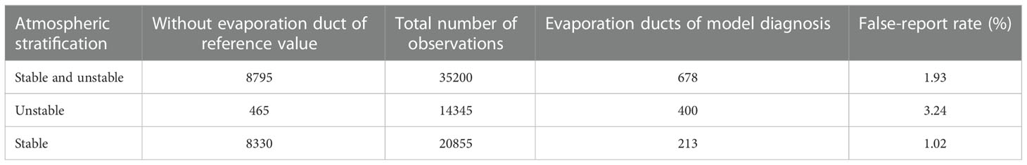
Table 2 Evaporation duct false-report results.

TABLE 3

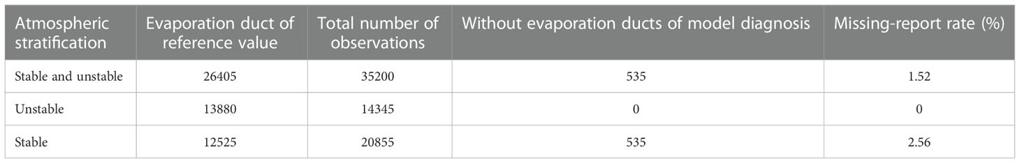
Table 3 Evaporation duct missing-report results.

Excluding false and missing reports of evaporation ducts, the maximum diagnosis deviation, average diagnosis deviation, RMS, and correlation coefficients between the reference and the diagnosis values were analyzed. The results are shown in Table 4. There is a large diagnostic bias in both stable and unstable conditions. However, diagnostic bias was acceptable and strongly correlated, as seen by the average diagnosis deviation, RMS, and correlation coefficients.

TABLE 4

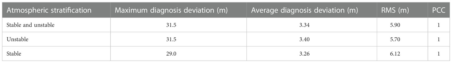
Table 4 Analysis of EDH diagnosis results.

Figure 11 shows the cumulative distribution functions (CDFs) of the deviation between the reference value and the diagnosis value. There are two kinds of input data for the EDH calculated by the NPS model: the meteorological parameters of each layer along with the sea-surface parameters obtained from the voyage, and the reanalysis data. Ship-true-1, 2, 3, 4, 5 represent the height difference between the reference value and diagnostic value by observation data of the 1, 2, 3, 4, and 5th floors ofthe ship, respectively. ERA5-true indicates the difference between the evaporative duct height diagnosed with the ERA5 dataset and the reference value. With increasing height, the deviations of the diagnosis results tend to gradually increase, but these deviations are slight. Regarding the reanalysis data, it can be seen that the results under unstable conditions are slightly better than those under stable conditions, although the differences are also small.

FIGURE 11

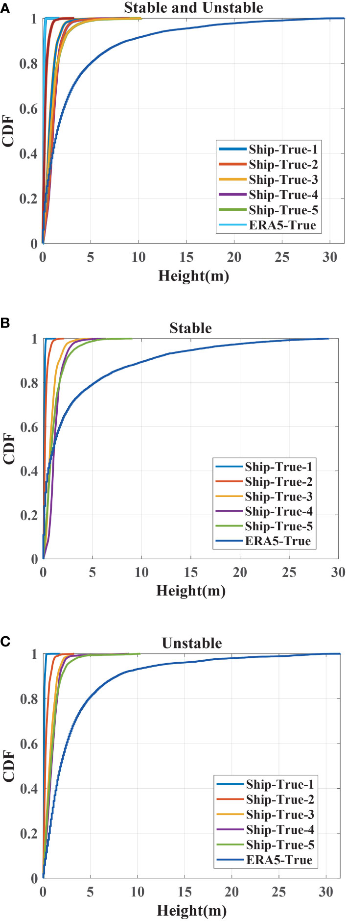
Figure 11 Diagnosis results showing the CDF of the EDH under different atmospheric stratifications: (A) stable and unstable conditions; (B) stable conditions; (C) unstable conditions.

From the above analysis, it can be concluded that it is basically feasible to analyze the characteristics of evaporation ducts based on the NPS model using the reanalysis data. The diagnosis accuracy is similar to that of the observational data using the EDM. The EDM diagnosis accuracy when using reanalysis data is close to that of using observation data.

5. Discussion and conclusion

In this work, we first analyzed the accuracy of different models under different meteorological and hydrological environments through layered observations from an actual voyage. It is concluded that the NPS model is better than the other models examined, regardless of whether the stratification of the atmosphere is stable or unstable.

From further analysis of the factors affecting the diagnostic accuracy of the model, it is concluded that when the M deviation increases, the corresponding Ri value increases and the WS decreases. This means that under conditions of low WS and strong stable conditions, the EDM has poor diagnostic ability. Additional analysis found that in different WS ranges, each model has better diagnostic ability under unstable conditions, with almost no differences observed. However, under stable conditions, the diagnostic accuracy of NPS and NWA is better than that of other models. Therefore, by analyzing the actual observation data, it was found that the NPS and NWA models show better performance in the East China Sea.

The ERA5 and CLDAS reanalysis data were compared with the observation data. It was found that the reanalysis data had consistent correlations with the observation data, and the errors are reasonable. The ERA5 reanalysis data and the observation data were then used as the inputs of the NPS model to obtain the EDH. The results show that the false-report rate of the model was highest under unstable conditions, but it was still only 3.24%. Under stable conditions, the missing-report rate was higher than under unstable conditions, at 2.56%. Regardless of the atmospheric stratification, the average diagnostic error was about 3 m. According to this analysis, it was concluded that the model diagnostic error of using the reanalysis data is similar to that obtained using actual observation data. It is thus reasonable and feasible to use reanalysis data to analyze the characteristics of evaporation ducts.

The analysis of this work was based on observation data from the East China Sea obtained in April 2021. Due to the difficulty of making marine observations, the observation period of this dataset was relatively long. However, in terms of scientific analysis, this quantity of data still leads to certain limitations. Therefore, in the future, more actual observational data from more sea areas and more seasons will continue to be obtained through more voyages. More buoys will be deployed, and platforms such as offshore observation towers will be applied to further verify our conclusions.

In addition, in combination with the existing observation data, we intend to analyze the underlying causes of the large deviations of the model. In view of different meteorological and hydrological conditions, the parameterization schemes for the atmospheric stability function and roughness should be improved. Different methods to improve the model are proposed to further increase the accuracy of the EDM.

Based on the conclusions of this paper, we will further research the evolution of evaporation ducts and the processes of their formation, development, growth, and extinction based on the reanalysis data for the East China Sea. The purpose of this is to reveal the underlying causes of the formation and development of evaporation ducts. We will also use numerical prediction methods to achieve short-term predictions of the EDH, and we will verify the feasibility and accuracy of this prediction method using voyage observation data.

Data availability statement

The raw data supporting the conclusions of this article will be made available by the authors, without undue reservation.

Author contributions

ZQ contributed to the conception and design of the study and the manuscript preparation. CZ performed the statistical analysis and wrote sections of the manuscript. BW, ZL, TH, JZ, SC, and SW contributed to the experiments. All authors contributed to manuscript revision, and they read and approved the submitted version.

Funding

The paper was supported by: the National Natural Science Foundation of China (Grant Nos. 42206188, 42076195, 42176185, and 41976179); the Natural Science Foundation of Shandong Province of China (Grant Nos. ZR2020QD085, ZR2020MF022, ZR2021MD114, and ZR2020MD058); the Computer Science Foundation of QLU (Grant Nos. 2021JC01001 and 2021JC02002); the Science, Education and, Industry Foundation of QLU (Grant No. 2022PYI004); and the Wenhai Program of QNLM (Grant No. 2021WHZZB0204).

Acknowledgments

Data acquisition and sample collection were supported by the National Natural Science Foundation of China Open Research Cruise (Cruise No. NORC2021-02+NORC2021-301), which is funded by the Shiptime Sharing Project of the National Natural Science Foundation of China. This cruise was conducted on board the R/V Xiangyanghong 18 by the First Institute of Oceanography, Ministry of Natural Resources, China. The ERA5 data used in this study can be retrieved from the following website: https://confluence.ecmwf.int/display/CKB/How+to+download+ERA5. The CLDAS data used in this study can be retrieved from the following website: http://data.cma.cn/data/cdcdetail/dataCode/NAFP_CLDAS2.0_RT.html. The authors would like to thank the reviewers for their careful work.

Conflict of interest

The authors declare that the research was conducted in the absence of any commercial or financial relationships that could be construed as a potential conflict of interest.

Publisher’s note

All claims expressed in this article are solely those of the authors and do not necessarily represent those of their affiliated organizations, or those of the publisher, the editors and the reviewers. Any product that may be evaluated in this article, or claim that may be made by its manufacturer, is not guaranteed or endorsed by the publisher.

Supplementary material

The Supplementary Material for this article can be found online at: https://www.frontiersin.org/articles/10.3389/fmars.2022.1108600/full#supplementary-material

References

Almond T., Clarke J. (1983). Consideration of the usefulness of microwave propagation prediction methods on air-to-ground paths. IEEE Proc. F 130, 649–656. doi: 10.1049/ip-f-1.1983.0098

CrossRef Full Text | Google Scholar

Babin S. M., Dockery G. D. (2002). Lkb-based evaporation duct model comparison with buoy data. J. Appl. Meteorol. Clim. 41, 434–446. doi: 10.1175/1520-0450(2002)041<0434:LBEDMC>2.0.CO;2

CrossRef Full Text | Google Scholar

Babin S. M., Young G. S., Carton J. A. (1997). A new model of the oceanic evaporation duct. J. Appl. Meteorol. Climatol. 36, 193–204. doi: 10.1175/1520-0450(1997)036<0193:ANMOTO>2.0.CO;2

CrossRef Full Text | Google Scholar

Burk S. D., Thompson W. T. (1989). A vertically nested regional numerical weather prediction model with second-order closure physics. Mon. Weather Rev. 117, 2305–2324. doi: 10.1175/1520-0493(1989)117<2305:AVNRNW>2.0.CO;2

CrossRef Full Text | Google Scholar

Chai X., Li J., Zhao J., Wang W., Zhao X. (2022). Lgb-phy: An evaporation duct height prediction model based on physically constrained lightgbm algorithm. Remote Sens. 14, 3448. doi: 10.3390/rs14143448

CrossRef Full Text | Google Scholar

Fairall C. W., Bradley E. F., Hare J. E., Grachev A. A., Edson J. B. (2003). Bulk parameterization of air–sea fluxes: Updates and verification for the COARE algorithm. J. Clim. 16, 571–591. doi: 10.1175/1520-0442(2003)016<0571:BPOASF>2.0.CO;2

CrossRef Full Text | Google Scholar

Ferrari R. (2011). A frontal challenge for climate models. Science 332, 316–317. doi: 10.1126/science.1203632

PubMed Abstract | CrossRef Full Text | Google Scholar

Frederickson P. A., Davidson K. L., Goroch A. K. (2000). Operational bulk evaporation duct model for MORIAH. tech. rep., naval postgraduate school. draft version.

Google Scholar

Haack T., Wang C., Garrett S., Glazer A., Mailhot J., Marshall R. (2010). Mesoscale modeling of boundary layer refractivity and atmospheric ducting. J. Appl. Meteorol. Climatol. 49, 2437–2457. doi: 10.1175/2010JAMC2415.1

CrossRef Full Text | Google Scholar

Hitney H., Vieth R. (1990). Statistical assessment of evaporation duct propagation. IEEE Trans. Antennas Propag. 38, 794–799. doi: 10.1109/8.55574

CrossRef Full Text | Google Scholar

Hodur R. M. (1997). The naval research laboratory’s coupled ocean/atmosphere mesoscale prediction system (COAMPS). Mon. Weather Rev. 125, 1414–1430. doi: 10.1175/1520-0493(1997)125<1414:TNRLSC>2.0.CO;2

CrossRef Full Text | Google Scholar

Jeske H. (1973). “State and limits of prediction methods, of radar wave propagation conditions over the sea,” in Modern topics in microwave propagation and air-Sea interaction (Dordrecht: Reidel Publishers), 131–148. doi: 10.1007/978-94-010-2681-9_13

CrossRef Full Text | Google Scholar

Jiao L., Zhang Y. (2015). An evaporation duct prediction model coupled with the MM5. Acta Oceanol. Sin. 34, 46–50. doi: 10.1007/s13131-015-0666-z

CrossRef Full Text | Google Scholar

Karimian A., Yardim C., Gerstoft P., Hodgkiss W. S., Barrios A. E. (2012). Multiple grazing angle sea clutter modeling. IEEE Trans. Antennas Propag. 60, 4408–4417. doi: 10.1109/TAP.2012.2207033

CrossRef Full Text | Google Scholar

Lentini N. E., Hackett E. E. (2015). Global sensitivity of parabolic equation radar wave propagation simulation to sea state and atmospheric refractivity structure. Radio Sci. 50, 1027–1049. doi: 10.1002/2015RS005742

CrossRef Full Text | Google Scholar

Liu W. T., Blanc T. V. (1984). The liu, katsaros, and businger, (1979) bulk atmospheric flux computational iteration program in FORTRAN and BASIC (Washington, DC: Tech. rep., Naval Research Laboratory).

Google Scholar

Liu W. T., Katsaros K. B., Businger J. A. (1979). Bulk parameterization of air-sea exchanges of heat and water vapor including the molecular constraints at the interface. J. Atmos. Sci. 36, 1722–1735. doi: 10.1175/1520-0469(1979)036<1722:BPOASE>2.0.CO;2

CrossRef Full Text | Google Scholar

Luo H., Ge F., Yang K., Zhu S., Peng T., Cai W., et al. (2019). Assessment of ECMWF reanalysis data in complex terrain: Can the CERA-20C and ERA-interim data sets replicate the variation in surface air temperatures over sichuan, China? Int. J. Climatol. 39, 5619–5634. doi: 10.1002/joc.6175

CrossRef Full Text | Google Scholar

Meng X., Guo J., Han Y. (2018). Preliminarily assessment of ERA5 reanalysis data. J. Mar. Meteorol. 38, 91–99. doi: 10.19513/j.cnki.issn2096-3599.2018.01.01110.19513/j.cnki.issn2096-3599.2018.01.011

CrossRef Full Text | Google Scholar

Qiu Z., Hu T., Wang B., Zou J., Li Z. (2022). Selection optimal method of evaporation duct model based on sensitivity analysis. J. Atmos. Ocean. Technol. 39, 941–957. doi: 10.1175/JTECH-D-21-0133.1

CrossRef Full Text | Google Scholar

Shi H., Cao X., Li Q., Li D., Sun J., You Z., et al. (2021). Evaluating the accuracy of ERA5 wave reanalysis in the water around china. J. Ocean. Univ. China 20, 1–9. doi: 10.1007/s11802-021-4496-7

CrossRef Full Text | Google Scholar

Shi Y., Zhang Q., Wang S., Yang K., Yang Y., Yan X., et al. (2019). A comprehensive study on maximum wavelength of electromagnetic propagation in different evaporation ducts. IEEE Access 7, 82308–82319. doi: 10.1109/ACCESS.2019.2923039

CrossRef Full Text | Google Scholar

Sun Z., Ning H., Tang J., Xie Y.-J., Shi P.-F., Wang J.-H., et al. (2016). Anomalous propagation conditions of electromagnetic wave observed over bosten lake, China in July and august 2014. Chin. Phys. B 25, 024101. doi: 10.1088/1674-1056/25/2/024101

CrossRef Full Text | Google Scholar

Tian B., Liu Q., Lu J., He X., Zeng G., Teng L. (2020). The influence of seasonal and nonreciprocal evaporation duct on electromagnetic wave propagation in the gulf of aden. Results Phys. 18, 103181. doi: 10.1016/j.rinp.2020.103181

CrossRef Full Text | Google Scholar

Wang J., Zhou H., Li Y., Sun Q., Wu Y., Jin S., et al. (2018). Wireless channel models for maritime communications. IEEE Access 6, 68070–68088. doi: 10.1109/ACCESS.2018.2879902

CrossRef Full Text | Google Scholar

Yang S., Li X., Wu C., He X., Zhong Y. (2017). Application of the PJ and NPS evaporation duct models over the south China Sea (SCS) in winter. PloS One 12, e0172284. doi: 10.1371/journal.pone.0172284

PubMed Abstract | CrossRef Full Text | Google Scholar

Zaidi K. S., Jeoti V., Drieberg M., Awang A., Iqbal A. (2018). Fading characteristics in evaporation duct: Fade margin for a wireless link in the south China Sea. IEEE Access 6, 11038–11045. doi: 10.1109/ACCESS.2018.2810299

CrossRef Full Text | Google Scholar

Zhang X., Liang S., Wang G., Yao Y., Jiang B., Cheng J. (2016b). Evaluation of the reanalysis surface incident shortwave radiation products from ncep, ecmwf, gsfc, and jma using satellite and surface observations. Remote Sens. 8, 225. doi: 10.3390/rs8030225

CrossRef Full Text | Google Scholar

Zhang Q., Yang K., Shi Y., Yan X. (2016a). “Oceanic propagation measurement in the northern part of the south China Sea,” in OCEANS 2016 (Shanghai: IEEE), 1–4.

Google Scholar

Zhang Q., Yang K., Yang Q. (2017). Statistical analysis of the quantified relationship between evaporation duct and oceanic evaporation for unstable conditions. J. Atmos. Ocean. Technol. 34, 2489–2497. doi: 10.1175/JTECH-D-17-0156.1

CrossRef Full Text | Google Scholar

Zhao Q., Haack T., McLay J., Reynolds C. (2016). Ensemble prediction of atmospheric refractivity conditions for EM propagation. J. Appl. Meteorol. Climatol. 55, 2113–2130. doi: 10.1175/JAMC-D-16-0033.1

CrossRef Full Text | Google Scholar

Zhu M., Atkinson B. W. (2005). Simulated climatology of atmospheric ducts over the Persian gulf. Bound.-Layer Meteorol. 115, 433–452. doi: 10.1007/s10546-004-1428-1

CrossRef Full Text | Google Scholar