Estimating sea spray volume flux with a laser gauge in a self-consistent system

Sea spray is one of the drivers of heat, mass, and gas exchange between the ocean and the atmosphere, and its volume flux could be estimated by the record of the laser intensity. In the laboratory experiments, the relationship between sea spray and laser intensity could be established since the returned laser intensity of the observing gauge and spray concentration can be observed instantaneously. However, the difficulty to generalize the laboratory result to field observations is that the measurement of sea spray is usually unavailable on the open seas. Recent studies introduced an environment variable (atmospheric extinction coefficient for instance) to relate the laser intensity to spray volume flux for both laboratory and field observations so that the relationship established in the laboratory experiments could be extended to open seas. These studies however gave estimations of great difference since the relationships between each pair of the variables (spray volume flux, laser intensity, and the atmospheric extinction coefficient) are considered separately. This work established a self-consistent system composed of the three variables, in which the relationship between each pair of the variables in the system is consistent with that deduced from their respective relationships with the third variable. Consistency here we means that if Y=f(X), Y=g(Z) and Z=h(X), then Y=g(h(X))=f(X) is expected. The consistency of the relationships ensures that the estimation of the sea spray volume flux from laser intensity is robust. We established self-consistent relationships for the variables in the system composed of laser intensity, environment variable, and sea spray volume flux, for both laboratory and field experiments. Among them, the relationship between wind speed and spray volume flux is a reasonable reflection of the physical properties in two ways: a threshold value of spray volume flux at low wind speeds and the saturation at strong wind speeds. For a uniform regression of wind speed onto spray volume, a dimensionless parameter concerning wind speed is needed.

1. Introduction

Sea spray (or ocean spray) droplets are generated through bubble bursting, tearing off of spume drops by wind from sea surface waves, and other minor mechanisms (Veron, 2015). Blowing over the ocean surface, the wind generates sea spray droplets whose sizes vary from the order of nanometers to several millimeters (Veron, 2015). At the ocean surface, sea spray contributes to the exchange of latent heat (Andreas, 1992; Andreas, 2004; Shi and Xu, 2022), water vapor, and momentum between the atmosphere and the ocean (Andreas et al., 1995; Andreas, 1998; Melville and Matusov, 2002). Large spray droplets that fall onto the ocean after suspending some time in the lower atmosphere can affect the thermodynamics and intensity of tropical storms (Fairall et al, 1994; Andreas, 2002; Emanuel, 2003; Haus et al., 2010; Bao et al., 2011; Bianco et al., 2011; Soloviev et al., 2014; Takagaki et al., 2016; Zhao et al., 2017; Troitskaya et al., 2018).

During the past decades, laboratory and field experiments have been conducted to estimate the sea spray concentration and establish parameterizations of the sea spray volume flux (Andreas, 1998; O’Dowd and de Leeuw, 2007). Early studies focus on the development of the sea spray generation function (SSGF) for spray droplets through observations. Monahan et al. (1986) suggested SSGFs based on the coverage rate of whitecaps or the wind speed at 10 m above the ocean surface (U₁₀). Iida et al. (1992) introduced an SSGF as a function of friction velocity, the kinematic viscosity of air, and the peak angular frequency of the wind-wave part of wave spectra. Zhao et al. (2006) proposed an SSGF for spray droplets based on the wind sea Reynolds number. However, empirical spray generation functions describing the size spectra of spray can differ by up to six orders of magnitude (Troitskaya et al., 2018). Since measurements of sea spray concentration are hard to perform in the open seas, most of the SSGFs remain uncertain for high wind conditions, especially during tropical storms (Emanuel, 1995; Anguelova et al., 1999).

In a laboratory setup, Toffoli et al. (2011) found a relationship between the sea spray volume flux and the intensity of the returning signal of a down-looking laser sensor, allowing, in principle, the estimation of spray volume fluxes in case of no wind observation. In the open seas, however, the optical technique to estimate the spray concentration, which was employed in Toffoli et al. (2011), is usually difficult to perform. Therefore, the estimation of spray volume flux by taking advantage of a laser gauge is then of great significance. The generalization of Toffoli et al.’s approach (2011) to the field is challenging since the laser intensity also depends on experimental conditions (the distance from the laser gauge to the water surface, for instance).

Sea spray affects the attenuation of laser intensity (P) by changing the atmospheric extinction coefficient (γ) or the laser attenuation coefficient (μ). To establish a relationship between sea spray volume flux (V) and γ/μ that applies to both laboratory and field observations, a practical way is to start from Toffoli et al.’s laboratory observations on spray volume and laser intensity. It is just the starting point for both Ma et al. (2020) and Xu et al. (2021). By introducing the atmospheric extinction coefficient γ, Ma et al. (2020) related the laser intensity to spray volume flux and extended the method of Toffoli et al. (2011) for the field observations. In almost the same way, Xu et al. (2021) also related the laser intensity to spray volume flux by introducing the laser attenuation coefficient μ. These two studies followed the same idea but yielded quite different estimations of sea spray volume flux.

In a ternary system composed of spray volume flux V, laser intensity P, and atmospheric extinction coefficient γ (or laser attenuation coefficient μ), the relationships between each pair of them should be consistent. That is, if V=f(γ), V=g(P) and P=h(γ), then V=g(h(γ))=f(γ) is expected. However, those studies considered the relationships between each pair of the variables separately regardless of their consistency as a whole. In this work, we establish self-consistent relationships in the ternary system. A robust relationship between sea spray volume flux and laser intensity is then established. Sea spray volume flux can also be estimated by wind speed directly.

2. Materials and methods

In this work, we use both the laboratory observations in Toffoli et al. (2011) and the field data used in Ma et al. (2020).

2.1. Laboratory observations

Experimental data are from Toffoli et al. (2011). They conducted laboratory tests in the air-sea interaction tank of the University of Miami, with dimensions 15 m×1 m×1 m, to capture the spray volume passing through a specific cross section in extreme wind conditions, wind speed (U₁₀) between 20 and 60 m s^-1 with increments of 5 m s^-1. Spray volume was measured directly with image processing techniques using a Digital Laser Elevation Gauge that illuminated a portion of the air-sea interface and a digital line scan camera (see details in Toffoli et al., 2011). A down-looking Optech Sentinel 3100 laser gauge installed 1.2 m above the still water surface was used to measure the returning laser intensity (the intensity of the laser signal backscattered by the rough water surface and passing through suspended spray particles).

Based on the laboratory measurements, Toffoli et al. (2011) derived an empirical model correlating spray volume with laser intensity:

$\begin{array}{ll}V=-3\times {10}^{-10}{P}^2+5\times {10}^{-7}P-8\times {10}^{-5}& (1)\end{array}$

where V is spray volume, and P is the returned laser intensity of the observing gauge (Figure 1A).

FIGURE 1

Figure 1 Relationships of laser intensity, sea spray volume flux, and wind speed for laboratory experiment in Toffoli et al. (2011) (A); Sketch of mapping of laser intensity onto the environment variable (γ in Ma et al., 2020, or μ in Xu et al., 2021) (B); The approaches to estimating spray volume flux by laser intensity, Ma et al. (C), and Xu et al. (D). For field observations, both Ma et al. and Xu et al. mapped laser intensity onto an environment variable first and then estimated the spray volume flux from laser intensity with the help of the environment variable. Solid arrows in (A, C, D) indicate that an analytic relationship between the two variables has been established, while hollow arrows indicate that the relationship between the two variables has not been established. Blue arrows for field observations and green arrows for laboratory observations. Hollow arrow with question mark is the major relationship to be established in the corresponding work.

2.2. Field observations

Field data were collected at a platform on the Northwest Shelf of Western Australia where the water depth is 125 m (see Babanin et al., 2016, for detail). Two ultrasonic anemometers were installed on a vertical cable above mean sea level to measure wind speed. A rectangular array of four Optech Sentinel 3100 laser gauges (of the same type as that employed in Toffoli et al., 2011) was fixed at 26.5 m above the mean sea level to measure the water surface elevation and the returned laser intensity. The observations covering a period from January to October 2015 are discussed in detail in Xu et al. (2021). Ma et al. (2020) provided further details for the tropical cyclone Olwyn, which was during 11–13 March 2015.

3. Results

3.1. Estimating sea spray volume flux from laser intensity

The atmospheric extinction coefficient (γ) could be used to relate sea spray to laser intensity (P). The relationship between P and γ is established by the rangefinder equation (Wojtanowski et al., 2014):

$\begin{array}{ll}P\left(R\right)=P_0\text{exp}\left(-2\gamma R\right)& (2)\end{array}$

where R is the distance from the laser gauge to the object, P₀ =Q₀ρA₀η₀/(πR²) , Q₀ is the output power of the transmitted laser pulse, A₀ the receiving aperture area, η₀ the receiving optics spectral transmission and ρ a parameter that depends only on the environmental conditions in the experiments.

For the laboratory observations (Figure 1B), Ma et al. (Figure 1C) mapped P onto γ first through Equation 2. They then related the derived atmospheric extinction coefficient to the observed spray volume in form of a polynomial function:

$\begin{array}{ll}V=-5\times {10}^{-3}{\text{γ}}^2+1.5\times {10}^{-3}\text{γ}& (3)\end{array}$

Note that the atmospheric extinction coefficient is a feature of the atmosphere itself and does not depend on the laser intensity. The relationship between V and γ then should not vary between laboratory and open seas, and the relationship established from laboratory data (Equation 3) therefore also applies to field data. Combining Equations 2 and 3, V can then be estimated from P by eliminating γ. The environmental parameters (P₀ and R) in the relationships vary in laboratory and field observations.

Xu et al. (Figure 1D) mapped laser intensity onto laser attenuation coefficient (μ) by Beer-Lambert law:

$\begin{array}{ll}P\left(R\right)=I_0\text{exp}\left(-2\mu R\right)& (4)\end{array}$

where I₀ is the base-level laser intensity. Regression of spray volume flux onto laser attenuation coefficient is then as follows:

$\begin{array}{ll}V\left(\mu \right)=2.80\times {10}^3{\mu }^{6.13}& (5)\end{array}$

It is also applicable for both laboratory and field observations as Equation 3 does since enviromental influence has been included in Equation 4. Eliminating μ in Equations 4 and 5, V can be estimated from P, which is different from Equation 1 since environmental factors (I₀ and R) are included as parameters in the relationship. Note that the rangefinder equation (Equation 2) is a special form of the Beer-Lambert law (Equation 4), meaning that the approaches in Ma et al. (2020) and Xu et al. (2021) are essentially the same. In another word, there is no essential difference between γ and μ. In the following discussion, we will still use both of the symbols when comparing the methods of Ma et al. (2020) with Xu et al. (2021).

The initial parameter P₀ of laser gauge in Equation 2 decreases with the laser-object distance (and so does the base-level laser intensity I₀ in Equation 4). Therefore, the maximum P in a field experiment is always no greater than that in a laboratory experiment, because the laser-object distance in a field experiment is greater than that in a laboratory experiment. As a consequence, the range of the mapping of P onto γ/μ for field observations is always a subset of that for laboratory observations. It ensures that the mapping of γ/μ onto V for field observations is defined on a subset of that for laboratory observations.

Sea spray volume flux estimated by Ma et al. (2020) is much greater than that by Xu et al. (2021), which is caused by two reasons. In the first instance, the value domains of γ and μ are different in the two methods. Xu et al. (2021) noticed that, in the field, a lot of spray is concentrated below the crests in the air gaps between the crests, and the concentration of spray there is much higher than above the crests. As a result, this region significantly affects the returned laser intensities, if not corrected for the difference. In the laboratory, because the wave heights are small, this difference is not noticeable at all, as at strong wind spray is mixed in the air columns near the surface, and the concentration is the same above and below the crests. In the field, however, when the waves are large, i.e. ~10 m, this difference affected the laser intensities in a significant way. Therefore, Xu et al. (2021) chose a different base level of laser intensity in their mapping of P onto μ (Equation 4) than that in Ma et al.’s (2020) mapping of P onto γ (Equation 2). In Ma et al. (2020), laser intensity ranges between 1050 and 1500 (P₀ = 1500 W m^-2) for the laboratory observations by Toffoli et al. (2011), and between 232.4 and 1247.6 (P₀ = 1247.6 W m^-2) for the field observations; In Xu et al. (2021), it ranges from 1200 to 1742 (I₀ = 1742 W m^-2) for the laboratory observations and 100 to 1400 (I₀ = 1400 W m^-2) for the field observations (Table 1).

TABLE 1

Table 1 Ranges of Laser Intensity in the Laboratory and Field Observations (unit: W m^-2).

The different domains of laser intensity and the selection of P₀/I₀ yield γ and μ of different ranges (Figure 1B). Figure 2 gives γ and μ as a function of wind speed. For laboratory experiments (wind speed ranges between 20 and 60 m s^-1), γ is less than μ when wind speed is over 45 m s^-1 and greater than μ when wind speed is below 45 m s^-1 (Figure 2A). For field experiments (wind speeds are between 5.0 and 22.7 m s^-1), γ is systematically, but not markedly, greater than μ (Figure 2B).

FIGURE 2

Figure 2 Values of the environment variable (γ in Ma et al., 2020, or μ in Xu et al., 2021) that derived from laser intensity for the laboratory (A) and field (B) experiments, respectively.

As we mentioned above that γ and μ are essentially the same parameter. However, Ma et al. and Xu et al. fit different regression models of γ or μ onto V (Figure 3). It is the second and more important reason for the difference in the results of the two studies. The mapping of P onto γ/μ in the laboratory (see Figure 1B) is the domain of γ/μ that derives spray volume flux by the regression models (Equations 3 and 5). In Ma et al.’s regression model, the response (output) variable V is derived from Toffoli’s regression model (Equation 1); While in Xu et al., observations of Toffoli et al. (2011) are utilized directly to derive a regression of μ onto V (Equation 5). As a consequence, sea spray volume flux in Ma et al. is a quadratic function of γ, and that in Xu et al. is in proportionate to μ^6.13. Since V in Toffoli et al.’s (2011) regression model decreases sharply with the increase of laser intensity, it also increases sharply concerning γ. The blue curves in Figure 3 show the estimated V from Ma et al. (by Equation 3) and Xu et al. (by Equation 5), respectively. Ma et al. (2020) fitted better on larger V while Xu et al. (2021) fitted better on smaller V. V derived from γ (Equation 3) is two or three orders greater than that derived from μ of the equal value as γ (Equation 5).

FIGURE 3

Figure 3 Regressions of spray volume flux onto γ and μ for the laboratory observations. The blue part of the regression line is in the range of γ or μ corresponding to the laser intensity in the field observations (calculate from Equations 3, 5, respectively).

3.2. Estimating the sea spray volume flux in a consistent system

For a system of three variables (a ternary system), there could be three relationships, each relating a pair of them. If the system is self-consistent, the relationship between each pair of them should also be deduced from the other two relationships concerning the third variable. In Ma et al. (2020), there are analytic relationships between P and γ (Equation 2), and between γ and V (Equation3). Eliminating γ in these two equations, we can deduce a regression from P onto V. This regression is in a different form than their direct relationship deduced by Toffoli et al. (Equation 1). That is, the three relationships (between P, γ, and V) in Ma et al. (2020) are not self-consistent. So does the relationships between variables in Xu et al. (2021). In this paper, we will establish a self-consistent system composed of spray volume flux, laser intensity, and environment variable (γ).

We start with the spray volume flux, laser intensity in the laboratory observations (Toffoli et al., 2011), and the atmospheric extinction coefficient γ derived from the laser intensity. In Toffoli et al.’s (2011) observations, the laser intensity grows monotonically as a whole with the increase of wind speed. An exception is for the laser intensity corresponding to wind speed at 35 m s^-1. We correct P corresponding to wind at 35 m s^-1 to the average of those corresponding to wind at 30 m s^-1 and 40 m s^-1, which is still in the 95% confidence intervals. Later we will reveal that the correction does not influence our results.

The previous discussion has shown (Figure 1B) that the laser intensity in the field observations has a different value range than that in laboratory observations and its mapping on γ in field observations is a subset of that in laboratory observations. Now we estimate the subset of γ, and then the corresponding range of P by using the parameters listed in Table 1.

For a given distance from the laser gauge to object (R), the returned laser intensity (P) decreases monotonically with the increase of atmospheric extinction coefficient (γ), as described in the rangefinder equation (Equation 2) and also sketched in Figure 1B. Therefore, the upper limit of γ in the relationship for the field experiment (R=26.5 m, P₀ = 1247.6 W m^-2) corresponds to the minimum P (=232.4 W m^-2, as listed in Table 1), so that

$${\gamma }_f{\_}_{max}=\text{ ln}\left(232.4/1247.6\right)/\left(-2\times 26.5\right)=0.0317\left({\text{m}}^{-1}\right)$$

where the subscript f stands for the field experiment.

Apply the rangefinder equation (Equation 2) to the laboratory parameters (R=1.29 m, P₀ = 1500 W m^-2), the minimum P corresponding to γ_{f_max} is

$$P_l{\_}_{min}=1500·\text{exp}(-2\times 1.29{\gamma }_f{\_}_{max})=1382\left(\text{W }{\text{m}}^{-2}\right)$$

where the subscript l stands for laboratory experiment.

In Toffoli et al. (2011), there are only four records of P being greater than P_{l_min}. These are the laser intensities that play roles in the relationship between V and γ, by determining the domain of γ. According to the rangefinder equation, we have

$\begin{array}{ll}\text{γ}=-\text{ln}\left(P/P_0\right)/\left(2R\right)& (6)\end{array}$

In the discussions hereinafter, we follow four rules when fitting a regression model between variables. Firstly, the regression model should be an elementary function. Secondly, the regression model should be a continuously differentiable function as a whole, that is, piece-wise regression will not be considered. Thirdly, the regression model should be monotonous over the predictor (input variable) domain so that we can find its inverse function. In other words, the input function could also be expressed as a monotonous function of output variables. This rule excluded the polynomial regressions. And lastly, if the output variable has a threshold value in its physical reality, the regression function should have an asymptotic line accordingly. So that the regression function is a proper approximation for the physical relationship, or have a better generalization performance for the values of response variable near the threshold.

We then move to the relationship between γ and V. Note that V varies over a range between 10^-7 and 10^-4. If we regress V directly onto γ, larger values will dominate the residue. Therefore, we take the natural logarithm of V as the output variable, and regress lnV onto γ:

$\begin{array}{ll}\text{ln}V=129\text{γ}-15.14& (7)\end{array}$

The R-square statistic of the regression is 0.99, meaning that 99% of the variability in lnV can be explained by using γ.

Equations 6 and 7 indicate that lnP is linearly correlated with lnV. Therefore, we regress lnV directly onto lnP:

$\begin{array}{ll}\text{ln}V=-50·\text{ln}P+350.50& (8)\end{array}$

The R-square statistic of the regression is 0.99, and the model satisfies our expectation for larger laser intensity data (P > 1360 W m^-2). Figure 4 suggests that although the regression model used corrected laser intensity, it is also a solid regression model of P without correction, as long as the linear relationship between lnV and lnP is concerned.

FIGURE 4

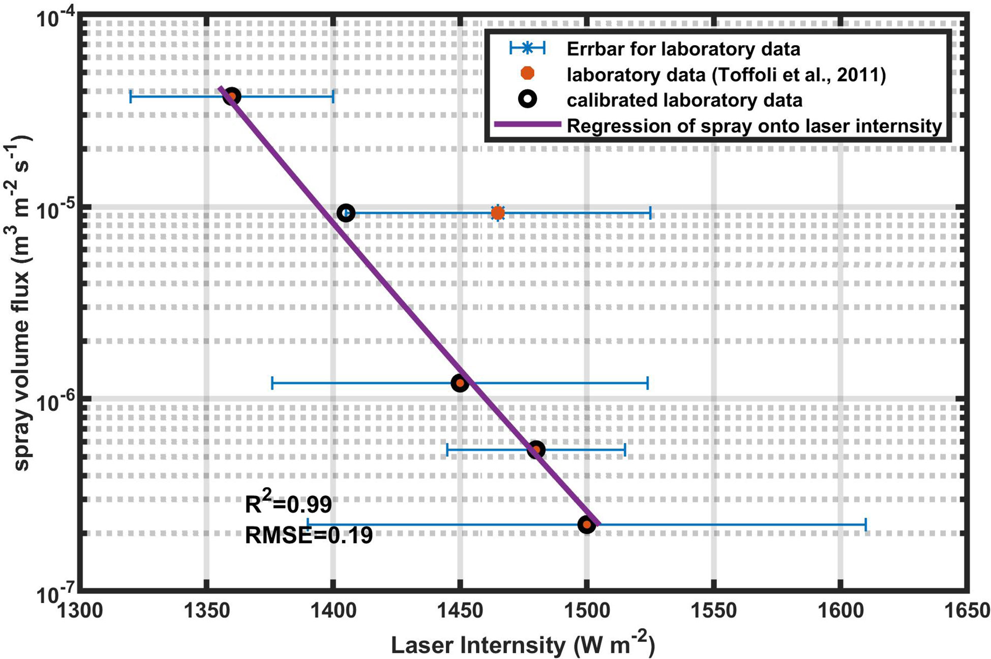
Figure 4 Regression of spray volume flux onto the laboratory laser intensity greater than 1360 W m^-2 (Equation 8). Orange stars and their error bars are the observations in Toffoli et al. (2011), and black circles are the data used in the regression.

Equation 8 is a direct regression of lnP on lnV from the observations in Toffoli et al. (2011). We can also deduce a similar relationship between lnP and lnV by eliminating γ in Equations 6 and 7:

$$-\text{ln}\left(P/P_0\right)/\left(2R\right)=\left(\text{ln}V+15.14\right)/129$$

It can be written in another form where lnV is a linear function of lnP:

$\begin{array}{ll}\text{ln}V=-\frac{129}{2\text{R}}·\text{ln}P+\left[\frac{129}{2\text{R}}·\text{ln}{P}_0-15.14\right]& (9)\end{array}$

For laboratory experiment in Toffoli et al. (2011), P₀ = 1500 W m^-2 and R=1.29 m. Equation 9 then yields

$\begin{array}{ll}\text{ln}V=-50·\text{ln}P+350.52& (10)\end{array}$

It is almost the same equation as Equation 8, indicating that we have established a self-consistent ternary system for partial laboratory observations (P > 1360 W m^-2). In this system, γ is a linear function of lnP (Equation 6) or lnV (Equation 7), and lnV is a linear function of lnP (Equation 8).

The relationship between P and γ (Equation 6), and that between P and V (Equation 9) all depend on environmental factors (P₀ and R), while the relationship between V and γ does not. That’s why the regression of V onto γ (Equation 7) also applies to field observations. Replacing environmental parameters R and P₀ in Equation 9 with those in field observation, we have

$\begin{array}{ll}\text{ ln}V=-\frac{129}{2\times 26.5}·\text{ln}\left(P\right)+\left[\frac{129}{2\times 26.5}·\text{ln}\left(1247.6\right)-15.14\right]=-2.43·\text{ln}P+2.21& (11)\end{array}$

It is an estimate of the sea spray volume flux in the field experiment by the laser intensity. The estimated sea spray volume flux against the wind speed is shown in Figure 5. The blue circles show that the estimated sea spray volume fluxes are smaller than Ma et al.’s (2020) estimation and greater than Xu et al.’s (2021) estimation. Compared with the results estimated by traditional methods (Monahan et al., 1986; Iida et al., 1992; Fairall et al., 1994; Andreas, 1998; Zhao et al., 2006; Troitskaya et al., 2018), sea spray volume fuxes estimated by Equation 11 decreases sharply to a threshold value at low wind speed (less than 5 m/s) and increases to a saturated state at wind speed (greater than 30 m/s).

FIGURE 5

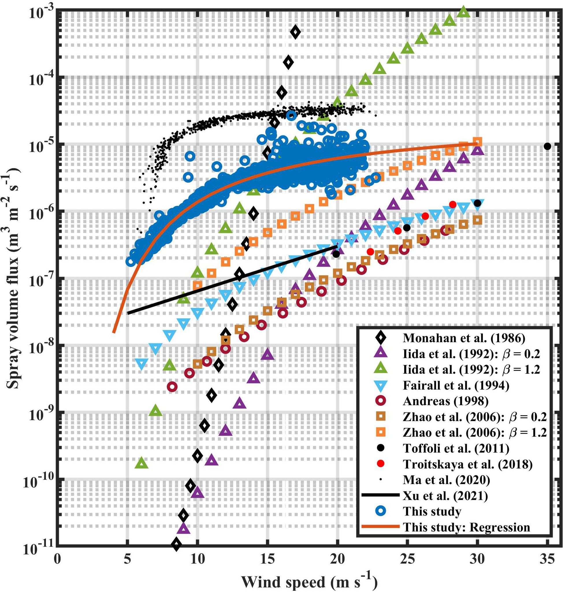
Figure 5 Spray volume flux against wind speed. Blue circles are the results of this study for the field observations. Monahan et al. (1986); Iida et al. (1992); Fairall et al. (1994), D. Zhao et al. (2006); Toffoli et al. (2011); Troitskaya et al. (2018); Ma et al. (2020) are also given for comparison. The black solid line represents an approximation of Xu et al. (2021).

Hence we have established self-consistent relationships for the variables in the system composed of laser intensity (P), environment variable (γ), and sea spray volume flux (V), for both laboratory and field experiments. Notice that the surface roughness is different for different wind speeds and that roughness affects the laser backscatter, not just spray attenuation. It can be a source of error. However, as Xu et al. (2021) mentioned, both roughness and spray volume would reduce the laser reflected intensity, and hence, in a way, they are correlated and the laser attenuation can be treated as a proxy for both connected properties: surface roughness and spray volume.

4. Discussion

We noticed that the estimated spray volume fluxes by laser intensity (Figure 5) concentrate around a regular curve line against wind speed, so we can further regress spray volume flux onto wind speed. Note also that lnV decreases with the increase of wind speed, we strive for a relationship between lnV and inverse wind speed (1/W), and get the following regression model:

$\begin{array}{ll}\text{ln}V=-29.2/W-10.56& (12)\end{array}$

The R-square statistic of this model is 0.90. The regression curve is also shown in Figure 5. The relationship between W and V (Equation 12) is a reasonable reflection of the physical properties in two ways. Firstly, V decreases sharply when W drops from 5 m s^-1 to 2 m s^-1. It is O(10^-8) at a wind of speed 5 m s^-1 and decreases to O(10^-11) at a wind speed of 2 m s^-1. It is natural to assume that there is no spray volume flux for lower wind (less than 2 m s^-1). Secondly, there is a saturated V with the increase in wind speed. The upper limit of V is 2.6×10^-5 when the wind speed increases to infinity.

Note that both 1nV and 1nP are linearly correlated with γ (Equations 6 and 7), and 1nV is also linearly correlated with 1/W (Equation 11), we expect to find a linear relationship between 1nP and 1/W. A regression model in this form is

$\begin{array}{ll}\text{ln}P=12/W+5.25& (13)\end{array}$

The R-square statistic of the model is 0.90. It is a good regression of lnP onto W (see Figure 6), not only in the statistical sense but also in the physical implication. Returned laser intensity should decline with the increase of wind speed. This relationship between inverse wind speed and laser intensity satisfies our expectations.

FIGURE 6

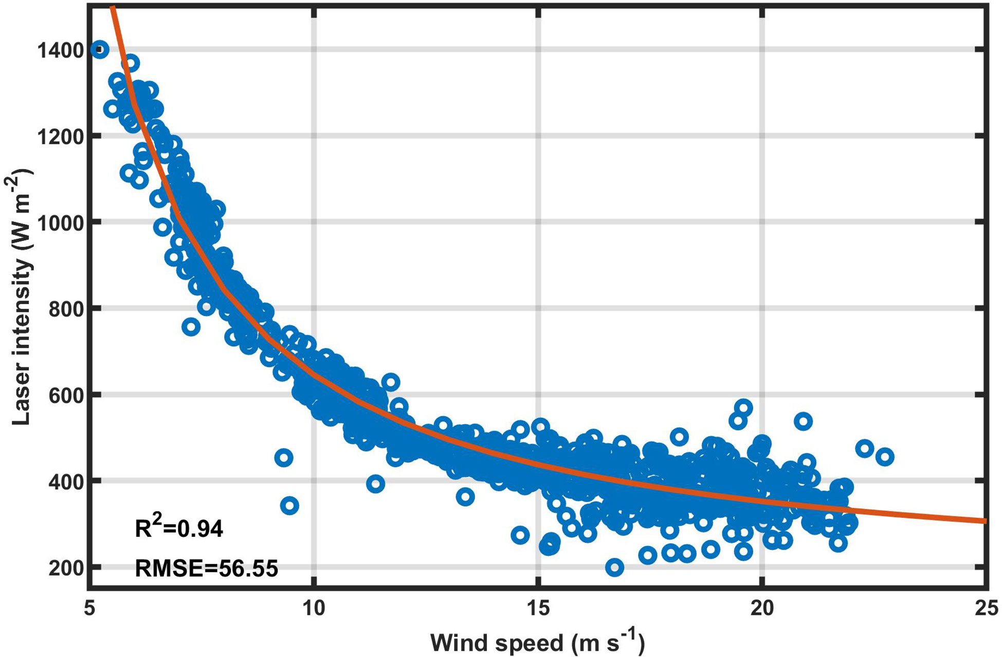
Figure 6 Laser intensity as a function of wind speed for the field observations (blue dots), and the regression (Equation 13) of laser intensity onto wind speed (red line).

We expect that the relationships for variables in laboratory experiments should be similar to those in field experiments. To verify the robustness of the relationships between sea spray volume flux and wind speed or laser intensity (Equations 12 and 13) for field observations, we try a linear regression model (see Figure 7) between lnV and 1/W for the laboratory data:

FIGURE 7

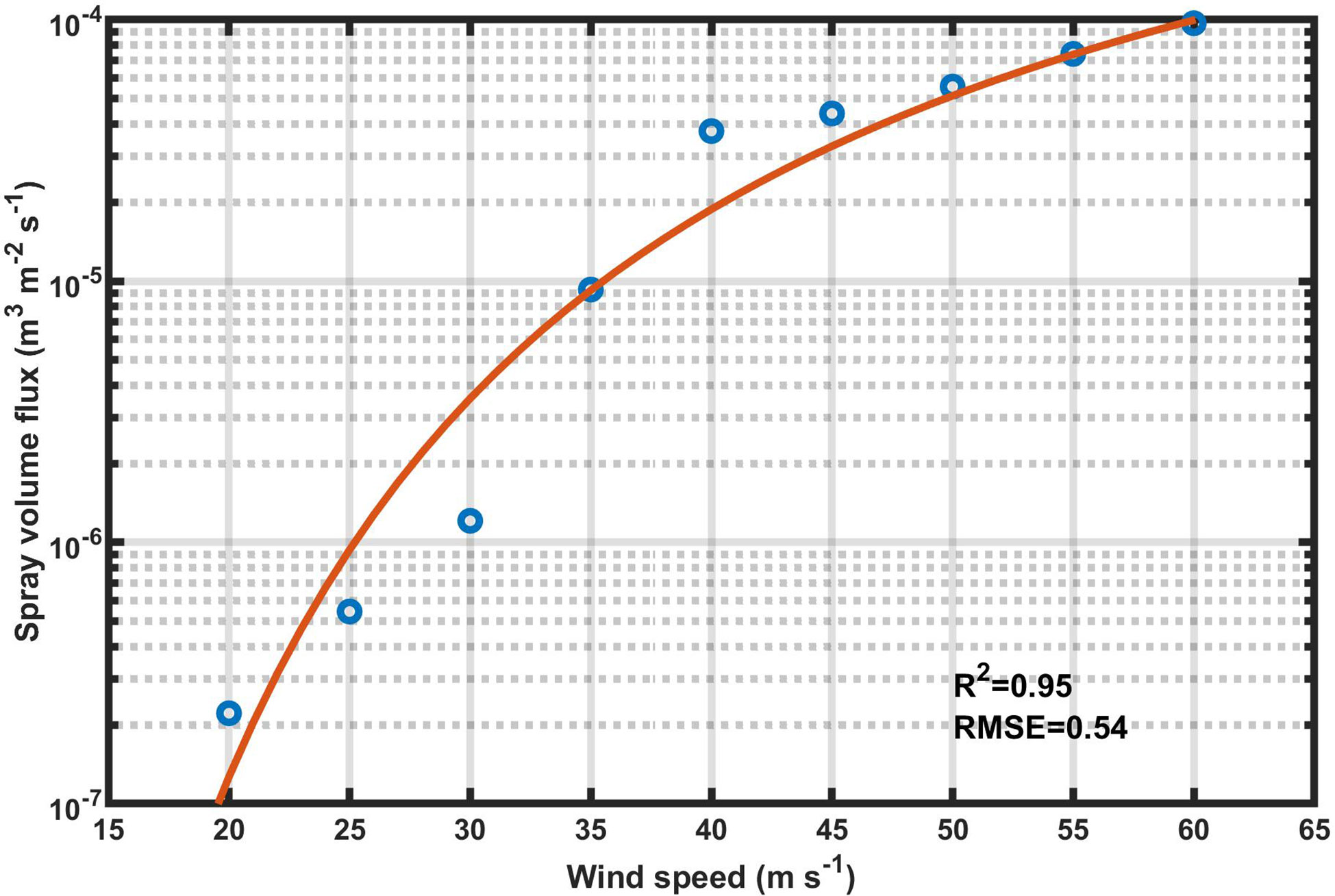
Figure 7 Spray volume flux as a function of wind speed for the laboratory observations (blue circles), and the regression (Equation 14) of spray volume flux onto wind speed (red line).

$\begin{array}{ll}\text{ln}V=-200/W-5.88& (14)\end{array}$

whose R-square statistic is 0.95. And a linear regression model between lnP and 1/W:

$\begin{array}{ll}\text{ln}P=4/W+7.13& (15)\end{array}$

whose R-square statistic is 0.86. The combination of Equations 14 and 15 then gives

$\begin{array}{ll}\text{ln}V=-50\cdot \text{ln}P+350.62& (16)\end{array}$

It is almost the same as the direct regression model between them (Equation 8), which means that the relationships we have established in the quaternary system (with wind included) for laboratory data are also self-consistent.

For both laboratory and field observations, we have established the relationship between sea spray volume flux and wind speed in the same form (Equations 11 and 15) but with different coefficients. The difference might be due to the experimental conditions which could result in different wind fetch and wave directions in the laboratory and field, as Xu et al. (2021) discussed. A uniform regression of wind speed onto spray volume needs a dimensionless parameter concerning wind speed. The relationship between wind speed and laser intensity (Equations 12 and 16) should also be influenced by the experiment parameters.

We have set up a self-consistent scheme composed of spray volume flux, laser intensity, and the environment variable. Through this approach, the estimation of sea spray volume flux from laser intensity is robust. However, the regressions in this work were done without nondimensionalization, which could limit the application of the method. That’s also why the regressions in laboratory and field experiments (Equations 13 and 14) are of different coefficients. To apply the method, Equation 9 is of importance. It sets the relationship between laser intensity and spray volume flux both for laboratory and field experiments. For another experiment with different observing laser gauges or environmental conditions, the parameters should be changed accordingly. We should also notice that the mapping of the laser intensity in the field observations on γ should be a subset of that in laboratory observations (see Figure 1B), as discussed in section 4. Besides, a regress model of wind speed on laser intensity is needed for a new experiment, so that a further relationship between wind speed and spray volume flux could be established.

Data availability statement

The original contributions presented in the study are included in the article/Supplementary Material. Further inquiries can be directed to the corresponding author.

Author contributions

GW and FQ proposed the conception of the study, AB provided the data, HM and BZ contribute to the methods and some of the figures, CH and DD performed the data analyses. All authors contributed to the article and approved the submitted version.

Funding

Special Fund of Shandong Province for Qingdao National Laboratory for Marine Science and Technology (No. 2022QNLM010102-3), the National Natural Science Foundation of China (Nos. 41821004 and 42076014), the National Program on Global Change and Air-Sea Interaction (Phase II), and the Basic Scientific Fund for National Public Research Institutes of China (No. 2021Q05).

Acknowledgments

We thank Woodside Ltd for providing the filed observations. We are grateful to Alessandro Toffoli (from the Department of Infrastructure Engineering, the University of Melbourne, Australia) for his helpful revision and suggestions on the manuscript.

Conflict of interest

The authors declare that the research was conducted in the absence of any commercial or financial relationships that could be construed as a potential conflict of interest.

Publisher’s note

All claims expressed in this article are solely those of the authors and do not necessarily represent those of their affiliated organizations, or those of the publisher, the editors and the reviewers. Any product that may be evaluated in this article, or claim that may be made by its manufacturer, is not guaranteed or endorsed by the publisher.

References

Andreas E. L. (1992). Sea Spray and the turbulent air-sea heat fluxes. J. Geophysical Res. 97, 11429–11441. doi: 10.1029/92JC00876

CrossRef Full Text | Google Scholar

Andreas E. L. (1998). A new sea spray generation function for wind speeds up to 32 m s^-1. J. Phys. Oceanography 28 (11), 2175–2184. doi: 10.1175/1520-0485(1998)028<2175:ANSSGF>2.0.CO;2

CrossRef Full Text | Google Scholar

Andreas E. L. (2002). “A review of the sea spray generation function for the open ocean,” in Atmosphere-ocean interactions, vol. 1 . Ed. Perrie W. A. (Southhampton, UK: WIT), 1–46.

Google Scholar

Andreas E. L. (2004). Spray stress revisited. J. Phys. Oceanography 34, 1429–1440. doi: 10.1175/1520-0485(2004)034<1429:SSR>2.0.CO;2

CrossRef Full Text | Google Scholar

Andreas E. L., Edson J. B., Monahan E. C., Rouault M. P., Smith S. D. (1995). The spray contribution to net evaporation from the sea: A review of recent progress. Boundary-Layer Meteorology 72 (1-2), 3–52. doi: 10.1007/BF00712389

CrossRef Full Text | Google Scholar

Anguelova M., Barber Jr R.P., Wu J. (1999). Spume drops produced by the wind tearing of wave crests. J. Phys. Oceanography 29, 1156–1165. doi: 10.1175/1520-0485(1999)029<1156:SDPBTW>2.0.CO;2

CrossRef Full Text | Google Scholar

Babanin A. V., Wake G. G., Mcconochie J. (2016). “Field observation site for air-sea interactions in tropical cyclones,” in ASME 2016 35th International Conference on Ocean, Offshore and Arctic Engineering pp. V003T02A002-V003T02A002. Am. Soc. Mech. Eng. doi: 10.1115/OMAE2016-54570

CrossRef Full Text | Google Scholar

Bao J. W., Fairall C. W., Michelson S. A., Bianco L. (2011). Parameterizations of sea-spray impact on the air-sea momentum and heat fluxes. Monthly Weather Rev. 139 (12), 3781–3797. doi: 10.1175/MWRD-11-00007.1

CrossRef Full Text | Google Scholar

Bianco L., Bao J. W., Fairall C. W., Michelson S. A. (2011). Impact of sea-spray on the atmospheric surface layer. Boundary-Layer Meteorology 140 (3), 361. doi: 10.1007/s10546-011-9617-1

CrossRef Full Text | Google Scholar

Emanuel K. A. (1995). Sensitivity of tropical cyclones to surface exchange coefficients and a revised steady-state model incorporating eye dynamics. J. Atmospheric Sci. 52, 3969–3976. doi: 10.1175/1520-0469(1995)052<3969:SOTCTS>2.0.CO;2

CrossRef Full Text | Google Scholar

Emanuel K. (2003). A similarity hypothesis for air-sea exchange at extreme wind speeds. J. Atmospheric Sci. 60 (11), 1420–1428. doi: 10.1175/1520-0469(2003)060<1420:ASHFAE>2.0.CO;2

CrossRef Full Text | Google Scholar

Fairall C. W., Kepert J. D., Holland G. J. (1994). The effect of sea spray on surface energy transports over the ocean. Global Atmosphere Ocean System 2, 121–142.

Google Scholar

Haus B. K., Jeong D., Donelan M. A., Zhang J. A., Savelyev I. (2010). Relative rates of sea-air heat transfer and frictional drag in very high winds. Geophysical Res. Lett. 37, L07802. doi: 10.1029/2009GL042206

CrossRef Full Text | Google Scholar

Iida N., Toba Y., Chaen M. (1992). A new expression for the production rate of sea water droplets on the sea surface. J. Oceanography 48 (4), 439–460. doi: 10.1007/BF02234020

CrossRef Full Text | Google Scholar

Ma H., Babanin A. V., Qiao F. (2020). Field observations of sea spray under tropical cyclone olwyn. Ocean Dynamics 70, 1439–1448. doi: 10.1007/s10236-020-01408-x

CrossRef Full Text | Google Scholar

Melville K. W., Matusov P. (2002). Distribution of breaking waves at the ocean surface. Nature 417, 58–63. doi: 10.1038/417058a

CrossRef Full Text | Google Scholar

Monahan E. C., Spiel D. E., Davidson K. L. (1986). “A model of marine aerosol generation via whitecaps and wave disruption,” in Oceanic whitecaps(Dordrech:Springer), 167–174. doi: 10.1007/978-94-009-4668-2_16

CrossRef Full Text | Google Scholar

O’Dowd C. D., de Leeuw G. (2007). Marine aerosol production: A review of the current knowledge. Philos. Trans. R. Soc. A365, 1753–1774. doi: 10.1098/rsta.2007.2043

CrossRef Full Text | Google Scholar

Shi R., Xu F. (2022). An improved parameterization of sea spray-mediated heat flux using Gaussian quadrature: Case studies with a coupled CFFv2.0-WW3 system. Geoscientific Model. Dev. Discussions. [preprint]. Available at: https://gmd.copernicus.org/preprints/gmd-2022-233 (Accessed December 30, 2022).

Google Scholar

Soloviev A. V., Lukas R., Donelan M. A., Haus B. K., Ginis I. (2014). The air-sea interface and surface stress under tropical cyclones. Sci. Rep. 4, 5306. doi: 10.1038/srep05306

CrossRef Full Text | Google Scholar

Takagaki N., Komori S., Suzuki N., Iwano K., Kurose R. (2016). ). mechanism of drag coefficient saturation at strong wind speeds. Geophysical Res. Lett. 43 (18), 9829–9835. doi: 10.1002/2016GL070666

CrossRef Full Text | Google Scholar

Toffoli A., Babanin A. V., Donelan M., Haus B., Jeong D. (2011). Estimating sea spray volume with a laser altimeter. J. Atmospheric Oceanic Technol. 28, 1177–1184. doi: 10.1175/2011jtech827.1

CrossRef Full Text | Google Scholar

Troitskaya Y., Kandaurov A., Ermakova O., Kozlov D., Sergeev D., Zilitinkevich S. (2018). The “bag breakup” spume droplet generation mechanism at high winds. part I: spray generation function. J. Phys. Oceanography 48 (9), 2167–2188. doi: 10.1175/JPO-D-17-0104.1

CrossRef Full Text | Google Scholar

Veron F. (2015). Ocean spray. Annu. Rev. Of Fluid Mechanics 47, 507–538. doi: 10.1146/annurev-fluid-010814-014651

CrossRef Full Text | Google Scholar

Wojtanowski J., Zygmunt M., Kaszczuk M., Mierczyk Z., Muzal M. (2014). Comparison of 905 nm and 1550 nm semiconductor laser rangefinders’ performance deterioration due to adverse environmental conditions. Opto-Electronics Rev. 22 (3), 183–190. doi: 10.2478/s11772-014-0190-2R

CrossRef Full Text | Google Scholar

Xu X., Voermans J. J., Ma H., Guan C., Babanin A. V. (2021). A wind-wave-dependent sea spray volume flux model based on field experiments. J. Mar. Sci. Eng. 9, 1168. doi: 10.3390/jmse9111168

CrossRef Full Text | Google Scholar

Zhao B., Qiao F., Cavaleri L., Wang G., Bertotti L., Liu L. (2017). Sensitivity of typhoon modeling to surface waves and rainfall. J. Geophysical Research-Oceans 122 (3), 1702–1723. doi: 10.1002/2016JC012262

CrossRef Full Text | Google Scholar

Zhao D., Toba Y., Sugioka K. I., Komori S. (2006). New sea spray generation function for spume droplets. J. Geophysical Research-Oceans 111 (C2), C02007. doi: 10.1029/2005JC002960

CrossRef Full Text | Google Scholar