
94% of researchers rate our articles as excellent or good
Learn more about the work of our research integrity team to safeguard the quality of each article we publish.
Find out more
ORIGINAL RESEARCH article
Front. Mar. Sci., 22 December 2022
Sec. Coastal Ocean Processes
Volume 9 - 2022 | https://doi.org/10.3389/fmars.2022.1100510
This article is part of the Research TopicMacroecology of Coastal Zone under Global ChangesView all 15 articles
 Ying-Ying Chen1
 Kai Yu2,3,4*
The eastern equatorial Pacific exhibits a pronounced westward propagating sea surface temperature annual cycle (SSTAC). The responses of the equatorial Pacific SSTAC to CO2-induced global warming are examined using 15 Coupled Model Intercomparison Project Phase 5 (CMIP5) experiments. The annual cycle patterns of global-warming simulations over 2006-2100 are compared with that of present-day simulations over 1850-2005. We see no statistically significant changes in SSTAC amplitude in the future. A coupled dynamical diagnostic framework is adopted to assess four factors, including the damping rate, phase speed and strength of the annual and semi-annual harmonic forcing of SSTAC. Under global warming, changes relative to the present-day simulations in these four diagnostic factors have a clear multi-model trend. Most coupled models exhibit relatively weaker (an average of 18%) propagation speed, and stronger annual (18%) and semi-annual (39%) external forcing. Half of the models show a relatively stronger (about one time) damping rate, while the rest show a weaker (30%) damping rate. When these four diagnostic factors are further condensed into a dynamical response factor and a forcing factor, it is revealed that the same annual cycle amplitudes with respect to the present-day simulations may result from the compensations in terms of bias in the dynamical response factor and forcing factor under increased CO2-induced warm climate.
Sea surface temperature (SST) in the eastern tropical Pacific cold tongue region exhibits a pronounced annual cycle, with a warm phase during boreal spring and a cold phase during fall, although the sun moves across the equator twice yearly (Wyrtki and Meyers, 1976; Horel, 1982; Mitchell and Wallace, 1992; Wang, 1994; Xie, 1994). The main cause for the generation of this SST annual cycle (SSTAC) is the hemispheric asymmetries of the tropical Pacific climatological mean conditions (Mitchell and Wallace, 1992; Xie, 1994). These asymmetries are caused by the distribution of continents and maintained by coupled ocean-atmosphere interaction (Philander et al., 1996; Xie, 2004). In the eastern Pacific, the northern position of the intertropical convergence zone (ITCZ) (e.g., Hanson et al., 1967; Manabe et al., 1974; Philander and Seigel, 1985; Xie and Philander, 1994) maintains the southeast trade winds across the equator year-round with annually varying intensity. This annually-varying cross-equatorial wind brings the off-equatorial annual insolation onto the equator and remotely forces a westward propagating SSTAC at the equator by controlling the strength of cold-water upwelling, wind-driven evaporation and the amount of the stratus clouds via ocean-atmosphere interactions (Chen and Jin, 2018; Wengel et al., 2018). SSTAC in the eastern equatorial Pacific arises from the hemispheric asymmetries of the climate mean states and is amplified by coupled tropical ocean-atmosphere interactions. The tropical SSTAC interacts with ENSO (e.g., Tziperman et al., 1994; Jin et al., 1994; Chang and Philander, 1994; Jin, 1996; Stuecker et al., 2013; Stuecker et al., 2015), as well as with anthropogenic greenhouse warming. The increasing concentrations of the greenhouse gases, such as CO2, are the main cause of the acceleration of global warming. The increasing ocean temperatures will have substantial effects on marine ecosystems (Doney et al., 2012; Hollowed et al., 2013; Brander, 2013). Ocean temperature modulates physiological processes in all marine organisms (Rivkin and Legendre, 2001; Drinkwater et al., 2010; Ottersen et al., 2010; Deutsch et al., 2015). SST, as an important driver of marine ecosystem, is dominated by the seasonal variability in the tropical coastal regions. The cross-equatorial wind forces coastal upwelling and brings subsurface cold water and nutrients to the surface, resulting in a high production in the eastern boundary of the Pacific Ocean.
Future climate projection is mostly based on climate model simulations. Under greenhouse warming, many climate models have projected a significant change in the SSTAC from low to high latitudes (Timmermann et al., 2004; Biasutti and Sobel, 2009; Xie et al., 2010; Sobel and Camargo, 2011; Stine and Huybers, 2012; Dwyer et al., 2012; Carton et al., 2015; Liu et al., 2017; Alexander et al., 2018; Liu et al., 2020). In particular, models display a great diversity of equatorial Pacific SST changes, including the east-west gradient of the annual mean SST (Liu et al., 2005; Collins and Modeling Groups, 2005; DiNezio et al., 2009) and SSTAC (Timmermann et al., 2004; Xie et al., 2010; Sobel and Camargo, 2011) in response to global warming. Timmermann et al. (2004) simulated a strong intensification of the SSTAC in the eastern equatorial Pacific in response to greenhouse warming in a coupled general circulation model. They illustrated that the tropical Pacific mean climate changes due to greenhouse warming provide seeding for the anomalous SSTAC and the tropical ocean-atmosphere interactions lead to amplification. Xie et al. (2010) showed a pronounced annual cycle in the equatorial Pacific under greenhouse warming in a climate model. They pointed out that the upwelling damping mechanism (Clement et al., 1996; Cane et al., 1997) dominates the equatorial Pacific annual cycle in SST warming. Sobel and Camargo (2011) studied 24 Coupled Model Intercomparison Project Phase 3 (CMIP3) models and analyzed changes in the tropical SST under greenhouse warming. They found that the SST annual mean warming, with a local maximum in the equatorial Pacific, is greater in the Northern Hemisphere than in the Southern Hemisphere and the SST seasonal change is a warming in the summer hemisphere and cooling in the winter hemisphere, inducing an enhanced seasonal cycle in the mid-latitudes. They attributed these SST change patterns to thermodynamic consequences of surface trade winds, which increase in the winter hemisphere and decrease in the summer hemisphere. However, they did not address the seasonal cycle on the equator in detail.
In summary, tropical patterns of SSTAC under global warming and relevant physical processes are still not systematically studied as has been the global annual mean warming. SSTAC can be caused by several factors, such as mean circulation advection, zonal advection, Ekman pumping feedback, thermocline feedback and thermodynamic feedback (Jin et al., 2006; Chen and Jin, 2018). The various relative importance of these feedbacks among models induces diverse properties of SSTAC and its uncertainties. To discern and separate the possible factors, Chen and Jin (2017; 2018) proposed a coupled dynamic diagnostics framework to analyze the equatorial Pacific SSTAC in terms of damping rate, propagation speed, external annual and semi-annual forcing and apply it to explore the diversities of the SSTACs in CMIP5 simulations. To illustrate the changes of the equatorial Pacific SSTAC in response to global warming, we describe its major patterns in global warming simulations of the CMIP5 models and use this framework to systematically analyze the dynamics and inter-model diversities of these SSTACs in this study.
The remainder of this paper is structured as follows. Section 2 describes the coupled models and observational datasets and introduces the coupled dynamic diagnostics framework of SSTAC. Section 3 presents the features of equatorial Pacific SSTAC change response to global warming based on CMIP5 simulations. Section 4 describes the dynamical diagnostic results of SSTAC change. In section 5, we examine the dynamic and forcing controls of SSTAC change and discuss the possible reasons for the diversities of SSTAC change. In section 6, we give a summary and discussion.
In this study, we analyze 15 model simulations from the CMIP5 coupled general circulation models (CGCMs) (Table 1). Representative concentration pathway 4.5 (RCP4.5) is a high greenhouse gas emission scenario that reaches a radiative forcing level of 4.5 W/m2 by the year 2100 (Taylor et al., 2011). RCP4.5 simulations over 2006-2100 represent the global-warming climate. Historical simulations, which cover the period 1850-2005, represent the present-day climate. We select these 15 models from which all variables required for dynamical diagnoses of the annual cycle of the surface layer (constant 25 m in this study), including monthly mean SST, ocean current, surface meridional wind, shortwave/longwave radiation, latent heat flux, and sensible heat flux, are available in the eastern equatorial Pacific. All model outputs are interpolated from the native model grid onto the same uniform 1°×1° horizontal grid prior to any diagnostic computation. The ‘observed’ SST, current velocity, surface wind and surface heat flux components are taken from the monthly ERA40 atmospheric reanalysis (Uppala et al., 2005) on a 2.5°×2.5° horizontal grid and the monthly ORA-S3 (Balmaseda et al., 2008) of ocean analysis system produced at ECMWF on a 1°×1° horizontal grid, from 1959 to 2001.
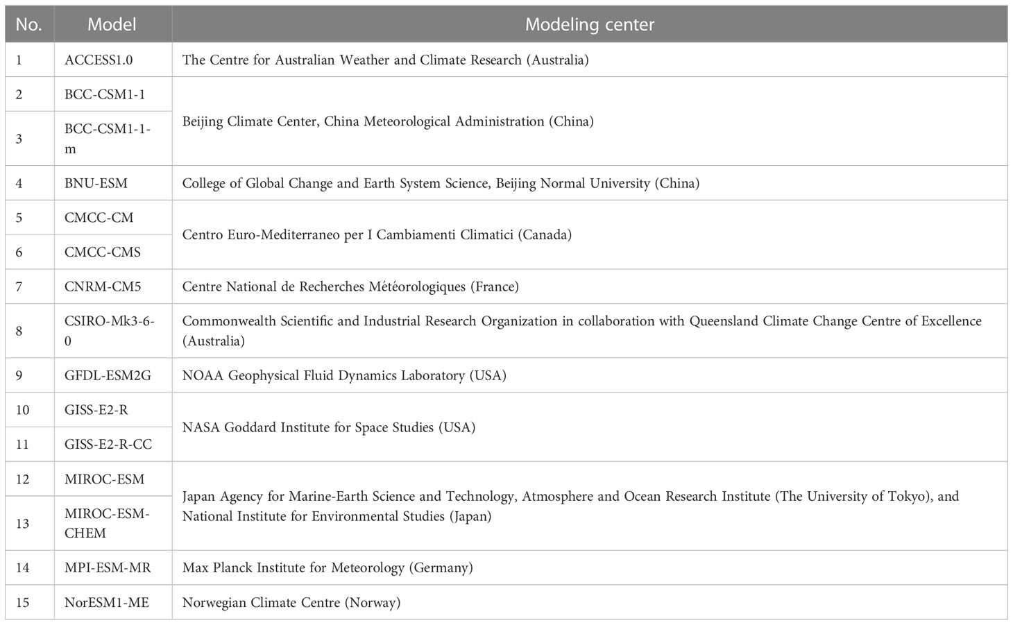
Table 1 List of the CMIP5 models used in this study.
Following Chen and Jin (2017; 2018), we establish an approximate coupled dynamic diagnostics framework for understanding the nature of the annual cycle in the equatorial Pacific cold tongue region. This framework utilizes a heat budget equation for SSTAC, which can be written as follows.
where
Here, all variables with an overbar denote the annual mean climate state. The variables T, u, v and Q denote the annual cycles of SST, horizontal surface currents and net surface heat flux, respectively. Po is the density of seawater, Cp is the heat capacity, h is specified as the depth of the surface layer, NL is the nonlinear term, and Res is the residual. The vertical entrainment is defined as we∂T/∂z=we(T−Tsub)/h , where Tsub and we=h·Δv are the subsurface temperature and vertical entrainment velocity at the base of the mixed layer. M(x) is a Heaviside function where M(x)=0, if x<0, and M(x)=x, otherwise. We regroup the SST heat budget into seven terms as in the ENSO heat budget analysis (An et al., 1999; Jin et al., 2006; Chen and Jin, 2018). The right hand of Eq. (1) represents, from left to right, the mean circulation term (MC), the zonal advection term (ZA), the Ekman pumping term (EK), the thermocline effect term (TH), the thermodynamic term (TD), the nonlinear term (NL), and the residual term (res), respectively.
We adopt four main assumptions to develop a simple coupled framework for the equatorial SSTAC as described in Chen and Jin (2017; 2018): (1) the decomposition of the equatorial annually varying wind into a coupled part as the direct response to the annual equatorial SST and an external part serving as external forcing; (2) the quasi-equilibrium approximation of oceanic dynamic response to the equatorial annual wind forcing or so-called fast-wave limit as termed in Jin and Neelin (1993); (3) the decomposition of the thermodynamic heating into a coupled part related directly to the equatorial annual SST and an external part serving as forcing; and (4) the assumption that the linear compounding coupled operator of the SST derived under assumptions (1-3) can be further approximated by a linear damping and a zonal propagation term. It should be noted that because we have adopted the fast-wave limit approximation to assume that annual variations in ocean current, upwelling and thermocline are in quasi-equilibrium with the annual wind stress, the coupled framework does not involve the ocean memory residing in adjustment through the ocean wave dynamics. Thus, the coupled framework could be considered equivalent to the SST-mode framework described in Neelin (1991) and Jin and Neelin (1993), except here, we also consider the external annual forcing.
With these assumptions, we may approximately define the equatorial SST in the following equation:
Here, ω=2π/1yr, φ is the relative phase of the annual forcing to the semi-annual forcing, R is the remainder. In this simple form, SSTAC is expressed by four factors (λ, c, f1, f2), which are the damping rate, westward phase speed, annual and semi-annual forcing amplitudes, respectively. More details can be found in Chen and Jin (2017; 2018). These four factors (λ, c, f1, f2) are estimated using least-squares regressions. By turning the heat budget equation (1) into an approximate coupled and forced linear model in the form of Eq. (8), we can describe SSTAC in terms of the four factors mentioned above. Sections 3-5 demonstrate how this simplification may offer insights into the response of the equatorial Pacific SSTAC to global warming in simulations.
To illustrate the change in simulated SSTAC of the equatorial Pacific under global warming, we plot and contrast the equatorial (5°S-5°N) SST annual evolutions in the eastern Pacific (150-90°W). Figures 1A, B show the observation and the multi-model ensemble mean (MME) SSTAC of the present-day simulations. The observed equatorial SST in the cold tongue region shows a strong westward propagation. This annual cycle reaches its warm peak at 1.5°C during March and April, while cold peak at -1.0°C during August and October. Its amplitude, defined as half the peak-to-peak range, is largest at about 1.25°C and mainly confined to the cold tongue region between 110 and 80°W. Compared to the observation, the MME of the present-day simulated SSTAC shows a weaker amplitude of 1°C and is displaced westward. The warm phase arrives 1 month later than that in observation. Although the timing of the cold phase in August is represented successfully, it decays more rapidly.
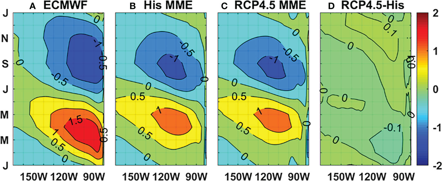
Figure 1 Time-longitude plots of SSTAC (°C) averaged between 5°S and 5°N in the eastern equatorial Pacific based on (A) ECMWF reanalysis dataset, and MME of (B) the historical and (C) RCP4.5 simulations, and (D) their difference (contour interval = 0.5°C).
In the present-day simulations, the models show a range of spatial and temporal patterns of the equatorial SSTAC, as shown in Figure 2. Most of the models roughly capture the major features of SSTAC, while a few of them (e.g., BCC-CSM1-1, BCC-CSM1-1-m) have their simulated annual cycle whose behavior to a large extent is dominated by the semi-annual component. Under enhanced CO2 conditions, The MME of the global-warming simulations is almost the same as that of the present-day simulations (Figures 1C, D).
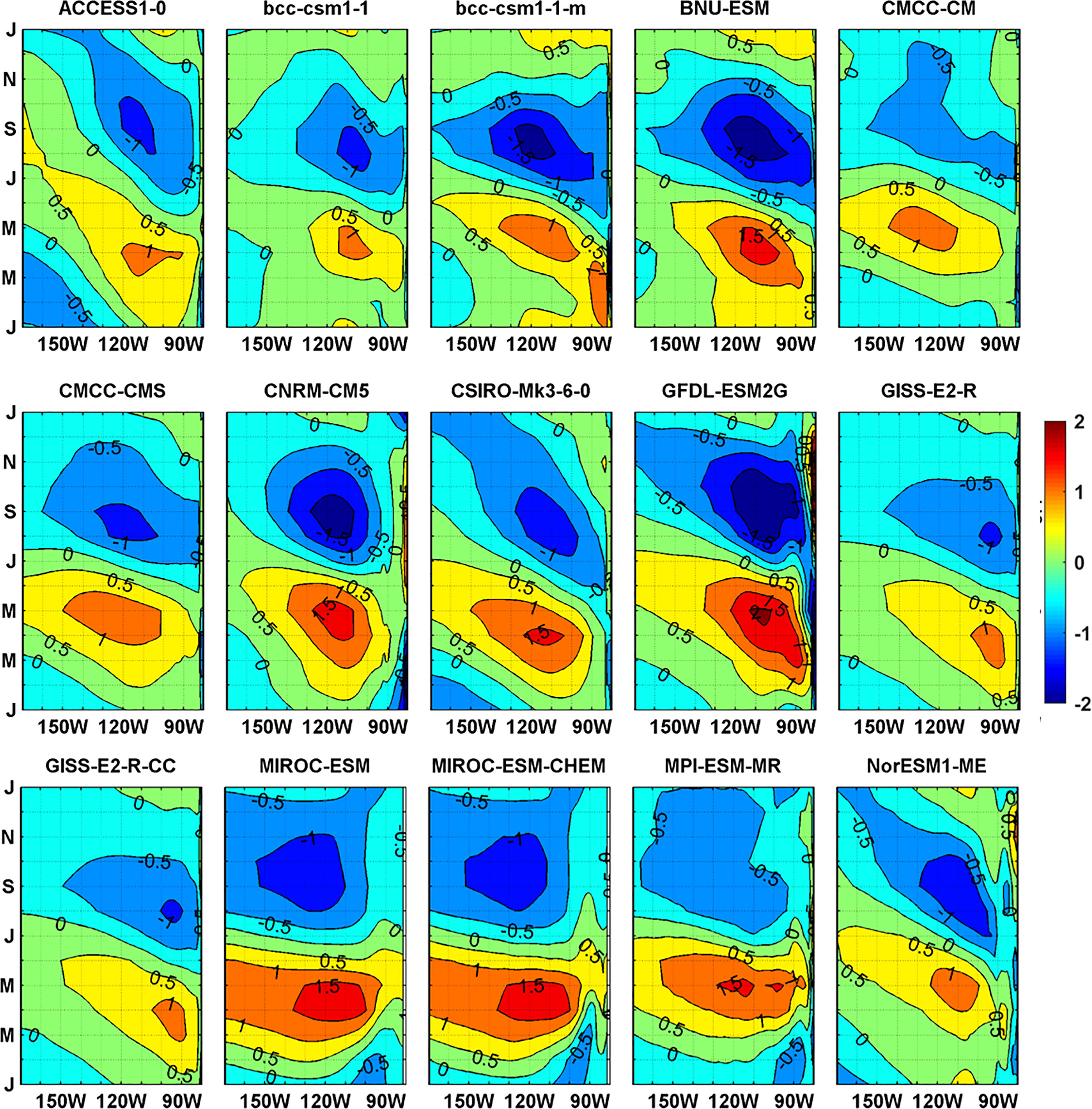
Figure 2 Same as Figure 1B, but for the individual 15 models in the historical period.
Compared with the present-day simulations, most models show a slight change in the equatorial SSTAC patterns under global warming (Figure 3). The ACCESS1-0, CNRM-CM5 and NorESM1-ME models are exceptions, with a weakening of the annual cycle, which has colder SSTs during spring and warmer SSTs during fall. It is worth noting that compared to the present-day scenario, although MIROC-ESM and MIROC-ESM-CHEM have enhanced amplitudes in the region between 110 and 90°W where it shows a semi-annual cycle, their amplitudes have no obvious change between 150 and 110°W where it shows a pronounced annual cycle under global warming. Both of their simulated equatorial SSTACs in the present-day and global warming climates are displaced more westward between 150 and 100°W compared with the observation.
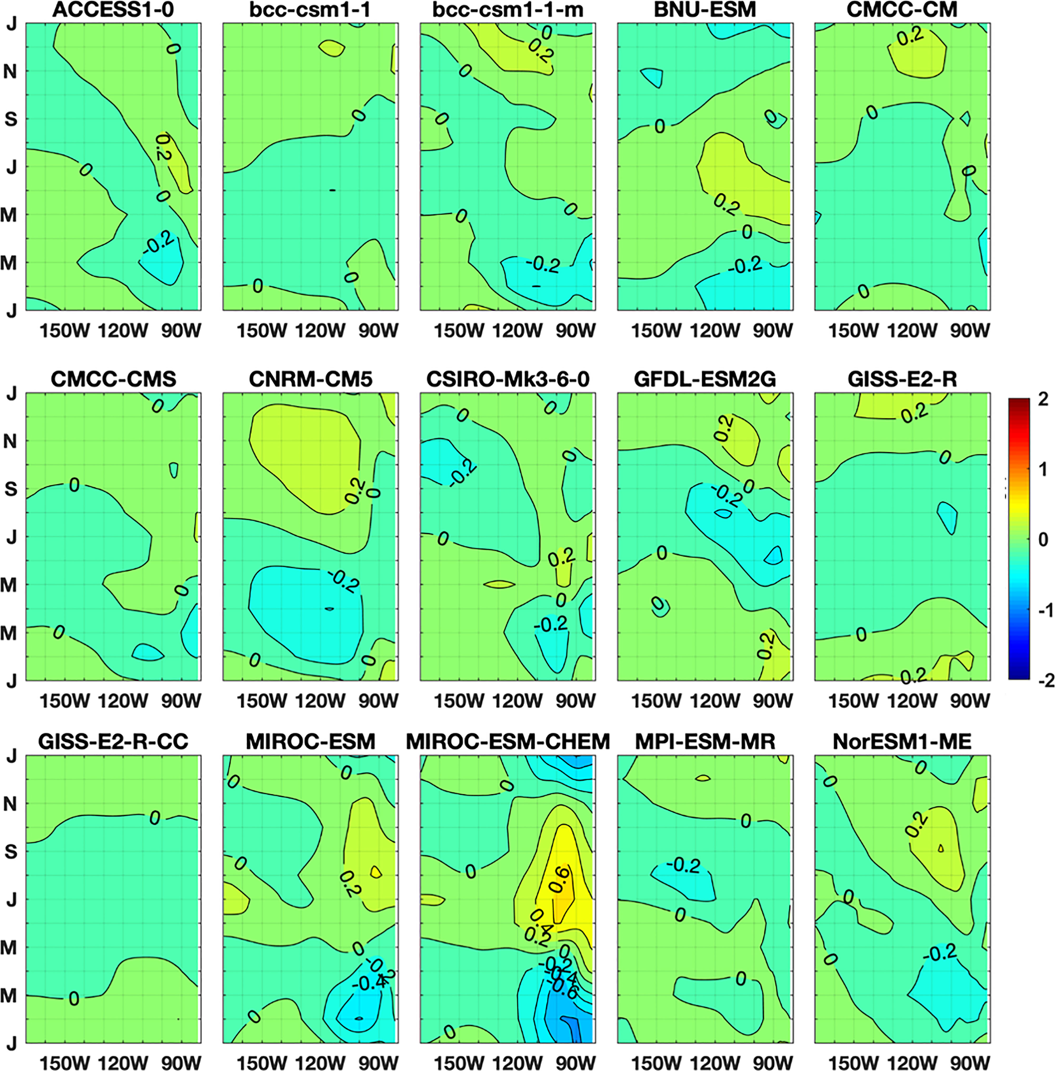
Figure 3 Same as Figure 1D, but for the difference between historical and RCP4.5 (where the difference is calculated as RCP4.5 minus historical).
We calculate the zonal averages of SSTAC amplitude over the main domain, which is defined by the amplitude being higher than the average of the entire domain (170-80°W). Figure 4A shows that under enhanced CO2 conditions, the MME amplitude of SSTAC (A) in the eastern equatorial pacific region has almost the same magnitude as that in the present-day. However, nearly all (13 of 15) models underestimate the amplitudes of the annual cycle in these two climates compared to observations. In fact, it is not clear whether the SSTAC is stronger in the projections on a future climate change compared to the present-day simulations, as 4 of 15 models (ACCESS1-0, BNU-ESM, CNRM-CM5 and NorESM1-ME) show weakened SSTAC amplitudes, 4 of 15 models (GFDL-ESM2G, GISS-E2-R, GISS-E2-R-CC and MPI-ESM-MR) show increased SSTAC amplitudes and the remaining 7 of 15 models show no change. Figures 4B, C show the amplitudes of annual (A1) and semi-annual (A2) harmonic component of observed and simulated SSTAC, respectively. The annual harmonic component has a similar trend of total amplitude and is compensated by the semi-annual harmonic component (e.g., BCC-CSM1-1-m), which shows a systematic trend toward an increase under a warmer climate. Both the MME of total amplitude (A) of the present-day and global warming climates are about 15% lower than the observed, and their annual components (A1) are about 23% and 27% lower than the observed, respectively, whereas their semi-annual components (A2) are about 20% and 32% higher.
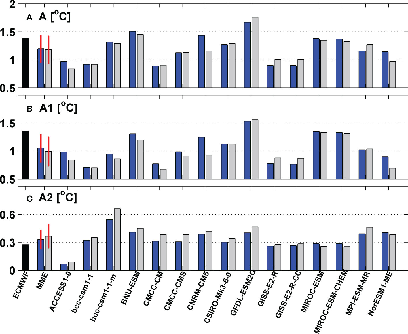
Figure 4 The amplitude (°C) of (A) SSTAC, and its (B) annual and (C) semi-annual components based on ECMWF reanalysis dataset (black bars), MME and each of 15 models in the historical period (blue bars) and RCP4.5 scenario (grey bars).Red lines represent the inter-model standard deviation.
In summary, compared to the present-day scenario, most models have roughly equivalent SSTAC strengths in the eastern equatorial Pacific, with a slightly reduced annual component and consistently increased semi-annual component under RCP4.5. In the next section, we further identify the contributions to the diverse magnitudes of change from model to model by employing the dynamical diagnostic framework (section 2).
To investigate the causes of change in SSTAC in response to global warming, this section uses the dynamical diagnostic framework formulated in Section 2 to explore the physical mechanisms. This framework may approximately describe the equatorial annual cycle by four factors (λ, c, f1, f2), in terms of the damping rate, westward propagation speed, annual and semi-annual external forcing, respectively.
These four factors are estimated for the 15 couple models in the present-day and global warming climate, as shown in Figure 5. Here for the damping rate and westward propagation speed, we estimate the zonal averages over the main domain. For the annual and semi-annual external forcing, we calculate the averages over the eastmost 70% of the main domain., the zonal averages of (λ, c, f1, f2) of the observed SSTAC are (-0.4 month-1, 0.58 m s-1, 0.61°C month-1, 0.13°C month-1). There are wide ranges of these four factors among coupled models. The zonal average MMEs of (λ, c, f1, f2) are (-0.25 month-1, 0.56 m s-1, 0.42°C month-1, 0.19°C month-1) and (-0.26 month-1, 0.46 m s-1, 0.49°C month-1, 0.26°C month-1) for present-day and global-warming climate, respectively. The results indicate that compared with observations, most models of two climate periods produce lower annual external forcing and damping rate and higher semi-annual external forcing, but comparable propagation speed. The results also show that in a majority of models, the annual and semi-annual external forcing increase from the present-day to global warming simulations, while the propagation speed decrease. It should be noted that under warming climate, the increase of the semi-annual forcing, close to 39%, is larger than the annual forcing (18%). Although the MME of the damping rate does not change much, the inter-model differences in its change are substantial.
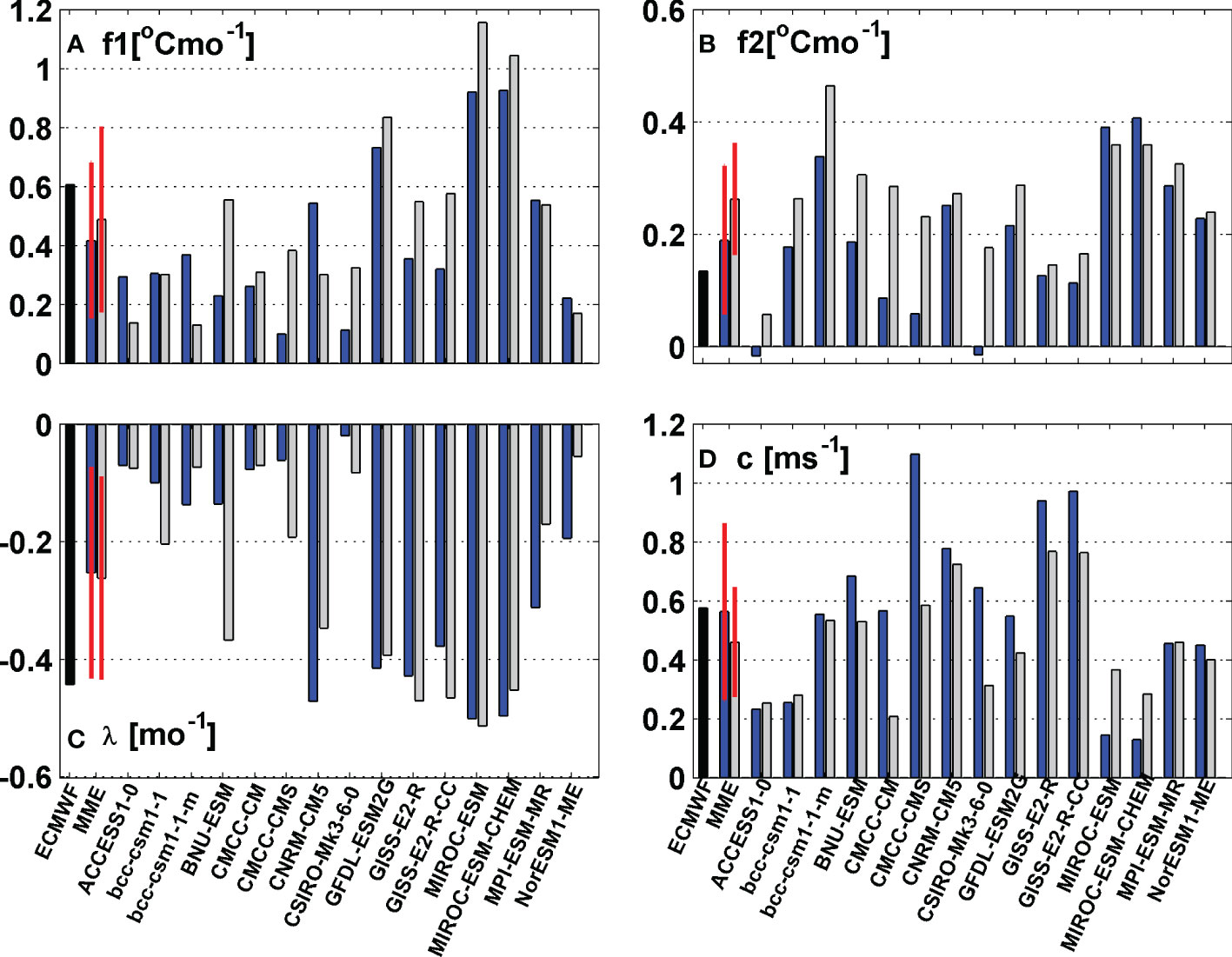
Figure 5 (A) Annual and (B) semi-annual external forcing (°C month-1), (C) the damping rate (month-1) and (D) the westward propagation speed (m/s) based on ECMWF reanalysis dataset (black bars), MME and each of 15 models in the historical period (blue bars) and RCP4.5 scenario (grey bars). Red lines represent the inter-model standard deviation.
Moreover, further detailed analysis of changes of (λ, c, f1, f2) and the respective components of the different feedback terms in Eq. (1) in these four factors under enhanced CO2 conditions is performed in Figure 6. The result shows how the MMEs of these four factors change under a warmer climate and their contributions from the mean circulation, the zonal advection, the Ekman pumping feedback, the thermocline feedback, the thermodynamic feedback, the nonlinear effect and the residual.
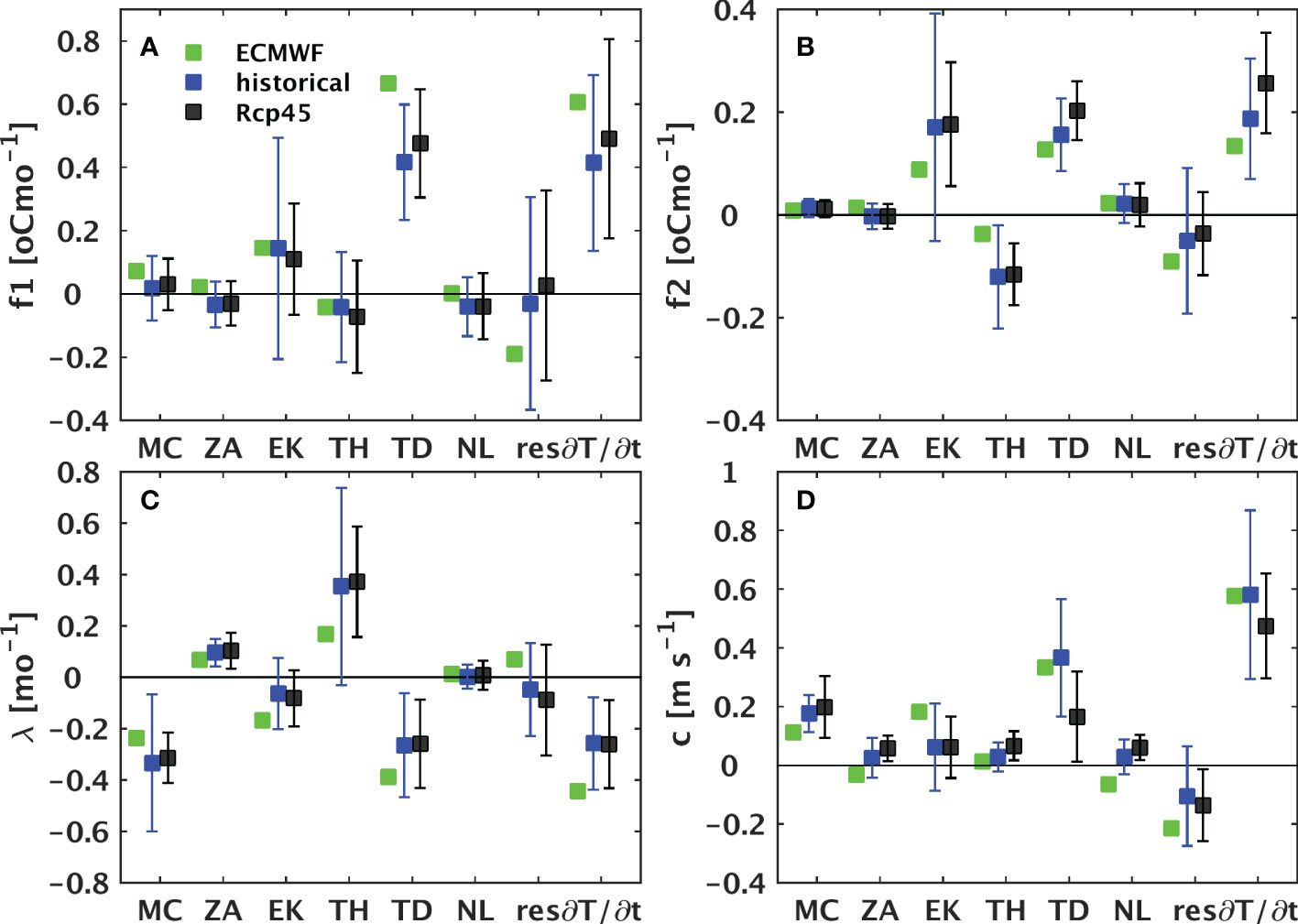
Figure 6 Diagrams for total and individual contribution from the different feedback terms (MC, ZA, EK, TH, TD, NL and Res) of the SST tendency (Tt) to (A) the annual and (B) semi-annual harmonic external forcing (ºC month-1), (C) the damping rate (month-1) and (D) the westward propagation speed (m s-1) based on the ECMWF reanalysis dataset (green squares), MME in the historical period (blue squares) and RCP4.5 scenario (black squares). Whiskers represent the inter-model standard deviation.
Under a warmer climate, compared to the observation, the weak annual forcing is mainly due to the weakening of the contribution from the thermodynamic term, and there is some cancelation by the residual term, which might be the effect of sub-grid processes (Figure 6A). The increase of the semi-annual forcing derived from the Ekman pumping and thermodynamic terms are the two main positive contributors to the increase of the total semi-annual forcing. The decrease of the semi-annual forcing derived from the thermocline effect term is the main negative contributor, which tends to reduce the overall increase of the semi-annual forcing in response to global warming (Figure 6B). There is a stronger positive growth rate in the thermocline effect term and a weaker negative growth rate in the damping rate from the thermodynamic term. Both of them give rise to lower damping of the annual cycle. Although the damping rate derived from the mean circulation and residual terms are slightly stronger negative, they are still insufficient to encounter the two contributors above. As a result, the SSTAC has a lower damping rate than the observation in response to a warmer climate (Figure 6C). There is a notable weakening of propagation speed from the thermodynamic and Ekman pumping terms, which are partly canceled by the nonlinear and residual terms. This leads to a slightly weak westward propagation (Figure 6D). Figure 6 also clearly shows that the thermodynamic term is the key source of the increase of the annual and semi-annual external forcing and the decrease of the propagation speed from the present-day to global warming simulations.
Since the dominant contribution from the thermodynamic term (TD), we further decompose it into its four components of short-wave (SW), long-wave (LW), latent (LH) and sensible (SH) heat flux. As shown in Figure 7, TD, SW and LH all have substantial changes among different climates, suggesting that various behaviors of thermodynamics are attributable to the diversity of the response of the short wave radiation and latent heat flux to anomalous forcing (e.g., enhanced CO2 conditions).
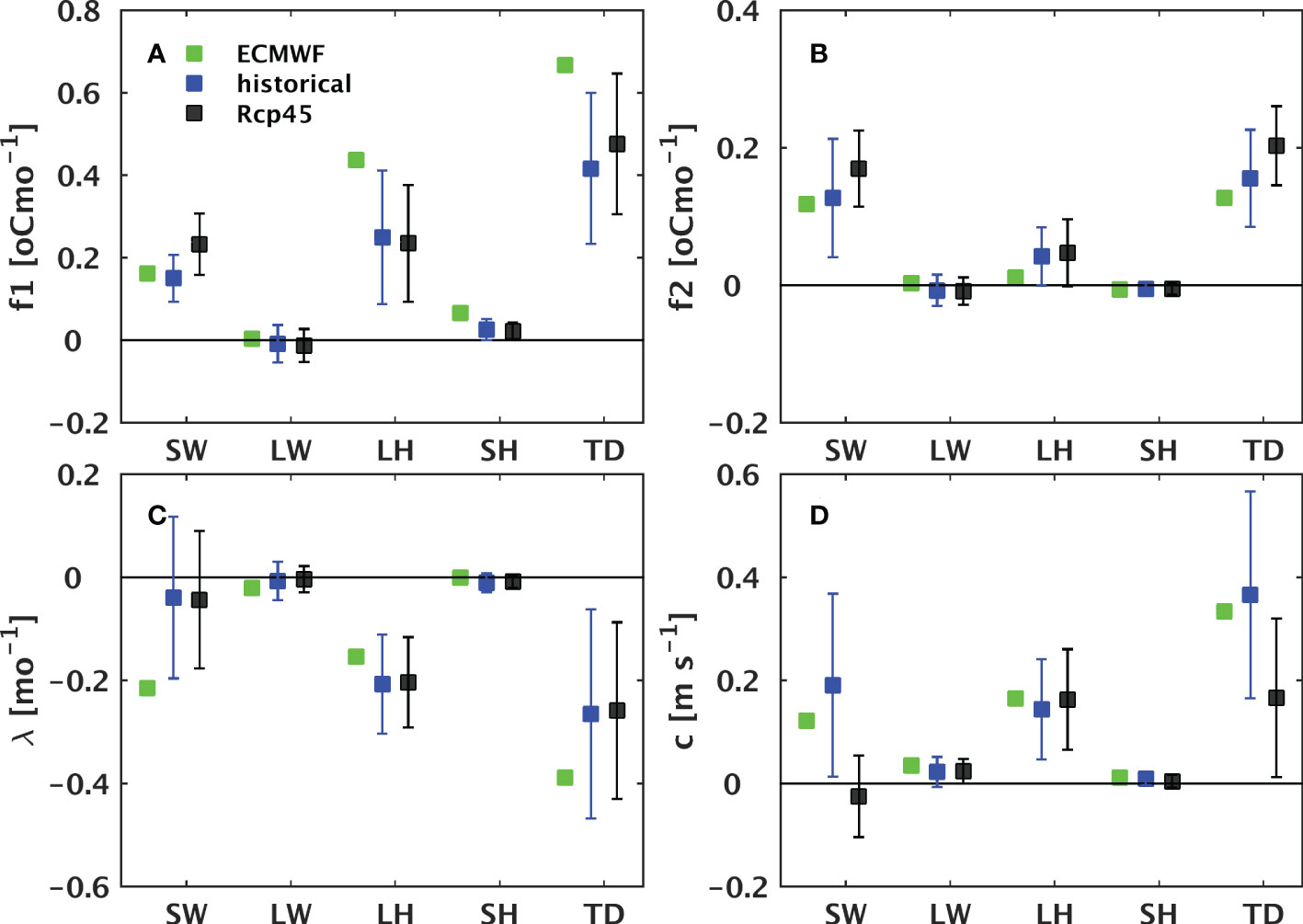
Figure 7 Same as Figure 6, but for contributions from the thermodynamic (TD) process and its components, the SW, LW, LH and SH. Whiskers represent the inter-model standard deviation.
The main contributor to the differences between the two climate periods and between the observation and models is the short-wave radiation, as can be inferred from Figure 7. As an exception, the differences in the annual forcing may be primarily attributed to the latent heat flux. Under a warmer climate, compared to observation, the decreased annual forcing (increased semi-annual forcing) may be largely attributed to the weakened annual forcing (strengthened semi-annual forcing) from the LH as a result of decreased annual forcing (increased semi-annual forcing) from thermodynamics.
The above discussion shows that the SSTAC in the Pacific cold tongue region is mainly controlled by the internal dynamic factors, namely the damping rate λ and westward propagation speed c, and the external forcing factors that depend on the annual harmonic f1 and semi-annual harmonic f2 forcing. Under a warmer climate, despite the small change in the SSTAC amplitude (A), the changes in the internal dynamics and external forcing as measured by (λ, c, f1, f2) are remarkable and have great inter-model spreads. In this section, we propose a theory for better understanding the impact of climate change on the SSTAC. To further examine the effect of the internal dynamics and forcing on the SSTAC amplitude change under increased CO2 conditions, we combine the two internal dynamical factors of the damping rate and propagation speed into a single dynamical response factor. Here we briefly define and describe the dynamical response factor (refer to Chen and Jin, 2017; Chen and Jin, 2018 for a detailed explanation). The dynamical response factor can be driven using the temporal and volume averaged form of the linearized SST perturbation equation (8) that is based on several approximations as follows:
In the above, denotes the temporal average quantities, 〈B〉 the volume average quantities over the zonal domain region. We solve the dynamical response factor D by using the individual longitudinally varying factors (λ, c, f1, f2) estimated from the CMIP5 models of two climate periods and observation shown in Figure 5. Figure 8 shows scatterplots of the SSTAC amplitudes A versus the total external forcing that includes the annual and semi-annual harmonic components multiplied by the dynamical response factor f·D. The SSTAC amplitude and the combination of the external forcing with the dynamical response factor are highly correlated at 0.81 and statistically significant at 99% confidence level. Due to this good correlation, f·D may be considered a simplified measurement of the SSTAC amplitude in the observation and coupled models. In other words, changes in SSTAC properties in coupled models under a warmer climate scenario can be attributed to the changes in the external forcing factor and dynamical response factor.
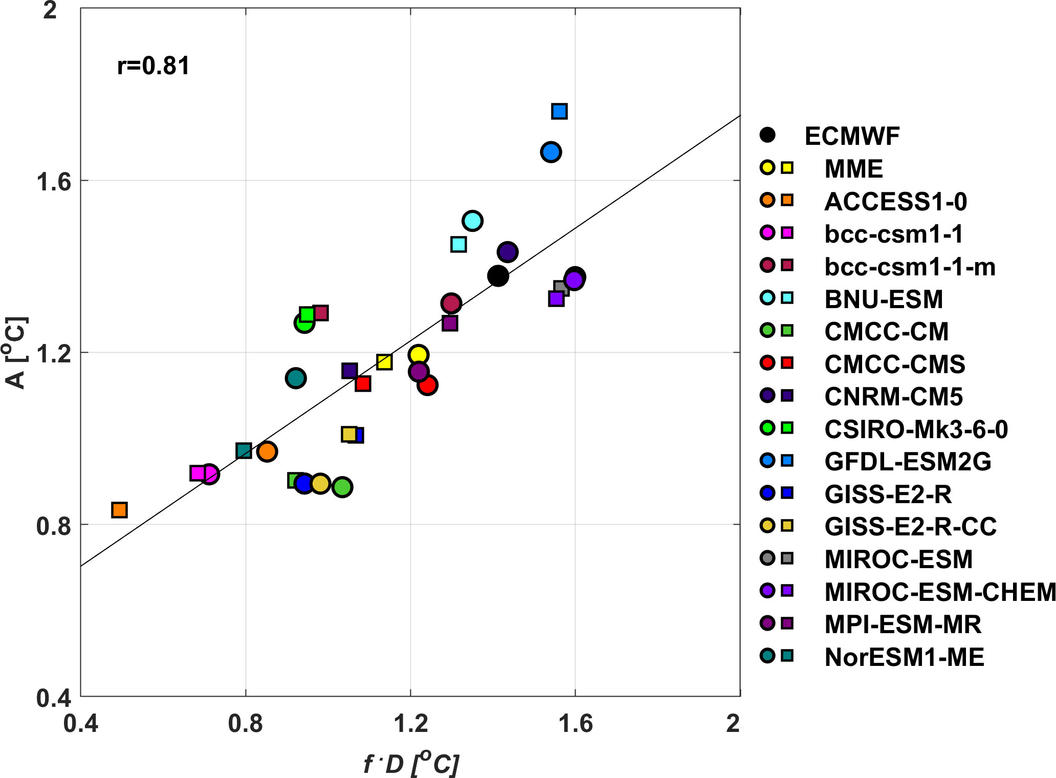
Figure 8 Amplitudes of SSTAC related to the total external forcing f, which includes the annual and semi-annual components, multiplied by the dynamical response factor D, based on ECMWF reanalysis dataset (black circle), MME and each of 15 models in the historical period (colored circles) and RCP4.5 scenario (colored squares).
To contrast the dependence of A on f and D, the different SSTAC amplitudes that span a two-dimensional factors space are constructed to test the behaviors of A, under various f and D. For f continuously varying from 0 to 1.5°C month-1 and D from 0 to 8 months, we find that A vary greatly, from 0 to 10°C, as seen in Figure 9. The points in Figure 9 show a wide range of A that is mainly restricted in the range 0.5 to 2°C when f and D are taken as the domain averaged values identified in Figure 5. Our results clearly show that despite the MME of SSTAC amplitude in the future warming climate being close to that of the present-day climate, the former has higher external forcing and lower dynamical response factor in response to enhanced CO2 conditions. Eight of the fifteen models (BCC-CSM1-1, BCC-CSM1-1-m, BNU-ESM, CMCC-CM, CMCC-CMS, CSIRO-Mk3-6-0, MIROC-ESM and MIROC-ESM-CHEM) exhibit similar feature as the MME of SSTAC but with different relative strengths for the changes in f and D. Moreover, the relative contributions of the external forcing factor and dynamical response factor to the SSTAC amplitude change in response to global warming is different among the different models. For instance, ACCESS1-0 (CNRM-CM5) has a smaller SSTAC amplitude under RCP4.5 than that in the present-day scenario. To a large extent, it can be attributed to a much smaller external forcing with a value of 0.2°C month-1 (0.5°C month-1) for the global warming scenario and 0.4°C month-1 (0.7°C month-1) for the present-day scenario, since the dynamical response factor in two scenarios is almost equal. NorESM1-ME has a smaller amplitude in response to global warming. However, that is caused by the smaller dynamical response factor and the smaller external forcing.
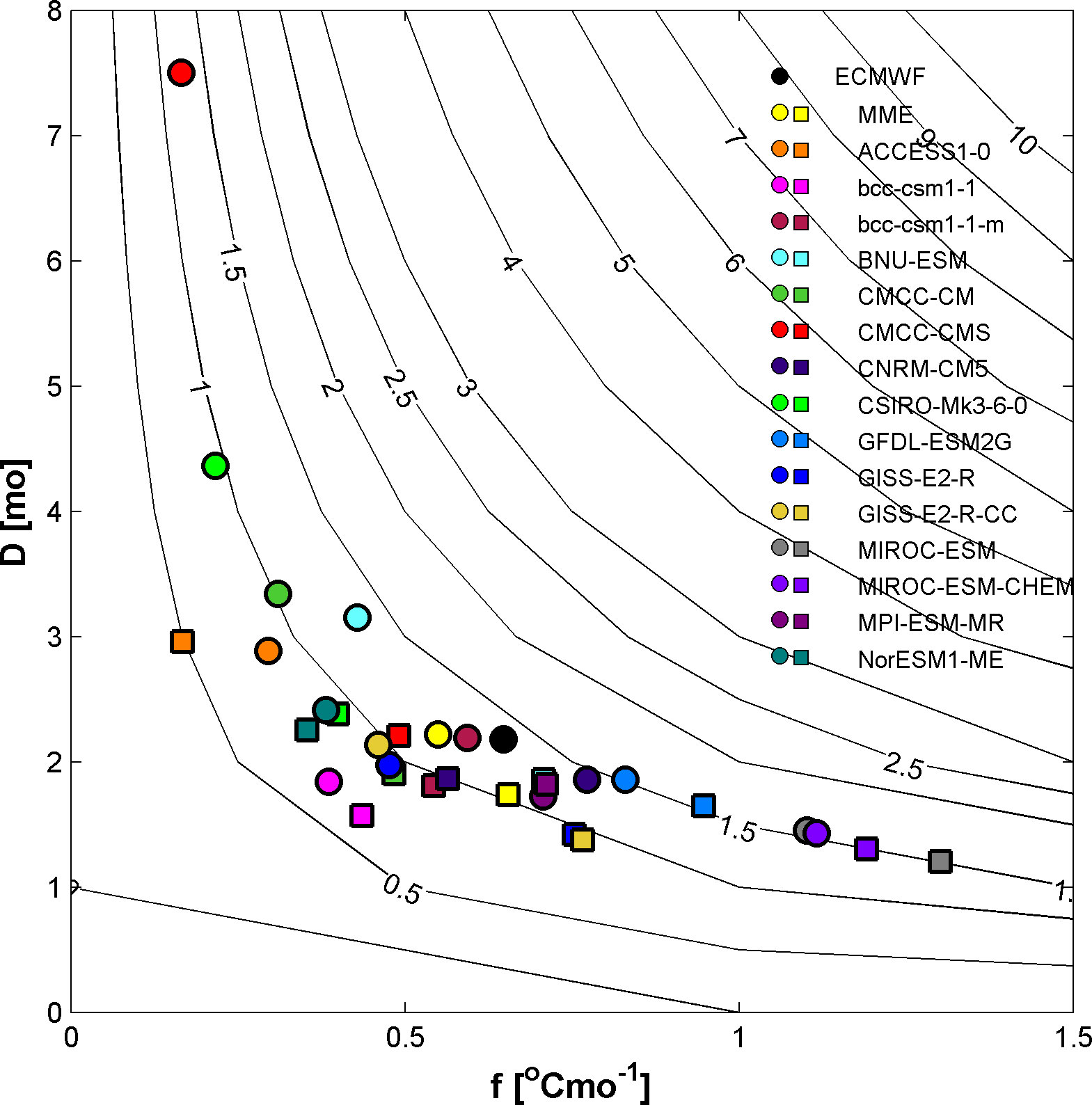
Figure 9 Scatterplots of SSTAC amplitudes (°C) as a function of the dynamical response factor D (month) and total external forcing f (°C month-1) from ECMWF reanalysis dataset (black circle), MME and each of 15 models in the historical period (colored circles) and RCP4.5 scenario (colored squares).
The response of SSTAC in the eastern equatorial Pacific to global warming is investigated using 15 CMIP5 CGCMs under the historical and RCP4.5 scenarios. Historical and RCP4.5 simulations represent the present-day and global-warming climates, respectively. First, we examine pattern formations in SSTAC response to global warming. Compared with observations, the simulated SSTACs of two clime scenarios have weaker amplitudes and are displaced systematically westward. The warm phase occurs nearly one month later and the cold phase decays more rapidly. In future climate, 4 of 15 models simulate a weakening of the seasonal cycle, 4 of 15 models simulate a strengthening of the seasonal cycle and the remaining 7 of 15 models show no significantly changing compared to present-day climate. The annual harmonic component of the seasonal cycle weakens in nearly half of the models, and the semi-annual harmonic component commonly strengthens in most models.
To better evaluate the response of the SSTAC to enhanced CO2 concentration in the future climate, we conduct a coupled dynamic diagnostics framework to diagnose its four main controlling factors, damping rate, propagation speed and external forcing factors. Compared with observations, most simulated SSTACs of two clime scenarios have lower damping rates, comparable propagation speeds, lower annual external forcing and higher semi-annual external forcing. Under global warming, most models exhibit relatively stronger annual and semi-annual external forcing and relatively weaker propagation speed compared to the present-day climate. The damping rate is relatively stronger in half of the models while weaker in the rest. These differences in four controlling factors between two climate periods and between the observation and models are largely attributed to the thermodynamic feedback, especially from the contribution of the short wave radiation.
By combining the damping rate and propagation speed into one dynamical response factor and the two forcings into one forcing factor, we demonstrate that the changes in the SSTAC amplitude under global warming can be simply measured by the forcing factor and the dynamical response factor multiplied together (f·D). Our analysis results show that under global warming, most models have SSTAC amplitudes close to that in the present-day climate, while their dynamical and external forcing factors have obvious changes. Some models’ agreement in the annual cycle amplitudes between the two climate periods may stem from the adjustments and compensations of internal dynamics and external forcing from underlying processes.
The datasets presented in this study can be found in online repositories. The names of the repository/repositories and accession number(s) can be found below: https://pcmdi.llnl.gov/ and http://apdrc.soest.hawaii.edu/.
YC conceived the study, developed the theoretical framework and wrote the manuscript. KY assisted with the analysis and reviewed the manuscript. All authors contributed to the article and approved the submitted version.
This research was supported by Fundamental Research Funds for the Central Universities (Grant B220201024), the Open Fund of State Key Laboratory of Satellite Ocean Environment Dynamics, Second Institute of Oceanography (Grant QNHX2120), the National Science Foundation of China (Grant 41806017), and the Natural Science Foundation of Jiangsu Province (Grant BK20180800).
The authors are grateful to the ESG-PCMDI for providing the CMIP5 historical and RCP4.5 simulations. The ECWMF ORA-S3 and ERA40 datasets were downloaded from Asia Pacific Data Research Center (APDRC) of International Pacific Research Center (IPRC).
The authors declare that the research was conducted in the absence of any commercial or financial relationships that could be construed as a potential conflict of interest.
All claims expressed in this article are solely those of the authors and do not necessarily represent those of their affiliated organizations, or those of the publisher, the editors and the reviewers. Any product that may be evaluated in this article, or claim that may be made by its manufacturer, is not guaranteed or endorsed by the publisher.
Alexander M. A., Scott J. D., Friedland K. D., Mills K. E., Thomas A. C. (2018). Projected sea surface temperatures over the 21st century: Changes in the mean, variability and extremes for large marine ecosystem regions of northern oceans. Elementa Scie Anthropocene 6 (1), 9. doi: 10.1525/elementa.191
An S. I., Jin F.-F., Kang I. S. (1999). The role of zonal advection feedback in phase transition and growth of ENSO on the cane-zebiak model. J. Met Soc. Japan 77, 1151–1160. doi: 10.2151/jmsj1965.77.6_1151
Balmaseda M. A., Vidard A., Anderson D. L. (2008). ECMWF ocean analysis system: ORA-S3. Mon Wea Rev. 136, 3018–3034. doi: 10.1175/2008MWR2433.1
Biasutti M., Sobel A. H. (2009). Delayed sahel rainfall and global seasonal cycle in a warmer climate. Geophys. Res. Lett. 36, L23707. doi: 10.1029/2009GL041303
Brander K. (2013). Climate and current anthropogenic impacts on fisheries. Climatic Change 119 (1), 9–21. doi: 10.1007/s10584-012-0541-2
Cane M. A., Clement A.C., Kaplan A., Kushnir Y., Pozdnyakov D., Seager R., et al (1997). Twentieth-century sea surface temperature trends. Science 275 (5302), 957–960. doi: 10.1126/science.275.5302.957
Carton J. A., Ding Y., Arrigo K. R. (2015). The seasonal cycle of the Arctic ocean under climate change. Geophys. Res. Lett. 42, 7681–7686. doi: 10.1002/2015GL064514
Chang P., Philander S. G. H. (1994). A coupled ocean-atmosphere instability of relevance to the seasonal cycle. J. Atmos. Sci. 51, 3627–3648. doi: 10.1175/1520-0469(1994)051<3627:ACOIOR>2.0.CO;2
Chen Y.-Y., Jin F.-F. (2017). Dynamical diagnostics of the SST annual cycle in the Eastern equatorial pacific: Part II analysis of CMIP5 simulations. Clim. Dyn. 49 (11-12), 3923–3936. doi: 10.1007/s00382-017-3550-z
Chen Y.-Y., Jin F.-F. (2018). Dynamical diagnostics of the SST annual cycle in the eastern equatorial pacific: part I a linear coupled framework. Clim. Dyn. 50 (5-6), 1841–1862. doi: 10.1007/s00382-017-3725-7
Clement A. C., Seager R., Cane M. A., Zebiak S. E. (1996). An ocean dynamic thermostat. J. Clim. 9, 2190–2196. doi: 10.1175/1520-0442(1996)009<2190:AODT>2.0.CO;2
Collins M., Modeling Groups C. M. I. P. (2005). El Nino-or la Nina-like climate change? Clim. Dyn. 24, 89–104. doi: 10.1007/s00382-004-0478-x
Deutsch C., Ferrel A., Seibel B., Pörtner H. O., Huey R. B. (2015). Climate change tightens a metabolic constraint on marine habitats. Science 348, 1132–1135. doi: 10.1126/science.aaa1605
DiNezio P. N., Clement A. C., Vecchi G. A., Soden B. J., Kirtman B. P., Lee S.-K. (2009). Climate response of the equatorial pacific to global warming. J. Clim. 22, 4873–4892. doi: 10.1175/2009JCLI2982.1
Doney S. C., Ruckelshaus M., Duffy J. E., Barry J. P., Chan F., English C., et al. (2012). Climate change impacts on marine ecosystems. Ann. Rev. Mar. Sci. 4, 11–37. doi: 10.1146/annurev-marine-041911-111611
Drinkwater K. F., Beaugrand G., Kaeriyama M., Kim S., Ottersen G., Perry R., et al. (2010). On the processes linking climate to ecosystem changes. J. Mar. Sys 79, 374–388. doi: 10.1016/j.jmarsys.2008.12.014
Dwyer J. G., Biasutti M., Sobel A. H. (2012). Projected changes in the seasonal cycle of surface temperature. J. Clim 25, 6359–6374. doi: 10.1175/JCLI-D-11-00741.1
Hanson K. J., Hasler A. F., Kornfield J., Suomi V. E. (1967). Photographic cloud climatology from ESSA III and V computer produced mosaics. Bull. Am. Meteorol. Soc. 48, 878–883. doi: 10.1175/1520-0477-48.12.878
Hollowed A. B., Barange M., Beamish R., Brander K., Cochrane K., Drinkwater K., et al. (2013). Projected impacts of climate change on marine fish and fisheries. ICES J. Mar. Sci. 70 (5), 1023–1037. doi: 10.1093/icesjms/fst081
Horel J. D. (1982). On the annual cycle of the tropical pacific atmosphere and ocean. Mon Wea Rev. 110, 1863–1878. doi: 10.1175/1520-0493(1982)110<1863:OTACOT>2.0.CO;2
Jin F.-F. (1996). Tropical ocean-atmosphere interaction, the pacific cold tongue, and the El niño southern oscillation. Science 274, 76–78. doi: 10.1126/science.274.5284.76
Jin F.-F., Kim S. T., Bejarano L. (2006). A coupled-stability index for ENSO. Geophys. Res. Lett. 33, L23708. doi: 10.1029/2006GL027221
Jin F.-F., Neelin J. D. (1993). Modes of interannual tropical ocean-atmosphere interaction-a unified view. part I: Numerical results. J. Atmos Sci. 50, 3477–3503. doi: 10.1175/1520-0469(1993)050<3477:MOITOI>2.0.CO;2
Jin F.-F., Neelin J. D., Ghil M. (1994). El Niño on the devil's staircase: annual and subharmonic steps to chaos. Science 264, 70–72. doi: 10.1126/science.264.5155.70
Liu F., Lu J., Luo Y., Huang Y., Song F. (2020). On the oceanic origin for the enhanced seasonal cycle of SST in the midlatitudes under global warming. J. Clim. 33 (19), 8401–8413. doi: 10.1175/JCLI-D-20-0114.1
Liu F., Luo Y., Lu J., Wan X. (2017). Response of the tropical pacific ocean to El niño versus global warming. Clim. Dyn. 48, 935–956. doi: 10.1007/s00382-016-3119-2
Liu Z., Vavrus S., He F., Wen N., Zhong Y. (2005). Rethinking tropical ocean response to global warming: the enhanced equatorial warming. J. Clim. 18, 4684–4700. doi: 10.1175/JCLI3579.1
Manabe S., Hahn D. G., Hollaway J. (1974). The seasonal variation of tropical circulation as simulated by a global model of atmosphere. J. Atmos. Sci. 32, 43–83. doi: 10.1175/1520-0469(1974)031<0043:TSVOTT>2.0.CO;2
Mitchell T. P., Wallace J. M. (1992). The annual cycle in equatorial convection and sea-surface temperature. J. Clim. 5, 1140–1156. doi: 10.1175/1520-0442(1992)005<1140:TACIEC>2.0.CO;2
Neelin J. D. (1991). The slow sea surface temperature mode and the fast-wave limit: Analytic theory for tropical interannual oscillations and experiments in a hybrid coupled model. J. Atmos. Sci. 48, 584–606. doi: 10.1175/1520-0469(1991)048<0584:TSSSTM>2.0.CO;2
Ottersen G., Kim S., Huse G., Polovina J. J., Stenseth N. C. (2010). Major pathways by which climate may force marine fish populations. J. Mar. Sys 79, 343–360. doi: 10.1016/j.jmarsys.2008.12.013
Philander S. G. H., Gu D., Halpern D., Lambert G., Lau N. C., Li T., et al. (1996). Why the ITCZ is mostly north of the equator. J. Clim. 9, 2958–2972. doi: 10.1175/1520-0442(1996)009<2958:WTIIMN>2.0.CO;2
Philander S. G. H., Seigel A. D. (1985). “Simulation of El niño of 1982-1983,” in Coupled ocean-atmosphere models, vol. 40 . Ed. Nihoul J. C. J. (Elsevier Oceanogr Ser), 517–541.
Rivkin R. B., Legendre L. (2001). Biogenic carbon cycling in the upper ocean: effects of microbial respiration. Science 291 (5512), 2398–2400. doi: 10.1126/science.291.5512.2398
Sobel A. H., Camargo S. J. (2011). Projected future seasonal changes in tropical summer climate. J. Clim. 24 (2), 473–487. doi: 10.1175/2010JCLI3748.1
Stine A. R., Huybers P. (2012). Changes in the seasonal cycle of temperature and atmospheric circulation. J. Clim. 25, 7362–7380. doi: 10.1175/JCLI-D-11-00470.1
Stuecker M. F., Jin F.-F., Timmermann A. (2015). El Niño-Southern oscillation frequency cascade. Proc. Nat. Acad. Sci. 112 (44), 13490–13495. doi: 10.1073/pnas.1508622112
Stuecker M. F., Timmermann A., Jin F.-F., McGregor S., Ren H.-L. (2013). A combination mode of the annual cycle and the El Niño/Southern oscillation. Nat. Geosci. 6, 540–544. doi: 10.1038/ngeo1826
Taylor K. E., Stou_er R. J., Meehl G. A. (2011). An overview of CMIP5 and the experiment design. Bull. Am. Meteorol. Soc. 93 (4), 485–498. doi: 10.1175/BAMS-D-11-00094.1
Timmermann A., Jin F.-F., Collins M. (2004). Intensification of the annual cycle in the tropical pacific due to greenhouse warming. Geophys. Res. Lett. 31, L12208. doi: 10.1029/2004GL019442
Tziperman E., Stone L., Cane M. A., Jarosh H. (1994). El Niño chaos: Overlapping of resonances between the seasonal cycle and the pacific ocean-atmosphere oscillator. Science 263, 72–74. doi: 10.1126/science.264.5155.72
Uppala S. M., Kållberg P. W., Simmons A. J., Andrae U., Bechtold V. D. C., Fiorino M., et al. (2005). The ERA-40 re-analysis. Quart J. Roy Meteor. Soc. 131, 2961–3012. doi: 10.1256/qj.04.176
Wang B. (1994). On the annual cycle in the tropical eastern central pacific. J. Clim. 7, 1926–1942. doi: 10.1175/1520-0442(1994)007<1926:OTACIT>2.0.CO;2
Wengel C., Latif M., Park W., Harlass J., Bayr T. (2018). Seasonal ENSO phase locking in the Kiel climate model: The importance of the equatorial cold sea surface temperature bias. Clim. Dyn. 50 (3-4), 901–919. doi: 10.1007/s00382-017-3648-3
Wyrtki K., Meyers G. (1976). The trade wind field over the pacific ocean. J. Appl. Meteor. 15, 698–704. doi: 10.1175/1520-0450(1976)015<0698:TTWFOT>2.0.CO;2
Xie S. P. (1994). On the genesis of the equatorial annual cycle. J. Clim 7, 2008–2013. doi: 10.1175/1520-0442(1994)007<2008:OTGOTE>2.0.CO;2
Xie S. P. (2004). “The shape of continents, air-sea interaction, and the rising branch of the Hadley circulation,” in The Hadley circulation: present, past and future. Eds. Diaz H. F., Bradley R. S. (Kluwer Academic Publishers), 121–152.
Xie S. P., Deser C., Vecchi G. A., Ma J., Teng H., Wittenberg A. T. (2010). Global warming pattern formation: sea surface temperature and rainfall. J. Clim. 23, 966–986. doi: 10.1175/2009JCLI3329.1
Keywords: global warming, SST annual cycle, westward propagation, external forcing, CMIP
Citation: Chen Y-Y and Yu K (2022) The responses of SST annual cycle in the eastern equatorial Pacific to global warming. Front. Mar. Sci. 9:1100510. doi: 10.3389/fmars.2022.1100510
Received: 16 November 2022; Accepted: 05 December 2022;
Published: 22 December 2022.
Edited by:
Hui Zhao, Guangdong Ocean University, ChinaReviewed by:
Yi Yu, Ministry of Natural Resources, ChinaCopyright © 2022 Chen and Yu. This is an open-access article distributed under the terms of the Creative Commons Attribution License (CC BY). The use, distribution or reproduction in other forums is permitted, provided the original author(s) and the copyright owner(s) are credited and that the original publication in this journal is cited, in accordance with accepted academic practice. No use, distribution or reproduction is permitted which does not comply with these terms.
*Correspondence: Kai Yu, eXVrYWkwNDFAaGh1LmVkdS5jbg==
Disclaimer: All claims expressed in this article are solely those of the authors and do not necessarily represent those of their affiliated organizations, or those of the publisher, the editors and the reviewers. Any product that may be evaluated in this article or claim that may be made by its manufacturer is not guaranteed or endorsed by the publisher.
Research integrity at Frontiers
Learn more about the work of our research integrity team to safeguard the quality of each article we publish.