Decadal variability of sea surface salinity in the Southeastern Indian Ocean: Roles of local rainfall and the Indonesian throughflow

The southeastern Indian Ocean (SEIO) exhibits prominent decadal variability in sea surface salinity (SSS), showing salinity decreases during 1995-2000 and 2005-2011 and increases during 2000-2005 and after 2011. These salinity changes are linked to the Indo-Pacific climate and have impacts on the regional marine environment. Yet, the underlying mechanism has not been firmly established. In this study, decadal SSS variability of the SEIO is successfully simulated by a high-resolution regional ocean model, and the mechanism is explored through a series of sensitivity experiments. The results suggest that freshwater transport of the Indonesian throughflow (ITF) and local precipitation are two major drivers for the SSS decadal variability. They mutually cause most of the variability, with a generally larger contribution of precipitation. Other processes, such as evaporation and advection driven by local winds, play a minor role. Further analysis shows that the decadal precipitation in the SEIO is mainly associated with the decadal variability of Ningaloo Niño. Ocean dynamic processes significantly modify the relationship between SSS and precipitation, greatly shortening their lag time. The changes in both volume transport and salinity of the ITF water can cause large salinity changes in the SEIO region. Although local wind forcing gives rise to considerable changes in evaporation rate and ocean current advection, its overall contribution to decadal SSS variability is small compared to local precipitation and the ITF.

1. Introduction

Changes in ocean salinity are an essential aspect of climate change and effective indicators for measuring alterations in the global water cycle (e.g., Yu, 2011; Durack et al., 2012; Yu et al., 2020). Evaporation and precipitation over the oceans are major components of the global water cycle (Durack, 2015) and constitute the bulk of surface freshwater fluxes. The surface freshwater flux, e.g., evaporation minus precipitation (E - P), plays a fundamental role in shaping the large-scale distribution of sea surface salinity (SSS) in climatology. Existing studies attempted to explore changes in the global water cycle by analyzing changes in ocean salinity (e.g., Delcroix et al., 2007; Schmitt, 2008; Hosoda et al., 2009; Helm et al., 2010; Yu, 2011; Durack et al., 2012; Terray et al., 2012; Skliris et al., 2016; Zika et al., 2018). The global water cycle has been suggested to strengthen owing to anthropogenic greenhouse warming (e.g., Helm et al., 2010; Durack et al., 2012). Correspondingly, SSS shows a trend pattern of ‘salty gets saltier; fresh gets fresher’ (e.g., Yu, 2011; Durack et al., 2012; Cheng et al., 2020). While these long-term trends of broad-scale salinities have been predominantly attributed to freshwater fluxes associated with anthropogenic climate change, the short-term (interannual and decadal) variabilities of regional salinities are subjected to complexity and diversity in characteristics and mechanisms. Multiple physical processes of comparable importance may operate in these regional variabilities.

The Southeast Indian Ocean (SEIO) possesses active ocean-atmosphere interactions (e.g., Saji and Yamagata, 2003; Tozuka et al., 2013; Li et al., 2019) and receives strong influences of the Indonesian Throughflow (ITF) (e.g., Wijffels and Meyers, 2004; Qu and Meyers, 2005a). Salinity variability in the SEIO region exerts notable impacts on ocean stratification, sea level, ITF transport, and local circulation (e.g., Masson et al., 2002; Qu and Meyers, 2005; Llovel and Lee, 2015; Zhang et al., 2016a; Zhang et al., 2017; Hu and Sprintall, 2016; Li et al., 2020; Lu et al., 2022). In the sea-level rise of SEIO since the 1960s, the contribution of salinity change through the halosteric effect reached ~40% (Lu et al., 2022). The salinity decline in the upper SEIO since 2005 greatly enhanced the recent sea-level rise (Llovel and Lee, 2015; Li et al., 2017; Huang et al., 2020). Menezes et al. (2013) pointed out that the meridional salinity gradient in the SEIO is essential for the formation of the Eastern Gyral Current. Hu and Sprintall (2016; 2017) pointed out that salinity changes in the SEIO affect the interannual variability and long-term trends of the ITF transport. These significant aspects highlight the necessity of investigating the prominent salinity variability of the SEIO.

Research efforts have been devoted to understanding the multi-timescale variabilities of the SEIO salinity. Regarding the seasonality, the tropical SEIO surface salinity decreases in austral winter (“austral” omitted hereafter) and increases in summer, as dictated by surface freshwater flux (Qu and Meyers, 2005; Zhang et al., 2016a). On interannual timescales, El Niño (La Niña) events tend to cause SSS increases (decreases) in the SEIO, respectively, through the teleconnection signatures on rainfall and ocean circulation of the SEIO (e.g., Zhang et al., 2016a; Hu et al., 2019; Guo et al., 2021). The SEIO is also a region with pronounced decadal variability (e.g., Feng et al., 2010; Du et al., 2015; Feng et al., 2015; Li et al., 2017; Hu et al., 2019; Li et al., 2019; Li et al., 2022). The SEIO region showed a persistent SSS decrease during 2005-2013 (e.g., Du et al., 2015; Nie et al., 2020). Du et al. (2015) linked this decadal freshening to the slowdown of global surface warming (also dubbed the “hiatus”; e.g., Meehl et al., 2011) and the enhancement of the Pacific Walker Circulation (e.g., England et al., 2014). Other studies pointed out that the upper-ocean salinity of SEIO does not monotonically decrease but shows decadal fluctuations, with salinity increases occurring both before and after the 2005-2013 period (e.g., Hu et al., 2019; Guo et al., 2021; Wu et al., 2021).

Various datasets and approaches have been utilized to explore the mechanisms of the decadal salinity variability in the SEIO (e.g., Du et al., 2015; Zhang et al., 2017; Hu et al., 2019; Huang et al., 2020; Wu et al., 2021). By analyzing Argo data, Du et al. (2015) showed that changes in precipitation and advection of ocean circulation were responsible for the SSS decline during 2005-2013. Zhang et al. (2016b) revealed a salinity dipole mode of the Indian Ocean, with the SEIO region acting as the eastern pole. This dipole mode also shows decadal variability, in which fresh-water transport from lower latitudes and thermocline variability imported by the ITF control SSS changes in the SEIO (Zhang et al., 2017). Hu et al. (2019) performed a salt budget analysis using an ocean reanalysis product. They showed that horizontal advection by the ITF and the South Equatorial Current (SEC) are the main drivers of interannual and decadal changes in the SEIO salinity, while surface freshwater fluxes play a secondary role. The salt budget analysis of Huang et al. (2020) suggested that the salinity gradient between tropical low-salinity water and subtropical high-salinity water is favorable for strong meridional salinity advection anomalies, which is conducive for decadal salinity variability. Wu et al. (2021) also suggested the essence of meridional salinity advection and attributed it to local wind forcing. Thereby, they emphasized the importance of local oceanic and atmospheric processes rather than the remote forcing by the Pacific. One can see that previous studies have identified multiple processes regulating the decadal SSS variability of the SEIO. Yet, a consensus on their relative importance is still lacking.

In this study, the eddy-resolving hindcast of a regional ocean model successfully simulated the SSS variability in the SEIO, and a series of sensitivity experiments were used to assess the contribution of different processes. Different from existing studies that widely adopt the salt budget, the sensitivity experiments allow us to isolate the effect of each process (e.g., precipitation, winds, ITF, etc.) in a clean manner and clarify the sources of changes. This provides unambiguous insights into the mechanisms governing the SSS variability. Our efforts contribute to the understanding and prediction of the salinity dynamics and related changes in sea level, stratification, and circulation of the SEIO. The rest of this article is organized as follows. Section 2 presents the datasets and methods used in this study. Section 3 describes the spatial and temporal characteristics of the observed SSS variability and model simulations. Section 4 explores the key processes underlying the decadal SSS variability, focusing on the effects of local rainfall and the ITF. Conclusions and discussion are provided in Section 5.

2. Data and model

2.1. Observation data

Observational ocean datasets utilized in this study include the 1^o×1^o monthly salinity data of the International Pacific Research Center (IPRC) gridded Argo product (Lebedev et al., 2007) for 2005-2016, and the 1^o×1^o monthly Institute of Atmospheric Physics (IAP) ocean salinity product of 1993-2016. The IAP salinity product was constructed using a mapping technology of Ensemble Optimal Interpolation (EnOI) (Cheng et al., 2017) and incorporating dynamic training with simulations by phase 5 of the Coupled Model Intercomparison Project (CMIP5; Taylor et al., 2012). Cheng et al. (2020) showed that the IAP salinity data product can overcome the shortcomings of earlier reconstructions such as ‘no-data, no-signal’ and has uncertainties better constrained. To explore the atmospheric forcing effects, we also analyzed the 0.75^o×0.75^o monthly precipitation rate and 10-m wind data from the interim European Centre for Medium-Range Weather Forecasts (ECMWF) Re-Analysis (ERA-Interim) for 1993-2016 (Dee et al., 2011). For all datasets, the anomaly of a variable is obtained by removing the monthly climatology. Among them, the monthly climatology of 2005-2016 is removed from the Argo data, while that of 1993-2016 is removed from the IAP and ERA-Interim data. To represent decadal variability of the Pacific climate, we compute the Interdecadal Pacific Oscillation (IPO) index using the monthly Met Office's Hadley Centre Sea Ice and Sea Surface Temperature (HadISST; Rayner, 2003). Following Henley et al. (2015), the IPO index is computed as the sea surface temperature (SST) anomaly difference between the equatorial Pacific (170°E-90°W, 10°S-10°N) and the northwest plus the southwest Pacific Ocean (140°E-145°W, 25°-45°N plus 150°E-160°W, 50°-15°S).

2.2. ROMS

We adopt the regional oceanic modeling system (ROMS) to carry out hindcasts for the SEIO salinity. ROMS is a hydrostatic, primitive equation model that implements a free surface, horizontal curvilinear coordinate, and a terrain-following (sigma-type) vertical coordinate system (e.g., Haidvogel et al., 2000). The model domain covers a sector-shaped region between 80°-122°E, 42°S-5°N, bordered by the Western Australian coast to the east and Sumatra-Java islands to the north (Guo et al., 2021; Li et al., 2022). The horizontal resolution is ~3 km near the Western Australian coast and degrades to ~12 km near the western boundary at 80°. As such, the enhanced mesoscale eddy variability in the Leeuwin Current system (e.g., Feng et al., 2005; Feng et al., 2007; Jia et al., 2011; Guo et al., 2020b) and complex coastal dynamics in the SEIO can be better resolved. There are 600 × 560 horizontal grid points and 30 sigma-type vertical layers over the entire model domain.

The 3-hourly ERA-Interim fields, including 10-m winds, precipitation, radiations, and 2-m air temperature and humidity, are used as surface atmospheric forcing, while the ¹/₁₂° Hybrid Coordinate Ocean Model (HYCOM) plus Navy Coupled Ocean Assimilation global reanalysis (Cummings, 2006) are adopted to provide the lateral boundary conditions. A strong relaxation toward climatology is exerted on lateral boundaries to damp artificial boundary waves. Readers are referred to Guo et al. (2021) for more detailed configurations. The spin-up of ROMS is 20 years, under monthly climatological surface atmospheric forcing and lateral boundary conditions. Then, the model was integrated forward under 3-hourly atmospheric fields and daily lateral boundary conditions from January 1993 to December 2016. This experiment includes the complete forced and internal processes affecting salinity, which is addressed as the control run (Ctr).

In addition to Ctr, sensitivity experiments were performed from January 1993 through December 2016 [see Table 1 of Guo et al. (2021) for the list]. The Exp-B adopts monthly climatology in all atmospheric forcing fields but realistic lateral boundary conditions as in Ctr. As such, Exp-B retains only the forcing effect from the lateral boundaries, as indicated by the “B” (for boundary) in its naming. As has been validated by previous studies (Guo et al., 2021; Li et al., 2022), variability in Exp-B mainly originates from the ITF. In other experiments, atmospheric forcing is exerted in addition to the ITF effect. For example, Exp-BW adopts realistic 3-hourly winds as in Ctr but fixes other forcing fields to monthly climatology. As such, Exp-BW measures the combined effect of both the ITF and local wind forcing (“W”). The difference between Exp-BW and Exp-B, e.g., Exp-BW minus Exp-B, roughly represents the local wind forcing effect. The Exp-BP experiment includes the effect of local precipitation ("P") and measures the joint effect of the ITF and precipitation. Exp-BP minus Exp-B isolates the effect of local precipitation (mainly rainfall in the SEIO). The Exp-BWTQ experiment adopts the realistic fields in winds (“W”), atmospheric temperature (“T”), and humidity (“Q”). As such, it contains all the atmospheric variability influential for evaporation.

The ITF’s effect on the SEIO salinity depends on not only the amount (volume transport) but also the salinity of its water. To distinguish these two effects, the Exp-Bv experiment is devised. Exp-Bv is the same as Exp-B except using the monthly climatological salinity in lateral boundary conditions so that it isolates the effect of the ITF’s velocity change (or volume transport change). Meanwhile, Exp-B minus Exp-Bv represents the salinity change of the ITF water.

3. Decadal SSS variability and ROMS simulation

We first compare the monthly SSS anomaly (SSSA) time series of the SEIO region (14^o-28^oS, 95^o-115^oE) from observational data (Argo and IAP) and ROMS Ctr (Figure 1A). The SSSA simulated by ROMS Ctr exhibits quite the same temporal evolution as those in observations. During the Argo era of 2005-2016, Ctr shows a correlation coefficient of 0.90 with Argo and a correlation of 0.92 with IAP, significant at the 95% confidence level. The standard deviation of SSSA is 0.12 psu for Ctr, quite close to those in IAP and Argo (0.12 and 0.13 psu, respectively), indicating similar variability amplitudes. It is worth noting that the three sets of data IAP and Ctr are highly consistent after 2005 but show evident discrepancies in many years before. Over the 1993-2004 period, the correlation between Ctr and IAP is 0.56. They are generally in phase, but the correlation is evidently lower than that after 2005. This is probably due to the insufficient data sampling to constrain the salinity estimate of IAP prior to the Argo era.

FIGURE 1

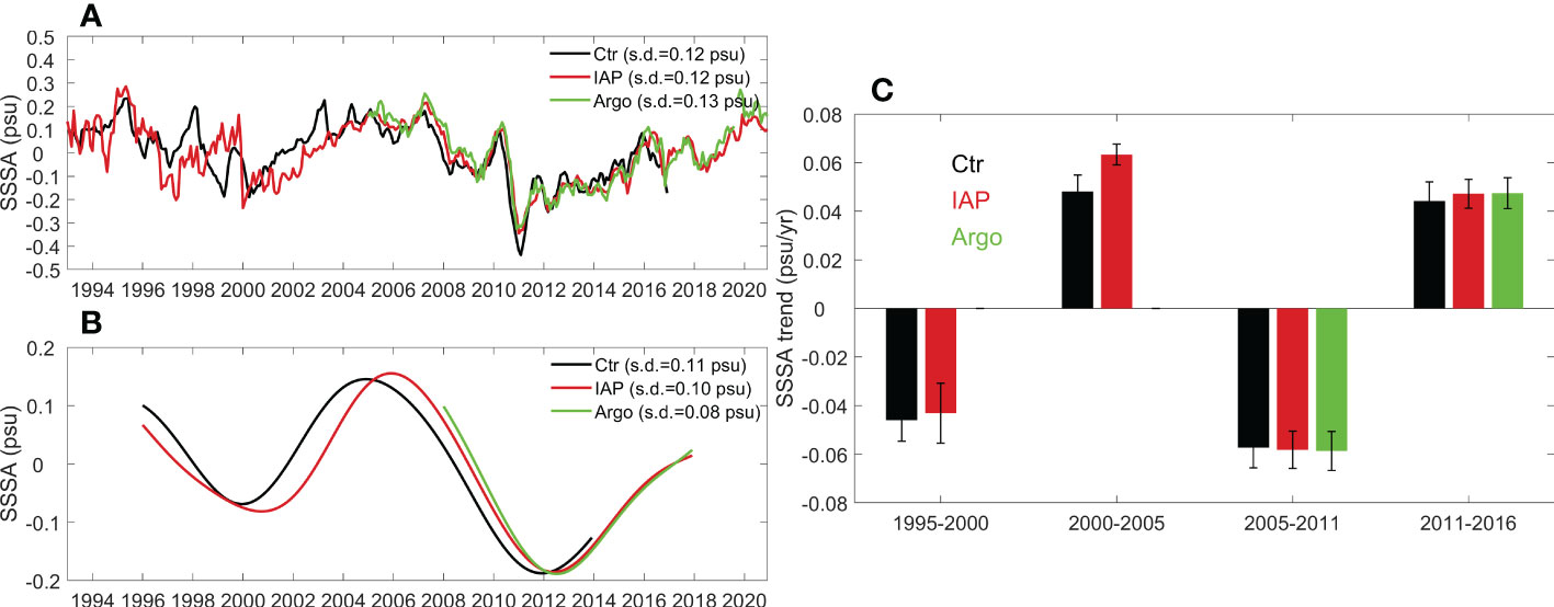
Figure 1 (A) Time series of monthly sea surface salinity anomaly (SSSA; in psu) averaged over the SEIO region (14^o-28^oS, 95^o-115^oE) from ROMS Ctr (black), IAP (red), and gridded Argo data (green). The standard deviation is also shown in the legend box. (B) As in (A), but for 6-yr low-pass-filtered SSSA. (C) Linear trends of SSS in the SEIO for the periods of 1995-2000, 2000-2005, 2005-2011, and 2011-2016 derived from Ctr (black), IAP (red) and Argo (green). Error-bars denote the 90% confidence interval based on an F test.

Both the observed and simulated SSSA show prominent decadal variations, including a salinity decrease from 1995 to 2000, an increase from 2000 to 2005, a decrease from 2005 to 2011, and a salinity increase after 2011. To highlight these decadal changes, we smoothed the SSSA using a 6-year low-pass Lanczos digital filter (Figure 1B). The above-mentioned decadal changes are clearly discernible in all the three datasets. Choosing a wider window for the filter (e.g., 7 or 8 years) yields roughly the same results. Decadal SSS variability in Figures 1A, 1B generally shows two cycles during 1995-2020, indicating a typical period of ~13 years. To better quantify the decadal variability, we calculated linear trends of the four periods (Figure 1C). The trends derived from the three datasets are also close; for example, during 2005-2011, the downward trends of SSS were -0.057, -0.058, -0.059 psu yr^-1 in of Ctr, IAP and Argo, respectively. During 2000-2005, the SSS increase in Ctr is weaker than that in IAP data (0.048 versus 0.063 psu yr^-1, respectively). These comparisons overall suggest the fidelity of ROMS in simulating of the decadal salinity variability.

We then examine the SSS climatology of 1995-2016, which is the background for the generation of salinity variability. Figure 2 suggests that ROMS can realistically simulate the SSS distribution, with the low-salinity water in the tropical sector and the high-salinity water in the subtropical sector (e.g., Huang et al., 2020; Wu et al., 2021). There is a zonal SSS front formed approximately between 15^o-25^oS, and the cross-front salinity difference exceeds 1.6 psu (from 34.2 psu in the north to 35.8 psu in the south). This front is stronger in fall (April) and weaker in spring (October) in Ctr, which is however less obvious in IAP. The center of the subtropical salty salinity (Wang et al., 2020) locates at ~30^oS, showing an SSS maximum~36.0 psu in ROMS simulation. The low-salinity tropical water is confined north of 15^oS, with an SSS minimum of ~34.0 psu.

FIGURE 2

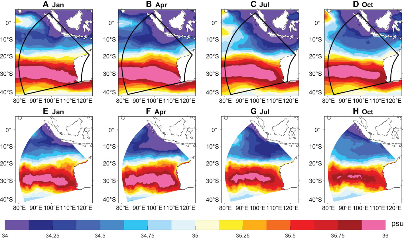
Figure 2 Monthly climatology of SSS (psu) in January, April, July, and October of 1995-2016 derived from IAP (A-D) and ROMS Ctr (E-H).

The spatial patterns of SSS trends over the four periods are shown in Figure 3. Salinity changes are strongest along the Western Australian coast and extend westward with decreasing amplitudes. Significant changes can extend to the western boundary of the model domain between 20^o-24^oS. Meanwhile, the Sumatra-Java coasts and the subtropical area south of 30^oS tend to show opposite salinity changes, except for the 2000-2005 period. These spatial patterns are faithfully captured by ROMS (Figures 3E–H). The trend maps for a larger area derived from IAP data (Figures 3A–D) indicate that SSS changes in the SEIO are connected to those in Indonesian Seas and are out-of-phase to those in the western tropical Pacific. Therefore, changes in the SEIO are likely linked to the tropical Pacific climate (e.g., Du et al., 2015; Hu et al., 2019).

FIGURE 3

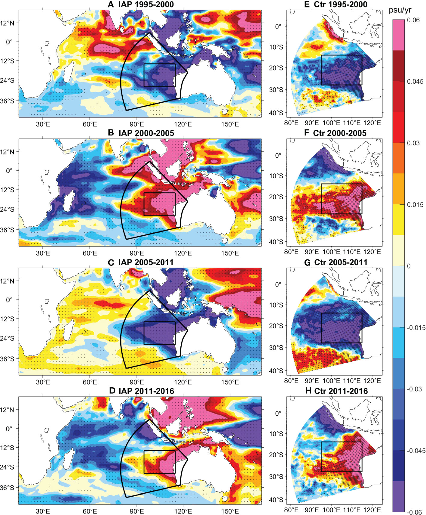
Figure 3 Linear trend maps of SSS for the periods of (A) 1995-2000, (B) 2000-2005, (C) 2005-2011, and (D) 2011-2016 derived from IAP. (E–H) As in (A–D), but for derived from Ctr, respectively. Stippling indicates significant trends at 90% confidence level based on a Mann-Kendall test. Black lines denote the model domain (sector shape) and the SEIO region (rectangle).

4. The underlying mechanism

4.1. Key processes

The mechanism governing SSS variability in the SEIO is complex and likely regulated by multiple processes (e.g., Du et al., 2015; Hu et al., 2019; Huang et al., 2020; Guo et al., 2021; Wu et al., 2021). In this section, we attempt to quantitatively evaluate the effects of different processes. Validations provided in Chapter 3 and previous studies (e.g., Guo et al., 2020a; Guo et al., 2020b; Guo et al., 2021) demonstrate that ROMS can realistically simulate the SEIO salinity variability, placing confidence for the usage of ROMS experiments to explore the mechanism.

The Exp-BP experiment contains the combined effect of the ITF and local precipitation. Its result is highly consistent with Ctr in SSS, with a correlation coefficient of 0.96 (Figure 4A). Its standard deviation is 0.13 psu, even exceeding that of Ctr (0.12 psu). This indicates that the two processes, the ITF and precipitation, drive the majority of the SSS variability, and the overall effect of other processes (such as evaporation and local winds). The Exp-B experiment only retains the variability arising from the ITF. Its result is basically in phase with Ctr, with a correlation of 0.77, and its standard deviation is 0.07 psu, accounting for half of that of Ctr. This confirms that changes in freshwater inflow from the Indonesian Seas contribute significantly to the SSS variability in SEIO. The difference between the two experiments, Exp-BP minus Exp-B, represents the effect of local precipitation. Compared to the ITF, the precipitation effect can better explain the total SSSA in Ctr, with a standard deviation of 0.09 psu and a correlation of 0.83 with Ctr (Figure 4B). Therefore, local precipitation is the leading driver of the large-scale SSS variability in the SEIO, and the role of ITF is overall secondary. Note that the SSS in Figure 4 contains both interannual and decadal variations. The important role of local precipitation in interannual variability is in line with the results of Zhang et al. (2016b).

FIGURE 4

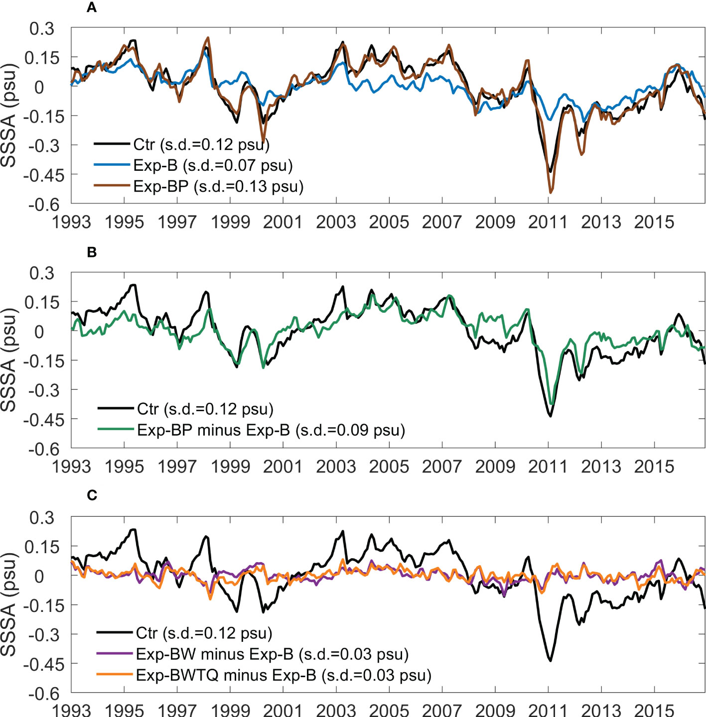
Figure 4 (A) Time series of monthly SSSA (in psu) averaged over the SEIO from Ctr (black), Exp-B (blue), and Exp-BP (brown). (B, C) As in (A), but for Ctr (black), Exp-BP minus Exp-B (green), Exp-BW minus Exp-B (purple), and Exp-BWTQ minus Exp-B (orange). The standard deviation is also shown in the legend box.

We also explored other processes. Exp-BW minus Exp-B represents the forcing effect of local winds. Winds affect ocean salinity through ocean current advection and evaporation. However, our results show that the local wind forced SSSA is relatively weak (Figure 4C). Its standard deviation is 0.03 psu, and its correlation with Ctr is merely 0.18 (insignificant at the 95% confidence level). Evaporation is affected by atmospheric temperature and humidity, and their effects are also contained in Exp-BWTQ. In addition, previous studies (e.g., Zhang et al., 2018; Li et al., 2019; Guo et al., 2020a) have shown that latent heat flux is the leading driver of sea surface temperature (SST) variability in this region, while the contribution of ITF to the interannual and decadal SST variability is <20%. By synthesizing the effects of winds, air temperature, humidity, and the majority of SST variability, Exp-BWTQ minus Exp-B contains most of the change in evaporation. However, its result is quite close to Exp-BW minus Exp-B (standard deviation ~0.03 psu, correlation of 0.26 with Ctr). These results suggest that in comparison with local precipitation and the ITF, the contribution of local winds and evaporation is quite limited. This differs from the conclusions of existing studies based on salinity budget analysis (e.g., Huang et al., 2020; Wu et al., 2021).

For better quantification, we calculated the salinity trends induced by ITF (Exp-B), precipitation (Exp-BP minus Exp-B), and local winds (Exp-BW minus Exp-B) over four periods (Figure 5). The ITF and precipitation are of comparable importance, while the role of local winds is minor. For example, during 1995-2000, the contributions of the ITF and precipitation to the salinity decline are both ~50%, while winds act to slightly damp the salinity decline; for the salinity increase during 2000-2005, the contributions of ITF, precipitation, and winds are 24%, 68%, and 10%, respectively. Although the relative importance of ITF and precipitation varies with time, both are essential and jointly control the decadal trends of SSS. It is also noted that the sum of the contributions of ITF and precipitation significantly exceeds the total change in Ctr during the 2011-2016 period, which is also discernible in Figure 4A. This is largely due to the attenuation effect of other processes, such as evaporation. The result of Exp-BWTQ minus Exp-B indicates that the evaporation change, induced by local winds, air temperature, and humidity, exerts a damping effect on the total SSS increase during 2011-2016 (Figure 5).

FIGURE 5

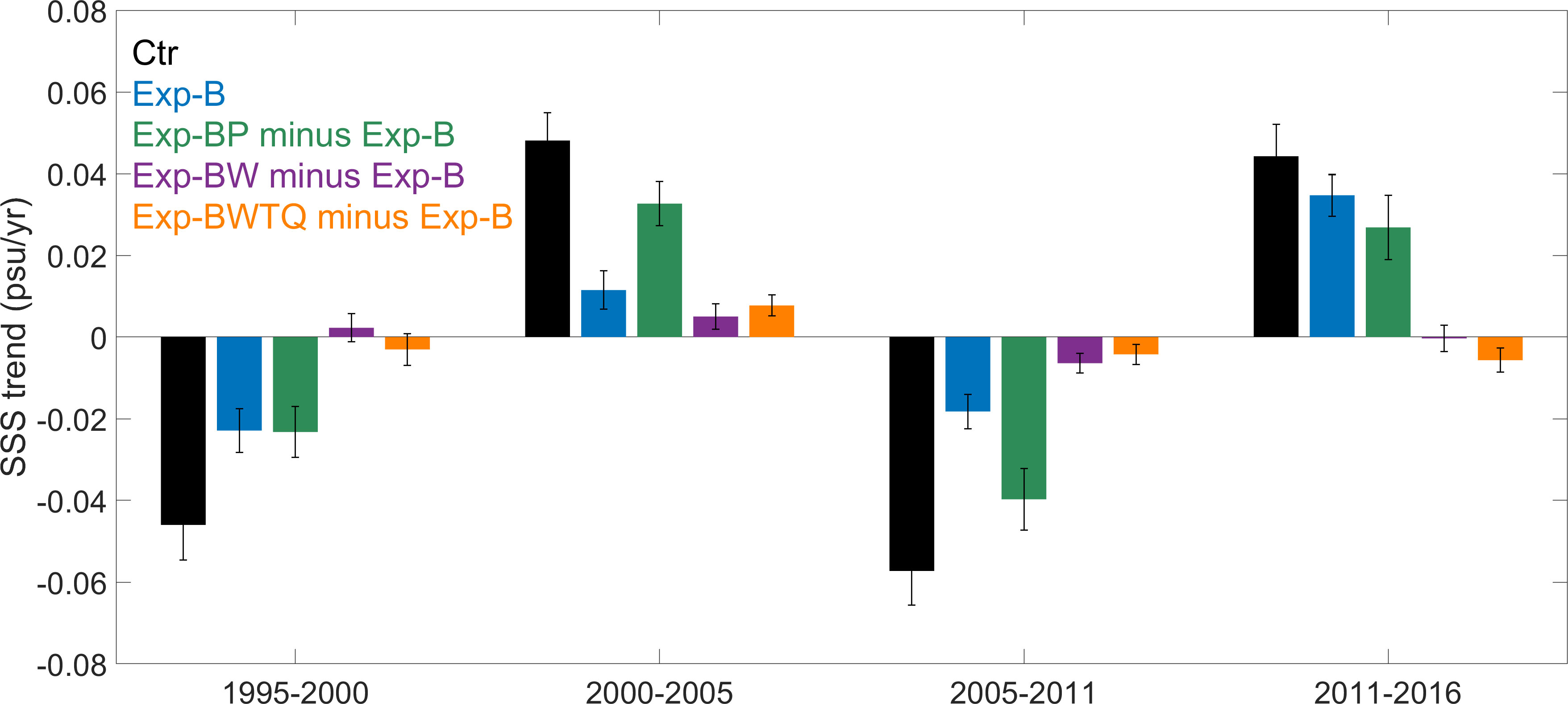
Figure 5 Linear trends of SSS in the SEIO for the periods of 1995-2000, 2000-2005, 2005-2011, and 2011-2016 derived from Ctr (black), Exp-B (blue), Exp-BP minus Exp-B (green) and Exp-BW minus Exp-B (purple), and Exp-BWTQ minus Exp-B (orange). Error-bars denote the 90% confidence interval based on an F test.

We also examined the distributions of SSS changes driven by the ITF and local precipitation (Figure 6). The signatures of the ITF are prominent in its exit area, along the Western Australian coast, and in the 20^o-28^oS band (Figures 6A–D). In contrast, changes forced by precipitation are more widespread, with significant trends extending from the Western Australia coast to the western boundary of the model domain within the entire 10^o-30^oS band (Figures 6E–H). The maximum salinity decrease and increase are about -0.06 psu yr^-1 and +0.05 psu yr^-1, respectively, both greater than those caused by ITF. The result of Exp-BP confirmed that the combined effect of ITF and precipitation explains most of the salinity changes in Ctr, showing the amplitude even stronger than that of Ctr (Figures 6I–L).

FIGURE 6

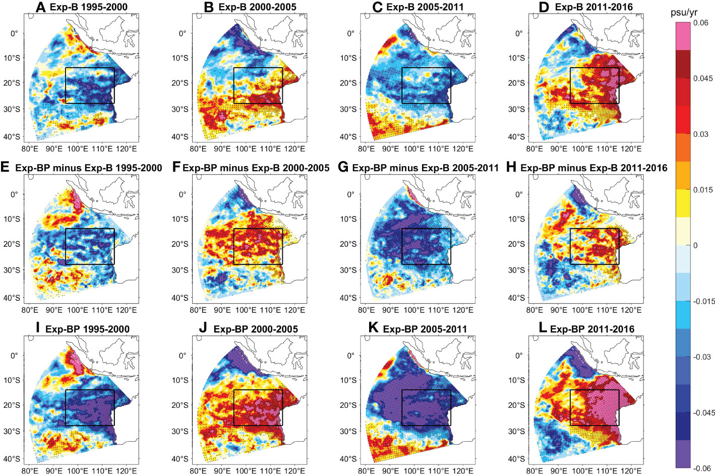
Figure 6 Linear trends maps of SSS derived from Exp-B (A–D), Exp-BP minus Exp-B (E–H), and Exp-BP (I–L) for the periods of 1995-2000, 2000-2005, 2005-2011, and 2011-2016. Stippling indicates significant trends at 90% confidence level based on a Mann-Kendall test. Black lines denote the SEIO region.

4.2. The role of local precipitation

Next, we attempt to understand how local precipitation drives SSS changes in the SEIO. During these four periods, there are large-scale changes of precipitation in the tropical sector of SEIO (north of about 20^oS), showing mainly rainfall increases during 1995-2000 and 2005-2011 and rainfall decreases during 2000-2005 and 2011-2016 (Figure 7). These trends in precipitation are favorable for SSS trends, with enhancing (weakening) precipitation corresponding to the decline (rise) of SSS. However, the center of precipitation changes locates to the north of SSS changes. This can be explained by the transport of ocean surface circulation; the rainfall-driven salinity changes are advected southward by the prevailing southward surface Ekman currents (induced by the southeast trade winds in climatology) in the region (e.g., Wang et al., 2020; Li et al., 2022) and spread to the entire SEIO region.

FIGURE 7

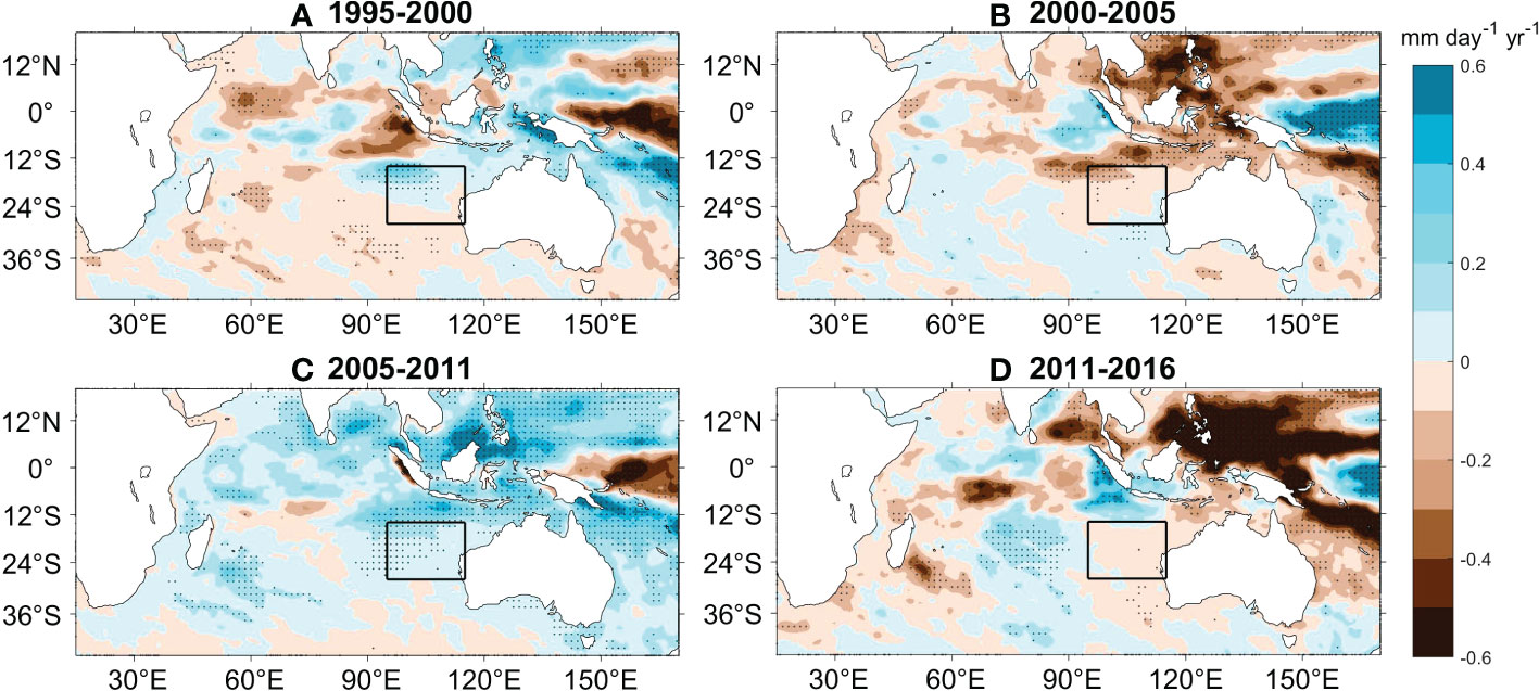
Figure 7 Linear trends of surface precipitation (mm day^-1 year^-1) for the periods of (A) 1995-2000, (B) 2000-2005, (C) 2005-2011, and (D) 2011-2016 derived from ERA-Interim. Stippling indicates significant trends at 90% confidence level based on a Mann-Kendall test. Black lines denote the SEIO.

Figure 8A compares the precipitation rate anomaly and the SSSA of Exp-BP minus Exp-B. The two show clear out-of-phase variations, with positive (negative) SSSAs coinciding with negative (positive) precipitation anomalies. Previous studies have demonstrated that precipitation changes on interannual and decadal timescales in the SEIO region are largely the response to SST variability in the SEIO (e.g., Tozuka et al., 2013; Doi et al., 2015; Li et al., 2019). We further compare the precipitation with the Ningaloo Niño index (NNI) and found a close relationship between the two (correlation coefficient 0.45; Figure 8B). Most of the large precipitation anomalies occur during Ningaloo Niño/Niña events. Therefore, local precipitation changes, which are crucial for SSS changes in this region, are largely generated by local air-sea interaction, with Ningaloo Niño/Niña being the leading mode (e.g., Kataoka et al., 2013; Tozuka et al., 2013; Doi et al., 2015). Note that this relationship also contains influence of interannual variability. The difference between interannual and decadal components will be discussed in the following analysis. The impact of Ningaloo Niño/Niña is further verified by the regression of precipitation anomalies onto NNI (Figure 9). The regression map greatly resembles the observed decadal trends (Figure 7) in spatial pattern, with enhanced rainfall in the tropical sector of the SEIO corresponding to the Ningaloo Niño condition. The regression performed on decadal timescale achieves even larger amplitude in precipitation change (Figure 9B).

FIGURE 8

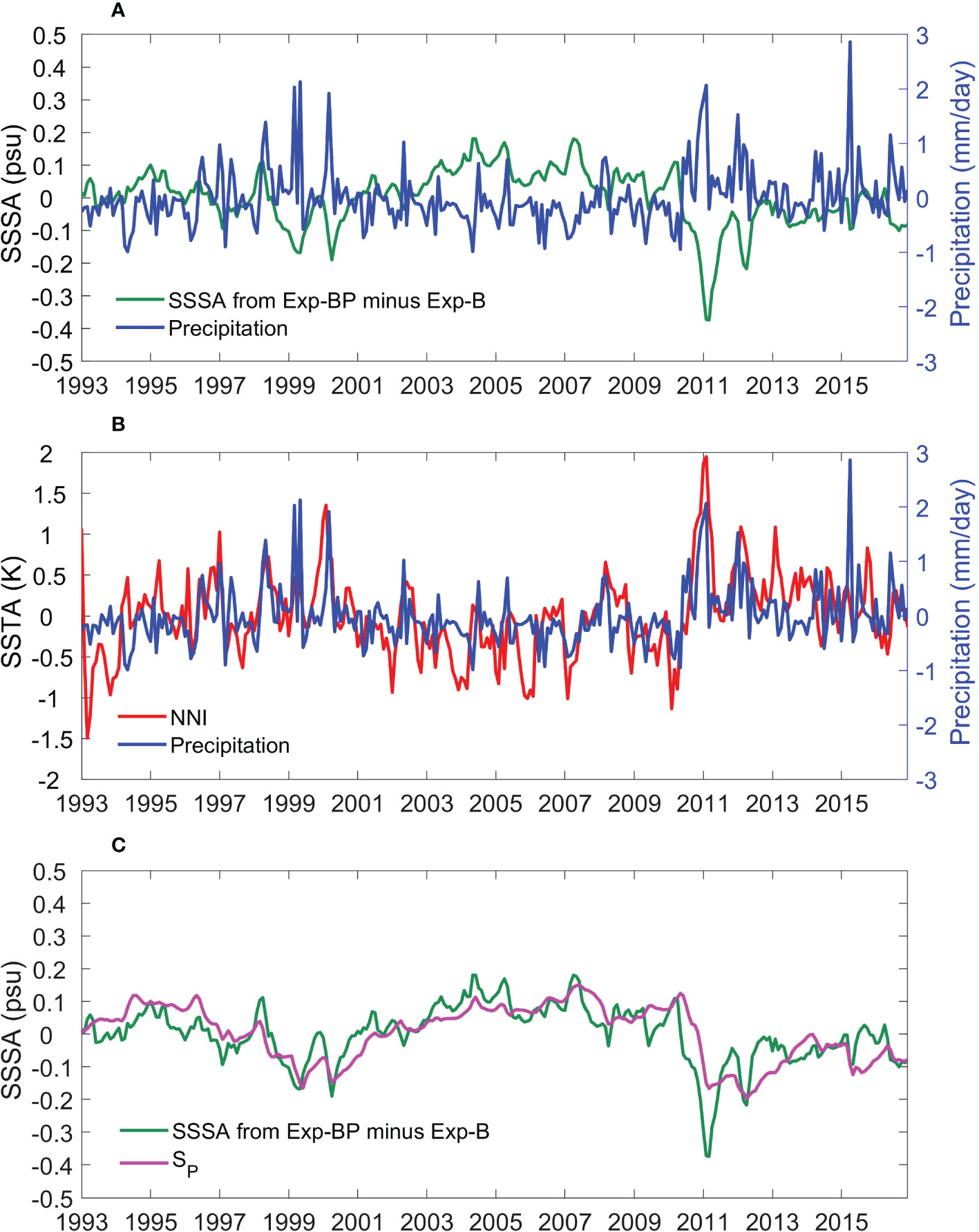
Figure 8 (A) Time series of averaged SSSA (psu) from Exp-BP minus Exp-B and surface precipitation anomalies (mm day^-1) from ERA-Interim for the SEIO region. (B) compares the precipitation anomaly with the Ningaloo Niño index (NNI; in K). NNI is computed as the averaged SST anomaly of the 28^o-22^oS, 108^oE to the coast region (Kataoka et al., 2013). (C) shows the SSSA from Exp-BP minus Exp-B and that simulated by the local rainfall-forced salinity model (LRSM) experiments S_P using ε = 2.75 × 10^-3 s^-1.

FIGURE 9

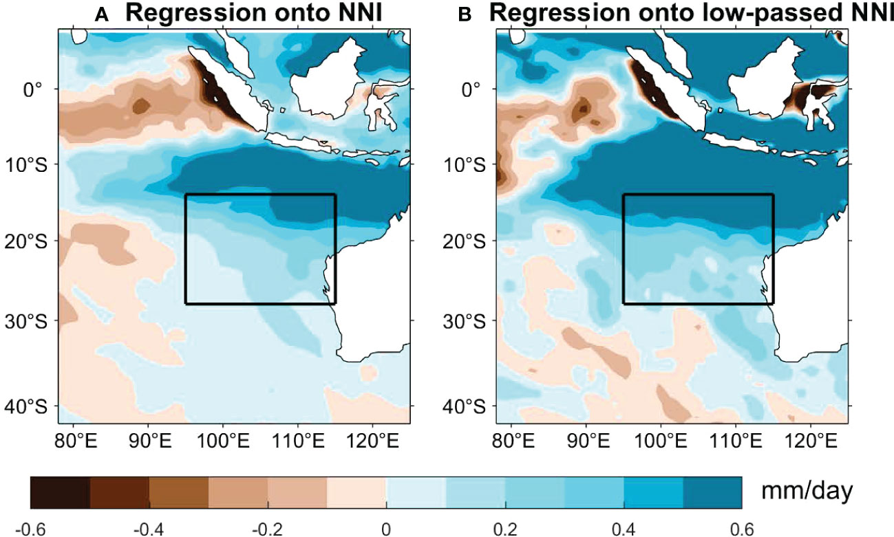
Figure 9 (A) Regression of monthly precipitation anomaly onto NNI. (B) Same as (A) but using 6-year low-passed precipitation and NNI.

Two questions arise from these results. First, the phase lag between precipitation and SSS is not obvious. Their maximum lead-lag correlation is -0.54, when precipitation leads SSS by 1 month. Theoretically, as the forcing and response, precipitation anomaly is supposed to lead the resultant SSSA by about ¹/₄ of the typical period, which is much longer than 1 month. Second, Ningaloo Niño/Niña is primarily an interannual variability mode, with much stronger interannual components than decadal components (Figure 8B). Then, why is the rainfall-forced decadal SSS variability so strong?

To answer the two questions, we devise a simple local rainfall-forced salinity model (LRSM), in which salinity change is governed solely by precipitation anomaly P,

$\begin{array}{ll}\frac{\partial S_P}{\partial t}=-\frac{{\text{S}}_{0}P}{H}-\epsilon S_{\mathrm{P,}}& (1)\end{array}$

where S_P is SSSA, t is time, S₀ = 35.2 psu and H = 30 m are the reference salinity and mixed layer depth, respectively, both obtained from the climatology of ROMS simulation, and ε is the dissipation coefficient. The second term on the right-hand-side, εS_P, represents the damping of S_p by oceanic dynamic processes (e.g., circulation, eddy, and mixing). When only local precipitation produces SSSA, the role of these oceanic dynamic processes is to spread the anomalies elsewhere or to the subsurface ocean, so they generally play a damping role. By assuming the initial S_P on January 1^st 1993 to be zero, S_p is predicted by integrating Equation (1) over time, with P obtained from ERA-Interim data. By changing the value of ε, LRSM achieves good agreement with Exp-BP minus Exp-B at ε = 2.75 x 10^-3 s^-1 (Figures 8C, 10).

FIGURE 10

Figure 10 Results of LRSM simulations as functions of ε varying from 0 to 0.01 s^-1. (A) The correlation coefficient between the SSSA from Exp-BP minus Exp-B and those from by LRSM. (B) The standard deviation of S_p. (C) The time lag (in month) of decadal (6-year low-passed S_p) to decadal precipitation as the function of ε, obtained through a lead-lag correlation analysis. (D) The response efficiency of salinity to precipitation (psu day mm^-1), calculated as the ratio of standard deviation of S_p to that of P. Blue and green lines show the results for interannual variability (6-year high-passed) and decadal variability, respectively. In all panels, ε = 2.75 × 10^-3 s^-1 and corresponding results are marked with dashed lines.

We find that the lag time between precipitation and SSS depends on ε in LRSM. Without the damping effect, that is, ε = 0, S_P is much stronger than ROMS simulation (Exp-BP minus Exp-B), with a standard deviation of 0.19 psu, and the correlation with ROMS simulation is merely r = 0.04 (Figures 10A, B). This inconsistency indicates that even in the rainfall-dominant simulation, ocean dynamics is still essential. At ε = 0, the lag time between S_P and P is 46 months (Figure 10C). As ε increases, S_P gradually decreases in amplitude, and its correlation with ROMS simulation increases. Meanwhile, the lag time between S_P and P is shortened by the increased ε. This is because an anomaly generated early is subjected to a longer dissipation time, and therefore its signature retained in the present S_P (t) is small. As such, the increased dissipation tends to raise the proportion of the newly generated S_p in the present S_P (t) and thereby shortens the lag time between S_P and P. This indicates that the damping effect by ocean dynamics modifies the relationship between precipitation and SSS so that there is no evident phase lag between them.

It should be noted here that even if ε is increased to 0.01 s^-1, the correlation between LRSM and ROMS remains <0.82, and the lag time between S_P and P on decadal time scale is ~4 months, longer than ~1 month lag in the ROMS result. This lag time is still much shorter than the typical lead/lag time of decadal variability, given the ~13-year period of the variability discussed here. Meanwhile, the standard deviation of S_P has been reduced to<0.04 psu. This reflects the limitation of the LRSM model, particularly the simplified representation ocean dynamics. Nevertheless, these LRSM experiments are helpful in understanding how SSS responds to local precipitation change.

We fix ε = 2.75 x 10^-3 s^-1 to examine responses of salinity to precipitation variations on interannual and decadal timescales, respectively. Specifically, we use interannual and decadal components of precipitation, represented by the 6-year high-passed and low-passed for integration precipitation anomalies (Figures 11A, B), in two LRSM integrations, respectively. It is obvious that the interannual precipitation is larger in amplitude than the decadal precipitation. As expected, the S_P produced by interannual precipitation shows mainly interannual variability with very limited decadal variations (Figure 11C), while the S_P produced by decadal precipitation shows strong decadal variations and a correlation of -0.78 with the low-passed NNI (Figure 11D). This confirms that decadal variations in precipitation, which are associated with decadal modulations of Ningaloo Niño/Niña (Feng et al., 2015; Li et al., 2019), give rise to decadal SSS variability in the SEIO. The Ningaloo Niño-like condition of the SEIO enhances local precipitation and cause a decrease in SSS.

FIGURE 11

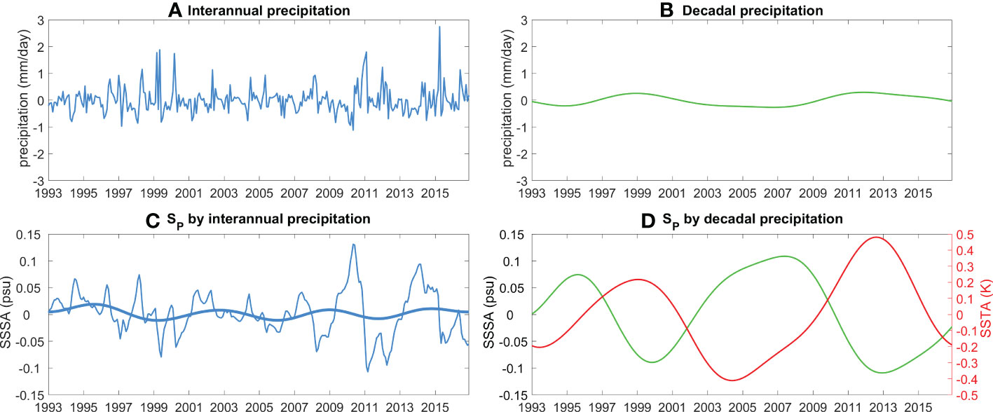
Figure 11 (A) interannual and (B) decadal precipitation variations (mm day^-1) from ERA-Interim over the SEIO region, represented by the 6-year high-pass filtered (blue) and 6-year low-pass filtered (green) precipitation anomalies, respectively. (C, D) show S_p from LRSM experiments forced by interannual and decadal precipitation anomalies, respectively. The thick curve in (C) denotes the 6-year low-passed S_p. The red curve in (D) denotes the NNI (in K).

Note that the amplitude of S_P produced by decadal precipitation (Figure 11D) is no weaker than that produced by interannual precipitation (Figure 11C). This suggests that ocean salinity responds more efficiently to decadal precipitation than to interannual precipitation. We can measure this response efficiency with the ratio of the S_P standard deviation to the P standard deviation, that is, s.d. (S_P)/s.d. (P). At ε = 2.75 x 10^-3 s^-1, the response efficiency on decadal timescale is four-fold larger than that on interannual timescale (Figure 10D). This can be understood as follows. The typical period of precipitation variability is T, and we assume the sine function form,

$\begin{array}{ll}P \left(t\right)=P_0\text{sin}\left(\frac{2\pi }{T}t\right),& (2)\end{array}$

where P₀ is the amplitude of the precipitation. In the case of ε = 0, the salinity anomaly S_P driven by precipitation change can be obtained by integrating Eq. (1),

$\begin{array}{ll}{S}_P \left(t\right)=\frac{S_0{P}_{0}T}{2\pi H}\text{cos}\left(\frac{2\pi }{T}t\right).& (3)\end{array}$

In the above, the amplitude $$\frac{S_0{P}_{0}T}{2\pi H}$$ is proportional to the period T. This explains why the weak decadal precipitation drive strong SSS variability (Figures 11). In our LRSM, the response efficiency also depends on ε. As ε increases, the response efficiency decreases (Figures 10D). Decadal variability is more sensitive to ε than interannual variability. Enhanced damping tends to reduce the dependence of response efficiency on the timescale.

4.3. The role of ITF

In this subsection, we attempt to understand the effect of ITF. The salinity advection by the ITF is determined by two factors, the intensity of the ITF velocities (or volume transport) and the salinity of the ITF water. In our ROMS simulation, both the volume transport and the surface salinity of the ITF show interannual and decadal variations at northeastern boundary of the model domain (Figure 12). The decadal changes of the ITF transport are complicated by strong interannual and shorter-timescale fluctuations, and its relationship with the SEIO salinity is generally not obvious (Figure 12A). One discernible feature is the weakening of the ITF since 2011, which contributes to the SSS salinity increase. By contrast, the ITF’s surface salinity shows clear decadal variations, in agreement with those in the SEIO SSS (Figure 12B). Decadal variability of the ITF and its salinity have been primarily attributed to the tropical Pacific climate (e.g., Du et al., 2015; Feng et al., 2015; Li et al., 2017; Li et al., 2018), as represented by the IPO index (Figure 12C). Processes underlying this linkage are beyond the scope of the present study.

FIGURE 12

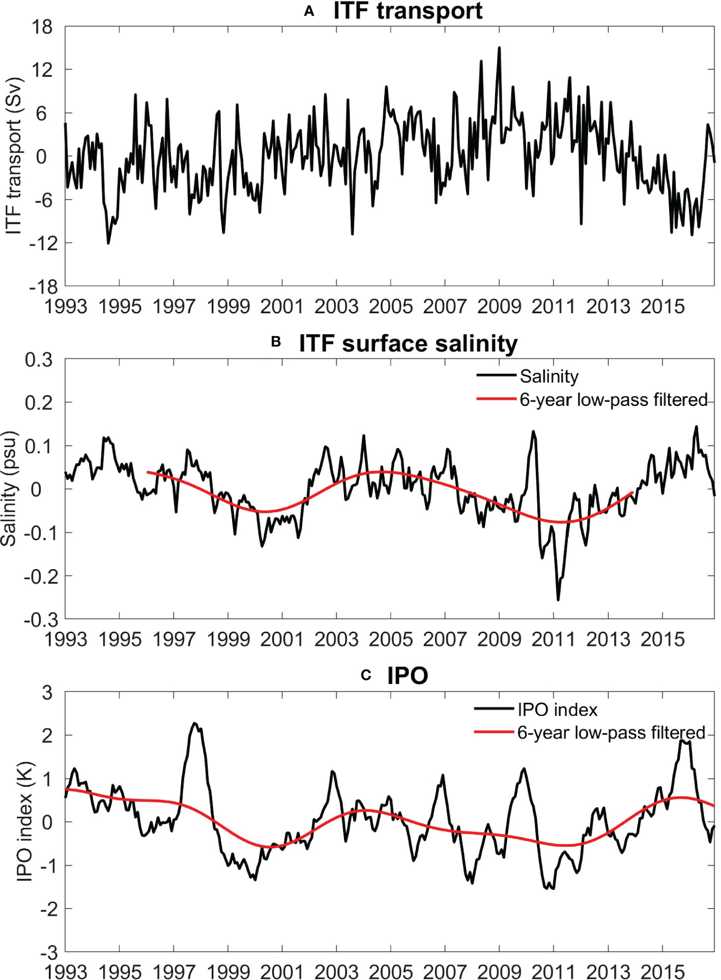
Figure 12 (A) The volume transport of the upper 700 m and (B) the 0-100 m average salinity of the ITF at the northeast boundary of the model domain, derived from Ctr. (C) The IPO index. The 6-year low-passed time series (red) are also shown in (B, C).

To determine the relative importance of the two, we compared the results of Exp-B (including the effect of both factors) and Exp-Bv (including only the effect of ITF intensity). In Exp-Bv, the salinities of the lateral boundary conditions are fixed to climatology, and therefore the ITF affects the SEIO salinity only through its velocities (“v”), while Exp-B minus Exp-Bv represents the influence of the ITF water salinity change. Both can produce strong salinity changes in SEIO (Figure 13). In the two periods of 1995-2000 and 2011-2016, the contributions of the two were approximately equal, while during 2000-2011, the trend in Exp-Bv was larger than that in Exp-B minus Exp-Bv. Overall, both the ITF’s intensity and water salinity are important in causing SSS changes in the SEIO. Under the La Niña-like condition of the tropical Pacific and Ningaloo Niño-like condition of the SEIO (the two often co-occur; Feng et al., 2015; Zhang and Han, 2018; Li et al., 2019), the ITF is enhanced in volume transport and its surface water is freshened by enhanced rainfall over the Indonesian Seas (Du et al., 2015; see also Figure 7). As such, the ITF leads to surface freshening of the SEIO through enhanced transport of fresher than normal water.

FIGURE 13

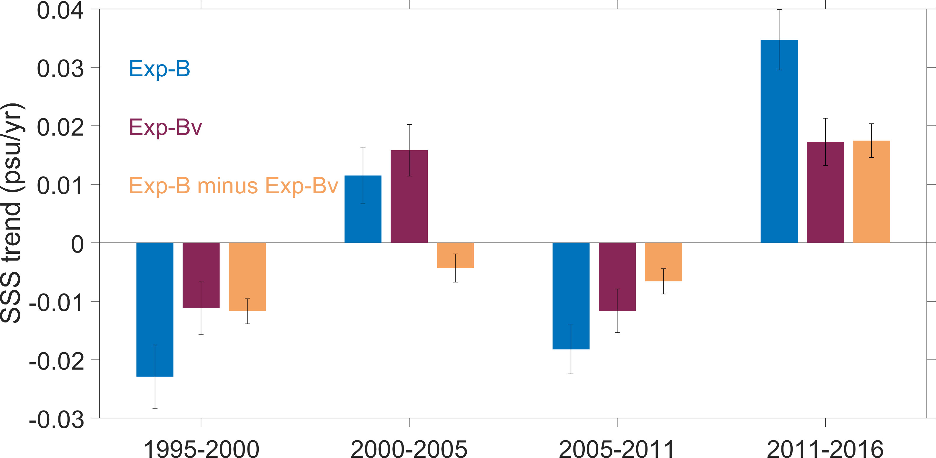
Figure 13 Linear trends of SSS in the SEIO for the periods of 1995-2000, 2000-2005, 2005-2011, and 2011-2016 derived from Exp-B (blue), Exp-Bv (purple) and Exp-B minus Exp-Bv (orange). Error-bars denote the 90% confidence interval based on an F test.

We further present a composite of the SSS-increasing period (averaged from 2000-2005 and 2011-2016) minus the SSS-decreasing period (average of 1995-2000 and 2005-2011) (Figure 14). The weakened ITF intensity mainly caused SSS rise between 15^o-30^oS (Figure 14A). Meanwhile, the increase in the ITF salinity mainly affects its exit area, that is, near the northeast boundary of the model domain. This largely reflects the spreading of salinity changes from the ITF through the mean circulation. By contrast, the salinity increase caused by local winds (Exp-BW minus Exp-B) is quite weak (Figure 14C).

FIGURE 14

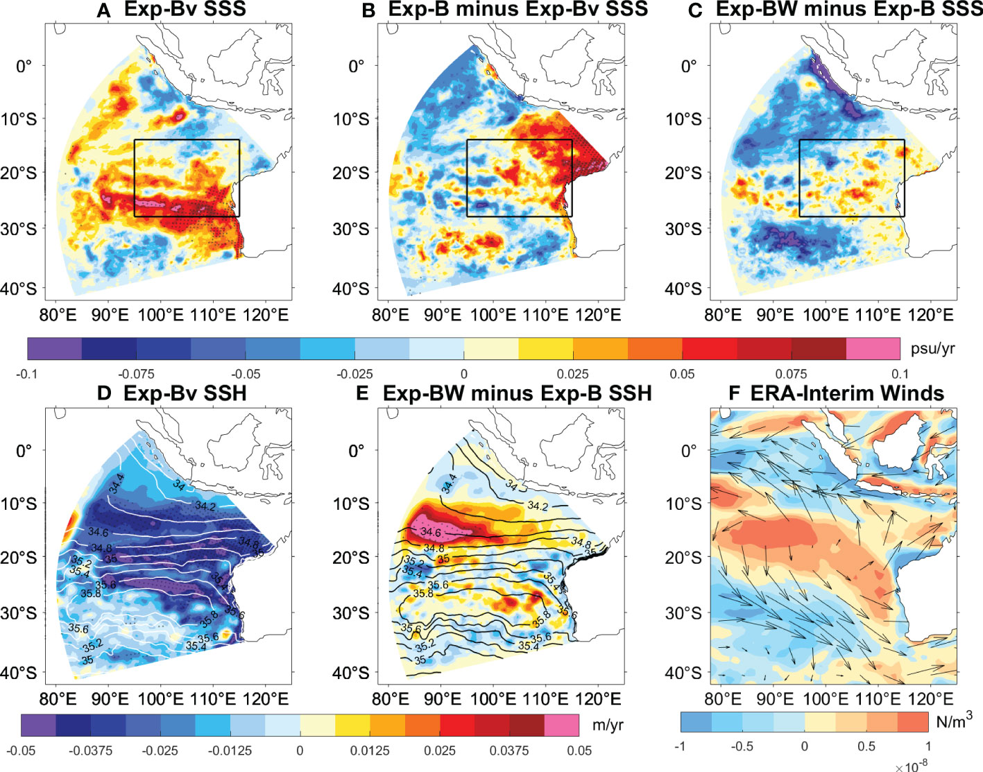
Figure 14 (A) Linear trends maps of SSS derived from Exp-Bv for the composite of 2000-2005 and 2011-2016 minus that of 1995-2000 and 2005-2011. (B, C) As in (A), but for Exp-B minus Exp-Bv and Exp-BW minus Exp-B, respectively. (D) Linear trends maps of SSH derived from Exp-B for the composite of 2000-2005 and 2011-2016 minus that of 1995-2000 and 2005-2011. (E) As in (D), but for Exp-BW minus Exp-B. (D, E) The contour lines represent the climatic salinity of the Ctr data from 1995 to 2016. (F) Linear trends maps of wind stress curl anomaly (shaded) and wind anomaly (vector) derived from ERA-Interim for the composite of 2000-2005 and 2011-2016 minus that of 1995-2000 and 2005-2011. Stippling indicates significant at 90% confidence level based on a Mann-Kendall test. Black lines denote the SEIO.

Sea surface height (SSH) provide useful hints for understanding of the role of these processes. Weakening of ITF transport leads to SSH falling over the SEIO (Feng et al., 2010; Feng et al., 2015; Li et al., 2017), especially at the salinity front between 15^o-30^oS (Figure 14D). The SEIO is governed by the southeasterly trade winds in climatology, and the southward Ekman transport carries low-latitude low-salt water to the south, forming a convergence in the subtropical sector (Wang et al., 2020; Li et al., 2022). This process acts to reduce the SEIO SSS, while the excessive evaporation in the region acts to raise SSS. The decline of SSH represents a divergence in the upper ocean, hindering the southward intrusion of fresh water, thereby causing the SSS rise. The SSH change in Exp-B minus Exp-Bv is quite small (figure not shown).

Local winds cause a weak SSH falling between 20^o-28^oS (Figure 14E), and the corresponding SSS rise there is also limited (Figure 14C). Yet, local winds lead to strong SSH rising between 10^o-20^oS in the SEC region, particularly west of 100^oE. This convergence enhances the southward intrusion of low-latitude fresh water into the region, leading to a decline in SSS. The SSH rise in this region is mainly caused by upwelling Rossby waves excited by the anomalous anticyclonic winds (Figure 14F) via Ekman pumping (Li et al., 2022).

To further illustrate the roles of ITF and local winds, we examined sea surface freshwater flux (E - P) in each experiment (figure not shown). The change in freshwater flux in Exp-B is at least one order of magnitude smaller than that in Exp-BP minus Exp-B and therefore has a very weak effect on salinity. This further confirms that the ITF affects the SEIO salinity mainly through ocean dynamics (such as advection). The change in freshwater flux in Exp-BW minus Exp-B is sizable in magnitude, and it mainly represents wind-controlled evaporation rate. However, this effect is overall out-of-phase with precipitation-dominated freshwater flux, although the correlation is insignificant (-0.09). As such, local winds cannot contribute positively to SSS change through evaporation.

To confirm the roles of ITF and winds through ocean advection, we calculated the advection term for each experiment,

$\begin{array}{ll}\text{ADV}=-u\frac{\partial \text{SSS}}{\partial x}-v\frac{\partial \text{SSS}}{\partial \text{y}}& (4)\end{array}$

where u and v are zonal and meridional surface currents, respectively. In both Exp-B and Exp-Bv experiments, the correlation between ADV and SSS tendency reaches 0.66 (Figures 15A, B), and the amplitude of ADV is larger than SSS tendency. Most of the large SSS tendency anomalies correspond to ADV anomalies. This confirms that changes in the ITF transport can alter the local ocean circulation of SEIO, which in turn induces SSS changes through advection. The ITF water salinity can also cause strong ADV anomalies (Figure 15C), which mainly reflects the spreading of the salinity anomaly at the ITF boundary to the SEIO, but its correlation with SSS tendency is reduced to 0.37. In Exp-BW minus Exp-B, the correlation between SSS tendency and ADV is only 0.07 (Figure 15D). Although local winds can cause strong salinity advection (Huang et al., 2020; Wu et al., 2021), ADV has a weak control effect on SSS. It is possible that the evaporation change and advection driven by winds do not form a synergistic effect or even cancel each other, reducing the overall contribution of local winds to salinity change.

FIGURE 15

Figure 15 Time series of monthly SSS tendency (black; in psu/s) and ADV (red; in psu/s) averaged over the SEIO derived from (A) Exp-B, (B) Exp-Bv, (C) Exp-B minus Exp-Bv and (D) Exp-BW minus Exp-B.

5. Summary and discussion

The SEIO exhibits prominent decadal variability in SSS, with notable impacts on ocean stratification, sea level, and regional circulation. There still lacks a consensus among existing studies on the underlying mechanism. In this study, the ROMS high-resolution model is used to simulate the SSS variability of the SEIO, and a series of sensitivity experiments are used to evaluate contributions of different processes. The findings are summarized as follows.

1) Analysis of observational data suggests that the SEIO showed SSS decreases during 1995-2000 and 2005-2011 and SSS increases during 2000-2005 and post-2011 periods. These decadal changes are faithfully reproduced by ROMS simulation.

2) Through a series of sensitivity experiments, we find that the ITF and local precipitation are major drivers of decadal SSS variability, and the overall contribution of local precipitation is larger. In comparison, local winds and evaporation play minor roles.

3) Further analysis suggests that the phase lag between precipitation anomaly and its resultant SSSA is merely ~1 month, much shorter than expected. Through experiments of the LRSM, we find that oceanic dynamics modify the relationship between precipitation and SSS, greatly shortening their phase lag time. Precipitation change in the SEIO is mainly associated to the decadal variations of Ningaloo Niño/Niña. The response efficiency of salinity to decadal precipitation is significantly higher than that to interannual precipitation.

4) Both the intensity and water salinity of the ITF can drive SSS changes in the SEIO through advection, and their contributions are approximately equal. The ITF intensity change causes large-scale SSS anomalies between 15^o-30^oS, while the ITF salinity change mainly affects its exit area. Although local winds can also cause strong advection, its effect on SSS is small.

The conclusions drawn from our results over the mechanism likely differs from those of existing studies. Salinity budget analysis for the SEIO region indicates that the ocean advection term likely plays a more important role than the surface freshwater forcing term in causing decadal SSS changes (Huang et al., 2020; Wu et al., 2021), while our ROMS experiments suggest the leading role of precipitation. This can be largely reconciled by considering the differences in methodology. In fact, the ocean advection term in the salt budget of a specific box region (such as the SEIO box) has already contained the contribution of precipitation. For example, the SSS anomalies generated north of the SEIO box by precipitation changes (Figure 7) can access the SEIO box via the southward Ekman flows. This part of precipitation-driven change is attributed to advection rather than surface freshwater forcing in budget analysis. With this regard, results based on model sensitivity experiments can better clarify the source of SSS variability.

Simulations in this study were performed using a forced ocean model, which cannot provide insights into the ocean-atmosphere interactions. Nevertheless, the Ctr of ROMS has well reproduced the observed of SSSA in both amplitude and spatial-temporal characteristics, placing confidence for our conclusions. Another issue worthy of discussion is the nonlinearity. Our model experiment design overall adopts the linear assumption, potentially leading to underestimate or overestimate the contribution of a nonlinear process, such as evaporation. Our results indicate that this effect is generally small, given that the sum of individual processes close to the total change. Our simulation stops in December 2016, while Argo data suggest a continued SSS increase till 2020. Whether this trend has reversed during the “multi-year” La Niña condition of 2020-2022 is unknown. This issue will be explored with extended observational data and model simulation, which may provide further insights into the SEIO salinity variability on decadal timescales.

Data availability statement

Publicly available datasets were analyzed in this study. This data can be found here: ERA-Interim data are downloaded from ECMWF interface website https://apps.ecmwf.int/datasets/. Argo and IAP data are available from http://apdrc.soest.hawaii.edu/dods/public_data/Argo_Products and http://159.226.119.60/cheng/, respectively. ROMS simulation is available at Marine Science Data Center, Chinese Academy of Sciences through http://english.casodc.com/data/metadata-special-detail?id=1411169633095917570.

Author contributions

JL performed the analysis and drafted the manuscript. YL proposed and conceived the study and contributed to the paper writing. YG performed the ROMS simulations and contributed to the paper writing. GL and FW contributed to the discussion and paper writing. All authors contributed to the article and approved the submitted version.

Funding

This study is supported by the Laoshan Laboratory (LSKJ202202601), the National Key R&D Program of China (2019YFA0606702), the Strategic Priority Research Program of Chinese Academy of Sciences (XDB42000000), the Shandong Provincial Natural Science Foundation (ZR2020JQ17), and the Project founded by China Postdoctoral Science Foundation (2022M723182).

Acknowledgments

We thank two reviewers for providing insightful comments. ROMS simulations are performed on the Tian-He supercomputer of National Super Computing Center. Discussions with Jing Duan, Mingkun Lv, and Ying Lu are very helpful for this work.

Conflict of interest

The authors declare that the research was conducted in the absence of any commercial or financial relationships that could be construed as a potential conflict of interest.

Publisher’s note

All claims expressed in this article are solely those of the authors and do not necessarily represent those of their affiliated organizations, or those of the publisher, the editors and the reviewers. Any product that may be evaluated in this article, or claim that may be made by its manufacturer, is not guaranteed or endorsed by the publisher.

References

Cheng L., Trenberth K. E., Fasullo J., Boyer T. P., Abraham J., Zhu J. (2017). Improved estimates of ocean heat content from 1960 to 2015. Sci. Adv. 3, e1601545c. doi: 10.1126/sciadv.1601545

CrossRef Full Text | Google Scholar

Cheng L., Trenberth K. E., Gruber N., Abraham J. P., Fasullo J. T., Li G., et al. (2020). Improved estimates of changes in upper ocean salinity and the hydrological cycle. J. Clim. 33 (23), 10357–10381. doi: 10.1175/JCLI-D-20-0366.1

CrossRef Full Text | Google Scholar

Cummings J. (2006). Operational multivariate ocean data assimilation. Q. J. R. Meteorol. Soc. 131, 23. doi: 10.1256/qj.05.105

CrossRef Full Text | Google Scholar

Dee D., Uppala S. M., Simmons A., Berrisford P., Poli P., Kobayashi S., et al. (2011). The ERA-interim reanalysis: Configuration and performance of the data assimilation system. Q. J. R. Meteorol. Soc. 137 (656), 553–597. doi: 10.1002/qj.828

CrossRef Full Text | Google Scholar

Delcroix T., Cravatte S., McPhaden M. J. (2007). Decadal variations and trends in tropical pacific sea surface salinity since 1970. J. Geophys. Res. 112, C03012. doi: 10.1029/2006JC003801

CrossRef Full Text | Google Scholar

Doi T., Behera S., Yamagata T. (2015). An interdecadal regime shift in rainfall predictability related to the ningaloo niño in the late 1990s. J. Geophys. Res. Ocean. 120, 1388–1396. doi: 10.1002/2014JC010562

CrossRef Full Text | Google Scholar

Durack P. J. (2015). Ocean salinity and the global water cycle. Oceanogr. 28, 20–31. doi: 10.5670/oceanog.2015.03

CrossRef Full Text | Google Scholar

Durack P. J., Wijffels S. E., Matear R. J. (2012). Ocean salinities reveal strong global water cycle intensification during 1950 to 2000. Sci 336, 455–458. doi: 10.1126/science.1212222

CrossRef Full Text | Google Scholar

Du Y., Zhang Y., Feng M., Wang T., Zhang N., Wijffels S. (2015). Decadal trends of the upper ocean salinity in the tropical indo-pacificsince mid-1990s. Sci. Rep. 5, 16050. doi: 10.1038/srep16050

PubMed Abstract | CrossRef Full Text | Google Scholar

England M. H., McGregor S., Spence P., Meehl G. A., Timmermann A., Cai W., et al. (2014). Recent intensification of wind-driven circulation in the pacific and the ongoing warming hiatus. Nat. Climate Change 4 (3), 222–227. doi: 10.1038/nclimate2106

CrossRef Full Text | Google Scholar

Feng M., Benthuysen J., Zhang N., Slawinski D. (2015). Freshening anomalies in the Indonesian throughflow and impacts on the leeuwin current during 2010-2011. Geophys. Res. Lett. 42, 8555–8562. doi: 10.1002/2015GL065848

CrossRef Full Text | Google Scholar

Feng M., Majewski L. J., Fandry C., Waite A. M. (2007). Characteristics of two counter-rotating eddies in the leeuwin current system off the Western Australian coast. Deep Res. Part II 54 (8), 961–980. doi: 10.1016/j.dsr2.2006.11.022

CrossRef Full Text | Google Scholar

Feng M., McPhaden M., Lee T. (2010). Decadal variability of the pacific subtropical cells and their influence on the southeast Indian ocean. Geophys. Res. Lett. 37, L09606. doi: 10.1029/2010GL042796

CrossRef Full Text | Google Scholar

Feng M., Wijffels S. E., Godfrey S., Meyers G. (2005). Do eddies play a role in the momentum balance of the leeuwin current? J. Phys. Oceanogr. 35 (6), 964–975. doi: 10.1175/JPO2730.1

CrossRef Full Text | Google Scholar

Guo Y., Li Y., Wang F., Wei Y. (2021). Ocean salinity aspects of the ningaloo niño. J. Clim. 34 (15), 6141–6161. doi: 10.1175/JCLI-D-20-0890.1

CrossRef Full Text | Google Scholar

Guo Y., Li Y., Wang F., Wei Y., Rong Z. (2020a). Processes controlling sea surface temperature variability of ningaloo niño. J. Clim. 33, 4369–4389. doi: 10.1175/JCLI-D-19-0698.1

CrossRef Full Text | Google Scholar

Guo Y., Li Y., Wang F., Wei Y., Xia Q. (2020b). Importance of resolving mesoscale eddies in the model simulation of ningaloo niño. Geophys. Res. Lett. 47, e2020GL087998. doi: 10.1029/2020GL087998

CrossRef Full Text | Google Scholar

Haidvogel D., Arango H., Hedstrom K., Beckmann A., Malanotte-Rizzoli P., Shchepetkin A. (2000). Model evaluation experiments in the north Atlantic basin: Simulations in nonlinear terrain-following coordinates. Dyn. Atmos. Ocean. 32, 239–281. doi: 10.1016/S0377-0265(00)00049-X

CrossRef Full Text | Google Scholar

Helm K., Bindoff N. L., Church J. A. (2010). Changes in the global hydrological-cycle inferred from ocean salinity. Geophys. Res. Lett. 37, L18701. doi: 10.1029/2010GL044222

CrossRef Full Text | Google Scholar

Henley B. J., Gergis J., Karoly D. J., Power S., Kennedy J., Folland C. K. (2015). A tripole index for the interdecadal pacific oscillation. Clim. Dyn. 45, 3077–3090. doi: 10.1007/s00382-015-2525-1

CrossRef Full Text | Google Scholar

Hosoda S., Suga T., Shikama N., Mizuno K. (2009). Global surface layer salinity change detected by argo and its implication for hydrological cycle intensification. J. Oceanogr. 65, 579–586. doi: 10.1007/s10872-009-0049-1

CrossRef Full Text | Google Scholar

Huang J., Zhuang W., Yan X., Wu Z. (2020). Impacts of the upper-ocean salinity variations on the decadal sea level change in the southeast indian ocean during the argo era. Acta Oceanol. Sin. 39 (7), 1–10. doi: 10.1007/s13131-020-1574-4

CrossRef Full Text | Google Scholar

Hu S., Sprintall J. (2016). Interannual variability of the Indonesian throughflow: The salinity effect. J. Geophys. Res. Ocean. 121 (4), 2596–2615. doi: 10.1002/2015JC011495

CrossRef Full Text | Google Scholar

Hu S., Sprintall J. (2017). Observed strengthening of inter-basin exchange via the Indonesian seas due to rainfall intensification. Geophys. Res. Lett. 44 (3), 1448–1456. doi: 10.1002/2016GL072494

PubMed Abstract | CrossRef Full Text | Google Scholar

Hu S., Zhang Y., Feng M., Du Y., Chai F. (2019). Interannual to decadal variability of upper ocean salinity in the southern Indian ocean and the role of the Indonesian throughflow. J. Clim. 32, 6403–6421. doi: 10.1175/JCLI-D-19-0056.1

CrossRef Full Text | Google Scholar

Jia F., Wu L., Qiu B. (2011). Seasonal modulation of eddy kinetic energy and its formation mechanism in the southeast Indian ocean. J. Phys. Oceanogr. 41 (4), 657–665. doi: 10.1175/2010JPO4436.1

CrossRef Full Text | Google Scholar

Kataoka T., Tozuka T., Behera S., Yamagata T. (2013). On the ningaloo Niño/Niña. Climate Dyn. 43, 1463–1482. doi: 10.1007/s00382-013-1961-z

CrossRef Full Text | Google Scholar

Lebedev K., Yoshinari H., Maximenko N., Hacker P. (2007). Velocity data assessed from trajectories of argo floats at parking level and at the sea surface. IPRC Tech. Note 4 (2). doi: 10.13140/RG.2.2.12820.71041

CrossRef Full Text | Google Scholar

Li G., Cheng L., Zhu J., Trenberth K. E., Mann M. E., Abraham J. P. (2020). Increasing ocean stratification over the past half-century. Nat. Climate Change 10 (12), 1116–1123. doi: 10.1038/s41558-020-00918-2

CrossRef Full Text | Google Scholar

Li Y., Guo Y., Zhu Y., Kido S., Zhang L., Wang F. (2022). Variability of heat content and eddy kinetic energy in the southeast Indian ocean: Roles of the Indonesian throughflow and local wind forcing. J. Phys. Oceanogr. 52 (11), 2789–2806. doi: 10.1175/JPO-D-22-0051.1

CrossRef Full Text | Google Scholar

Li Y., Han W., Hu A., Meehl G. A., Wang F. (2018). Multidecadal changes of the upper Indian ocean heat content during 1965–2016. J. Clim. 31 (19), 7863–7884. doi: 10.1175/JCLI-D-18-0116.1

CrossRef Full Text | Google Scholar

Li Y., Han W., Zhang L. (2017). Enhanced decadal warming of the southeast Indian ocean during the recent global surface warming slowdown. Geophys. Res. Lett. 44, 9876–9884. doi: 10.1002/2017GL075050

CrossRef Full Text | Google Scholar

Li Y., Han W., Zhang L., Wang F. (2019). Decadal SST variability in the southeast Indian ocean and its impact on regional climate. J. Clim. 32, 6299–6318. doi: 10.1175/JCLI-D-19-0180.1

CrossRef Full Text | Google Scholar

Llovel W., Lee T. (2015). Importance and origin of halosteric contribution to sea level change in the southeast Indian ocean during 2005-2013. Geophys. Res. Lett. 42 (4), 1148–1157. doi: 10.1002/2014GL062611

CrossRef Full Text | Google Scholar

Lu Y., Li Y., Duan J., Lin P., Wang F. (2022). Multidecadal Sea level rise in the southeast Indian ocean: The role of ocean salinity change. J. Clim. 35 (5), 1479–1496. doi: 10.1175/JCLI-D-21-0288.1

CrossRef Full Text | Google Scholar

Masson S., Delecluse P., Boulanger J., Menkes C. E. (2002). A model study of the seasonal variability and formation mechanisms of the barrier layer in the eastern equatorial Indian ocean. J. Geophys. Res. 107 (12), 8017. doi: 10.1029/2001JC000832

CrossRef Full Text | Google Scholar

Meehl G. A., Arblaster J. M., Fasullo J. T., Hu A., Trenberth K. E. (2011). Model-based evidence of deep-ocean heat uptake during surface-temperature hiatus periods. Nat. Climate Change 1 (7), 360–364. doi: 10.1038/NCLIMATE1229

CrossRef Full Text | Google Scholar

Menezes V., Phillips H., Schiller A., Domingues C., Bindoff N. (2013). Salinity dominance on the Indian ocean Eastern gyral current. Geophys. Res. Lett. 40 (21), 5716–55721. doi: 10.1002/2013GL057887

CrossRef Full Text | Google Scholar

Nie X., Wei Z., Li Y. (2020). Decadal variability in salinity of the indian ocean subtropical underwater during the argo period. Geophys. Res. Lett. 47, (22). doi: 10.1029/2020GL089104

CrossRef Full Text | Google Scholar

Qu T. D., Meyers G. (2005). Seasonal variation of barrier layer in the southeastern tropical Indian ocean. J. Geophys. Res. 110, C11003. doi: 10.1029/2004JC002816

CrossRef Full Text | Google Scholar

Qu T. D., Meyers G. (2005a). Seasonal characteristics of circulation in the southeastern tropical Indian ocean. J. Phys. Oceanogr. 35, 244–267. doi: 10.1175/JPO-2682.1

CrossRef Full Text | Google Scholar

Rayner N. A. (2003). Global analyses of sea surface temperature, sea ice, and night marine air temperature since the late nineteenth century. J. Geophys. Res. 108, 4407. doi: 10.1029/2002JD002670

CrossRef Full Text | Google Scholar

Saji N. H., Yamagata T. (2003). Structure of SST and surface wind variability during Indian ocean dipole mode events: COADS observations. J. Clim. 16, 2735–2751. doi: 10.1175/1520-0442(2003)016

CrossRef Full Text | Google Scholar

Schmitt R. W. (2008). Salinity and the global water cycle. Oceanography 21, 12–19. doi: 10.5670/oceanog.2008.63

CrossRef Full Text | Google Scholar

Skliris N., Zika J. D., Nurser G., Josey S. A., Marsh R. (2016). Global water cycle amplifying at less than the clausius-clapeyron rate. Sci. Rep. 6, 38752. doi: 10.1038/srep38752

PubMed Abstract | CrossRef Full Text | Google Scholar

Taylor K. E., Stouffer R. J., Meehl G. A. (2012). An overview of CMIP5 and the experiment design. Bull. Am. Meteorol. Soc. 93 (4), 485–498. doi: 10.1175/BAMS-D-11-00094.1

CrossRef Full Text | Google Scholar

Terray L., Corre L., Cravatte S., Delcroix T., Reverdin G., Ribes A. (2012). Near-surface salinity as nature’s rain gauge to detect human influence on the tropical water cycle. J. Clim. 25 (3), 958–977. doi: 10.1175/JCLI-D-10-05025.1

CrossRef Full Text | Google Scholar

Tozuka T., Kataoka T., Yamagata T. (2013). Locally and remotely forced atmospheric circulation anomalies of ningaloo Niño/Niña. Climate Dyn. 43, 2197–2205. doi: 10.1007/s00382-013-2044-x

CrossRef Full Text | Google Scholar

Wang Y., Li Y., Wei C. (2020). Subtropical sea surface salinity maxima in the south Indian ocean. J. Oceanol. Limnol. 38, 16–29. doi: 10.1007/s00343-019-8251-5

CrossRef Full Text | Google Scholar

Wijffels S., Meyers G. (2004). An intersection of oceanic waveguides: Variability in the Indonesian throughflow region. J. Phys. Oceanogr. 34, 1232–1253. doi: 10.1175/1520-0485(2004)034<1232:AIOOWV>2.0.CO;2

CrossRef Full Text | Google Scholar

Wu Y., Zheng X., Sun Q., Zhang Y., Du Y., Liu L. (2021). Decadal variability of the upper ocean salinity in the southeast indian ocean: role of local ocean-atmosphere dynamics. J. Clim. 34 (19), 7927–7942. doi: 10.1175/JCLI-D-21-0122.1

CrossRef Full Text | Google Scholar

Yu L. (2011). A global relationship between the ocean water cycle and near-surface salinity. J. Geophys. Res. 116, C10025. doi: 10.1029/2010JC006937

CrossRef Full Text | Google Scholar

Yu L., Josey S. A., Bingham F. M., Lee T. (2020). Intensification of the global water cycle and evidence from ocean salinity: a synthesis review. Ann. New York Acad. Sci. 1472, 76–94. doi: 10.1111/nyas.14354

CrossRef Full Text | Google Scholar

Zhang Y., Du Y., Feng M. (2017). Multiple time scale variability of the Sea surface salinity dipole mode in the tropical Indian ocean. J. Climate 31 (1), 283–296. doi: 10.1175/JCLI-D-17-0271.1

CrossRef Full Text | Google Scholar

Zhang N., Feng M., Du Y., Lan J., Wijffels S. E. (2016a). Seasonal and interannual variations of mixed layer salinity in the southeast tropical Indian ocean. J. Geophys. Res. Ocean. 121, 4716–4731. doi: 10.1002/2016JC011854

CrossRef Full Text | Google Scholar

Zhang Y., Du Y., Qu T. (2016b). A sea surface salinity dipole mode in the tropical Indian ocean. Climate Dyn. 47, 2573–2585. doi: 10.1007/s00382-016-2984-z

CrossRef Full Text | Google Scholar

Zhang L., Han W. (2018). Impact of ningaloo niño on tropical pacific and an interbasin coupling mechanism. Geophys. Res. Lett. 45, 11300–11309. doi: 10.1029/2018GL078579

CrossRef Full Text | Google Scholar

Zhang L., Han W., Li Y., Shinoda T. (2018). Mechanisms for generation and development of ningaloo niño. J. Clim. 31, 9239–9259. doi: 10.1175/JCLI-D-18-0175.1

CrossRef Full Text | Google Scholar

Zika J. D., Skliris N., Blacker T. A., Marsh R., Nurser A. J. G., Josey S. A. (2018). Improved estimates of water cycle change from ocean salinity: The key role of ocean warming. Environ. Res. Lett. 13, 074036. doi: 10.1088/1748-9326/aace42

CrossRef Full Text | Google Scholar