 Jian Li
 Peiliang Li
 Peng Bai
 Fangguo Zhai
 Yanzhen Gu1,2*
 Wenfan Wu
94% of researchers rate our articles as excellent or good
Learn more about the work of our research integrity team to safeguard the quality of each article we publish.
Find out more
ORIGINAL RESEARCH article
Front. Mar. Sci., 15 December 2022
Sec. Coastal Ocean Processes
Volume 9 - 2022 | https://doi.org/10.3389/fmars.2022.1092984
This article is part of the Research TopicMacroecology of Coastal Zone under Global ChangesView all 15 articles
Coastal fronts play vital roles in local biogeochemical environment. An abrupt change of Zhejiang-Fujian coastal front (ZFCF) during early spring was well captured by multi-source satellite-retrieved sea surface temperature images. Here in this study, we investigated the mechanism of the abrupt decay with a combination of satellite observation and numerical simulation. Correlation analysis of long-term reanalysis data indicates that the variability of wind, heat flux and the Zhejiang-Fujian coastal current (ZFCC) have significant relationships with the variation of ZFCF in winter. Following heat budget analysis points out that net heat flux and horizontal advection are important in determining the net temperature tendency difference between two water masses of ZFCF during this process. To further explore the intrinsic physical roles of different dynamic factors, a comprehensive numerical investigation was conducted. Compared with the observations, the model reproduced the abrupt change process of the ZFCF satisfyingly. Sensitive experiments reveal that the weakening of the ZFCC, caused by the relaxation of the monsoon, contributes to the abrupt decay of ZFCF in the first half period, and heating effect of the Kuroshio Intrusion (KI) water gives rise to the following half period of the decay under the recovered monsoon. Further, with the impact of the KI water after the change, the ZFCF can be maintained even if the ZFCC is weak, whereas in January, the contribution of the KI water to the formation of the ZFCF seems to be limited under the prevailing monsoon. Besides, the riverine discharge and the tidal forcing can also modulate the spatiotemporal variation of ZFCF, the decrease of the river input also intensifies that decay, while tides fix the front at a specific depth.
Coastal front is a significant hydrodynamic phenomenon located on the boundary between two distinct water masses with remarkably high gradients of temperature, salinity, density, nutrient, or other environmental variables (Cromwell and Reid, 1956; Belkin and O'Reilly, 2009). The frontal process is one of the most important physical processes in the coastal marine environment (McWilliams, 2021), playing a vital role in the regional ecosystem, fishery, and carbon cycling system (Alemany et al., 2014; Lohmann and Belkin, 2014; Androulidakis et al., 2018).
Occurring along the 50-m isobath off the Zhejiang-Fujian coast (Figure 1), the Zhejiang–Fujian coastal front (ZFCF) is known as a major part of the East China Sea (ECS) coastal front system (Hickox et al., 2000), and generally exists as a multi-type front (Chen, 2009; He et al., 2016; Cao et al., 2021). Thus, the ZFCF is closely associated with fish abundance (Huang et al., 2010). For instance, the famous Zhoushan fishing ground is right located around the ZFCF, of which the total fishery production is 1.8 million tons in 2021. Moreover, algal bloom (Zhang et al., 2018) and suspended sediments (Qiao et al., 2020) are also significantly modulated by ZFCF.
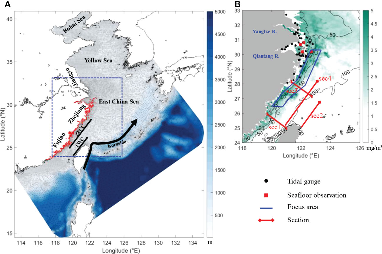
Figure 1 (A) Bathymetry and mesh grid of the studied region, the Zhejiang-Fujian coast is highlighted in the red line. (B) Monthly MODIS-Aqua chlorophyll-a concentration off the Zhejiang-Fujian coast in March, 2021.
Former investigations date back to the 1980s have clarified the spatiotemporal variation of the ZFCF through in-situ observation, satellite remote sensing and numerical modeling. The ZFCF characterizes significant seasonal variability, it appears in autumn, strengthens in winter, and dissipates in summer (Hickox et al., 2000; Huang et al., 2010; He et al., 2016). Based on satellite retrieved sea surface temperature (SST), He et al. (2016) demonstrated that the ZFCF is a double coastal front system consisting of a Zhejiang-Fujian offshore thermal coastal front along the 50-m isobath and a near-shore coastal thermal front along the 20-m isobath, of which the width is about 73.5 km.
Most of previous studies share the same perspective that the Zhejiang-Fujian coastal current (ZFCC) and Taiwan Warm Current (TWC) are two essential factors in modulating the ZFCF (Tseng et al., 2000; Hsieh et al., 2004; Komatsu et al., 2007; Chen, 2009; Bian et al., 2013). Driven by the northeast monsoon, ZFCC usually forms in boreal autumn and winter, travelling southward with fresh, cold and eutrophic water sourced along the eastern Chinese coast. Zhang et al. (2005) pointed out that wind stress is a critical factor controlling the ZFCC’s variation on the diurnal timescale. Through a de-tiding analysis on the ZFCC, Wu et al. (2013) summarized that buoyancy also makes vital contributions to the water transport along local coast. Recently, wind-induced sea level variation and buoyancy forcing from river discharge were reported to make quasi-equivalent contributions in driving ZFCC (Zhang et al., 2022).
The TWC is usually considered as the current originating from Taiwan Strait or Kuroshio Intrusion (KI), flowing toward north all year around within the 50-100m isobaths (Mao, 1964). The TWC significantly impacts the shelf environment and ecosystem of ECS, however, its origin and flow pathway are still controversial. To date, it is widely accepted that in summer, the TWC consists of both the northward flow through Taiwan Strait and the branch of Kuroshio intruding into the ECS. But in winter, no consensus has been reached so far (Isobe, 2008; Lian et al., 2016b). Therefore, impacts of TWC on the ZFCF exerted either by Taiwan Strait warm water or the Kuroshio Current (KC) remains to be elucidated.
Except for the large-scale background circulation, other factors also can modulate the ZFCF. He et al. (2016) indicated that the steep bottom bathymetry off the Zhejiang-Fujian coast and surface cooling jointly contribute to the formation of the ZFCF. Cao et al. (2021) analyzed the relationships between the potential driving forces (e.g., alongshore wind, river discharge and SST) and fronts probability using linear regression method, whose results highlighted the significant roles of alongshore wind and the river discharge in the frontogenesis of ZFCF.
Previous studies have achieved a comprehensive understanding of the ZFCF over a seasonal scale, however, the spatiotemporal variability and regulatory mechanisms of ZFCF over a shorter time scale remain unclear. Using multi-source remote-sensed SST data, a new phenomenon was captured: there is an abrupt change in the intensity of the ZFCF in early spring, 2021, which certainly will exert a significant impact on local coastal ecosystem. In order to explore the intrinsic mechanisms controlling the abrupt change of the ZFCF and achieve a better understanding of local marine environment, a series of numerical investigations together with remote sensing data analysis and heat budget analysis were conducted. Following this introduction, section 2 introduces the remote sensing data, numerical model configuration, and model validations; section 3 presents the three-dimensional structures of the ZFCF and its variability; section 4 documents a systematic discussion of factors controlling the abrupt change of ZFCF, and finally, section 5 summarizes the current study.
Three sources of satellite data were employed in this study, including the Moderate Resolution Imaging Spectroradiometer (MODIS) -Aqua Daytime SST, Multiscale Ultrahigh Resolution (MUR) SST and Himawari-8 SST. The available periods of these data are 2002-07 to ongoing, 2002-06 to ongoing and 2015-06 to ongoing, respectively.
Monthly averaged MODIS -Aqua SST Level 3 Mapped data with a spatial resolution of 4 km × 4 km during 2003 to 2021 were obtained from the U.S. National Aeronautics and Space Administration (NASA) website1. Together with MODIS-Aqua SST, two more datasets were used for comparison and verification. The MURSST Level 4 SST, produced by NASA JPL Physical Oceanography DAAC2 with a 0.01-degree resolution, is based upon nighttime GHRSST L2P skin and subskin SST observations from several instruments, including the AMSR-E, AMSR-2, MODIS, WINDSAT radiometer, AVHRR, and in situ SST observations from the NOAA iQuam project. In this study, daily MURSST data from October 2020 to June 2021 are used. The monthly Level 3 Himawari-8 SST data with a 2 km spatial resolution from October 2020 to June 2021 were provided by the Japan Meteorological Agency (JMA)3, this product is mainly based on the observations by the new generation geostationary satellite Himawari-8. Notably, the Himawari-8 SST has been validated against the in-situ SST data (iQuam) and shows reliable quality.
The seafloor observations are achieved through the submarine cable observation systems (Zhai et al., 2020). These systems were applied to online monitor temporal variations in marine environment of the ecologically important regions. Four submarine cable observation systems are marked off with red squares around the Changjiang and Qiantangjiang estuaries in Figure 1B. The submarine cable online observation systems were placed at 20 cm above the sea floor and equipped with a HydroCAT conductivity-temperature-depth (CTD) recorder to continuously observe temperature, salinity, pressure and other variables in the bottom layer. In this study, hourly averaged temperature in bottom layer and the water elevation were used to examine the performance of the numerical model.
ERA54 is the fifth generation ECMWF reanalysis of the global climate and weather, which provides hourly estimates for a large number of atmospheric, ocean-wave and land-surface quantities. In this study, 0.25-degree hourly wind vectors and surface radiation flux data, including Surface net solar radiation (SNSR), Surface net thermal radiation (SNTR), Surface sensible heat flux (SSHF), and Surface latent heat flux (SLHF), of 2020 to 2021 are used as the atmospheric forcing in our model. Meanwhile, ERA5 data from 2003 to 2021 were also utilized in the correlation analysis in section 4. The ECMWF convention for vertical fluxes is positive downwards, and net heat flux from ERA5 is calculated following:
SST gradient magnitude was calculated by the central difference method as:
Where ∇xSST and ∇ySST are the zonal and meridional components of the SST gradient, ΔX and ΔY are the distances in kilometers between the neighboring grid points in the longitudinal and latitudinal directions, respectively. |∇SST| is the gradient magnitude. This algorithm has been widely used in the calculation of coast SST gradient (Vazquez-Cuervo et al., 2013; Saldias and Lara, 2020; Saldias et al., 2021).
The studied region characterizes irregular coastline and rugged topography, therefore the traditional circulation model working under structured grid is no longer capable. For this reason, the Semi-implicit Cross-scale Hydroscience Integrated System Model (SCHISM) was employed in this study (Zhang et al., 2016a; Zhang et al., 2016b). SCHISM is a 3D unstructured-grid model developed from the original Eulerian-Lagrangian Finite Element model, using the semi-implicit time stepping and hybrid finite-element/finite-volume method with the Eulerian-Lagrangian algorithm to solve the Navier-Stokes equations in hydrostatic form. In addition, it provided a new hybrid SZ coordinate called Localized Sigma Coordinates with Shaved Cells (LSC2) in the vertical dimension, which makes no bathymetry smoothing possible. More details about the SCHISM model can be found on its official website5.
The model region covers the whole Bohai sea, Yellow sea, and East China Sea with three open boundaries (Figure 1A). In order to better simulate the hydrodynamics in the nearshore areas and save computational resources, the locally-refined grid was designed. The horizontal resolution near the open boundaries is depth-dependent varying between 7 to 50 km, while for the refined regions (blue dotted box in Figure 1A), the horizontal resolution ranges from 2 km in the shallow coastal water to 8 km in the deeper area. The whole mesh grid contains 24742 nodes and 47319 triangle elements. In the vertical direction, 59 layers LSC2 grid was applied and the bathymetry was interpolated from the Shuttle Radar Topography Mission (SRTM) 15Plus V2.1 (Tozer et al., 2019).
The 3-D water temperature, salinity, velocity, and sea surface height for initial and boundary conditions were interpolated from the 41-layer Hybrid Coordinate Ocean Model and Navy Coupled Ocean Data Assimilation (HYCOM + NCODA) Global 1/12° Analysis data. Additionally, we prescribed the tidal forcing of eight tidal components, including M2, S2, K2, N2, K1, O1, Q1, and P1 at the open boundaries. All the tidal information comes from the latest version of the Finite Element Solution (FES2014) tide model by AVISO+6. We considered two major river sources, the Yangtze River and the Qiantang River, the monthly averaged river discharge data is from the River and Sediment Bulletin of China7, besides, the temperature of the rivers is based on MODIS-Aqua 4km daily SST product, and the salinity is set to 3 PSU uniformly. Hourly atmospheric forcing was generated using the ERA5 product originated from Climate Data Store4. The simulation period was initialized on October 1, 2020 and ended on December 31, 2021. During the integration, the time step was 120s and hourly outputs were saved.
Figure 2 displays the monthly mean SST gradient magnitude and the 10m-high wind vectors from October, 2020 to March, 2021 within the study area. In November, the ZFCF started to form under the strong prevailing northeast monsoon, then its intensity kept strengthening along the 50-m isobath and peaked in January, with a maximum intensity of 0.2°C/km. In the following February and March, there was a significant decrease in both the intensity and spatial range of the ZFCF, especially in the area south of the 28°N, the SST gradient has dropped by more than 0.12°C/km and the front almost disappeared by March. However, compared with the evolution of winds in January, there is no significant change in the local wind both in speed and direction.
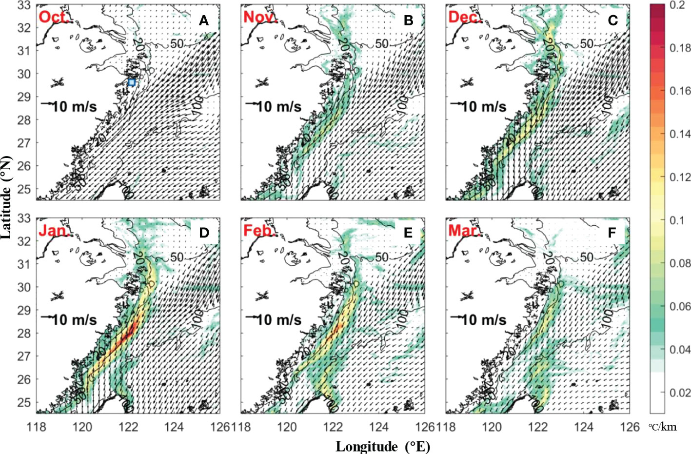
Figure 2 MURSST monthly mean SST gradient magnitude and ERA5 10m wind vectors in the Zhejiang-Fujian coastal sea from October (A) to March (F) of 2020-2021.
To show this phenomenon in more detail, we calculated the time series of spatially-averaged daily SST gradient as well as the local wind vectors of the focus region (blue dashed box in Figure 1A) and presented them in Figure 3. As revealed by Figure 3, when entering January, the SST gradient shows a high correlation with the southward meridional wind, e.g., it increases significantly during these two strong northerly wind processes around early January and mid-February, respectively, which agrees with the points of previous works (Cao et al., 2021). Then an abnormal abrupt decrease of the SST gradient occurred: the magnitude of SST gradient in the focus region quickly dropped by more than 0.05 °C/km during 15 days after late January, which is highlighted in red in Figure 3. This phenomenon can be divided into two periods: in the first period, the northerly wind significantly weakens and there is a synchronous dramatic decrease in SST gradient; in the second period, after the recovery of the northerly monsoon, the SST gradient does not recover as expected but oppositely a repaid decline process occurs. So, how does this phenomenon develop?
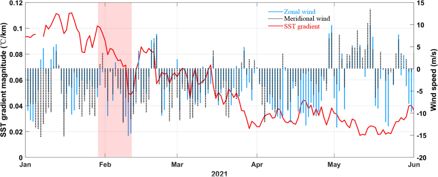
Figure 3 The spatially-averaged SST gradient magnitude of the focus region (Figure 1B) is shown in the red line, while the speed of zonal and meridional wind from ERA5 is in the blue line and black-dots-line (eastward and northward positive), respectively. The red shaded region marks off the sudden decrease of the SST gradient.
The satellite observed SST has captured the rapid changes of the ZFCF successfully, however, it is hard to further investigate the regulatory mechanism of this phenomenon, thus the numerical model is employed to make further explorations. To ensure the reliability of the discussions, we first validated the model performance in describing local hydrodynamics.
Previous studies indicated that tides make significant contributions to the hydrodynamic field in ECS by generating internal solitary waves, tidal fronts and other processes (Hu et al., 2016; Teng et al., 2017; Liu et al., 2018; Wang et al., 2020). So, we first compared the simulated hourly sea elevation against the observations from the submarine cable observation system in January (Figure 4). As displayed, the model well reproduced the time series of elevation at stations Dajishan and Dongjidao 1 only with minor differences. To further evaluate the performance of the model, we calculate three statistical parameters, including Root Mean Square Error (RMSE), Correlation Coefficient (CC) and model Skill, and the model skill assessment parameter is defined as (Bai et al., 2016; Lai et al., 2018):
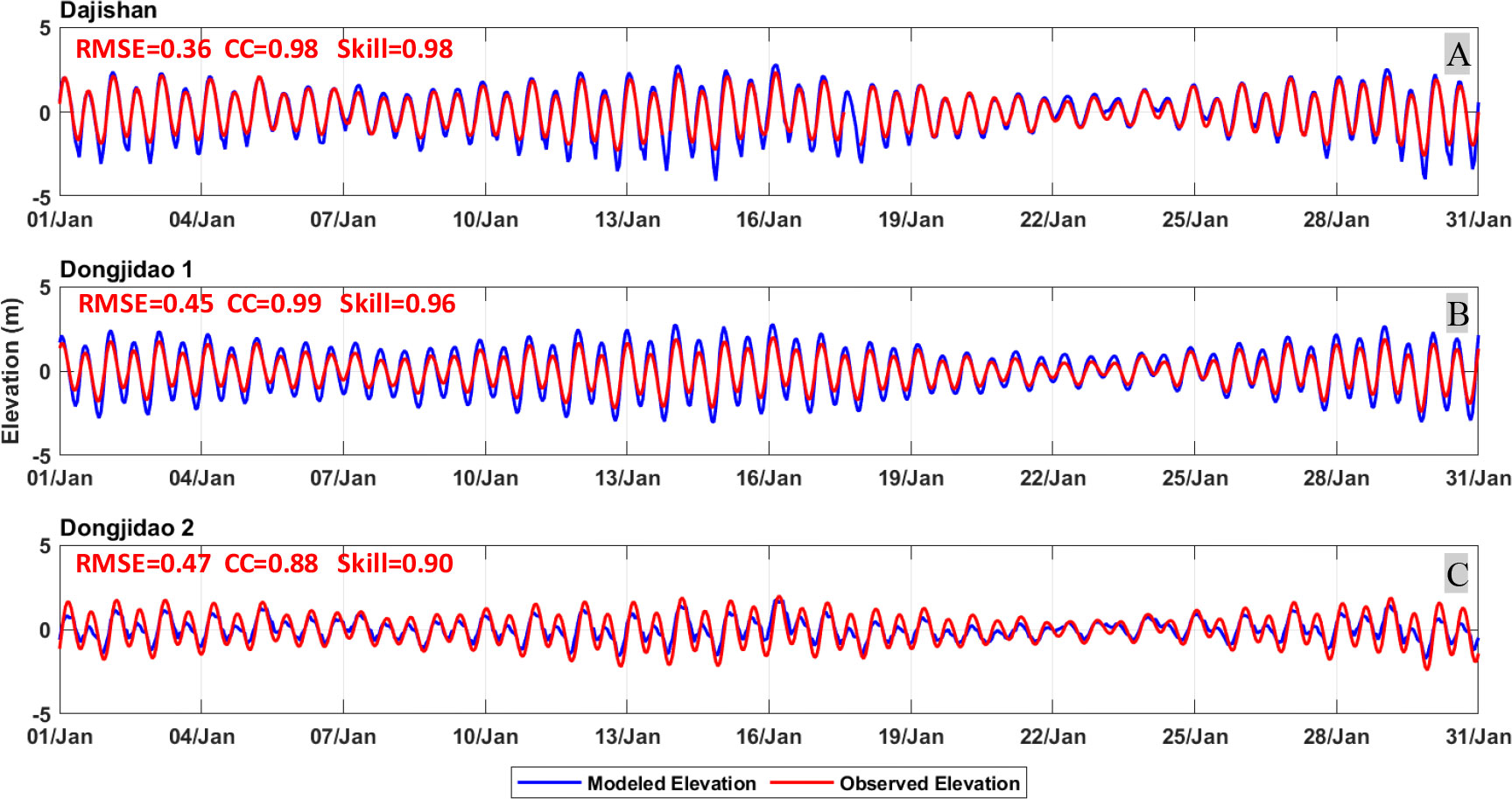
Figure 4 Comparison of modeled and observed elevations at three seafloor observation systems. Each station’s statistical parameters (RMSE, CC and Skill).
where η and ζ represent the modeled and the observed sea elevation, respectively, the overbar donates the temporal average. The RMSE of these stations are 0.36, 0.45, 0.47; CC are 0.98, 0.99, 0.88 and Skill are 0.98, 0.96, 0.90, respectively. The comparison indicates that the model has a good capability of simulating tidal motions in the study area.
Further, tidal harmonic analysis is applied using the T_TIDE MATLAB toolbox (Pawlowicz et al., 2002) to obtain the tidal harmonic constants of four major tidal components (M2, S2, K1 and O1) in those tide gauges around the Zhejiang-Fujian coast (black dots in Figure 1B). The comparisons of amplitude and phase of four major tidal constituents are shown in Tables 1 and 2. In general, model results have satisfying consistency with observations. The Mean Errors (ME) of the M2, S2, K1 and O1 tidal components are 0.30, 0.10, 0.04 and 0.03 m in amplitudes, 31.1°, 31.6°, 15.1° and 16.8° in phases, respectively. The simulation errors may come from the insufficient horizontal resolution near each tidal gauge. Nevertheless, such tidal performance of the coastal region model is acceptable in complicated coastline and bathymetry.
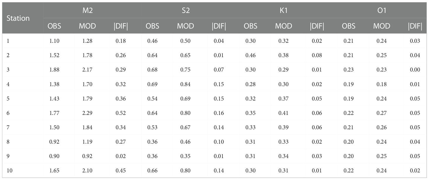
Table 1 The comparison of amplitudes (m) between the observation and simulation of the major four tidal components.
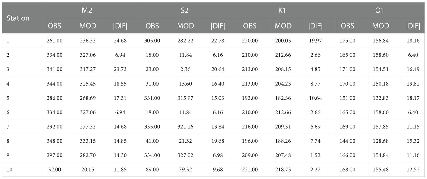
Table 2 The comparison of phases (°) between the observation and simulation of the major four tidal components.
The model performance in temperature is crucial for studying temperature fronts, therefore, we evaluated the model output of sea temperature from bottom to surface based on the seafloor observations, MODIS-Aqua SST and MURSST products. The comparison between the modeled and observed bottom temperature is shown in Figure 5. Due to lack of measurement, only observations at stations Dajishan and Yujing 5 were used to validate the modeled bottom temperature. Figure 5 shows that the model satisfyingly simulates both the magnitude and the trend of temperature variation from winter to autumn, only minor overestimation in summer and underestimation in winter occurred. Three statistical parameters RMSE, CC, and Skill are applied in this part as well. The relatively small RMSE, high CC and Skill at two stations suggest that the model could reasonably simulate the bottom temperature in the study area.
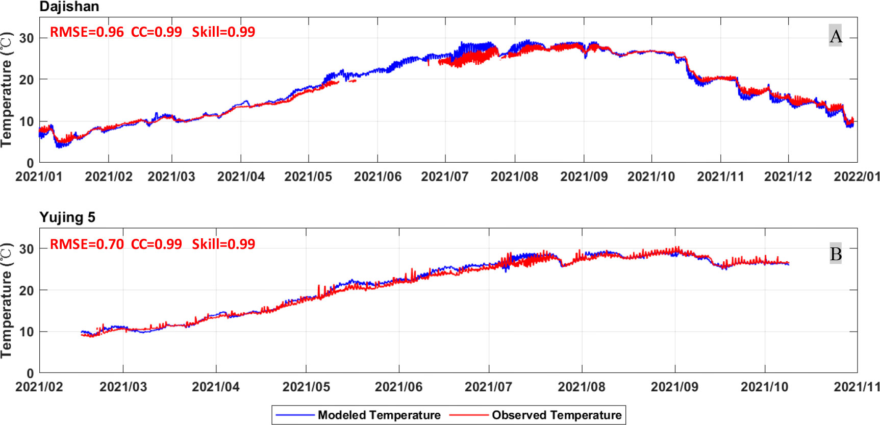
Figure 5 Comparison of modeled bottom temperature with the seafloor observation in Dajishan (A) and Yujing 5 (B).
The modeled SST is further validated by satellite SST products. Figure 6 compares the monthly-mean SST from October 2020 to March 2021, showing good consistency between the simulated and observed SST in spatial pattern (southward extension of the ZFCC and northwestward intrusion of KC) as well as in temperature values. Notably, the cold tongue which plays a significant role in the ZFCC off the Jiangsu coast is also well simulated.
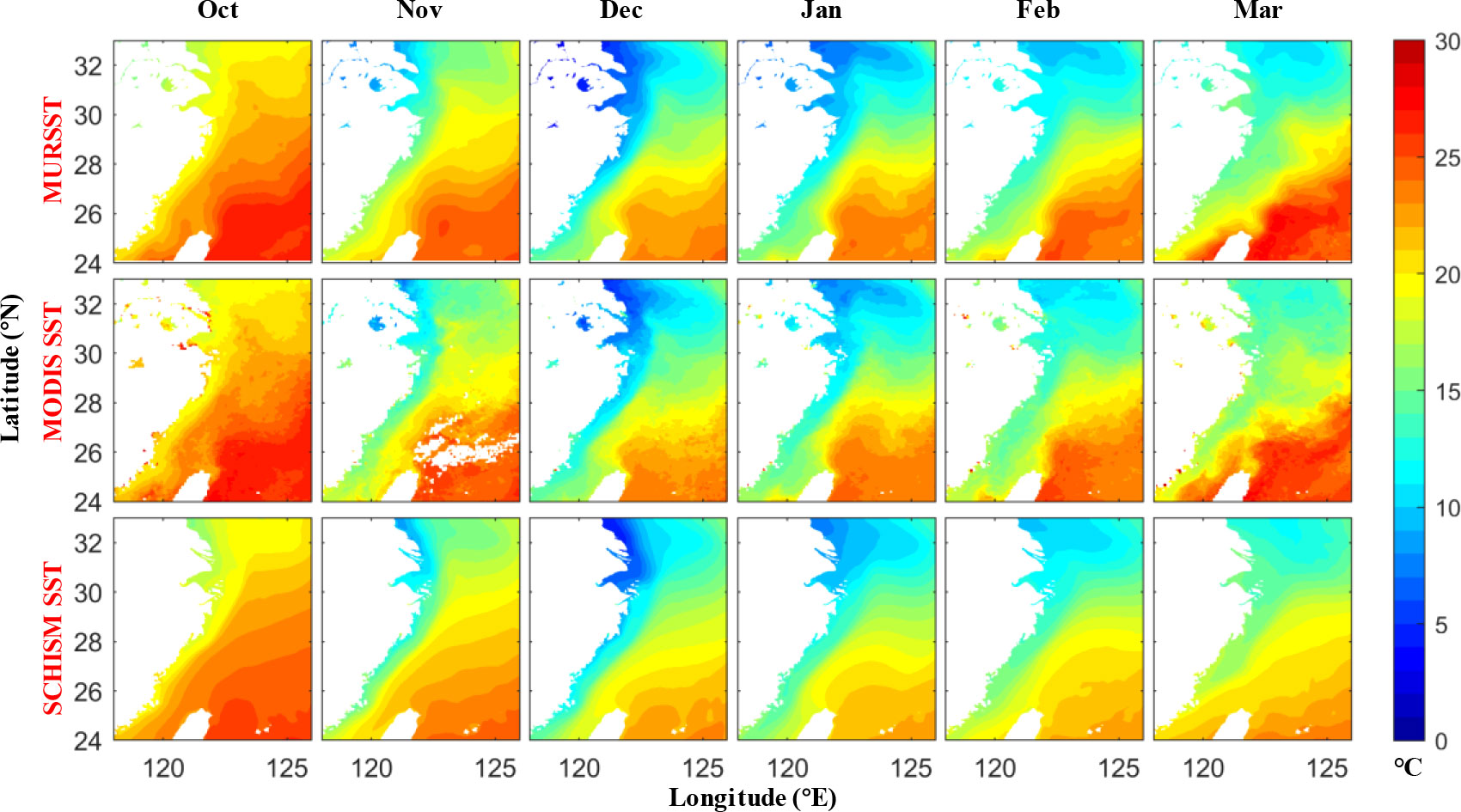
Figure 6 Comparison of monthly averaged SST between simulated and satellite-observed (MURSST and MODIS-Aqua) SST from October 2020 to March 2021.
In general, validations of simulated temperature at both surface and bottom layers indicate satisfactory model performance, which certainly ensures the reliability of following analyses.
As the large-scale background circulation remarkably dominates variation of ZFCF (Hsu et al., 2021), the modeled flow pattern is further evaluated. Figure 7 shows the surface current field off the Zhejiang-Fujian coast from October 2020 to March 2021, two main currents, the ZFCC and KC, can be easily distinguished from Figure 7. The ZFCC has a relatively high intensity in October, December and January due to the powerful northeast monsoon, it gradually weakens in February and March following the decay of prevailing monsoon. There are three major branches of KI north to Taiwan Island, the first- and second-branch turn southwestward and northward, and then merge with the downstream and midstream of ZFCC, respectively. The third branch turns westward but finally merges into the KC mainstream again. Compared with former investigations, the flow pattern produced by our model is in good consistence with previous investigations (Liu et al., 2014; Yang et al., 2018; Cui et al., 2021), again suggesting reliable model performance.
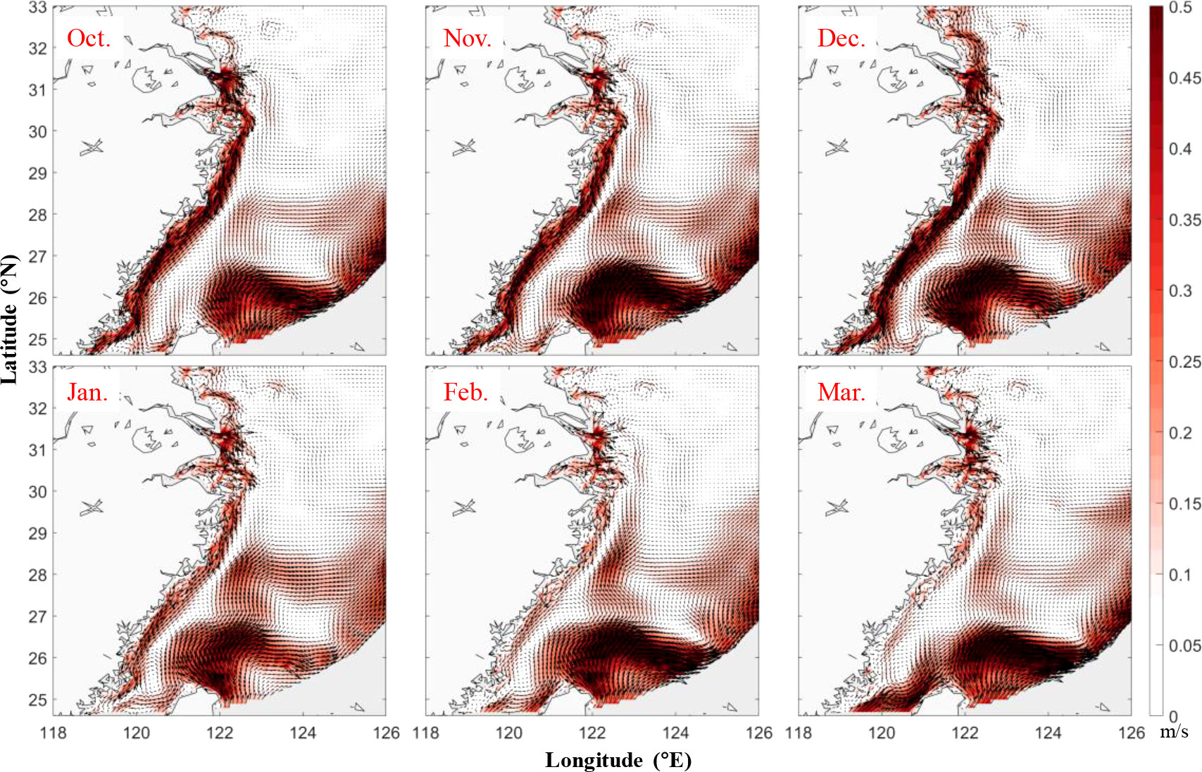
Figure 7 Monthly-average surface currents off the Zhejiang-Fujian coast from October 2020 to March 2021, the arrows represent the flow direction while color indicates current magnitude.
The vertical structure of temperature and current across the ZFCF in two representative sections (sec1 and sec3, Figure 1B.) from October 2020 to March 2021 are shown in Figures 8 and 9, respectively. As Figures 8A-F reveal, in October, despite the presence of strong ZFCC, no significant thermal fronts occurred because the water column is well stratified. As it comes to November, the whole water column is sufficiently mixed under the strong wind stress, meanwhile the cold ZFCC dominates the coastal area, therefore the horizontal temperature gradient begins to strengthen and an apparent thermal front (ZFCF) forms at regions 20~50 km off the coast. After reaching its peak in January, the vertical isotherm of the ZFCF gradually shifts direction and transforms into a horizontal distribution, suggesting the decay of ZFCF. From Figures 8G-L, the boundary of the northward and southward current can be clearly distinguished by the black dotted lines; interestingly, the boundary of two reversed current is located about 60 km off the coast, which is remarkably different with the location of ZFCF. This feature seems to be contradictory to the formation mechanism of the front raised by former studies, which will be explained in section 4. The first branch of KI carries relatively warm water and joins into the ZFCC near the coast. Thus, a front closer to the coast is formed. Meanwhile, the weakening of northward flow in January also suggests that the strong KI and northly monsoon could inhibit the southward flow within the Taiwan Strait. Obviously, Figure 8 provides a piece of clear evidence that the ZFCF is affected by the KI.
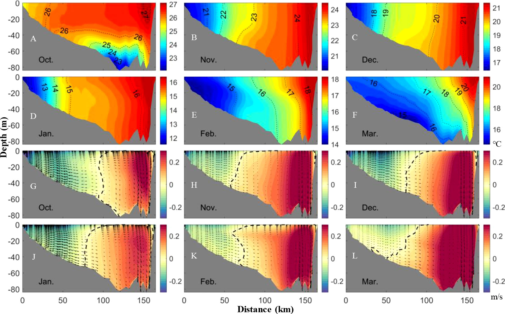
Figure 8 Vertical structure of temperature (A-F) and flow (G-L, along-isobath component in colors, northward positive; cross-isobath and vertical components in arrows, vertical velocity is multiplied by 1000) along sec1 from October 2020 to March 2021. The dotted lines in subgraphs (G–L) indicate the location of 0 m/s of along-isobath velocity.
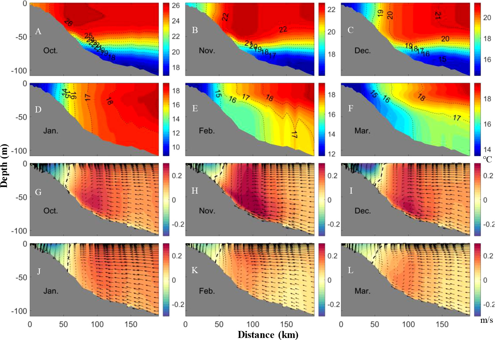
Figure 9 Same as Figure 8 but for sec 3.
Sec 3 is located at the junction of the Zhejiang and Fujian coasts. Along sec 3 (Figures 9A-F), the temperature structure of the upper water has the same pattern as sec 1 in regions shallower than 50 m, while the deep water has strong stratification during October to December. The water column could be well mixed only in January, and then it stratifies again accompanied by the weakening of the front. The variation in the stratification of the water column is usually dominated by the heat fluxes, and thus exerts potential impact on the ZFCF, which will be discussed in the next section. In addition, the flow structure reveals that the southward (ZFCC) and northward (TWC) flows have a clear decreasing tendency through February and March, which is a strong indicator that the change of background flow may be the direct cause of the abrupt change of ZFCF.
We have analyzed the three-dimension structure and variation of the ZFCF based on satellite observations and numerical results. Above analyses suggest that the abrupt change of ZFCF is closely related with the variations in wind, background circulation, and also the stratification. Moreover, we noticed that the decay of ZFCF still persisted even after the recovery of northerly wind. In this section, the roles of different dynamic factors will be carefully discussed based on correlation analysis, heat budget and a series of numerically diagnostic experiments.
The intensity of the ZFCF is closely related to the northeast monsoon (Figure 2): the monsoon weakened to some extent during the sudden drop of the ZFCF. Further, the stratification of the water column caused by variation of the net heat flux may also contribute to the sudden drop in thermal front (Figures 8 and 9). Therefore, based on correlation analysis, the relationships between the heat flux, wind stress, and the ZFCF were analyzed. We calculated the area-averaged local winds, net heat flux, and the SST gradient from January to March through 2003-2021 and the results are presented in Figure 10. As displayed, the intense heat loss (negative net heat flux) corresponds well with higher SST gradients, the regression analysis result (R=-0.72, P<0.001) also confirms their significant correlation. During a heat loss process, the shallow nearshore area tends to be cooled down more completely compared with the deep offshore region due to stronger vertical mixing and relatively lower heat content over the whole water column. Therefore, the temperature difference between nearshore and offshore waters gets further expanded, triggering a stronger ZFCF.
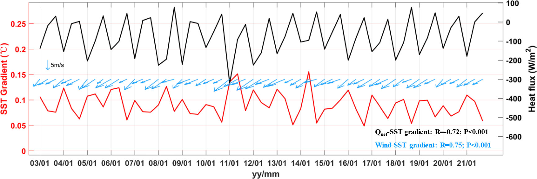
Figure 10 Comparison of the SST gradient magnitude (red line), surface net heat flux (black line, positive downwards) and wind stress vectors (blue arrows), all three are area-average results of the focus region. The correlation coefficients for the regression are labeled.
Winds can directly modulate the circulation, vertical mixing, and the air-sea heat exchange process (Qiao et al., 2006; Wang et al., 2015; Zhou et al., 2015; Park et al., 2020), further adjusting the ZFCF. Thus, as speculated, Figure 10 shows significant correlationship between SST gradient and wind stress (R=0.75, P<0.01). However, effect of winds on ZFCF is a comprehensive process and next we will explore the contribution of winds from different aspects.
The encounter of two different water masses or currents is one of the major frontogenesis mechanisms, as section 3.3 reveals, the weakening of ZFCC and TWC is highly correlated with the abrupt decay of ZFCF. We used the monthly-averaged HYCOM current product and MODIS-Aqua SST data to find out the relationship between the currents and ZFCF from January to March over an interannual scale. Expect for sec 1 and 3 presented above, two more sections (sec 2 and 4, Figure 1B) are selected to investigate the role of KI. The heat flux QT through four representative sections are calculated to diagnose the interactions between the background flow and ZFCF following:
where T is the temperature of the water column, V is the cross-section velocity, η is sea water level, h is the water depth, and l is the width of the section. The southward current through sec 1 and 3 represent the ZFCC, while the northward current across sec 1 represents the flow through Taiwan Strait, and the westward currents crossing sec 2 and 4 represent the KI.
Figure 11 shows the time series of area-averaged SST gradient and QT through sec 1-4, meanwhile, results of linear regression analysis (at 95% confidence level) are shown in Table 3. For the ZFCC (southward current through sec 1 and 3), the variation of QT and SST gradient synchronize well with each other and significantly correlated (R=0.46 and 0.56, respectively). The ZFCC flows southward along the coast, bringing cold and fresh water to the focus area, and therefore directly maintains and regulates the ZFCF.
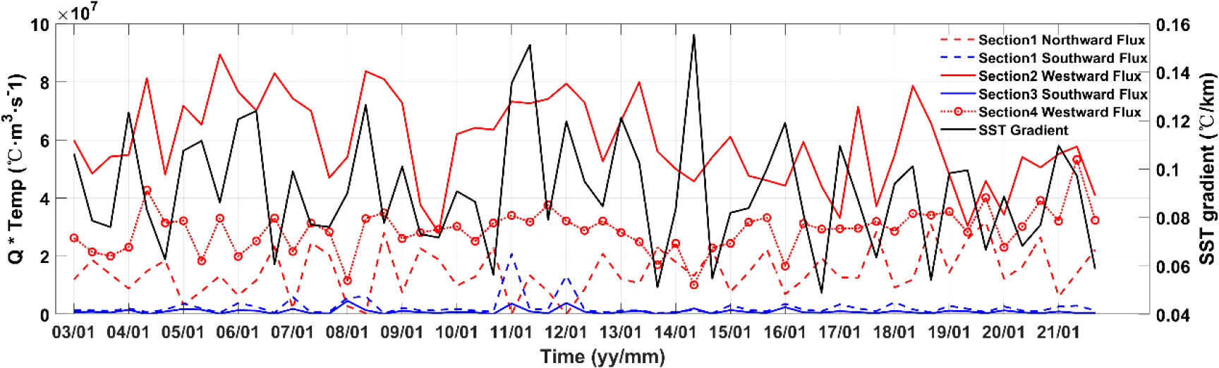
Figure 11 Time series of QT (heat flux) through four representative sections and the area-averaged SST gradient.
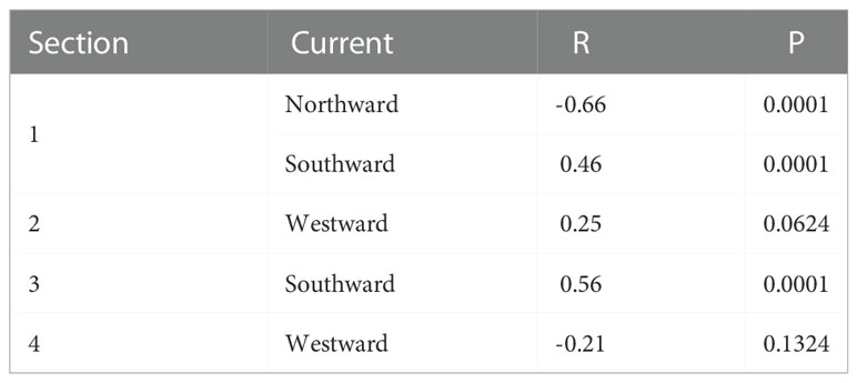
Table 3 Results of linear regression analysis between QT and SST gradient.
For the warm flow through Taiwan strait (northward current across sec 1), it leads to a significantly negative correlation between the QT and SST gradient (R=-0.66, P<0.001). This seems to be inconsistent with common sense, as the encounter of two different flows with larger temperature gradients tends to establish a strong thermal front. And here, the Taiwan Strait current and ZFCC have opposite directions, strong northerly winds will strengthen southward ZFCC and weaken northward Taiwan Strait current, thus the QT of Taiwan Strait current through sec 1 is reducing. The ZFCC and TWC could be regarded as the cool and warm water sources for forming ZFCF, when TWC weakens, extra warm water sources are needed to maintain the strength of ZFCF. For the ZFCF, KI is the possible one which might supply warm water except for the Taiwan Strait current.
Wang and Oey (2014) indicated that the strengthened northeast wind would significantly enhance the KI. Recently, Kang and Na (2022) further reported significant correlation relationships between KI and wind stress and wind stress curl. Does this mean stronger northeast winds will generate stronger KI, and thus leads to a stronger ZFCF? The answer is uncertain because stronger northeast winds enhance the KI but will inhibit the northward transport of warm KC water. This is why Figure 11 and Table 3 both suggest no significant relationship between the KI (westward current in sec 2 and 4) and the SST gradient.
Discussions above point out that the ZFCF is closely modulated by the heat flux and background circulation in long term. To find out the key factors leading to this abrupt change of ZFCF in early spring, 2021, heat budget analysis was conducted based on numerical results. Since the onshore water column was well mixed during the abrupt change, we selected a series of representative points (blue and red dots in Figure 12E) located on either side of ZFCF, and the average heat budget through the whole water column at each point was calculated following Vijith et al. (2020) and the equation was written as:
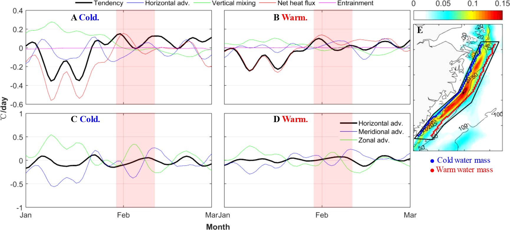
Figure 12 (A, B) Time series of the terms of the heat budget equation in cold water (blue dots in E) and warm water (red dots in E), the red shaded represents the same abrupt change period as Figure 3. (C, D) Zonal and meridional components of the horizontal advection in cold and warm water. (E) Average modeled SST gradient of January to March, 2021, and the points used for heat budget analysis.
Where T, ρ0, cp and h represent the temperature, mean density, water column depth and specific heat capacity of seawater, respectively. u,v and w are the zonal, meridional and vertical velocity. The suffix a are the vertically-averaged quantity and the subscript -h denotes the quantity at the base of the water column. q0 and qpen are the surface net heat flux and penetrative loss of shortwave radiation, respectively. KH and Kz represent the horizontal and vertical eddy diffusivities, respectively.
The sum of the horizontal advection, horizontal mixing, vertical mixing, entrainment and net heat flux well consist the overall pattern of the tendency term with a correlation of 0.87 and 0.83, RMSE of 0.13 and 0.09 °C/day (within 95% confidence interval) in cold water and warm water, respectively. The result is a satisfyingly good closure of the whole water column heat budget for such short time scales. Our analysis points out that net heat flux is important in determining the net tendency of the temperature on both sides of the front (Figures 12A and B), while in the cold water west to the front, vertical mixing and horizontal advection also greatly contribute to the tendency before February. For the abrupt change around later January, the temperature tendency in cold water has already been positive, while that in warm water east to the front was still negative. That indicates the temperature in cold water begins to warm up thus the temperature difference between two water masses is reduced. When the positive tendency reached its peak (~0.18°C/day) in cold water, the intensity of the ZFCF starts abruptly decreasing, and the net heat flux was the predominant contributor.
Interestingly, during the change period, the contributor of the positive tendency changed from net heat flux to horizontal advection in cold water, which provides a good answer to the question at the end of section 3.1. Although the recovery of the monsoon causes the net heat flux tends to cool the onshore water again, the heat carried by the horizontal advection compensated for the loss and kept the tendency positive, then resulting the decrease of ZFCF in the second period. Besides, the decomposition of the horizontal advection reveals that the flow pattern might change during the abrupt change of the ZFCF, because the zonal advection term changed from positive to negative and the meridional advection changed from negative to positive on both sides of the front. Combined with the analysis of the above sections, the variations of the horizontal advection of ZFCC and KI might induce the positive temperature tendency.
To further illustrate the contributions of different dynamic factors in triggering the abrupt decay of ZFCF in February, we conducted a series of sensitive numerical experiments based on above analyses. Each experiment runs for seven months from October 1, 2020, the control conditions of these sensitive experiments are listed in Table 4.
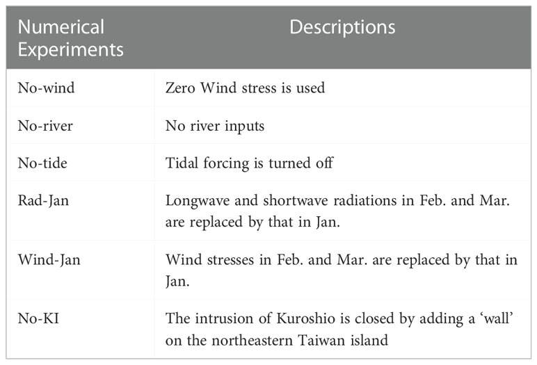
Table 4 Key configurations of sensitive experiments.
The differences in SST gradient between the sensitive experiments and control run are shown in Figure 13. When the wind stress forcing is closed (No-wind case), the SST gradient have changed dramatically in both distribution and intensity, the ZFCF almost disappears; in this case, thermal fronts mainly occurred around the Yangtze River estuary or regions with complicated bathymetry as a result of river discharge and modulation of current by topography. Moreover, the fronts triggered by the KI to the northeast of Taiwan Island are further away from the shelf, indicating a decreased KI under weak northerly monsoon, which agrees well with previous study (Wang and Oey, 2014). We found that the ZFCC almost disappeared with a small velocity lower than 0.1 m/s; thus, local wind stress is a key factor during the formation of ZFCF through modulating the intensity of ZFCC. When the wind stress in February and March were replaced by that in January (Exp. Wind-Jan, Figure 13E), the ZFCF was significantly enhanced, again proving that the weakening of the northeast wind stress plays a vital role during the abrupt decay process in February and March.
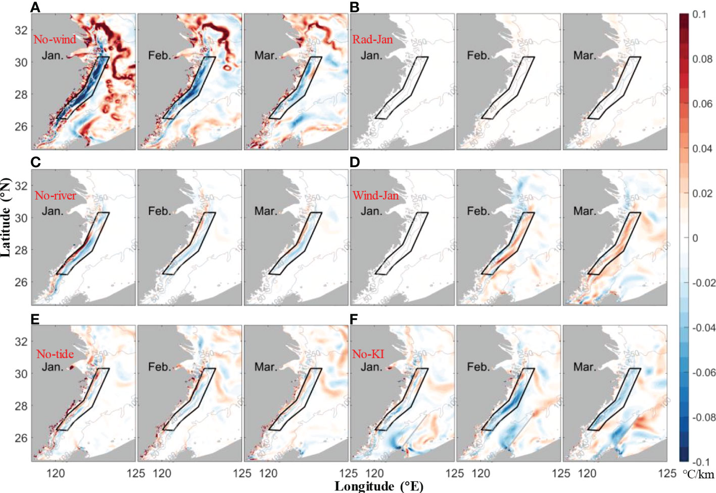
Figure 13 Differences in SST gradient between six sensitive experiments and the control run (A–F). The focus region is marked off with a black polygon.
When no river discharge was considered (Exp. No-river, Figure 13B), the location of ZFCF is closer to the coastline in January compared with the control run, besides, the intensity of ZFCF decreases slightly in February and March. As an essential component of the ZFCC, the riverine flow merges with the ZFCC, increasing the flow flux and strengthening the zonal width of the ZFCC (Wu et al., 2021), which then leads to a farther ZFCF off the coast. Besides, buoyancy forcing produced by the Yangtze River discharge can strengthen the southward flow of the Zhejiang-Fujian coastal water (Wu et al., 2021; Zhang et al., 2022), so the ZFCF decreases in February and March under the condition of no river discharge. Further, runoff of the Yangtze River reduced from January (40.6×10⁹ m3) to February (33.53×10⁹ m3), which might also contribute to the decrease of the ZFCF in February.
From experiments No-tide and Rad-Jan (Figures 13C and D), limited effect of solar radiation and tidal forcing on the intensity of ZFCF could be speculated, and the front is fixed on the topographic slope under the tidal mixing (Cheng et al., 2017). When tidal forcing is neglected, the location of the front moves onshore. Moreover, the result also points out that the net heat flux, which is important in determining the net temperature tendency, is mainly modulated by latent and sensible heat flux controlled by winds.
To investigate the influence of the KI, Exp. No-KI was designed by blocking the western passage of the KI (Figure 13F) to simulate the situation of the weak KI. Notably, KI and the shelf circulation are vital components of the ECS, to balance the mass flux in and out of the continental shelf, when the KI was cut off, the currents through the Taiwan Strait will be influenced (Yang et al., 2020; Wu, 2021). In this case, the front formed by the KI in northern Taiwan Island has disappeared completely, meanwhile, the ZFCF has significantly changed. The reduction of frontal intensity in January is much weaker than that in February and March, this phenomenon indicates that the KI can hardly reach the focus region under the strong northeast monsoon in January, so the reduction of ZFCF in the southern area is much remarkable than that in the northern area. Tracer experiments by Yang et al. (2018) suggested that the Kuroshio subsurface water cannot reach the algal bloom area along the Zhejiang coast in winter, when the prevailing monsoon relaxes, the onshore intrusion of the Kuroshio will be less prohibited by the barotropic pressure force created by the onshore Ekman transport (Yang et al., 2012; Xu et al., 2018). The intensity of ZFCF decreases distinctly in February under the absence of the KI, the maximum reduction reaches 0.08 °C/km inside the focus region, which is comparable with the change in the No-wind experiment, and even larger in March. Exp. No-KI indicates that the ZFCF is formed by the southward advection of the ZFCC, which was mainly forced by the northeast wind forcing, and the TWC water. As Figure 13F revealed, only a minor change of ZFCF occurred in January when the KI is cut off. However, this circumstance changed dramatically in Feb and Mar when the prevailing monsoon relaxed. This is attributed to the impact of KI, which can reach the focus region and then further affect the ZFCF more efficiently under the weak northeast monsoon. At this point, assisted by the heat budget analysis, the mechanism of the decrease in the second period can be revealed. During the weak of ZFCF in the first period which was caused by relaxation of the monsoon, the invaded water tended to transport to the focus region at the same time. And after this period of monsoon relaxation, the invaded water reached the focus area and heated the weak ZFCC water, so the component of horizontal advection term contributed positive temperature tendency changed from zonal shelf warm water advection to meridional KI advection (Figures 12C and D). Although, the monsoon recovered and tended to cool the onshore water again, the heating effect by KI was stronger than wind cooling effect, thus ZFCF was continually weakening in the second period until the winds forced the cool ZFCC southward and impeded the northward transport of the KI water again. However, Figure 3 shows that the intensity of ZFCF gets stronger after the abrupt decrease, which is caused by the interaction of cool water forced by recovered winds and the residual warm KI water left on the shelf. Also, in the following period with relatively weak northeast monsoon, the continuously invaded water maintained the less intense ZFCF until the onshore water was heating up in the middle March.
Former investigations have clarified the spatiotemporal variation of the ZFCF on seasonal scale as well as the basic mechanism of its variation, however, the abrupt change of the ZFCF on short-time scale requires to be further explored. Based on the multi-source satellite data, we found that the ZFCF has an abrupt change in early Spring, to improve understanding of the sudden variation and its internal mechanism of the ZFCF, we used a three-dimensional numerical model to simulate the variability of the coastal front along the ECS, investigated the key controlling factors of the variability of the ZFCF and revealed the main reason for its abrupt change in February.
Based on long-term regression analysis, heat budget analysis and sensitivity experiment, we found that the variation of wind stress is the main factor in the formation and disappearance of the ZFCF. The ZFCC and the KI, influenced by wind, heat flux and river discharge, are two key factors controlling the intensity and region of the ZFCF. For the abrupt change of the ZFCF in early spring, 2021, heat budget analysis indicated that net heat flux and horizontal advection were the most significant terms in determining the net temperature tendency difference between the two water masses of the ZFCF. Followed sensitivity experiment pointed out that the variation of the net heat flux is mainly modulated by the winds and the temperature tendency contributed by horizontal advection is affected by KI and ZFCC. In later January, under the relaxation of the northeast monsoon, the intensity of the ZFCC weakened subsequently, directly inducing the abruptly decreasing of the ZFCF in the first period. Then a second period decrease followed after the KI water transported to the focus region even if the northeast monsoon was recovered. The heating effect of the invaded water was stronger than the cooling effect of the wind, thus the intensity of the ZFCF kept decreasing until the monsoon forced the ZFCC southwardly and impeded the northward transport of the KI again.
The ZFCC and KI, closely associated with the abrupt change of the thermal front, delivered the eutrophication, phosphate and heat to the Zhejiang-Fujian coastal area, respectively, which will impact the algal bloom or other ecosystem influence (Lian et al., 2016; Zhang et al., 2018; Liu et al., 2021). However, the biogeochemical responses associated with the coastal front plunge remain to be investigated by the field or remote sensing observation to fully understand the regional dynamics in the future. In addition, this finding also provides a shred of specific evidence for the source of Taiwan Warm water in winter.
The original contributions presented in the study are included in the article/supplementary material. Further inquiries can be directed to the corresponding authors.
JL and WW analyzed and visualized the data and wrote the manuscript. PL conceived the study and provided the methods and resources. FZ and YG reviewed and edited the manuscript. PB assisted with the formal analysis, and reviewed and edited the manuscript. All authors contributed to the article and approved the submitted version.
This study was jointly financed by the National Natural Science Foundation of China (Grant Number 42106017), the Scientific and technological projects of Zhoushan (Grant Number 2022C81010), the Guangdong Basic and Applied Basic Research Foundation (Grant Number 2020A1515110516), the Special Fund for Technology Development of Zhanjiang City (Grant Number 2020A01008), and the Scientific Research Foundation for Advanced Talents of Zhejiang Ocean University (Grant Number 11105093522), the Key Research and Development Plan of Zhejiang Province Funding (Grant Number 2020C03012), the Major Science and Technology Project of Sanya (Grant Number SKJC-KJ-2019KY03), the High-level Personnel of Special Support Program of Zhejiang Province (Grant Number 2019R52045), the Science Foundation of Donghai Laboratory (Grant Number DH-2022KF0208) and the Hainan Provincial Joint Project of Sanya Yazhou Bay Science and Technology City (Grant Number 120LH001).
The authors declare that the research was conducted in the absence of any commercial or financial relationships that could be construed as a potential conflict of interest.
All claims expressed in this article are solely those of the authors and do not necessarily represent those of their affiliated organizations, or those of the publisher, the editors and the reviewers. Any product that may be evaluated in this article, or claim that may be made by its manufacturer, is not guaranteed or endorsed by the publisher.
Alemany D., Acha E. M., Iribarne O. O. (2014). Marine fronts are important fishing areas for demersal species at the Argentine Sea (Southwest Atlantic ocean). J. Sea Res. 87, 56–67. doi: 10.1016/j.seares.2013.12.006
Androulidakis Y., Kourafalou V., Ozgokmen T., Garcia-Pineda O., Lund B., Le Henaff M., et al. (2018). Influence of river-induced fronts on hydrocarbon transport: A multiplatform observational study. J. Geophys. Res.-Oceans 123 (5), 3259–3285. doi: 10.1029/2017JC013514
Bai P., Gu Y., Li P., Wu K. (2016). Tidal energy budget in the zhujiang (Pearl river) estuary. Acta Oceanol. Sin. 35 (5), 54–65. doi: 10.1007/s13131-016-0850-9
Belkin I. M., O'Reilly J. E. (2009). An algorithm for oceanic front detection in chlorophyll and SST satellite imagery. J. Mar. Syst. 78 (3), 319–326. doi: 10.1016/j.jmarsys.2008.11.018
Bian C., Jiang W., Quan Q., Wang T., Greatbatch R. J., Li W. (2013). Distributions of suspended sediment concentration in the yellow Sea and the East China Sea based on field surveys during the four seasons of 2011. J. Mar. Syst. 121, 24–35. doi: 10.1016/j.jmarsys.2013.03.013
Cao L., Tang R., Huang W., Wang Y. (2021). Seasonal variability and dynamics of coastal sea surface temperature fronts in the East China Sea. Ocean Dyna. 71 (2), 237–249. doi: 10.1007/s10236-020-01427-8
Chen C.-T. A. (2009). Chemical and physical fronts in the bohai, yellow and East China seas. J. Mar. Syst. 78 (3), 394–410. doi: 10.1016/j.jmarsys.2008.11.016
Cheng X., Sun Q., Wang Y., Yang Y. (2017). Analysis on seasonal variations and structures of the tidal front outside of the subei shoal. Mar. Sci. 41 (12), 1. doi: 10.11759/hykx20151108001
Cromwell T., Reid J. L. (1956). A study of oceanic fronts. Tellus 8 (1), 94–101. doi: 10.3402/tellusa.v8i1.8947
Cui X., Yang D., Sun C., Feng X., Gao G., Xu L., et al. (2021). New insight into the onshore intrusion of the kuroshio into the East China Sea. J. Geophys. Res.: Oceans 126 (2), e2020JC016248. doi: 10.1029/2020JC016248
He S., Huang D., Zeng D. (2016). Double SST fronts observed from MODIS data in the East China Sea off the zhejiang–fujian coast, China. J. Mar. Syst. 154, 93–102. doi: 10.1016/j.jmarsys.2015.02.009
Hickox R., Belkin I., Cornillon P., Shan Z. (2000). Climatology and seasonal variability of ocean fronts in the East China, yellow and bohai seas from satellite SST data. Geophys. Res. Lett. 27 (18), 2945–2948. doi: 10.1029/1999GL011223
Hsieh C.-h., Chiu T.-S., Shih C.-T. (2004). Copepod diversity and composition as indicators of intrusion of the kuroshio branch current into the northern Taiwan strait in spring 2000. Zool. Stud. 43 (2), 393–403. doi: 10.3390/biology11091357
Hsu P.-C., Centurioni L., Shao H.-J., Zheng Q., Lu C.-Y., Hsu T.-W., et al. (2021). Surface current variations and oceanic fronts in the southern East China Sea: Drifter experiments, coastal radar applications, and satellite observations. J. Geophys. Res.: Oceans 126 (10), e2021JC017373. doi: 10.1029/2021JC017373
Huang D., Zhang T., Zhou F. (2010). Sea-Surface temperature fronts in the yellow and East China seas from TRMM microwave imager data. Deep Sea Res. Part II: Top. Stud. Oceanogr. 57 (11-12), 1017–1024. doi: 10.1016/j.dsr2.2010.02.003
Hu Z. F., Wang D. P., Pan D. L., He X. Q., Miyazawa Y., Bai Y., et al. (2016). Mapping surface tidal currents and changjiang plume in the East China Sea from geostationary ocean color imager. J. Geophys. Res.-Oceans 121 (3), 1563–1572. doi: 10.1002/2015JC011469
Isobe A. (2008). Recent advances in ocean-circulation research on the yellow Sea and East China Sea shelves. J. oceanogr. 64 (4), 569–584. doi: 10.1007/s10872-008-0048-7
Kang J., Na H. (2022). Long-term variability of the kuroshio shelf intrusion and its relationship to upper-ocean current and temperature variability in the East China Sea. Front. Mar. Sci. 9. doi: 10.3389/fmars.2022.812911
Komatsu T., Tatsukawa K., Filippi J. B., Sagawa T., Matsunaga D., Mikami A., et al. (2007). Distribution of drifting seaweeds in eastern East China Sea. J. Mar. Syst. 67 (3-4), 245–252. doi: 10.1007/978-1-4020-9619-8_44
Lai W., Pan J., Devlin A. T. (2018). Impact of tides and winds on estuarine circulation in the pearl river estuary. Continent. Shelf Res. 168, 68–82. doi: 10.1016/j.csr.2018.09.004
Lian E., Yang S., Wu H., Yang C., Li C., Liu J. T. (2016). Kuroshio subsurface water feeds the wintertime Taiwan warm current on the inner East China Sea shelf. J. Geophys. Res.: Oceans 121 (7), 4790–4803. doi: 10.1002/2016JC011869
Liu X., Dong C., Chen D., Su J. (2014). The pattern and variability of winter kuroshio intrusion northeast of Taiwan. J. Geophys. Res.: Oceans 119 (8), 5380–5394. doi: 10.1002/2014JC009879
Liu Z., Gan J., Hu J., Wu H., Cai Z., Deng Y. (2021). Progress of studies on circulation dynamics in the East China Sea: The kuroshio exchanges with the shelf currents. Front. Mar. Sci. 8. doi: 10.3389/fmars.2021.620910
Liu S. D., Qiao L. L., Li G. X., Shi J. H., Huang L. L., Yao Z. G., et al. (2018). Variation in the current shear front and its potential effect on sediment transport over the inner shelf of the East China Sea in winter. J. Geophys. Res.-Oceans 123 (11), 8264–8283. doi: 10.1029/2018JC014241
Lohmann R., Belkin I. M. (2014). Organic pollutants and ocean fronts across the Atlantic ocean: A review. Prog. Oceanogr. 128, 172–184. doi: 10.1016/j.pocean.2014.08.013
Mao H. (1964). A preliminary investigation on the application of using TS diagram for a quantitative analysis of the water masses in the shallow water area. Oceanol. Limnol. Sin. 6, 1–22.
McWilliams J. C. (2021). Oceanic frontogenesis. Annu. Rev. Mar. Sci. 13, 227–253. doi: 10.1146/annurev-marine-032320-120725
Park G. S., Lee T., Min S.-H., Jung S.-K., Son Y. B. (2020). Abnormal Sea surface warming and cooling in the East China Sea during summer. J. Coast. Res. 95 (SI), 1505–1509. doi: 10.2112/SI95-290.1
Pawlowicz R., Beardsley B., Lentz S. (2002). Classical tidal harmonic analysis including error estimates in MATLAB using T_TIDE. Comput. Geosci. 28 (8), 929–937. doi: 10.1016/S0098-3004(02)00013-4
Qiao L., Liu S., Xue W., Liu P., Hu R., Sun H., et al. (2020). Spatiotemporal variations in suspended sediments over the inner shelf of the East China Sea with the effect of oceanic fronts. Estuar. Coast. Shelf Sci. 234, 106600. doi: 10.1016/j.ecss.2020.106600
Qiao F., Yang Y., Lü X., Xia C., Chen X., Wang B., et al. (2006). Coastal upwelling in the East China Sea in winter. J. Geophys. Res.: Oceans 111 (C11S06). doi: 10.1029/2005JC003264
Saldias G. S., Hernandez W., Lara C., Munoz R., Rojas C., Vasquez S., et al. (2021). Seasonal variability of SST fronts in the inner Sea of chiloe and its adjacent coastal ocean, northern Patagonia. Remote Sens. 13 (2), 181. doi: 10.3390/rs13020181
Saldias G. S., Lara C. (2020). Satellite-derived sea surface temperature fronts in a river-influenced coastal upwelling area off central-southern Chile. Reg. Stud. Mar. Sci. 37, 101322. doi: 10.1016/j.rsma.2020.101322
Teng F., Fang G. H., Xu X. Q. (2017). Effects of internal tidal dissipation and self-attraction and loading on semidiurnal tides in the bohai Sea, yellow Sea and East China Sea: a numerical study. Chin. J. Oceanol. Limnol. 35 (5), 987–1001. doi: 10.1007/s00343-017-6087-4
Tozer B., Sandwell D. T., Smith W. H. F., Olson C., Beale J. R., Wessel P. (2019). Global bathymetry and topography at 15 arc sec: SRTM15+. Earth Space Sci. 6 (10), 1847–1864. doi: 10.1029/2019EA000658
Tseng C., Lin C., Chen S., Shyu C. (2000). Temporal and spatial variations of sea surface temperature in the East China Sea. Continent. Shelf Res. 20 (4-5), 373–387. doi: 10.1016/S0278-4343(99)00077-1
Vazquez-Cuervo J., Dewitte B., Chin T. M., Armstrong E. M., Purca S., Alburqueque E. (2013). An analysis of SST gradients off the Peruvian coast: The impact of going to higher resolution. Remote Sens. Environ. 131, 76–84. doi: 10.1016/j.rse.2012.12.010
Vijith V., Vinayachandran P. N., Webber B. G. M., Matthews A. J., George J. V., Kannaujia V. K., et al. (2020). Closing the sea surface mixed layer temperature budget from in situ observations alone: Operation advection during BoBBLE. Sci. Rep. 10 (1), 7062. doi: 10.1038/s41598-020-63320-0
Wang G., Kang J., Yan G., Han G., Han Q. (2015). Spatio-temporal variability of sea level in the East China Sea. J. Coast. Res. 73 (10073), 40–47. doi: 10.2112/SI73-008.1
Wang J., Oey L. Y. (2014). Inter-annual and decadal fluctuations of the kuroshio in East China Sea and connection with surface fluxes of momentum and heat. Geophys. Res. Lett. 41 (23), 8538–8546. doi: 10.1002/2014GL062118
Wang Y., Sheng J. Y., Lu Y. Y. (2020). Examining tidal impacts on seasonal circulation and hydrography variability over the eastern Canadian shelf using a coupled circulation-ice regional model. Prog. Oceanogr. 189. doi: 10.1016/j.pocean.2020.102448
Wu H. (2021). Beta-plane arrested topographic wave as a linkage of open ocean forcing and mean shelf circulation. J. Phys. Oceanogr. 51 (3), 879–893. doi: 10.1175/jpo-d-20-0195.1
Wu H., Deng B., Yuan R., Hu J., Gu J. H., Shen F., et al. (2013). Detiding measurement on transport of the changjiang-derived buoyant coastal current. J. Phys. Oceanogr. 43 (11), 2388–2399. doi: 10.1175/JPO-D-12-0158.1
Wu R., Wu H., Wang Y. (2021). Modulation of shelf circulations under multiple river discharges in the East China Sea. J. Geophys. Res.: Oceans 126 (4), e2020JC016990. doi: 10.1029/2020JC016990
Xu L., Yang D., Benthuysen J. A., Yin B. (2018). Key dynamical factors driving the kuroshio subsurface water to reach the zhejiang coastal area. J. Geophys. Res.: Oceans 123 (12), 9061–9081. doi: 10.1029/2018JC014219
Yang D., Huang R. X., Feng X., Qi J., Gao G., Yin B. (2020). Wind stress over the pacific ocean east of Japan drives the shelf circulation east of China. Continent. Shelf Res. 201, 104122. doi: 10.1016/j.csr.2020.104122
Yang D., Yin B., Chai F., Feng X., Xue H., Gao G., et al. (2018). The onshore intrusion of kuroshio subsurface water from February to July and a mechanism for the intrusion variation. Prog. Oceanogr. 167, 97–115. doi: 10.1016/j.pocean.2018.08.004
Yang D., Yin B., Liu Z., Bai T., Qi J., Chen H. (2012). Numerical study on the pattern and origins of kuroshio branches in the bottom water of southern East China Sea in summer. J. Geophys. Res.: Oceans 117, C02014. doi: 10.1029/2011JC007528
Zhai F., Li P., Gu Y., Li X., Chen D., Li L., et al. (2020). Review of the research and application of the submarine cable online observation system. Mar. Sci. 44 (8), 14–28. doi: 10.11759/hykx20200331003
Zhang Y., Chai F., Zhang J., Ding Y., Bao M., Yan Y. W., et al. (2022). Numerical investigation of the control factors driving zhe-Min coastal current. Acta Oceanol. Sin. 41 (2), 127–138. doi: 10.1007/s13131-021-1849-4
Zhang C., Shang S., Chen D., Shang S. (2005). Short-term variability of the distribution of zhe-Min coastal water and wind forcing during winter monsoon in the Taiwan strait. J. OF Remote SENSING-BEIJING- 9 (4), 452. doi: 10.11849/zrzyxb.1991.01.010
Zhang Y. L. J., Stanev E. V., Grashorn S. (2016a). Unstructured-grid model for the north Sea and Baltic Sea: Validation against observations. Ocean Model. 97, 91–108. doi: 10.1016/j.ocemod.2015.11.009
Zhang Z., Wu H., Yin X., Qiao F. (2018). Dynamical response of changjiang river plume to a severe typhoon with the surface wave-induced mixing. J. Geophys. Res.: Oceans 123 (12), 9369–9388. doi: 10.1029/2018JC014266
Zhang Y. L. J., Ye F., Stanev E. V., Grashorn S. (2016b). Seamless cross-scale modeling with SCHISM. Ocean Model. 102, 64–81. doi: 10.1016/j.ocemod.2016.05.002
Keywords: thermal front, schism, Kuroshio intrusion, East China Sea, net heat flux
Citation: Li J, Li P, Bai P, Zhai F, Gu Y, Liu C, Sun R and Wu W (2022) Abrupt change of a thermal front in a high-biomass coastal zone during early spring. Front. Mar. Sci. 9:1092984. doi: 10.3389/fmars.2022.1092984
Received: 08 November 2022; Accepted: 05 December 2022;
Published: 15 December 2022.
Edited by:
Hui Zhao, Guangdong Ocean University, ChinaReviewed by:
Wenjin Sun, Nanjing University of Information Science and Technology, ChinaCopyright © 2022 Li, Li, Bai, Zhai, Gu, Liu, Sun and Wu. This is an open-access article distributed under the terms of the Creative Commons Attribution License (CC BY). The use, distribution or reproduction in other forums is permitted, provided the original author(s) and the copyright owner(s) are credited and that the original publication in this journal is cited, in accordance with accepted academic practice. No use, distribution or reproduction is permitted which does not comply with these terms.
*Correspondence: Peng Bai, cGVuZ2JhaUB6am91LmVkdS5jbg==; Yanzhen Gu, Z3V5YW56aGVuQHpqdS5lZHUuY25u
Disclaimer: All claims expressed in this article are solely those of the authors and do not necessarily represent those of their affiliated organizations, or those of the publisher, the editors and the reviewers. Any product that may be evaluated in this article or claim that may be made by its manufacturer is not guaranteed or endorsed by the publisher.
Research integrity at Frontiers
Learn more about the work of our research integrity team to safeguard the quality of each article we publish.