Characteristics of Eulerian mesoscale eddies in the Gulf of Mexico

Although numerous studies on Eulerian mesoscale eddies with closed contours of sea surface height (SSH) or streamline have been conducted in the Gulf of Mexico (GoM), a comprehensive study on their temporal and spatial characteristics is still lacking. In this study, we combine three eddy detection algorithms to detect Eulerian eddies from the 26-year SSH record in the GoM and examine their characteristics. We find distinct characteristics between Loop Current Eddies (LCEs), Loop Current Frontal Eddies (LCFEs), and mesoscale eddies that are not directly related to the Loop Current (LC). Many characteristics of LCEs and LCFEs in the eastern GoM are closely related to the LC. More LCFEs are formed in January to July than in August to December, likely related to the seasonal variation of the northward penetration of the LC. However, the formation of non-LCFE cyclonic eddies shows a biannual variability, which could be linked to the position and strength of the background current in the western GoM. Nevertheless, the seasonal variability of the Eulerian eddies shows large uncertainties (not significant at the 95% confidence level). Low-frequency (interannual to multidecadal) variability is also detected. In the eastern GoM, the extent of northward penetration of the LC can affect the generation of LCFEs and result in low-frequency variations. In the western GoM, the low-frequency variability of eddy occurrence and amplitude could be related to the surface circulation strength.

1 Introduction

Mesoscale eddies, which are usually demonstrated as closed contours of sea surface height (SSH) or streamline, are ubiquitous in the Gulf of Mexico (GoM). Different types of eddies have been identified, such as anticyclonic Loop Current Eddies (LCEs), cyclonic Loop Current Frontal Eddies (LCFEs), and eddies that are not directly related to the Loop Current (LC). Those eddies with closed contours of SSH and streamline are usually called Eulerian eddies. These eddies are important for explaining surface mesoscale anomalies of temperature and salinity (e.g., Meunier et al., 2018; Brokaw et al., 2019), and can potentially affect the bottom currents in the GoM (e.g., Zhu and Liang, 2020). For example, the bottom currents are closely related to the upper-layer mesoscale eddies in the GoM (e.g., Tenreiro et al., 2018; Zhu and Liang, 2020). Besides, those eddies can modify the atmospheric environment. In particular, hurricanes in the GoM can be intensified when encountering warm-core rings by absorbing a large amount of heat from eddies (e.g., Bosart et al., 2000; Hong et al., 2000). Therefore, it is useful to examine the characteristics of the mesoscale eddies in the GoM.

Various measurements, including drifters, gliders, mooring, and satellite data, have been used to characterize eddies in the GoM (e.g., Elliott, 1982; Paluszkiewicz et al., 1983; Kirwan et al., 1984; Vukovich and Maul, 1985; Lewis et al., 1989; Hamilton, 1992; Hamilton et al., 1999; Hamilton, 2007; Rivas et al., 2008; Rudnick et al., 2015; Meunier et al., 2018; Zhang et al., 2019). Some eddy characteristics, such as diameter and propagation speed, have been reported in previous studies. In the eastern GoM, where the LC is the dominant circulation feature, LCEs with a warm and salty core are shed irregularly from the LC through dynamic instability (e.g., Hurlburt and Thompson, 1980; Pichevin and Nof, 1997; Sturges and Leben, 2000; Liu et al., 2016; Yang et al., 2020). The shedding time of LCEs has been shown to be related to the seasonal winds in the GoM and the Caribbean Sea (Chang and Oey, 2012) and fluctuations from the Caribbean Sea (Murphy et al., 1999; Oey et al., 2003; Chang and Oey, 2012; Chang and Oey, 2013). LCEs have a diameter of 200 to 400 km, a surface swirling speed exceeding 0.5 m s⁻¹, and an average propagating speed of 2 to 5 km day⁻¹ (e.g., Elliott, 1982; Kirwan et al., 1984; Vukovich and Crissman, 1986; Kirwan et al., 1988). The LCE path occupies a broad band in the center of the basin with a mean west-southwest track (Hamilton et al., 1999; Meza-Padilla et al., 2019). When LCEs travel to the western GoM and encounter the western boundary, companion cyclones can be generated (Smith and David, 1986; Vidal et al., 1992; Frolov et al., 2004).

In addition to LCEs, mesoscale cyclonic eddies (CEs) with relatively small diameters of 80 to 150 km have also been detected in the GoM (Vukovich and Maul, 1985; Hamilton, 1992; Vukovich, 2007; Le Hénaff et al., 2014; Jouanno et al., 2016). The commonly seen CEs in the eastern GoM are cold-core LCFEs that are formed on the LC’s periphery as a result of the barotropic and baroclinic instabilities (e.g., Vukovich and Maul, 1985; Fratantoni et al., 1998; Zavala-Hidalgo et al., 2003; Chérubin et al., 2006; Donohue et al., 2016a; Jouanno et al., 2016; Maslo et al., 2020; Yang et al., 2020). The topographic vortex stretching can play a role in the intensification of LCFEs (Le Hénaff et al., 2012; Le Hénaff et al., 2014). Also, eddies with a median radius of 30 km have been observed on the northern GoM slope from drifter orbits and hydrographic surveys (e.g., Hamilton, 2007). The small-scale slope eddy activity was speculated to be related to the LC extension and LCE detachment (Nickerson et al., 2022). Some eddies on the northern GoM slope that are not likely related to the LC have also been observed (Hamilton, 1992; Hamilton et al., 2002). Besides, Caribbean eddies can squeeze into the GoM through the Yucatan Channel (Murphy et al., 1999; Huang et al., 2013; Huang et al., 2021), but the eddy number is relatively small. Nevertheless, most previous studies only focus on the LCEs and LCFEs, while characteristics of other types of mesoscale eddies in the GoM have not been comprehensively described.

Although some temporal and spatial distributions of eddy characteristics have been obtained from the absolute dynamic topography (ADT) maps or along-track SSH anomalies, they are based on short-period altimeter data with record lengths of 2 to 4 years (Leben and Born, 1993; Brokaw et al., 2020) or are focused on one specific type of eddy, such as the LCE (e.g., Leben, 2005; Hall and Leben, 2016) or LCFE (Le Hénaff et al., 2014). For example, by tracking SSH contour (17 cm) and its breaking from the LC in the GoM, LCE separations have been determined over the first 12-year (Leben, 2005) and 20-year altimetry period (Hall and Leben, 2016). A significant peak in the timing of LCE separation in August and September and a less significant peak in February and March have been observed (Vukovich, 2012; Hall and Leben, 2016). An increasing number of LCEs in the decade 2001-2010 was also found (Vukovich, 2012; Lindo-Atichati et al., 2013). The previous studies indicate that the mesoscale eddies vary with season and over long time scale. The seasonal and interannual variabilities of mesoscale eddies are important and closely related to that of the large-scale circulation, from which eddies obtain energy (e.g., Yang et al., 2020). As the dominant circulation system in the eastern GoM, the LC has been shown to be more intrusive from January to July on the seasonal time scale (Hamilton et al., 2014) and from 2002 to 2006 than in 1993 on the interannual time scale (Alvera-Azcárate et al., 2009). The climate variability in the GoM has been related to remote climate forcing such as El Ninão-Southern Oscillation (ENSO) and North Atlantic Oscillation (NAO) (e.g., Rodriguez-Vera et al., 2019). Therefore, the eddy activity in the GoM could be affected by various climate modes, such as ENSO (e.g., Philander, 1990), NAO (e.g., Wallace and Gutzler, 1981), and Atlantic Meridional Mode (AMM) (e.g., Chiang and Vimont, 2004). However, characteristics of different types of eddies in the GoM, such as propagation, seasonal, and low-frequency (interannual to multidecadal) variability, are not clear and need more examination. Nowadays, with the satellite observed SSH data that span almost 30 years, we can conduct a more comprehensive analysis of the characteristics of mesoscale eddies in the GoM.

It should be noted that two distinct definitions of mesoscale eddies exist, reflecting the nature of mesoscale features presented in different studies. The mesoscale eddies detected with the Eulerian methods are mostly defined as mesoscale features with closely SSH or streamline. SSH provides geostrophic streamlines. These methods have been widely used and greatly advanced our understanding of the dynamics and impacts of mesoscale eddies over the past few decades. However, the Eulerian eddies may not have material coherent structure, depend on the frames and the observer (e.g., Haller, 2005; Peacock et al., 2015) and can change form and exchange material with ambient fluid. In contrast, Lagrangian eddies or Lagrangian coherent vortex (e.g., Haller, 2005; Andrade-Canto et al., 2020) have material boundaries that withstand stretching or diffusion. They are therefore important for tracking the transport of ocean materials (Bello-Fuentes et al., 2021; Andrade-Canto and Beron‐Vera, 2022; Andrade-Canto et al., 2022). In this study, we focused on the mesoscale features with closed SSH or streamlines that can be detected with Eulerian methods. These eddies can be considered as propagating signals/perturbation even though the material and vortex are not necessarily conserved during the eddy propagating. We specifically named the mesoscale eddies presented in this study Eulerian eddies.

To detect and describe Eulerian eddies, a variety of automatic Eulerian eddy detection and tracking algorithms have been developed. Chelton et al. (2007) used the physical Okubo-Weiss (OW) parameter (Okubo, 1970; Weiss, 1991) to detect mesoscale eddies. Geometric properties, such as the closed SSH or streamline contours, have also been used to define eddy domains (e.g., Chaigneau et al., 2008; Chelton et al., 2011; Faghmous et al., 2015; Le Vu et al., 2018). Moreover, hybrid methods that combine the physical parameters and geometric properties have been proposed to discern mesoscale eddies (Kang and Curchitser, 2013; Halo et al., 2014). The 17-cm SSH contour has also been widely used to define the LC front, and separation events of LCE are identified by breaking of the 17-cm tracking contour with no later reattachment (Leben, 2005; Hall and Leben, 2016). Different eddy detection algorithms have their advantages and drawbacks. For example, the OW method is sensitive to the noise in the SSH data, and the approaches that use geometrical properties are sensitive to the interval searching for closed contours (Le Vu et al., 2018; Lian et al., 2019).

In this study, to find Eulerian eddies that are less sensitive to the Eulerian eddy detection algorithms, a method that combines three previously used Eulerian eddy detection algorithms is developed and applied to the 26-year SSH maps in the GoM. Characteristics of Eulerian mesoscale eddies in the GoM are derived by examining the eddies detected with the new method. The paper is organized as follows: data and details of the eddy detection and tracking algorithms are presented in section 2. Characteristics of the detected eddies, including basic eddy characteristics, seasonal and low-frequency variabilities of eddies are reported in section 3. Conclusions and discussions are given in section 4.

2 Data and methods

2.1 Data

Statistical and comprehensive analyses of eddies over the whole GoM using in situ data and satellite infrared or ocean color data are difficult (e.g., Vukovich, 2007). In situ data cannot give continuous monitoring over the whole GoM. The nearly uniform sea surface temperature (SST) in summer and the extensive cloud cover hinder us from discerning eddies from the satellite infrared or ocean color maps (e.g., Vukovich and Maul, 1985; Sturges and Leben, 2000). In contrast, altimeter observed SSH data are available in all weather conditions and are the most complete source of detecting mesoscale eddies (e.g., Liu et al., 2011). Altimetry products were used to characterize the spatial patterns of the LC system variation in the GoM based on a machine learning method (e.g., Liu et al., 2016; Weisberg et al., 2017; Nickerson et al., 2022), but due to the limited number of the characteristic patterns chosen, the mesoscale eddies were not fully represented. Delayed time 2018 (DT2018) gridded ADT data (Taburet et al., 2019) from two altimeter satellites (twosat product) provided by the Copernicus Climate Change Service (C3S) were used for eddy detection and the subsequent examination of eddy characteristics. DT2018 gridded ADT data from multiple satellites (allsat product) provided by the Copernicus Marine Environment Monitoring Service (CMEMS) were also used for the discussion of the influence of satellite sampling on eddy detection. The ADT data span from 1 January 1993 to 13 May 2019 with a daily time interval. ADT data rather than sea level anomalies (SLAs) were selected because artificial eddies could be identified in SLAs (e.g., Laxenaire et al., 2018; Pegliasco et al., 2021). Note that although the spatial resolution of the ADT provided is 0.25 degrees, its effective spatial resolution is controlled by many factors, such as the along-track smoothing and the spatial correlation scale (Pujol et al., 2016). Satellite altimetry products were demonstrated to slightly outperform the numerical models in the GoM (Liu et al., 2014).

To examine the effective spatial resolution of the gridded ADT product in the GoM, TOPEX/Poseidon (T/P) along-track ADT data from 2 January 1996 to 3 December 1999 were compared with the twosat gridded ADT data (Figure 1). Gridded ADT data were first linearly interpolated to the ground tracks shown in Figure 1A. The wavenumber spectra of the along-track and interpolated ADT data along one sample T/P track were then calculated and averaged over the selected T/P period (Figure 1B). Compared to the along-track ADT, the spectrum of the gridded ADT decreases by 50% at the wavelength of 200 km, which represents the effective spatial resolution of the gridded ADT data in the GoM. This finding is consistent with the spatial correlation scales used in the gridded product processing (Pujol et al., 2016) and corresponds to an e-folding scale of about 37 km for an individual eddy (Chelton et al., 2011). The interpretation of filter cutoff wavelength in terms of the corresponding eddy scale is based on eddy shape that is approximated as an axially symmetric Gaussian structures (Chelton et al., 2011). Chelton et al. (2011) showed that a half-power point at a wavelength of 2° corresponds to a Gaussian feature in space with an e-folding scale of 0.37°. Therefore, the gridded ADT product in the GoM can only resolve eddies with a radius larger than 37 km, and eddies with a radius smaller than 37 km are not considered in this study. The gridded products cannot capture the small-scale eddies (Amores et al., 2018). It should be noted that eddies that lie in the “diamond-shaped” area between the satellite tracks cannot be fully resolved. The eddy amplitude could be underestimated due to the smoothing during the data generation process. We focus on the spatial and temporal variability when we examine the eddy amplitude.

FIGURE 1

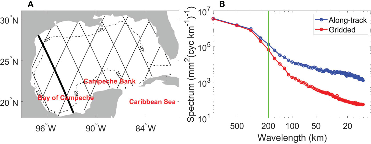
Figure 1 (A) Ground tracks of the TOPEX/Poseidon satellite in the GoM. The thick black line represents the track along which the wavenumber spectrum of ADT was estimated. The dashed black line represents the 200-m isobath. (B) Wavenumber spectrum of along-track and gridded ADT along the track marked by the thick black line in (A). The vertical green line marks the wavelength of 200 km.

ADT data were further processed before they were used to detect eddies. First, since altimetry observations near the coast are less reliable and more than 30% of along-track data are not available for the mapping of the gridded product at locations less than 30 km away from the coast (Saraceno et al., 2008; Castelao and He, 2013), ADT data at grid points that are 30 km or less away from the coast were discarded. However, it should be noted that the quality of altimetry data gets worse in shallower water (Liu et al., 2012). Second, to make eddy features stand out from the large-scale background SSH field, a two-dimensional spatial filter with a cut-off wavelength of 1000 km was applied to the gridded ADT data. The spatial filtering removes the large-scale variability of SSH that is dominated by the seasonal steric height, which is similar to removing the daily spatial average ADT over the deep-water GoM. Third, because the LC has a shape of a loop, which is different from isolated mesoscale eddies but might be recognized as eddy by the eddy detection algorithms, the LC was isolated so that no eddy was considered within the LC. Leben (2005) used the 17-cm contour of ADT to define the LC front. As the mean reference SSH field in this study was different from that used in Leben (2005), we used the 25-cm contour of the SSH anomalies to define the LC front. Because we would like to eliminate the spatially uniform variability of SSH in the GoM, the SSH anomalies with the spatially mean SSH removed were used to find the LC front. The northern boundary of the LC obtained using the 25-cm contour of SSH anomalies shows similar variability as that reported in Leben (2005). Eulerian eddy detection and tracking algorithms were then applied to the high-passed ADT fields.

Other variables were also explored to explain some of the detected eddy characteristics. The global atlas of the first-mode Rossby radius of deformation (Chelton et al., 1998) was used to calculate the standard first-mode Rossby wave propagation velocity, c=-βR², where β is the meridional variation of the Coriolis parameter and R is the first-mode Rossby radius of deformation. Moreover, the multivariate ENSO index (MEI V2) (Zhang et al., 2019), NAO index (Hurrell, 1995), and AMM index (Chiang & Vimont, 2004) were used to examine possible relationships between the eddy activity in the GoM and climate modes.

2.2 Eddy detection and tracking algorithms

An approach that combines three Eulerian eddy detection algorithms proposed by Faghmous et al. (2015); Le Vu et al. (2018), and Halo et al. (2014) was developed to detect Eulerian mesoscale eddies in the GoM. The three algorithms represent different approaches of automatic eddy detection and hereafter are referred to as F15, L18, and H14, respectively. In the F15 algorithm, eddies are defined as features of closed-contour SSH with one extremum of SSH. The eddy center is at the location with extremum SSH. The H14 algorithm combines the OW parameter and geometrical properties of SSH. It identifies eddy as contained within a close loop of SSH and dominated by vorticity with the negative OW parameter. The eddy center is the mean position of the identified eddy. The L18 algorithm is a hybrid method based on physical parameters and geometrical properties of the velocity field. The eddy is contained within closed streamlines around an eddy center with a local maximum normalized angular momentum. The differences between the three eddy detection algorithms are that closed SSH contours are used in F15 and H14, while closed streamlines are used in L18. The eddy center is defined differently in the three algorithms and is associated with the SSH extremum location, mean position of eddy, and the local maximum normalized angular momentum in F15, H14, and L18, respectively.

Due to the limited resolution of the gridded ADT field, a minimum of 9 pixels was used in the F15 algorithm and a minimum eddy radius of 37 km was used in the other two algorithms. The threshold value of nine pixels was selected in the F15 algorithm because it corresponds to a square area that is occupied by the smallest eddy with a radius of 37 km. Also, a minimum eddy amplitude of 2 cm was applied due to the accuracy of the SSH product (Pujol et al., 2016). The three eddy detection algorithms were implemented to the high-passed ADT field, yielding daily mesoscale eddies. An example of the detected eddies on 20 March 1995, as marked by the black circles in Figures 2A-C, shows that some eddies can be detected by one algorithm but cannot be detected by the others. The three algorithms, F15, L18, and H14, gave rise to a total of 67016, 65852, and 55309 anticyclonic eddies (AEs), and a total of 93054, 93118, and 86077 CEs in the GoM over the examined period, respectively. The daily mean area occupied by AEs in F15, L18, and H14 is 1.91e5 km², 2.42e5 km^2, and 9.57e4 km², respectively; while the daily mean area occupied by CEs in F15, L18, and H14 is 2.1e5 km², 2.45e5 km², and 1.14e5 km², respectively. The H14 algorithm yields the smallest eddy size and the least eddy number, suggesting the H14 algorithm is more restrictive than the other two algorithms. Moreover, to examine the influence of the spatial filtering that removes the large-scale variability of SSH on eddy detection, we run the eddy detection algorithms on the unfiltered ADT field and compare the eddy numbers with those from the filtered ADT field. A total of 139867, 148309 and 125886 eddies are found in F15, L18, and H14, respectively, which are less than 158970, 160070 and 141386 eddies when the filtered ADT field is used (Eddy number and area are listed in Table S1 in the supplementary material). The differences of eddy numbers obtained from the filtered and unfiltered ADT fields are from 7% to 12% of the total eddy number. Therefore, the spatial filtering can make eddy features stand out from the large-scale background ADT field.

FIGURE 2

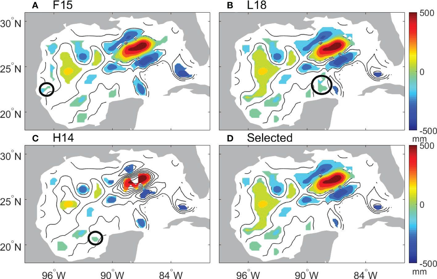
Figure 2 Snapshots of the high-passed ADT (contours) and detected eddies (color shading) on 20 March 1995. Eddies were detected by (A) F15 algorithm, (B) L18 algorithm, (C) H14 algorithm, and (D) eddies were selected by a combination of the three algorithms. The black circle in (A–C) encloses the eddy that was detected by one algorithm but not detected by the other two algorithms.

We focus on the Eulerian mesoscale eddies that can be detected by at least two algorithms. Eddies from the most recently developed L18 algorithm were used as basis eddies. For each basis eddy, if common eddy pixels were found in H14 or F15, the eddy was considered and kept for further processing. There are 10% of AEs and 7% of CEs detected by L18 that were removed based on the comparison of outputs of the three algorithms. Mesoscale eddies are selected in this way so that we have more confidence in the detected eddies than that given by one algorithm, but they are less restrictive than those given by the H14 method. Figures 2A-C show an example of eddies on 20 March 1995 detected by F15 algorithm, L18 algorithm and H14 algorithm, respectively. The black circles in Figures 2A-C enclose the eddy that was detected by one algorithm but not detected by the other two algorithms. An example of selected eddies on 20 March 1995 is shown in Figure 2D, and the selected eddies are those that were detected by at least two algorithms.

The resulting eddies were then tracked with an algorithm that was also used in Le Vu et al. (2018). First, each detected eddy e_i at the last time step t is associated with the closest eddy e_j of the same sign detected at the previous time step t-dt in a given search area. The maximum search distance D_ij is then given by D_ij=C(1 + dt)/2 + <R_max> (j) + R_max(i), where <R_max > (j) is the mean speed-based radius of e_j averaged during the five preceding steps of its track, while R_max (i) is the speed-based radius of e_i(t) that corresponds to the eddy radius with maximum mean azimuthal velocity. The speed parameter C is a constant value of 6.5 km/day that is one typical upper bound of eddy propagation speed used in the maximum search distance D_ij (Le Vu et al., 2018). When no eddies are found in the search area, e_i(t) is identified as a new eddy. When several eddies are found in the search area, e_i will be associated with e_j, which minimizes one cost function:

$${\text{ϵ}}_{ij}=\sqrt{{\left[\frac{d_{ij}}{D_{ij}\left(T_c\right)}\right]}^2+{\left[\frac{\text{Δ}R}{\langle R\rangle \left(j\right)+R\left(i\right)}\right]}^2+{\left[\frac{\text{Δ}Ro}{\langle Ro\rangle \left(j\right)+Ro\left(i\right)}\right]}^2+{\left(\frac{dt}{2T_c}\right)}^2}$$

where d_ij is the distance between e_i and e_j; D_ij(Tc) is the distance D_ij at the correlation time (Tc=10 days); ΔR and ΔRo are the radius and the Rossby number difference between e_i and e_j, respectively; <R> (j) and <Ro> (j) are the mean radius and the mean Rossby number of the eddy e_j averaged during the five preceding steps, respectively; the eddy radius is defined as the radius of the circle equivalent to the eddy area. The dimensionless cost function is used to compare physical similarity between eddy pairs. The terms under the root square represent the relative distance between eddy centers, the relative difference between eddy radius, the relative difference between the intensity characterized by Rossby number and the relative difference of temporal separation, respectively. Eddy merging and splitting due to eddy-eddy interactions are considered in this tracking algorithm. Because the temporal correlation scales of gridded ADT data are about 30 days at latitudes of the GoM (Pujol et al., 2016), only eddies with a lifetime greater than 30 days are examined in this study. Although there are eddies with lifetime shorter than 30 days, the gridded SSH data are not independent on timescales shorter than 30 days and are not sufficient to detect the short-lived eddies.

AEs were further grouped into LCEs and non-LCE AEs. LCEs are AEs that were generated east of 92°W, were dead west of 90°W, translated westward for more than 2 degrees, and had eddy amplitude at the birth time larger than 0.12 m and have a lifespan of more than 60 days. The eddy amplitude was defined as the difference between the SSH on the contour of maximum rotation speed and maximum or minimum SSH in the eddy. Because the LC may experience detachment and reattachment during the formation of LCE, the identified LCE may lose tracking and new eddies were identified. Therefore, AEs that were formed east of 92°W with amplitude larger than 0.2 m and with the distance between eddy center and the LC front being less than 250 km were considered as LCEs as well. The threshold values used in the definition of LCEs were chosen by comparing detected AEs with the SSH maps that show separations of LCEs from the LC. A total of 51 LCE trajectories were found. Among the 35 LCEs with industry names, separation dates of 28 LCEs are less than 1 month different from those reported by Hall and Leben (2016). There are 376 non-LCE AE trajectories. CEs were further grouped into LCFEs and non-LCFE CEs. Based on the CE trajectories, LCFEs are CEs that have the distance between the eddy center and the LC front be less than 200 km in the first 20 days after the generation. LCFEs defined in this way propagate along the LC front during their lifetimes. Non-LCFEs are CEs that are not identified as LCFEs. There are 297 LCFE trajectories and 447 non-LCFE CE trajectories (Number of eddy trajectory is listed in Table S2 in the supplementary material).

3 Results

3.1 Eddy frequency and propagation

Figure 3 shows the percentages of months when eddy birth, death, and presence were observed over the observation period. The months of eddy birth and death were the times when eddies were first and last detected, respectively. LCEs were mostly generated in the northwestern tip of the LC (Figure 3A), were mostly dissipated in the western GoM, and some of them could reach the western boundary of the GoM (Figure 3B). They traveled from the east to the southwest in a broad meridional band, consistent with the broad paths of LCEs revealed in previous studies (e.g., Vukovich and Crissman, 1986; Hamilton et al., 1999; Vukovich, 2007). Therefore, it is more frequent to observe LCEs in the band from the east to the southwest (Figure 3C).

FIGURE 3

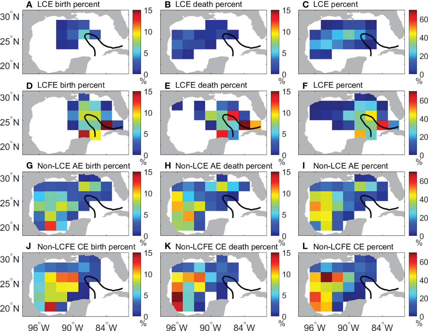
Figure 3 (A, D, G, J) The percentage of months when eddy birth was observed from January 1993 to April 2019. (B, E, H, K) The percentage of months when eddy death was observed. (C, F, I, L) The percentage of months when the presence of eddy was observed. LCEs, LCFEs, non-LCE AEs, non-LCFE CEs are shown in (A-C), (D-F), (G-I), and (J-L), respectively. The black line represents the 25-cm contour of temporal mean SSH anomalies from 1993 to 2019.

LCFEs were mostly generated east of Campeche Bank, in the northern and eastern LC (Figure 3D), and they were more likely to dissipate in the eastern LC (Figure 3E). LCFEs traveled mainly in the eastern GoM because they were closely tied to the LC. LCFEs generated around the Campeche Bank did not travel or lost tracks along the western part of the LC. In the eastern part of the LC, LCFEs traveled along the southward flowing LC. These are consistent with the previous conclusion that LCFE motions along the northern and eastern LC were decoupled from the LCFE motions along the southwestern LC (Walker et al., 2009; Donohue et al., 2016a; Donohue et al., 2016b; Hamilton et al., 2016). LCFEs were most frequently found east of Campeche Bank and in the eastern LC (Figure 3F). A large fraction of LCFEs has been reported on the eastern flank of the Campeche Bank (Zavala-Hidalgo et al., 2003; Le Hénaff et al., 2014; Jouanno et al., 2016).

In contrast to the LCEs and LCFEs that were directly related to the instability of the LC in the eastern GoM, non-LCE AEs and non-LCFE CEs were mostly generated in the western GoM, especially in the central-western GoM and in the Bay of Campeche (Figures 3G, J). They were prone to dissipate along the western boundary of the GoM (Figures 3H, K). The non-LCE AEs and non-LCFE CEs are mostly in the western GoM and do not affect the eastern GoM. The presence frequencies of these eddies are also the highest west of 92°W (Figures 3I, L).

Although dynamic instabilities of large-scale currents have been reported to be important for the aforementioned spatial pattern of eddy generation (e.g., Sturges and Leben, 2000; Zavala-Hidalgo et al., 2003; Chérubin et al., 2006; Donohue et al., 2016a; Jouanno et al., 2016; Maslo et al., 2020; Yang et al., 2020), the eddy-topography interaction and eddy-eddy interaction could play a role in generating new eddies (Smith and David, 1986; Vidal et al., 1992; Biggs et al., 1996; Frolov et al., 2004). The eddy-eddy interaction including eddy splitting and merging was also considered in this study following Le Vu et al. (2018). When a characteristic shared contour encloses two eddy centers and the mean velocity along the shared contour reaches a maximum value larger than the maximum velocity of at least one eddy, the two eddies inside the shared contour experience eddy interaction. If such a characteristic shared contour is detected and there is only one trajectory before the eddy interaction period, a splitting event is considered. New eddies due to splitting accounts for 15.4% of the total generated eddies. Only 2 LCEs and 16 LCFEs were generated by splitting. However, 80 non-LCE AEs and 82 non-LCFE CEs were generated by splitting and account for 7% of the total generated eddies, respectively. Most non-LCE AEs and non-LCFE CEs due to eddy splitting were scattered in the western GoM (Figure 4A). In addition to eddy splitting, LCEs could induce eddies along their periphery during the traveling period because of the relatively large current shear around LCEs or when they encounter the western boundary of the GoM. Figure 4B shows the center locations of eddies that were generated along LCE periphery. There are 14 non-LCE AEs and 118 non-LCFE CEs (10% of the total generated eddies) that are likely related to LCEs, showing no particular pattern. Only a small number of CEs were generated along the western boundary of GoM as LCEs arrived there, suggesting that the interaction between LCEs and topography plays a relatively small role in creating new eddies. The dominance of CEs that are possibly induced by LCEs is consistent with the fact that the current shear along LCE periphery is mainly cyclonic.

FIGURE 4

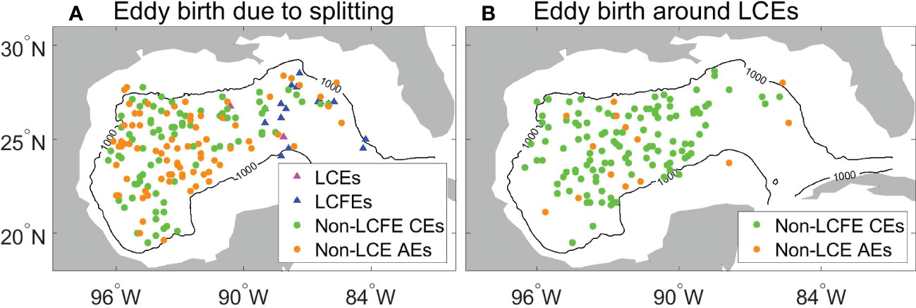
Figure 4 (A) Locations of generated eddies due to splitting. (B) Locations of generated eddies within LCE radius plus 100 km.

Moreover, eddy propagation velocities were estimated by least-squares fitting the positions of eddy centers as a function of time in overlapping 30-day segments of each eddy’s trajectory. Figure 5 shows the mean eddy propagation speeds and directions. Mean eddy propagating speeds are highly variable in the GoM. Specifically, LCEs have large traveling speeds in the central-western GoM that can be as large as 5 km/day (Figure 5A). The mean propagating direction of LCEs is southwestward in the central GoM and bifurcates north and south when LCEs encounter the western boundary of GoM. LCFEs propagate along the LC front and large propagation speeds are found in the eastern part of the LC (Figure 5B) that are related to the advection of the LC. Non-LCE AEs and non-LCFE CEs have large propagation speeds in the southwest of the GoM and the dominant propagation direction of the two types of eddies is to the west (Figures 5C, D). The eddy speeds in the western GoM have a similar magnitude as the first-mode Rossby wave propagation speeds (Chelton et al., 2011). However, it should be noted that eddy speeds larger than the first-mode Rossby wave propagation speeds by more than 1 km day^-1 were also found, which might be related to the background circulation, or in the case of CEs caused by the swirl velocities of a large LCE.

FIGURE 5

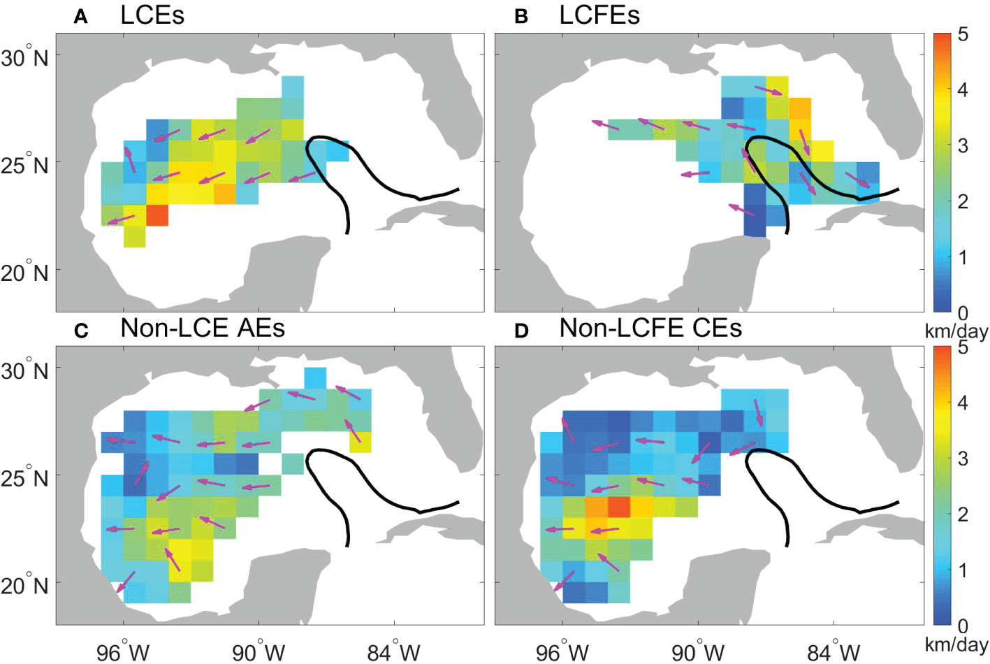
Figure 5 Mean eddy propagation speeds (color shading) and directions (magenta arrows) for (A) LCEs, (B) LCFEs, (C) non-LCE AEs, and (D) non-LCFE CEs. The thick black line represents the 25-cm contour of temporal mean SSH anomalies from 1993 to 2019.

3.2 Basic eddy characteristics

Distributions of some basic eddy characteristics derived from the mean values along eddy trajectories are presented in Figures 6A-D, and the distribution of eddy lifetime is shown in Figure 6E. Apparent differences between the four types of eddies appear in their amplitude, scale, relative vorticity, and maximum rotational speed (Figures 6A-D). LCEs have the largest mode values of eddy amplitude, LCFEs have a smaller eddy amplitude, and non-LCE AEs and non-LCFE CEs have the smallest mode values of eddy amplitude (Figure 6A). The distributions of the eddy scale, defined as the radius with the maximum rotational speed (Chelton et al., 2011), show that LCEs have the largest scale and that the other three types of eddies have smaller and similar mode values of eddy scale (Figure 6B). The distributions of the relative vorticity, and maximum rotational speed show that LCEs and LCFEs have larger magnitudes of mode values than those of non-LCE AEs and non-LCFE CEs (Figures 6C, D). Nearly 25.1% of AEs have a lifetime longer than 100 days. About 16.7% of CEs can live longer than 100 days (Figure 6F).

FIGURE 6

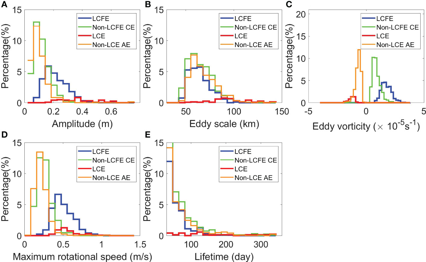
Figure 6 Histograms of basic eddy characteristics: (A) amplitude (m), (B) eddy scale (km), (C) eddy relative vorticity (s^-1), (D) maximum rotational speed (m/s), (E) lifetime (day).

Because the temporal correlation scale of gridded ADT data is about 30 days, the obtained eddy amplitude, scale, and maximum rotational speed were mapped into monthly data on two-degree grids. To illustrate their spatial distributions, the temporal mean eddy characteristics on spatial grids are shown in Figure 7. Eddy characteristics within the LC are not considered in this study because SSH fields within the LC region were removed. Mean values of the LCE amplitude, scale, and maximum rotational speed are large northwest of the LC where LCEs were shed from the LC (Figures 7A-C) and are much larger than those of the other three types of eddies. The larger amplitude of LCEs is expected due to their larger size even with a rotational speed comparable to smaller eddies. LCFEs have relatively large amplitude and rotational speed in the southeastern part of the LC (Figures 7D, F), in agreement with previous estimates that LCFEs have larger amplitude and rotational speed in the northern and eastern side of the LC than on the western side (e.g., Le Hénaff et al., 2014). Compared to the eddy amplitude and rotational speed, the LCFE scale is relatively uniform (Figure 7E). In contrast to LCEs and LCFEs, non-LCE AEs and non-LCFE CEs show relatively small spatial variations of amplitude, scale, and rotational speed (Figures 7G-L). The spatial patterns of the eddy amplitude, scale, and maximum rotational speed are not likely related to the eddy number distributions (Figures 3, Figure 7).

FIGURE 7

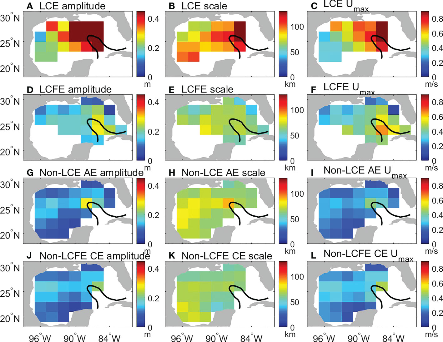
Figure 7 Eddy mean amplitude (m) for (A) LCEs, (D) LCFEs, (G) non-LCE AEs, and (J) non-LCFE CEs. Eddy mean scale (km) for (B) LCEs, (E) LCFEs, (H) non-LCE AEs, and (K) non-LCFE CEs. Eddy mean maximum rotational speed (m/s) for (C) LCEs, (F) LCFEs, (I) non-LCE AEs, and (L) non-LCFE CEs. The black line represents the 25-cm contour of temporal mean SSH anomalies from 1993 to 2019.

3.3 Monthly climatology of eddies

Monthly climatology of eddy number was obtained and expressed in percentage of the total generated eddies (Figure 8). The seasonal peak of LCE birth in September and the secondary peak in February are observed (Figure 8A), which are consistent with that reported by Hall and Leben (2016). The seasonal variation of LCEs is the smallest compared to the other three types of eddies and is not significant at the 95% confidence level. The nonsignificant seasonal variability of LCE separation may be partially related to the physical processes that do not have apparent seasonal variability but can affect the LCE separation. For example, fluctuations such as mesoscale eddies from the Caribbean Sea (Murphy et al., 1999; Oey et al., 2003; Huang et al., 2021) can influence the LCE separation.

FIGURE 8

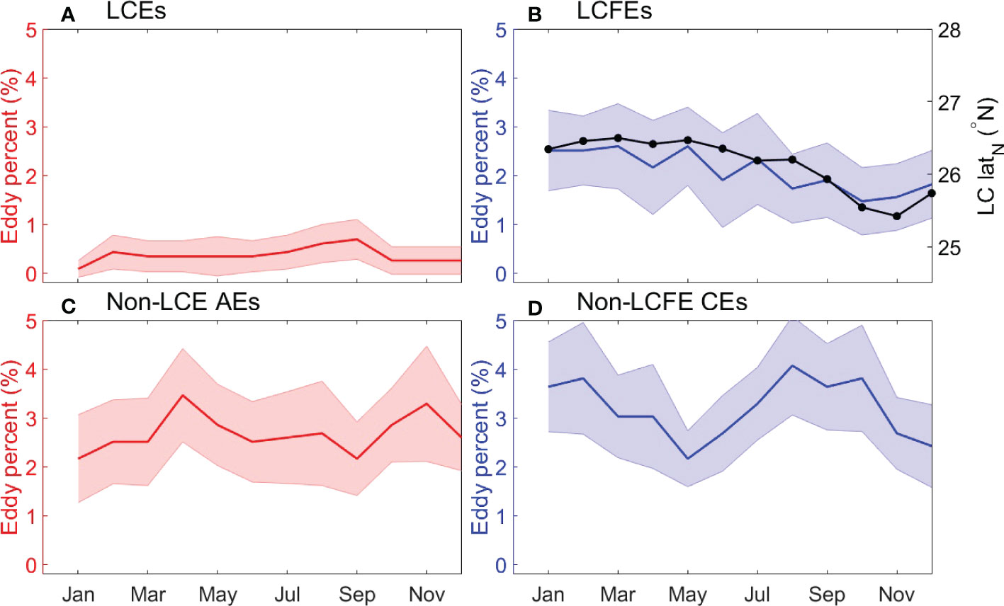
Figure 8 (A) The percentage of birth number of LCEs relative to the total eddy birth number. (B) The percentage of birth number of LCFEs relative to the total birth number. The black line in (B) represents the monthly climatology of the LC position. (C) The percentage of birth number of non-LCE AEs relative to the total birth number. (D) The percentage of birth number of non-LCFE CEs relative to the total birth number. The shading denotes the 95% confidence level represented by two times standard deviation of eddy percentage in each month.

Compared to LCEs, more LCFEs are observed and the birth number of LCFEs is larger in January to July than in October to December (Figure 8B). The magnitude of the seasonal variation of LCFEs is close to 1% of the total eddy birth number, but it is still not significant at the 95% confidence level. Because LCFEs are generated along the LC peripheral, the extent of northern penetration of the LC may be one important factor for the LCFE generation. The seasonal variation of the northern boundary of the LC is shown to have a similar variation as that of LCFEs (Figure 8B). Hamilton et al. (2014) also showed that altimeter-derived LC northern-boundary latitude is relatively high from January through about July and low in September and October. The more northward the LC penetrates, the more LCFEs are generated.

The seasonal variations of non-LCE AEs and non-LCFE CEs are relatively large, but differences of eddy number between most months are not significant at the 95% confidence level due to large uncertainties (Figures 8C, D). The number of non-LCFE CEs is small in May and December and is large in February and August (Figure 8D), indicating a biannual variability. Compared to the non-LCFE CEs, the seasonal variation of non-LCE AEs has a different phase and a smaller amplitude (Figure 8C). Both the background currents and eddy-eddy interaction might be important for the seasonality of the two types of eddies. Figure 9 shows the monthly climatology of the eddy numbers of non-LCE AEs and non-LCFE CEs that were induced by eddy splitting and LCEs. The seasonal variations of AEs and CEs induced by splitting and LCEs are small and are not significant at the 95% confidence level. It should be noted that their seasonal variations are much smaller and more random than those shown in Figures 8C, D. Therefore, the seasonal variations of non-LCE AEs and non-LCFE CEs (Figures 8C, D) are not related to eddy-eddy interaction represented by eddy splitting and the effect of LCEs and could be likely related to the background currents. It is noted that the seasonal variations of the eddies are not robust. The large uncertainties of the seasonal variations of eddies are likely related to the multiple factors that can influence the large-scale background circulation such as the LC. In the eastern GoM, the seasonal variability of the LC can be modulated both by wind forcing over the northwestern Caribbean Sea and GoM (Chang and Oey, 2012; Chang and Oey, 2013) and by mesoscale variability in the Caribbean Sea (Murphy et al., 1999; Oey et al., 2003). In the western GoM, both the irregular LCEs and seasonal wind forcing contribute to the circulation that is partially important for the eddy generation (e.g., Sturges, 1993).

FIGURE 9

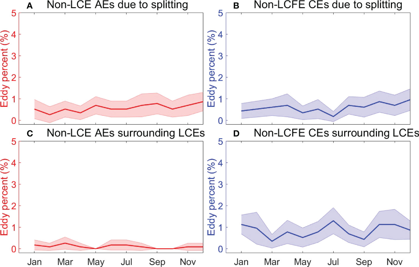
Figure 9 (A) The percentage of non-LCE AEs generated due to splitting relative to the total generated eddies. (B) The percentage of non-LCFE CEs generated due to splitting relative to the total generated eddies. (C) The percentage of non-LCE AEs generated within LCE radius plus 100 km relative to the total generated eddies. (D) The percentage of non-LCFE CEs generated within LCE radius plus 100 km relative to the total generated eddies. The shading denotes the 95% confidence level represented by two times standard deviation of eddy percentage in each month.

To further show spatial patterns of the monthly climatology of generated eddies, the locations of eddy centers were mapped on two-degree grids (Figure 10). Figures 10A-D shows the generation locations of LCEs and the mean position of the LC in February, May, August, and November (the generation locations of LCEs in 12 months are shown in Figure S1 in the supplementary material). The LC has a more northward penetration in February and May than in August and November but more LCEs are formed at the northwestern tip of the LC in August than in other months, suggesting no clear linkage between the generation of LCEs and the LC northern boundary can be built. However, more LCFEs can be found in the northern LC in February and May when the LC makes more penetration than in August and November when the LC makes less penetration (Figures 10E-H) (the generation locations of LCFEs in 12 months are shown in Figure S2 in the supplementary material). Therefore, a more northward penetration of the LC favors the generation of LCFEs.

FIGURE 10

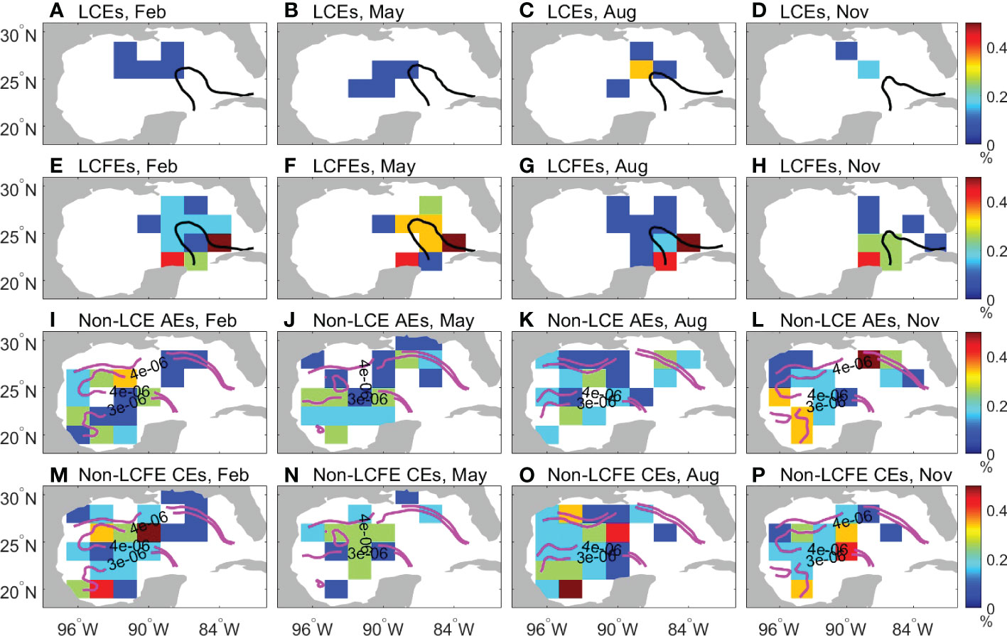
Figure 10 (A-D) LCE percentage relative to the total generated eddies in (A) February, (B) May, (C) August, and (D) November. (E-H) LCFE percentage relative to the total generated eddies in (E) February, (F) May, (G) August, and (H) November. (I-L) Non-LCE AE percentage relative to the total generated eddies in (I) February, (J) May, (K) August, and (L) November. (M-P) Non-LCFE CE percentage relative to the total generated eddies in (M) February, (N) May, (O) August, and (P) November. The black lines in (A-H) represent the mean position of the LC in February, May, August, and November, respectively. The magenta lines in (I-P) represent the monthly climatology of current speed gradient in February, May, August, and November, respectively.

Compared to LCEs and LCFEs that are closely related to the LC, the generation of non-LCE AEs and non-LCFE CEs is scattered over the whole GoM and is mainly in the western GoM (Figures 10I-P) (the generation locations of non-LCE AEs and non-LCFE CEs in 12 months are shown in Figures S3 and S4 in the supplementary material). The contours of current speed gradient in Figures 10I-P indicate the position of strong background currents. The generation locations of eddies tend to move with the seasonal movement of strong currents, from which eddies may obtain energy. However, non-LCE AEs do not show a significant change in the birth number between different months, which is also indicated in Figure 8C. It is noted that the number of non-LCFE CEs is more likely related to the strength of the background currents (Figures 10M-P). More non-LCFE CEs were generated along the boundary of strong currents in February and August and fewer non-LCFE CEs were generated in May and November. The current speeds and directions in the four months are highlighted and shown in Figure 11 (the current speeds and directions are shown in Figure S5 in the supplementary material). The background currents in western GoM are stronger in February and August than in May. The mean currents in the central western GoM flow westward approximately at 22-23°N and eastward at 25-27°N, forming an anticyclonic circulation pattern. It is noted that the currents change direction with season along the western boundary. Therefore, the non-LCFE CEs were more likely formed along the periphery of the strong anticyclonic circulation pattern in the western GoM. It is noted that the eddy generation location varies within the strong-current region and sometimes few eddies are generated. One possible reason is that the large-scale background current can influence the eddy generation but is not the only factor that determines the eddy generation location and other factors such as wind stress play some role.

FIGURE 11

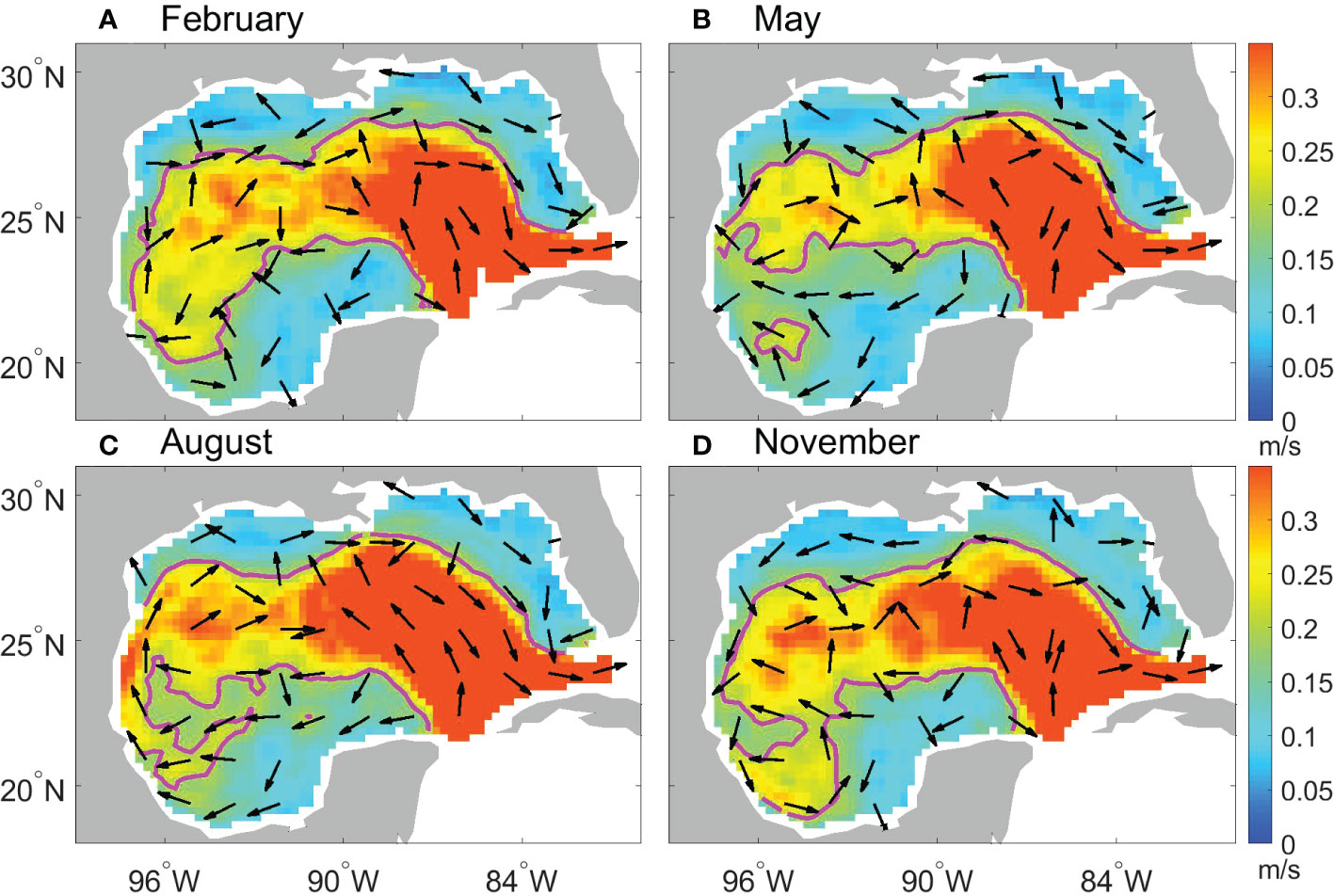
Figure 11 Current speeds (m/s, color shading) climatology and mean current direction (arrows) in the GoM in (A) February, (B) May, (C) August, and (D) November. The magenta contour denotes the current speed of 0.2 m/s.

In addition to the seasonality observed in the eddy birth number, the seasonal variability of eddy amplitude at the time of eddy birth was examined. The monthly climatology of median eddy amplitude is presented in Figure 12. Since eddy amplitude is not normally distributed, median eddy amplitude was used to mitigate the potential influence of amplitude outliers. Compared to the seasonal variability of eddy number, the seasonal variability of eddy amplitude is less apparent. This is because eddy amplitude is defined as the difference between the SSH on the contour of maximum rotation speed and maximum or minimum SSH in the eddy. In the LCEs and LCFEs region, SSH variations are dominated by intra-seasonal oscillations, not by annual cycles or seasonal variations (Liu et al., 2016; Weisberg et al., 2017). LCEs and LCFEs have relatively larger monthly variations and uncertainties than non-LCE AEs and non-LCFE CEs. It should be noted that the seasonal variation of LCE amplitude may not be reflected from the relatively short record because it was estimated from a relatively small number of LCEs that is less than 6 in most months.

FIGURE 12

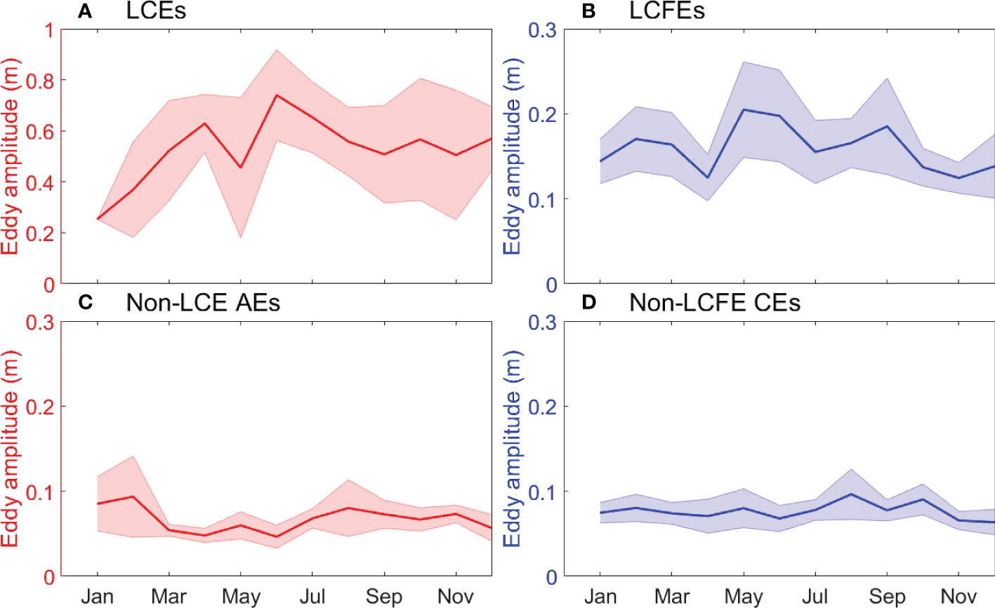
Figure 12 Monthly climatology of eddy amplitude of (A) LCEs, (B) LCFEs, (C) non-LCE AEs, and (D) non-LCFE CEs whey they were generated. The shading denotes the 95% confidence level represented by two times standard deviation of amplitude.

3.4 Low-frequency variability of eddies

To examine the low-frequency variability of eddies, annual variations of eddy birth number and amplitude were obtained. Figure 13 shows the annual variations of the birth number of eddies. The generation of LCEs is relatively rare and shows a weak variability (Figure 13A). The other three types of eddies indicate a larger variability. A linear regression model that includes a linear trend, ENSO index, NAO index, and AMM index was applied to the annual eddy number. An increasing number of LCEs over 2001-2010 has been found in previous studies (Vukovich, 2012; Lindo-Atichati et al., 2013). Nevertheless, no long-term variability of other types of eddies has been reported. The linear trends of the annual birth number of LCEs, LCFEs, non-LCE AEs, and non-LCFE CEs from 1993 to 2018 are 3.5×10^-2 ± 3.3×10^-2 ( ± 1σ) year^-1, -0.2 ± 0.17 ( ± 1σ) year^-1, -0.06 ± 0.11 ( ± 1σ) year^-1, and 0.05 ± 0.11 ( ± 1σ) year^-1, respectively. These linear trends are not significant at the 95% confidence level. LCFEs have the largest decreasing trend that is not significant, which is likely related to the negative trend of the northern boundary of the LC that is -1.7×10^-2 ± 1.7×10^-2 ( ± 1σ) degree year^-1. Regression coefficients of the three climate indices are not significant as well. For the four types of eddies, the coefficients of determination of the three climate indices are less than 0.08. Therefore, only a small portion of eddy number variance can be explained by the three climate modes, indicating that the role of the remote climate variability in changing the eddy activity in the GoM is relatively small or cannot be detected from the linear model.

FIGURE 13

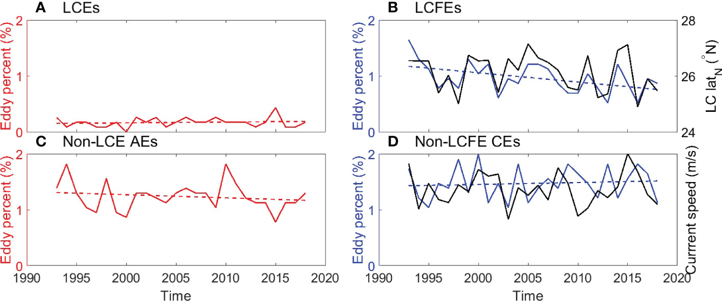
Figure 13 Annual number of generated (A) LCEs, (B) LCFEs, (C) non-LCE AEs and (D) non-LCFE CEs and is expressed as percentage of the total new eddy from 1993 to 2018. The black line represents the annual mean northern boundary (°N) of the LC in (B) and the annual mean current speed (m/s) in the western GoM in (D). The dashed lines represent linear trend of generated eddies.

In the eastern GoM, the low-frequency variability of eddy number is likely related to that of the LC. Figure 13B shows the annual mean variation of the northern boundary position of the LC that particularly follows the variation of LCFEs. Correlation between the birth number of LCEs and the northern boundary position of the LC is small and not significant (Correlation coefficient r=0.38), therefore, the extent of LC penetration plays a relatively small role in the separation of LCEs. However, the LCFE number and the northern boundary position of the LC are correlated with a significant correlation coefficient of 0.76, indicating that the LCFE number increases with the northward penetration of the LC on the interannual to multidecadal time scale. The extent of northward penetration of the LC is important for the LCFE generation although previous studies have shown that perturbations coming from the Caribbean Sea (Huang et al., 2013) and the topography of the northern Campeche (Chérubin et al., 2006) also contribute to the eddy activity along the western edge of the LC.

For the non-LCE AEs and non-LCFE CEs, the eddy numbers also show large annual mean variations (Figures 13C, D). Since the background current strength could be important in affecting the low-frequency eddy activity (Chen et al., 2011), birth numbers of non-LCE AEs and non-LCFE CEs, which were mostly formed in the western GoM, were compared with the surface current speed averaged in the western GoM (Figure 13D). The non-LCE AE number is anticorrelated with the mean surface current speed in the western GoM (r=-0.42). The non-LCFE CE number is correlated with the mean surface current speed in the western GoM (r=0.33). But the correlation values are not significant at the 95% confidence level.

In addition to the influence of background currents, the eddy-eddy interaction that includes eddy splitting and eddy formation related to LCEs is considered as well. The annual mean variability of eddies due to eddy-eddy interaction is relatively weak. After removing the eddies induced by eddy splitting and LCEs, the correlations between non-LCE AE number, non-LCFE CE number, and the mean surface current speed in the western GoM are -0.38 and 0.32, respectively. The eddy-eddy interaction has little effect on the relationship between western eddies and the background flows. Since a much smaller number of eddies due to eddy splitting and LCEs are found along the western boundary (Figure 4) where LCEs could interact with the topography (e.g., Vidal et al., 1992), the eddy-topography interaction is not important for the low-frequency variability of eddies.

The relationship between the eddy number and the strength of the circulation in the western GoM was further examined with composite analysis. The mean current speeds and flow directions during the periods with more non-LCFE CEs and fewer non-LCFE CEs are shown in Figure 14. When the annual number of non-LCFE CEs is one standard deviation larger than the average eddy number, strong mean anticyclonic circulation is observed in the western GoM. When the annual number of non-LCFE CEs is one standard deviation smaller than the average eddy number, weak mean anticyclonic circulation is observed in the western GoM. However, over the period with more non-LCE AEs weak mean anticyclonic circulation is observed in the western GoM. Over the period with fewer non-LCE AEs strong mean anticyclonic circulation is observed in the western GoM. Therefore, the strength of the background circulation could play a role in influencing the low-frequency variability of eddy number.

FIGURE 14

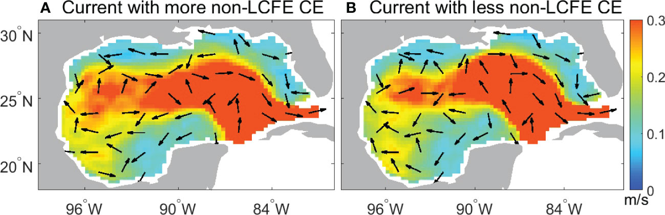
Figure 14 Composite of current speeds in the GoM (A) during the period with more generated non-LCFE CEs (annual number of non-LCFE CEs is larger than mean value plus one standard deviation), and (B) during the period with fewer non-LCFE CEs (annual number of non-LCFE CEs is smaller than mean value minus one standard deviation). Arrows denote the mean current direction.

Eddy amplitude in the GoM exhibits low-frequency variability as well. To mitigate the potential influence of amplitude outliers, the median amplitude of eddies at the time of birth in each year was selected for the analysis of the low-frequency variability of eddy amplitude (Figure 15). LCEs show the largest annual variation of eddy amplitude (Figure 15A) that was obtained from a small number of LCEs (Figure 13A). The amplitude variation of LCFEs is weaker than that of LCEs but is larger than those of non-LCE AEs and non-LCFE CEs (Figure 15B). The variations of LCE and LCFE amplitude are not closely related to the northern boundary of the LC with small correlations, suggesting the extent of the LC penetration is not an important factor for the eddy amplitude at the time of birth. For non-LCE AEs and non-LCFE CEs, the eddy amplitude at the time of birth seems to be related to the strength of background currents in the western GoM (Figures 15C, D) but with a nonsignificant positive correlation of 0.47.

FIGURE 15

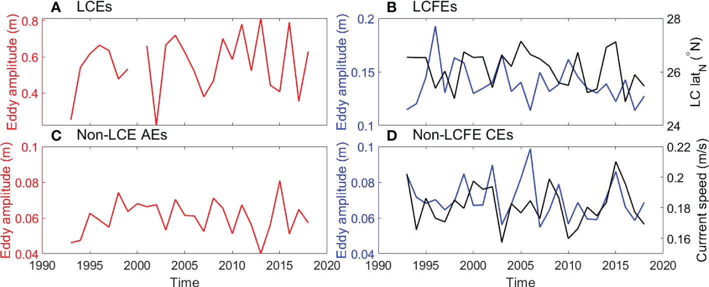
Figure 15 Annual median amplitude (m) of the (A) LCEs, (B) LCFEs, (C) non-LCE AEs and (D) non-LCFE CEs when they were generated. The black line represents the annual mean northern boundary (°N) of the LC in (B) and the annual mean current speed (m/s) in the western GoM in (D).

4 Conclusions and discussions

In this study, we present characteristics of the Eulerian mesoscale eddies in the GoM, including their spatial distributions, seasonal and low-frequency variabilities. As expected, many eddy characteristics in the eastern GoM are closely related to the LC, which sheds large and strong LCEs and develops small-scale LCFEs (e.g., Le Hénaff et al., 2014; Brokaw et al., 2020). Compared to LCEs and LCFEs, non-LCE AEs and non-LCFE CEs are mainly formed in the central-western GoM, tend to dissipate along the western boundary, and have smaller amplitude, relative vorticity magnitude, and rotational speed. Temporally mean propagation speeds are high in the eastern part of the LC and the southwestern GoM.

The temporal variability of eddy occurrence and amplitude, which is less reported in the literature, shows manifest spatial patterns and dramatic differences between LCEs, LCFEs, non-LCE AEs, and non-LCFE CEs. This study indicates a biannual variability of LCE separation with large uncertainties that is similar to that found in a shorter record by Hall and Leben (2016). However, the seasonality in LCE formation is not significant, while Hall and Leben (2016) suggested that the seasonal peak in LC eddy separation events in August and September was significant. The seasonal variabilities of birth numbers of the other three types of eddies are also not significant at the 95% confidence level. Nevertheless, LCFEs and non-LCFE CEs show more apparent seasonal patterns than LCEs and non-LCE AEs. More LCFEs are observed from January to July, while more non-LCFE CEs are found in February and August. Fewer LCFEs are observed from August to December, while fewer non-LCFE CEs are found in May and December. Moreover, the seasonal variability of eddy amplitude at the time of eddy birth is more random than that of eddy number. Similar to the temporal mean characteristics, the seasonal variability of eddy amplitude of LCEs and LCFEs at the time of eddy birth is much larger than that of non-LCE AEs and non-LCFE CEs. On the low-frequency time scale, although an increasing number of LCEs in the decade 2001-2010 has been found in previous studies (Vukovich, 2012; Lindo-Atichati et al., 2013), the linear trends of LCEs and other three types of eddies obtained in this study are not significant at the 95% confidence level.

The seasonal and low-frequency variabilities described above could be closely related to the large-scale background circulations such as the LC, eddy-eddy interaction, and eddy-topography interaction. On the seasonal time scale, the extent of northward penetration of the LC is important for LCFE generation but not for their amplitude. The position and strength of background currents in the western GoM are likely important for the formation of non-LCFE CEs and non-LCE AEs that are mostly formed in the western GoM. On the low-frequency band (interannual to multidecadal), LCFE number is related to the extent of northward penetration of the LC in the eastern GoM. In the western GoM, the surface circulation strength could be important for the low-frequency variability of eddy occurrence and amplitude, which is also found in other oceans (e.g., Chen et al., 2011). In contrast, the eddy-eddy interaction that includes eddy splitting and the effect of LCEs and the eddy-topography interaction give rise to a relatively small number of eddies and play a small role in the temporal variability of eddies.

Note that the Eulerian eddies examined in this study are interpreted as mesoscale perturbations with closely SSH or streamlines, which reflect the generation, propagation, and dissipation of these signals rather than coherent mass. The characteristics of these Eulerian eddies are useful information for the description of the upper-ocean mesoscale variabilities that possess different temperature and salinity and that may exert significant influence on the bottom currents (Brokaw et al., 2020; Zhu and Liang, 2020). Nevertheless, the Eulerian eddies were detected without considering the conservation of material within them. The material within the eddy might exchange with the ambient fluid and might be different during the propagation process. Therefore, the detected and traced eddies examined in this study cannot be directly used to infer the transport of ocean mass, temperature, salinity, and other materials. In cases of examining ocean material transport within mesoscale eddies, Lagrangian methods that consider the conservation of boundary materials should be used (e.g., Andrade-Canto et al., 2020). The Lagrangian coherent vortex is different from the Eulerian eddies in the objective definition of coherent structure that is frame-independent and observer-independent. Eddy characteristics based on the Lagrangian methods can be done and compared with the results obtained with the Eulerian methods in our future work.

In addition to the limitation of eddy detection and tracking algorithms, satellite sampling could affect the detection of the mesoscale activity (Le Traon and Dibarboure, 1999) and the LC statistics (Dukhovskoy et al., 2015). The allsat ADT product was derived from a varying number of altimeters and was useful for examining the influence of satellite sampling on eddy detection. Mesoscale eddies were detected with the algorithm developed by Le Vu et al. (2018) from the allsat ADT product and were compared with those detected from the twosat ADT. From 1 January 1993 to 31 December 1999 when twosat and allsat ADT data were mainly derived from 2 altimeters, 41388 and 41343 eddies were detected from the twosat and allsat ADT data respectively, suggesting that 0.1% of eddies was not detected in allsat ADT. From 1 January 2000 to 13 May 2019 when the allsat ADT data were mainly derived from 3 or more altimeters, 117582 and 117359 eddies were detected from the twosat and allsat ADT data respectively, suggesting that 0.2% of eddies was less detected in allsat ADT than in twosat ADT. The satellite sampling has a relatively small effect on the detection of eddies in the GoM.

In this study, we focus on describing the characteristics of the Eulerian mesoscale eddies in the GoM, and some characteristics such as the temporal and spatial patterns of eddies still need further dynamical explanations. Previous studies indicate that mesoscale eddies in the eastern GoM likely arise from dynamic instabilities, such as barotropic and baroclinic instabilities (e.g., Vukovich and Maul, 1985; Pichevin and Nof, 1997; Sturges and Leben, 2000; Zavala-Hidalgo et al., 2003; Chérubin et al., 2006; Donohue et al., 2016a; Yang et al., 2020). In the future, dynamic analyses such as eddy energy may shed light on the detailed mechanisms of the temporal and spatial variability of mesoscale eddies in the GoM.

Data availability statement

Publicly available datasets were analyzed in this study. This data can be found here: The daily DT2018 ADT data (Taburet et al., 2019) from two altimeter satellites used for eddy detection was provided by the C3S (https://cds.climate.copernicus.eu/cdsapp#!/dataset/satellite-sea-level-global?tab=form). Besides, the daily DT2018 ADT data from multi-mission altimeter satellites used to examine the influence of satellite sampling on eddy detection is SEALEVEL_GLO_PHY_L4_REP_OBSERVATIONS_008_047 that was produced and provided by CMEMS (https://resources.marine.copernicus.eu/product-detail/SEALEVEL_GLO_PHY_L4_MY_008_047/INFORMATION). TOPEX/Poseidon (T/P) along-track ADT data from 2 January 1996 to 3 December 1999 were used to examine the effective spatial resolution of the gridded ADT product in the GoM and were provided by CMEMS. Since the eddy traveling speeds were compared with the first-mode baroclinic Rossby wave speeds, the atlas of the first-baroclinic Rossby radius of deformation was also used and downloaded at https://ceoas.oregonstate.edu/rossby_radius (Chelton et al., 1998). The multivariate ENSO index (MEI V2) (e.g., Zhang et al., 2019) from National Oceanic and Atmospheric Administration (NOAA) Physical Sciences Laboratory, NAO index (Hurrell, 1995) from NOAA Climate Prediction Center, and AMM index (Chiang and Vimont, 2004) from University of Wisconsin were used to examine possible relationships between the eddy activity in the GoM and climate modes. The MEI, NAO index, and AMM index were downloaded at https://psl.noaa.gov/data/climateindices/list/.

Author contributions

YZ and XL designed the experiments and YZ carried them out. YZ prepared the manuscript with contributions from XL. All authors contributed to the article and approved the submitted version.

Funding

The work was supported in part by the National Aeronautics and Space Administration through Grant 80NSSC20K0757.

Acknowledgments

The preprint of the work was submitted for public discussion online (Zhu and Liang, 2022) and the authors acknowledge comments from two reviewers and Dr. Francisco Beron-Vera. The authors thank three reviewers for their constructive comments and suggestions.

Conflict of interest

The authors declare that the research was conducted in the absence of any commercial or financial relationships that could be construed as a potential conflict of interest.

Publisher’s note

All claims expressed in this article are solely those of the authors and do not necessarily represent those of their affiliated organizations, or those of the publisher, the editors and the reviewers. Any product that may be evaluated in this article, or claim that may be made by its manufacturer, is not guaranteed or endorsed by the publisher.

Supplementary material

The Supplementary Material for this article can be found online at: https://www.frontiersin.org/articles/10.3389/fmars.2022.1087060/full#supplementary-material

References

Alvera-Azcárate A., Barth A., Weisberg R. H. (2009). The surface circulation of the Caribbean Sea and the gulf of Mexico as inferred from satellite altimetry. J. Phys. Oceanogr. 39 (3), 640–657. doi: 10.1175/2008JPO3765.1

CrossRef Full Text | Google Scholar

Amores A., Jordà G., Arsouze T., Le Sommer J. (2018). Up to what extent can we characterize ocean eddies using present-day gridded altimetric products? J. Geophysical Res.: Oceans 123, 7220–7236. doi: 10.1029/2018JC014140

CrossRef Full Text | Google Scholar

Andrade-Canto F., Beron-Vera F. J. (2022). Do eddies connect the tropical Atlantic ocean and the gulf of Mexico? Geophysical Res. Lett., 49, e2022GL099637. doi: 10.1029/2022GL099637

CrossRef Full Text | Google Scholar

Andrade-Canto F., Beron-Vera F. J., Goni G. J., Karrasch D., Olascoaga M. J., Triñanes J. (2022). Carriers of sargassum and mechanism for coastal inundation in the Caribbean Sea. Phys. Fluids 34 (1), 016602. doi: 10.1063/5.0079055

CrossRef Full Text | Google Scholar

Andrade-Canto F., Karrasch D., Beron-Vera F. J. (2020). Genesis, evolution, and apocalypse of loop current rings. Phys. Fluids 32 (11), 116603. doi: 10.1063/5.0030094

CrossRef Full Text | Google Scholar

Bello-Fuentes J., García-Nava F., Andrade-Canto H. F., Durazo R., Castro R., Yarbuh I. (2021). Retention time and transport potential of eddies in the northwestern gulf of Mexico. Cienc. Marinas 47 (2):71–88. doi: 10.7773/cm.v47i2.3116

CrossRef Full Text | Google Scholar

Biggs D. C., Fargion G. S., Hamilton P., Leben R. R. (1996). Cleavage of a gulf of mexico loop current eddy by a deep water cyclone. J. Geophysical Res.: Oceans 101 (C9), 20629–20641. doi: 10.1029/96JC01078

CrossRef Full Text | Google Scholar

Bosart L. F., Bracken W. E., Molinari J., Velden C. S., Black P. G. (2000). Environmental influences on the rapid intensification of hurricane opal (1995) over the gulf of Mexico. Monthly Weather Rev. 128 (2), 322–352. doi: 10.1175/1520-0493(2000)128<0322:EIOTRI>2.0.CO;2

CrossRef Full Text | Google Scholar

Brokaw R. J., Subrahmanyam B., Morey S. L. (2019). Loop current and eddy-driven salinity variability in the gulf of Mexico. Geophysical Res. Lett. 46 (11), 5978–5986. doi: 10.1029/2019GL082931

CrossRef Full Text | Google Scholar

Brokaw R. J., Subrahmanyam B., Trott C. B., Chaigneau A. (2020). Eddy surface characteristics and vertical structure in the gulf of Mexico from satellite observations and model simulations. J. Geophysical Res.: Oceans 125 (2), e2019JC015538. doi: 10.1029/2019JC015538

CrossRef Full Text | Google Scholar

Castelao R. M., He R. (2013). Mesoscale eddies in the south Atlantic bight. J. Geophysical Res.: Oceans 118 (10), 5720–5731. doi: 10.1002/jgrc.20415

CrossRef Full Text | Google Scholar

Chaigneau A., Gizolme A., Grados C. (2008). Mesoscale eddies off Peru in altimeter records: Identification algorithms and eddy spatio-temporal patterns. Prog. Oceanogr. 79 (2), 106–119. doi: 10.1016/j.pocean.2008.10.013

CrossRef Full Text | Google Scholar

Chang Y.-L., Oey L.-Y. (2012). Why does the loop current tend to shed more eddies in summer and winter? Geophysical Res. Lett. 39 (5):L05605. doi: 10.1029/2011GL050773

CrossRef Full Text | Google Scholar

Chang Y.-L., Oey L.-Y. (2013). Loop current growth and eddy shedding using models and observations: Numerical process experiments and satellite altimetry data. J. Phys. Oceanogr. 43 (3), 669–689. doi: 10.1175/JPO-D-12-0139.1

CrossRef Full Text | Google Scholar

Chelton D. B., deSzoeke R. A., Schlax M. G., El Naggar K., Siwertz N. (1998). Geographical variability of the first baroclinic rossby radius of deformation. J. Phys. Oceanogr. 28 (3), 433–460. doi: 10.1175/1520-0485(1998)028<0433:GVOTFB>2.0.CO;2

CrossRef Full Text | Google Scholar

Chelton D. B., Schlax M. G., Samelson R. M. (2011). Global observations of nonlinear mesoscale eddies. Prog. Oceanogr. 91(2), 167–216. doi: 10.1016/j.pocean.2011.01.002

CrossRef Full Text | Google Scholar

Chelton D. B., Schlax M. G., Samelson R. M., de Szoeke R. A. (2007). Global observations of large oceanic eddies. Geophysical Res. Lett. 34 (15):L15606. doi: 10.1029/2007GL030812

CrossRef Full Text | Google Scholar

Chen G., Hou Y., Chu X. (2011). Mesoscale eddies in the south China Sea: Mean properties, spatiotemporal variability, and impact on thermohaline structure. J. Geophys. Res. 116, C06018. doi: 10.1029/2010JC006716

CrossRef Full Text | Google Scholar

Chérubin L. M., Morel Y., Chassignet E. P. (2006). Loop current ring shedding: The formation of cyclones and the effect of topography. J. Phys. Oceanogr. 36 (4), 569–591. doi: 10.1175/JPO2871.1

CrossRef Full Text | Google Scholar

Chiang J. C. H., Vimont D. J. (2004). Analogous pacific and Atlantic meridional modes of tropical atmosphere–ocean variability. J. Climate 17 (21), 4143–4158. doi: 10.1175/JCLI4953.1

CrossRef Full Text | Google Scholar

Donohue K., Watts D., Hamilton P., Leben R., Kennelly M. (2016a). Loop current eddy formation and baroclinic instability. Dyn. Atmos. Oceans 76, 195–216. doi: 10.1016/j.dynatmoce.2016.01.004

CrossRef Full Text | Google Scholar

Donohue K. A., Watts D. R., Hamilton P., Leben R., Kennelly M., Lugo-Fernández A. (2016b). Gulf of Mexico loop current path variability. Dyn. Atmos. Oceans 76, 174–194. doi: 10.1016/j.dynatmoce.2015.12.003

CrossRef Full Text | Google Scholar

Dukhovskoy D. S., Leben R. R., Chassignet E. P., Hall C. A., Morey S. L., Nedbor-Gross R. (2015). Characterization of the uncertainty of loop current metrics using a multidecadal numerical simulation and altimeter observations. Deep Sea Res. Part I: Oceanographic Res. Papers 100, 140–158. doi: 10.1016/j.dsr.2015.01.005

CrossRef Full Text | Google Scholar

Elliott B. A. (1982). Anticyclonic rings in the gulf of Mexico. J. Phys. Oceanogr. 12 (11), 1292–1309. doi: 10.1175/1520-0485(1982)012<1292:ARITGO>2.0.CO;2

CrossRef Full Text | Google Scholar

Faghmous J. H., Frenger I., Yao Y., Warmka R., Lindell A., Kumar V. (2015). A daily global mesoscale ocean eddy dataset from satellite altimetry. Sci. Data 2, 150028. doi: 10.1038/sdata.2015.28

PubMed Abstract | CrossRef Full Text | Google Scholar

Fratantoni P. S., Lee T. N., Podesta G. P., Muller-Karger F. (1998). The influence of loop current perturbations on the formation and evolution of tortugas eddies in the southern straits of florida. J. Geophysical Res.: Oceans 103 (C11), 24759–24779. doi: 10.1029/98JC02147

CrossRef Full Text | Google Scholar

Frolov S. A., Sutyrin G. G., Rowe G. D., Rothstein L. M. (2004). Loop current eddy interaction with the western boundary in the gulf of mexico. J. Phys. Oceanogr. 34 (10), 2223–2237. doi: 10.1175/1520-0485(2004)034<2223:LCEIWT>2.0.CO;2

CrossRef Full Text | Google Scholar

Haller G. (2005). An objective definition of a vortex. J. Fluid mechanics 525, 1–26. doi: 10.1017/S0022112004002526

CrossRef Full Text | Google Scholar

Hall C. A., Leben R. R. (2016). Observational evidence of seasonality in the timing of loop current eddy separation. Dynamics Atmospheres Oceans 76, 240–267. doi: 10.1016/j.dynatmoce.2016.06.002

CrossRef Full Text | Google Scholar

Halo I., Backeberg B., Penven P., Ansorge I., Reason C., Ullgren J. (2014). Eddy properties in the Mozambique channel. a comparison between observations and two numerical ocean circulation models. Deep Sea Res. Part II: Topical Stud. Oceanogr. 100, 38–53. doi: 10.1016/j.dsr2.2013.10.015

CrossRef Full Text | Google Scholar

Hamilton P. (1992). Lower continental slope cyclonic eddies in the central gulf of Mexico. J. Geophysical Res.: Oceans 97 (C2), 2185–2200. doi: 10.1029/91JC01496

CrossRef Full Text | Google Scholar

Hamilton P. (2007). Eddy statistics from lagrangian drifters and hydrography for the northern gulf of mexico slope. J. Geophysical Res.: Oceans 112 (C9):C09002. doi: 10.1029/2006JC003988

CrossRef Full Text | Google Scholar

Hamilton P., Berger T. J., Johnson W. (2002). On the structure and motions of cyclones in the northern gulf of mexico. J. Geophysical Res.: Oceans 107 (C12), 1–1-1-18. doi: 10.1029/1999JC000270

CrossRef Full Text | Google Scholar

Hamilton P., Donohue K., Hall C., Leben R. R., Quian H., Sheinbaum J., et al. (2014). Observations and dynamics of the loop current (Tech. rep. no. OCS study BOEM 2015-006) (New Orleans, LA: U.S. Dept. of the Interior, Bureau of Ocean Energy Management, Gulf of Mexico OCS Region).

Google Scholar

Hamilton P., Fargion G. S., Biggs D. C. (1999). Loop current eddy paths in the Western gulf of Mexico. J. Phys. Oceanogr. 29 (6), 1180–1207. doi: 10.1175/1520-0485(1999)029<1180:LCEPIT>2.0.CO;2

CrossRef Full Text | Google Scholar

Hamilton P., Lugo-Fernández A., Sheinbaum J. (2016). A loop current experiment: Field and remote measurements. Dyn. Atmos. Oceans 76, 156–173. doi: 10.1016/j.dynatmoce.2016.01.005

CrossRef Full Text | Google Scholar

Hong X., Chang S. W., Raman S., Shay L. K., Hodur R. (2000). The interaction between hurricane opal, (1995) and a warm core ring in the gulf of Mexico. Monthly Weather Rev. 128 (5), 1347–1365. doi: 10.1175/1520-0493(2000)128<1347:TIBHOA>2.0.CO;2

CrossRef Full Text | Google Scholar

Huang M., Liang X., Zhu Y., Liu Y., Weisberg R. H. (2021). Eddies connect the tropical Atlantic ocean and the gulf of Mexico. Geophysical Res. Lett. 48, e2020GL091277. doi: 10.1029/2020GL091277

CrossRef Full Text | Google Scholar

Huang H., Walker N. D., Hsueh Y., Chao Y., Leben R. R. (2013). An analysis of loop current frontal eddies in a 1/6° Atlantic ocean model simulation. J. Phys. Oceanogr. 43 (9), 1924–1939. doi: 10.1175/JPO-D-12-0227.1

CrossRef Full Text | Google Scholar

Hurlburt H. E., Thompson J. D. (1980). A numerical study of loop current intrusions and eddy shedding. J. Phys. Oceanogr. 10 (10), 1611–1651. doi: 10.1175/1520-0485(1980)010<1611:ANSOLC>2.0.CO;2

CrossRef Full Text | Google Scholar

Hurrell J. W. (1995). Decadal trends in the north Atlantic oscillation and relationships to regional temperature and precipitation. Science 269, 676–679. doi: 10.1126/science.269.5224.676

PubMed Abstract | CrossRef Full Text | Google Scholar

Jouanno J., Ochoa J., Pallàs-Sanz E., Sheinbaum J., Andrade-Canto F., Candela J., et al. (2016). Loop current frontal eddies: Formation along the campeche bank and impact of coastally trapped waves. J. Phys. Oceanogr. 46 (11), 3339–3363. doi: 10.1175/JPO-D-16-0052.1

CrossRef Full Text | Google Scholar

Kang D., Curchitser E. N. (2013). Gulf stream eddy characteristics in a high resolution ocean model. J. Geophysical Res.: Oceans 118 (9), 4474–4487. doi: 10.1002/jgrc.20318

CrossRef Full Text | Google Scholar

Kirwan A. D., Lewis J. K., Indest A. W., Reinersman P., Quintero I. (1988). Observed and simulated kinematic properties of loop current rings. J. Geophysical Res.: Oceans 93 (C2), 1189–1198. doi: 10.1029/JC093iC02p01189

CrossRef Full Text | Google Scholar

Kirwan A. D., Merrell W. J. Jr., Lewis J. K., Whitaker R. E. (1984). Lagrangian Observations of an anticyclonic ring in the western gulf of mexico. J. Geophysical Res.: Oceans 89 (C3), 3417–3424. doi: 10.1029/JC089iC03p03417

CrossRef Full Text | Google Scholar

Laxenaire R., Speich S., Blanke B., Chaigneau A., Pegliasco C., Stegner A. (2018). Anticyclonic eddies connecting the western boundaries of Indian and Atlantic oceans. J. Geophysical Res.: Oceans 123, 7651–7677. doi: 10.1029/2018JC014270

CrossRef Full Text | Google Scholar

Leben R. R. (2005). Altimeter-derived loop current metrics, circulation in the gulf of Mexico: Observations and models (Washington, DC: American Geophysical Union (AGU), 181–201. doi: 10.1029/161GM15

CrossRef Full Text | Google Scholar

Leben R. R., Born G. H. (1993). Tracking loop current eddies with satellite altimetry. Adv. Space Res. 13 (11), 325–333. doi: 10.1016/0273-1177(93)90235-4

CrossRef Full Text | Google Scholar

Le Hénaff M., Kourafalou V. H., Dussurget R., Lumpkin R. (2014). Cyclonic activity in the eastern gulf of Mexico: Characterization from along-track altimetry and in situ drifter trajectories. Prog. Oceanogr. 120, 120–138. doi: 10.1016/j.pocean.2013.08.002

CrossRef Full Text | Google Scholar

Le Hénaff M., Kourafalou V. H., Morel Y., Srinivasan A. (2012). Simulating the dynamics and intensification of cyclonic loop current frontal eddies in the gulf of Mexico. J. Geophysical Res.: Oceans 117 (C2), C02034. doi: 10.1029/2011JC007279

CrossRef Full Text | Google Scholar

Le Traon P. Y., Dibarboure G. (1999). Mesoscale mapping capabilities of multiple-satellite altimeter missions. J. Atmospheric Oceanic Technol. 16 (9), 1208–1223. doi: 10.1175/1520-0426(1999)016<1208:MMCOMS>2.0.CO;2

CrossRef Full Text | Google Scholar

Le Vu B., Stegner A., Arsouze T. (2018). Angular momentum eddy detection and tracking algorithm (AMEDA) and its application to coastal eddy formation. J. Atmospheric Oceanic Technol. 35 (4), 739–762. doi: 10.1175/JTECH-D-17-0010.1

CrossRef Full Text | Google Scholar

Lewis J. K., Kirwan A. D. Jr., Forristall G. Z. (1989). Evolution of a warm-core ring in the gulf of Mexico: Lagrangian observations. J. Geophysical Res.: Oceans 94 (C6), 8163–8178. doi: 10.1029/JC094iC06p08163

CrossRef Full Text | Google Scholar

Lian Z., Sun B., Wei Z., Wang Y., Wang X. (2019). Comparison of eight detection algorithms for the quantification and characterization of mesoscale eddies in the south China Sea. J. Atmospheric Oceanic Technol. 36 (7), 1361–1380. doi: 10.1175/JTECH-D-18-0201.1

CrossRef Full Text | Google Scholar

Lindo-Atichati D., Bringas F., Goni G. (2013). Loop current excursions and ring detachments during 1993-2009. Int. J. Remote Sens. 34 (14), 5042–5053. doi: 10.1080/01431161.2013.787504

CrossRef Full Text | Google Scholar

Liu Y., Weisberg R. H., Hu C., Kovach C. C., RiethmüLler R. R. (2011). “Evolution of the loop current system during the deepwater horizon oil spill event as observed with drifters and satellites,” in Monitoring and modeling the deepwater horizon oil spill: A record-breaking enterprise. Eds. Liu Y., Macfadyen A., Ji Z.-G., Weisberg R. H. (Washington DC: American Geophysical Union). doi: 10.1029/2011GM001127

CrossRef Full Text | Google Scholar

Liu Y., Weisberg R. H., Vignudelli S., Mitchum G. T. (2014). Evaluation of altimetry-derived surface current products using Lagrangian drifter trajectories in the eastern gulf of Mexico. J. Geophys. Res. Oceans 119, 2827–2842. doi: 10.1002/2013JC009710

CrossRef Full Text | Google Scholar

Liu Y., Weisberg R. H., Vignudelli S., Mitchum G. T. (2016). Patterns of the loop current system and regions of sea surface height variability in the eastern gulf of Mexico revealed by the self-organizing maps. J. Geophysical Res.: Oceans 121, 2347–2366. doi: 10.1002/2015JC011493

CrossRef Full Text | Google Scholar

Liu Y., Weisberg R. H., Vignudelli S., Roblou L., Merz C. R. (2012). Comparison of the X-TRACK altimetry estimated currents with moored ADCP and HF radar observations on the West Florida shelf. Adv. Space Res. 50, 1085–1098. doi: 10.1016/j.asr.2011.09.012

CrossRef Full Text | Google Scholar

Maslo A., Azevedo Correia de Souza J. M., Pardo J. S. (2020). Energetics of the deep gulf of Mexico. J. Phys. Oceanogr. 50 (6), 1655–1675. doi: 10.1175/JPO-D-19-0308.1

CrossRef Full Text | Google Scholar

Meunier T., Pallaís-Sanz E., Tenreiro M., Portela E., Ochoa J., Ruiz-Angulo A., et al. (2018). The vertical structure of a loop current eddy. J. Geophysical Res.: Oceans 123 (9), 6070–6090. doi: 10.1029/2018JC013801

CrossRef Full Text | Google Scholar

Meza-Padilla R., Enriquez C., Liu Y., Appendini C. (2019). Ocean circulation in the western gulf of Mexico using self-organizing maps. J. Geophysical Res.: Oceans 124, 4152–4167. doi: 10.1029/2018JC014377

CrossRef Full Text | Google Scholar

Murphy S. J., Hurlburt H. E., O’Brien J. J. (1999). The connectivity of eddy variability in the Caribbean Sea, the gulf of Mexico, and the Atlantic ocean. J. Geophysical Res.: Oceans 104 (C1), 1431–1453. doi: 10.1029/1998JC900010

CrossRef Full Text | Google Scholar

Nickerson A. K., Weisberg R. H., Liu Y. (2022). On the evolution of the gulf of Mexico loop current through its penetrative, ring shedding and retracted states. Adv. Space Res. 69 (11), 4058–4077. doi: 10.1016/j.asr.2022.03.039

CrossRef Full Text | Google Scholar

Oey L.-Y., Lee H.-C., Schmitz W. J. Jr. (2003). Effects of winds and Caribbean eddies on the frequency of loop current eddy shedding: A numerical model study. J. Geophysical Res.: Oceans 108 (C10). doi: 10.1029/2002JC001698

CrossRef Full Text | Google Scholar

Okubo A. (1970). Horizontal dispersion of floatable particles in the vicinity of velocity singularities such as convergences. Deep Sea Res. 17 (3), 445–454. doi: 10.1016/0011-7471(70)90059-8

CrossRef Full Text | Google Scholar

Paluszkiewicz T., Atkinson L. P., Posmentier E. S., McClain C. R. (1983). Observations of a loop current frontal eddy intrusion onto the West Florida shelf. J. Geophysical Res.: Oceans 88 (C14), 9639–9651. doi: 10.1029/JC088iC14p09639

CrossRef Full Text | Google Scholar

Peacock T., Froyland G., Haller G. (2015). Introduction to focus issue: Objective detection of coherent structures. Chaos 25, 087201. doi: 10.1063/1.4928894

PubMed Abstract | CrossRef Full Text | Google Scholar

Pegliasco C., Chaigneau A., Morrow R., Dumas F. (2021). Detection and tracking of mesoscale eddies in the Mediterranean Sea: A comparison between the Sea level anomaly and the absolute dynamic topography fields. Adv. Space Res. 68 (2), 401–419. doi: 10.1016/j.asr.2020.03.039

CrossRef Full Text | Google Scholar

Philander S. G. (1990). El Niño, la niña, and the southern oscillation (London: Academic).

Google Scholar

Pichevin T., Nof D. (1997). The momentum imbalance paradox. Tellus A: Dynamic Meteorol. Oceanogr. 49 (2), 298–319. doi: 10.3402/tellusa.v49i2.14484

CrossRef Full Text | Google Scholar

Pujol M.-I., Faugère Y., Taburet G., Dupuy S., Pelloquin C., Ablain M., et al. (2016). DUACS DT2014: the new multi-mission altimeter data set reprocessed over 20 years. Ocean Sci. 12 (5), 1067–1090. doi: 10.5194/os-12-1067-2016

CrossRef Full Text | Google Scholar

Rivas D., Badan A., Sheinbaum J., Ochoa J., Candela J. (2008). Vertical velocity and vertical heat flux observed within loop current eddies in the central gulf of Mexico. J. Phys. Oceanogr. 38 (11), 2461–2481. doi: 10.1175/2008JPO3755.1

CrossRef Full Text | Google Scholar

Rodriguez-Vera G., Romero-Centeno R., Castro C. L., Castro V. M. (2019). Coupled interannual variability of wind and Sea surface temperature in the Caribbean Sea and the gulf of Mexico. J. Climate 32, 4263–4280. doi: 10.1175/JCLI-D-18-0573.1

CrossRef Full Text | Google Scholar

Rudnick D. L., Gopalakrishnan G., Cornuelle B. D. (2015). Cyclonic eddies in the gulf of mexico. observations by underwater gliders and simulations by numerical model. J. Phys. Oceanogr. 45 (1), 313–326. doi: 10.1175/JPO-D-14-0138.1

CrossRef Full Text | Google Scholar

Saraceno M., Strub P. T., Kosro P. M. (2008). Estimates of sea surface height and near-surface alongshore coastal currents from combinations of altimeters and tide gauges. J. Geophysical Res.: Oceans 113 (C11), C11013. doi: 10.1029/2008JC004756

CrossRef Full Text | Google Scholar

Smith I., David C. (1986). A numerical study of loop current eddy interaction with topography in the Western gulf of Mexico. J. Phys. Oceanogr. 16 (7), 1260–1272. doi: 10.1175/1520-0485(1986)016<1260:ANSOLC>2.0.CO;2

CrossRef Full Text | Google Scholar

Sturges W. (1993). The annual cycle of the western boundary current in the gulf of Mexico. J. Geophys. Res. 98 (C10), 18053–18068. doi: 10.1029/93JC01730

CrossRef Full Text | Google Scholar

Sturges W., Leben R. (2000). Frequency of ring separations from the loop current in the gulf of Mexico: A revised estimate. J. Phys. Oceanogr. 30 (7), 1814–1819. doi: 10.1175/1520-0485(2000)030<1814:FORSFT>2.0.CO;2

CrossRef Full Text | Google Scholar

Taburet G., Sanchez-Roman A., Ballarotta M., Pujol M.-I., Legeais J.-F., Fournier F., et al. (2019). DUACS DT2018: 25 years of reprocessed sea level altimetry products. Ocean Sci. 15, 1207–1224. doi: 10.5194/os-15-1207-2019

CrossRef Full Text | Google Scholar

Tenreiro M., Candela J., Sanz E. P., Sheinbaum J., Ochoa J. (2018). Near-surface and deep circulation coupling in the western gulf of Mexico. J. Phys. Oceanogr. 48 (1), 145–161. doi: 10.1175/JPO-D-17-0018.1

CrossRef Full Text | Google Scholar

Vidal V. M. V., Vidal F. V., Peírez-Molero J. M. (1992). Collision of a loop current anticyclonic ring against the continental shelf slope of the western gulf of Mexico. J. Geophysical Res.: Oceans 97 (C2), 2155–2172. doi: 10.1029/91JC00486

CrossRef Full Text | Google Scholar

Vukovich F. M. (2007). Climatology of ocean features in the gulf of Mexico using satellite remote sensing data. J. Phys. Oceanogr. 37 (3), 689–707. doi: 10.1175/JPO2989.1

CrossRef Full Text | Google Scholar

Vukovich F. M. (2012). Changes in the loop current’s eddy shedding in the period 2001-2010. Int. J. Oceanogr. 18. doi: 10.1155/2012/439042

CrossRef Full Text | Google Scholar

Vukovich F. M., Crissman B. W. (1986). Aspects of warm rings in the gulf of Mexico. J. Geophysical Res.: Oceans 91 (C2), 2645–2660. doi: 10.1029/JC091iC02p02645

CrossRef Full Text | Google Scholar

Vukovich F. M., Maul G. A. (1985). Cyclonic eddies in the Eastern gulf of Mexico. J. Phys. Oceanogr. 15 (1), 105–117. doi: 10.1175/1520-0485(1985)015<0105:CEITEG>2.0.CO;2

CrossRef Full Text | Google Scholar

Walker N., Leben R., Anderson S., Feeney J., Coholan P., Sharma N. (2009). Loop current frontal eddies based on satellite remote sensing and drifter data (Tech. rep. no. OCS study MMS 2009-023) (New Orleans, LA: U.S. Dept. of the Interior, Minerals Management Service, Gulf of Mexico OCS Region).

Google Scholar

Wallace J. M., Gutzler D. S. (1981). Teleconnections in the geopotential height field during the northern hemisphere winter. Monthly Weather Rev. 109 (4), 784–812. doi: 10.1175/1520-0493(1981)109<0784:TITGHF>2.0.CO;2

CrossRef Full Text | Google Scholar

Weisberg R. H., Zheng L., Liu Y. (2017). On the movement of deepwater horizon oil to northern gulf beaches. Ocean Model. 111, 81–97. doi: 10.1016/j.ocemod.2017.02.002

CrossRef Full Text | Google Scholar

Weiss J. (1991). The dynamics of enstrophy transfer in two-dimensional hydrodynamics. Physica D: Nonlinear Phenomena 48 (2), 273–294. doi: 10.1016/0167-2789(91)90088-Q

CrossRef Full Text | Google Scholar

Yang Y., Weisberg R. H., Liu Y., San Liang X. (2020). Instabilities and multiscale interactions underlying the loop current eddy shedding in the gulf of Mexico. J. Phys. Oceanogr. 50 (5), 1289–1317. doi: 10.1175/JPO-D-19-0202.1

CrossRef Full Text | Google Scholar

Zavala-Hidalgo J., Morey S. L., O’Brien J. J. (2003). Cyclonic eddies northeast of the campeche bank from altimetry data. J. Phys. Oceanogr. 33 (3), 623–629. doi: 10.1175/1520-0485(2003)033<0623:CENOTC>2.0.CO;2

CrossRef Full Text | Google Scholar

Zhang T., Hoell A., Perlwitz J., Eischeid J., Murray D., Hoerling M., et al. (2019). Towards probabilistic multivariate ENSO monitoring. Geophys. Res. Lett. 46, 10532–10540. doi: 10.1029/2019GL083946

CrossRef Full Text | Google Scholar

Zhang Y., Hu C., Liu Y., Weisberg R. H., Kourafalou V. H. (2019). Submesoscale and mesoscale eddies in the florida straits: Observations from satellite ocean color measurements. Geophysical Res. Lett. 46 (22), 13262–13270. doi: 10.1029/2019GL083999

CrossRef Full Text | Google Scholar

Zhu Y., Liang X. (2020). Coupling of the surface and near-bottom currents in the gulf of Mexico. J. Geophysical Res. Oceans 125, e2020JC016488. doi: 10.1029/2020JC016488

CrossRef Full Text | Google Scholar

Zhu Y., Liang X. (2022). Characteristics of robust mesoscale eddies in the gulf of Mexico (Munich, Germany: EGUsphere). doi: 10.5194/egusphere-2022-789

CrossRef Full Text | Google Scholar