Two near-inertial peaks in antiphase controlled by stratification and tides in the Yellow Sea

The Yellow Sea is a strongly tidally-driven and highly stratified shallow sea due to the presence of the Yellow Sea Cold Water Masses. Observations show that the near-inertial event sustains for 10 days with a peak near-inertial velocity of 0.15m/s, which accounts for 30% of the total velocity during the passage of a cyclone. Near-inertial velocity is dominated by the first baroclinic mode with one zero-crossing at the depth of the maximum stratification and two velocity peaks in the mixed layer and below the thermocline, respectively. Combined with numerical simulation analysis, it was found that the two velocity peaks are controlled by stratification and tides. In the mixed layer, the near-inertial peak is induced by wind stress, but the strong stratification constrains the downward propagation of the near-inertial energy. With respect to the near-inertial peak below the thermocline, it is associated with a barotropic wave generated at the coast and propagating offshore. However, the near-inertial flow within the bottom layer is reduced by the eddy viscosity of the tidal currents. Within the thermocline, the pronounced vertical convection due to velocity shear weakens the intensity of the near-inertial flow.

1 Introduction

Near-inertial internal waves with a frequency near f (Coriolis frequency) generated by time-varying wind stress are ubiquitous in the oceans. They act as channels for the transference of wind energy (Munk and Wunsch, 1998; Alford et al., 2016), from the ocean surface to its interior, ultimately providing energy for diapycnal mixing (Kunze, 1985; Zhai, 2017).

Near-inertial internal waves have been observed and reported in global oceans and coastal seas. In the coastal seas near-inertial internal waves are mostly in the form of near-inertial oscillations. The near-inertial oscillations have many unique features, which stem from lateral boundaries and shallower water depths that characterise these regions. The near-inertial oscillations in the coastal regions are characterised by a two-layer opposite phase structure, which has a 180° difference in near-inertial velocity above and below the thermocline (Kundu, 1976; Malone, 1968; Millot and Crépon, 1981; Tintore et al., 1995; Chen et al., 1996). The dynamics of this vertical structure can be explained by a two-layer model (Millot and Crépon, 1981; Kelly, 2019),- in which the response of the ocean to a rapidly varying wind field perpendicular to the coast can be divided into two processes. Initially, the response of near-inertial oscillation occurs only in the mixed layer and is completely absent in the lower layer. Subsequently, the barotropic and the barocline wave generated at the coast propagate offshore during the period of the geostrophic adjustment, inducing inverse near-inertial flow relative to the upper layer to satisfy cross-shelf flow conservation (Millot and Crépon, 1981; Davies and Xing, 2005; Shearman, 2005).

In coastal seas, the vertical structure and intensity of near-inertial oscillations are associated with stratification. The seasonal variation of stratification in the coastal seas is significant. Due to cooling and stirring by wind stresses in spring and winter the stratification is weaker. In contrast, stratification is stronger in summer and autumn due to surface heating and the appearance of strong thermocline in coastal seas. Strong stratification suppresses the downward transfer of near-inertial energy (Davies and Xing, 2005; Yang et al., 2015), resulting in near-inertial kinetic energy being confined mainly to the mixed layer. Intense near-inertial motion occurs during the strongly stratified summers (Rubio et al., 2011; Mukherjee et al., 2013). The vertical structure of the near-inertial velocity was determined by decomposing it into components of orthogonal vertical modes (Gill, 1982; Thorpe and Jiang, 1998). As the stratification evolved, quadratic bottom stress, together with changing wind stress caused near-inertial oscillations to switched from mode 1 to mode 2 (MacKinnon and Gregg, 2005). As the stratification disappears and the mixed layer deepens to the seafloor in winter, the near-inertial energy becomes weak (Shearman, 2005).

In coastal seas, the rapid variation in topography affects the horizontal distribution of near-inertial kinetic energy. In shallow inshore areas, the boundary effect causes more energy of the initial wind-driven current to transfer to the seiche; therefore, little near-inertial energy can be observed in coastal regions (Anderson et al., 1983; Sobarzo et al., 2007; Chen et al., 2017). The near-inertial kinetic energy reaches a maximum at shelf break (Chen and Xie, 1997; Lewis, 2001; Hisaki and Naruke, 2003; Chen et al., 2017; Li et al., 2021). The cross-shelf variation of near-inertial kinetic energy was controlled by the topography-dependent cross-shelf gradient of surface elevation and the vertical gradient of Reynolds stress (Chen and Xie, 1997). In the deep offshore areas, energy transfer from low-frequency flow as well as energy trapping due to negative vorticity can enhance near-inertial energy (Li et al., 2021).

In coastal seas, tides are generally significant and have an important influence on the hydrological environment and circulation structure. The nonlinear interactions between internal tides and near-inertial currents demonstrate that the vertical shear of inertial currents and vertical velocity of internal tides can generate currents with higher frequency in the thermocline (Davies and Xing, 2003). Although nonlinear interactions between near-inertial and tidal currents are not significant in some seas, tidal currents that increase friction can also affect the near-inertial response (MacKinnon and Gregg, 2005; Meng et al., 2020). The bottom friction causes rapid damping of the higher modes of near-inertial oscillations, and the damped coefficient is inversely proportional to the square of the water depth (Davies, 1985).

The Yellow Sea (YS) is a shallow, semi-enclosed basin located in the Northwest Pacific Ocean and is bordered by the Chinese mainland and the Korean Peninsula (Figure 1). It is a typical tidally energetic shelf sea with an average depth of 44m and a maximum depth of less than 100 m. The YS is distinguished by significant seasonal stratification owing to the existence of the Yellow Sea cold water masses (YSCWM). The YSCWM is characterised by low temperatures and high salinity, occupying a wide area of the central YS bordered by the 8°C or 10°C isotherm (Xia et al., 2006; Hao et al., 2012; Oh et al., 2013). The seasonal evolution of the YSCWM is characterised by spring growth, summer maturity, autumn decline, and winter disappearance (Yu et al., 2006; Oh et al., 2013; Song et al., 2021). When the YSCWM matures, the thermocline separating the warm surface waters (> 26°C) from the cold bottom waters (< 10°C) is approximately 10 m thick and has a strength of 2°C/m, making the YS one of the most strongly stratified marine areas in the world (Zhang et al., 2008; Hao et al., 2012). Distinctive hydrographic environments provide the conditions for the generation of near-inertial oscillations but have not received the sufficient attention in the YS. Two near-inertial peaks are found in the mixed layer and at base of the thermocline, with a phase difference of 180° and a maximum flow velocity of 0.2m/s (Li et al., 2016; Meng et al., 2020; Song et al., 2021). The conventional two-layer model (Millot and Crépon, 1981; Kelly, 2019) can explain the anti-phase near-inertial velocity structure, but not the existence of two velocity peaks. A dynamical explanation for the vertical structure of the two near-inertial velocity peaks is absent. Meanwhile, previous studies of near-inertia in the YS (Li et al., 2016; Song et al., 2021) have mainly been limited to a single observation site, and the horizontal distribution of near-inertial kinetic energy has not been characterised under the conditions of simultaneous variation of stratification and water depth in the offshore direction. Tides are dominated by the semidiurnal tides and have an important influence on the hydrological environment and circulation structure of the YS (Xia et al., 2019; Meng et al., 2020). However, the effect of tides on near-inertial oscillation has not yet been investigated.

FIGURE 1

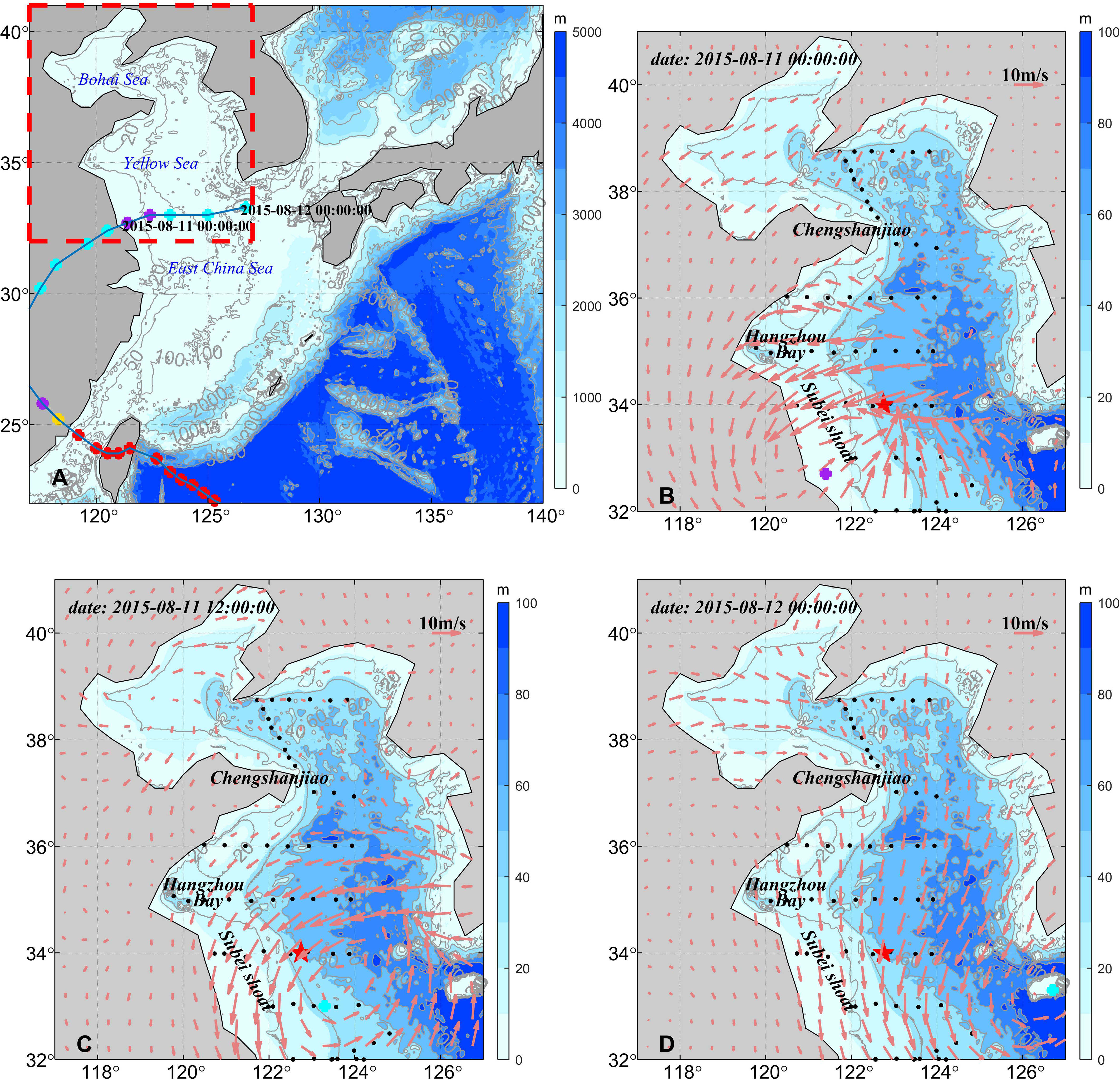
Figure 1 Model domain with topography (A) and the evolution of the wind field in the study area (B–D). The red dashed box represents the location of the Yellow Sea and Bohai Sea. The blue line represents the trajectory of the cyclone and the colored circle dots represent the intensity of the cyclone. The red, yellow, blue and purple circle dots represent typhoon, severe tropical storm, tropical storm and tropical depression, respectively. Colored shading and grey solid lines denote bathymetry. The black dots represent the locations of conductivity-temperature-depth profiler stations from the cruise surveys in August 2015. The red star represents the mooring station and arrows represent wind vectors.

In this study, two near-inertial energy peaks with inverse phases occurring in the mixed layer and at the base of the thermocline were identified by observations, rather than a homogeneous near-inertial energy below the thermocline. The dynamical processes of two near-inertial energy peaks are then investigated by improving the traditional two-layer model into a four-layer model. Furthermore, the influence of tides on near-inertial oscillations is studied using the high-resolution numerical model.

2 Data and methods

2.1 Observations

Measurements of temperature, salinity, and pressure were obtained using a conductivity–temperature–depth (CTD) system with Sea-Bird Electronics (SBE) 911plus implemented in a survey conducted in August 2015. The accuracies of the CTD sensors were 0.003 psu for salinity and 0.001°C for temperature. There were fifty-six CTD stations in the YS (Figure 1). The velocity profile was measured using a bottom-mounted 300-kHz Sentinel Acoustic Doppler Current Profiler (ADCP) located in the western YS (122.75°E, 34°N) from April to December, 2015. The depth of the mooring system was 74 m. The bin size of the ADCP observation was 2 m, with a sampling output interval of 30 minutes. In addition, SBE 37 CTD was mounted on the mooring system to simultaneously measure the bottom temperature, salinity, and pressure. Velocity data above a depth of 8m with poor quality were removed because of the effect of bubbles (Thorne and Hurther, 2014). The trajectory and intensity of the cyclone is downward from the Japan Meteorological Agency. (https://www.jma.go.jp/jma/index.html).

2.2 Regional ocean modeling system configurations

Regional Ocean Modeling System (ROMS) is a widely used free-surface, terrain-following, three-dimensional primitive equations ocean model that assumes hydrostatic and incompressible conditions (Shchepetkin and McWilliams, 2005). ROMS was used to study the response process of near-inertial flow in the YS during a cyclone transit and the model domain encompassed 22–42°N, 117.0–140.0°E (Figure 1A). The horizontal resolution was 1/18°× 1/18°. We adopt a 32-level stretched terrain-following vertical s-coordinates with control the surface and bottom parameters of θ_s=4.3, θ_b=0.4 to enhance the resolution near the surface and bottom (Shchepetkin and McWilliams, 2005). The minimum and the maximum water depths were set at 10 and 5, 000 m, respectively. The time steps for the inner and outer modes were 360 and 12 s, respectively. The outputs were stored every 1 h. Generic length scale (GLS) turbulence closure scheme was used to determine the vertical turbulent viscosity and diffusion coefficients for horizontal momentum equations and tracer equations. Background mixing coefficient for momentum is 1×10^-5 m²/s. Model was first integrated over 5 years for spin-up, from 1^st January, 2010 to 31^th December, 2014. Model continue to count to 31^th August, 2015.

The surface forcing fields include the wind field, atmospheric temperature, shortwave radiation, longwave radiation, atmospheric pressure, precipitation rate, and relative humidity derived from the European Centre for Medium-Range Weather Forecasts (ECMWF) through the Interim ECMWF re-analysis dataset with a temporal resolution of 1 h and a spatial resolution of 0.25° × 0.25° (http://apps.ecmwf.int/datasets). Based on these data, the net heat flux and freshwater fluxes in the model were calculated using the bulk formulation. The daily average sea surface temperature (SST) data were derived from the National Oceanic and Atmospheric Administration (NOAA)’s Optimum Interpolation Sea Surface Temperature v2.1, and Sea surface salinity was derived from the World Ocean Atlas 2013 (https://www.ncei.noaa.gov/). During model a spin-up period, SST and SSS are used to calibrate the model. Temperature, salinity, current velocity, and elevation of the open boundary and initial field were determined from the monthly average data set of the Simple Ocean Data Assimilation (SODA 3.4.1). The tidal constituents M2, S2, N2, K2, K1, O1, P1, and Q1 were introduced at the boundary. Their amplitudes and phases were interpolated from the 1/30°-resolution TPXO8-atlas solution of Oregon State University (OSU) Tidal Inversion Software (http://volkov.oce.orst.edu/tides/). Model bathymetry data were extracted from the General Bathymetric Chart of the Oceans (GEBCO) database with a resolution of 15 arc-second (http://www.gebco.net/). The topography was corrected using charts in shallow areas.

2.3 Methods

2.3.1 Normal mode decomposition

The dominant barotropic tides was extracted and removed by classic harmonics analysis program T_tide (Pawlowicz et al., 2002). The near-inertial velocity was obtained from residual flow of the mooring observations by band-pass filtering in the range of [0.95f 1.05f]. The vertical structure of the near-inertial velocity was determined by decomposing it into components of orthogonal vertical modes. The vertical structure of each mode is governed by the following equations (Gill, 1982; Thorpe and Jiang, 1998)

$\begin{array}{ll}\frac{{\partial }^2{\phi }_j\left(z\right)}{\partial z^2}+\frac{N^2\left(z\right)}{c_j}{\phi }_j\left(z\right)=0& (1)\end{array}$

$\begin{array}{ll}{\phi }_j\left(0\right)=0;{\phi }_j\left(-H\right)=0& (2)\end{array}$

Where c_j is the separation constant (eigenvalue), H is the total water depth, j is the mode number, and φ_j denotes the eigenfunction, which depends only on the buoyancy frequency (N) and the water depth. All equations are based on orthogonal Cartesian coordinates with x increasing eastward, y increasing northward, and z increasing upward and u, v, w are the x, y, z velocity components. The buoyancy frequency can be expressed as follows:

$\begin{array}{ll}N\left(z\right)={\left(-\frac{g}{\rho }\frac{\partial \rho }{\partial z}\right)}^{\frac{1}{2}}& (3)\end{array}$

Where g is the gravitational acceleration, ρ denotes density.

The vertical modes can be solved using Equation (1). The components of the near-inertial velocity (u_f) can be written as the sum of the modal contributions.

$\begin{array}{ll}{u}_f\left(z,t\right)={\sum }^{}{U}_j\left(t\right)\frac{\partial {\phi }_j\left(z,t\right)}{\partial z}& (4)\end{array}$

The modal velocity U_j was obtained by projecting the observed near-inertial velocity onto the vertical mode by least-squares regression at each time.

The high modes correspond to strong shear. The Richardson number (Ri) is used to describe the stability of the water column, which is related to stratification and shear.

$\begin{array}{ll}Ri=\frac{N^2}{S^2}=\frac{-\frac{g}{\rho }\frac{\partial \rho }{\partial z}}{{\left(\frac{\partial u}{\partial z}\right)}^2+{\left(\frac{\partial v}{\partial z}\right)}^2}& (5)\end{array}$

The Richardson number is normalised by the critical value of 0.25 (Song et al., 2013; Li et al., 2016) as follows:

$\begin{array}{ll}R{i}_n={\log }_{10}\left(Ri/0.25\right)& (6)\end{array}$

Therefore, when Ri_n (the normalized Richardson number) is lower than 0 (Ri_n < 0), the shear instability may develop, thereby inducing turbulent mixing.

2.3.2 Energy transfer and dissipation

Wind stress and friction act as sources and sinks of near-inertial kinetic energy (MacKinnon and Gregg, 2005). To examine the transition of near-inertial kinetic energy between the different modes, the work done by wind stress and friction in each mode is discussed. This method of energy calculation (Equations 7-16) is referenced from MacKinnon and Gregg (2005).

The depth-dependent wind stress T_s(z) is defined as:

$\begin{array}{ll}{T}_s=\{\begin{array}{c}\frac{{\tau }_s}{{\rho }_0{h}_m}, z\ge -h_m\\ 0, z\le -h_m \end{array}& (7)\end{array}$

Where h_m is the thickness of the surface mixed layer defined as the depth of the maximum buoyancy frequency square, ρ₀ denotes the sea water density approximated as a constant of 1025 kg·m^-3, and the wind stress τ_s is defined as:

$\begin{array}{ll}{\tau }_s={\rho }_a{C}_d\left|U_{10}\right|U_{10}& (8)\end{array}$

Where ρ_a denotes the air density and U₁₀ denotes the wind speed at 10 m. C_d is the wind stress drag coefficient, calculated using a method proposed by Large and Pond (1981).

The depth-dependent bottom stress T_b(z) is defined as follows:

$\begin{array}{ll}{T}_b\left(z\right)=\{\begin{array}{c}\frac{{\tau }_b}{{\rho }_0{h}_b}, z>-H+h_b\\ 0, z\le -H+h_b \end{array}& (9)\end{array}$

where h_b denotes the thickness of the bottom mixed layer and 30 m is used in this study. The reason for defining the bottom mixed layer thickness as 30 m is that the simulated near inertial velocities have a significant decay above 30 m depth of the sea bottom.

The bottom stress τ_b is calculated as follows:

$\begin{array}{ll}{\tau }_b=-{\rho }_0{C}_b\left|U_{bot}\right|U_{bot}& (10)\end{array}$

where U_bot is the deepest current vector and the bottom drag coefficient, and C_b, is the bottom stress drag coefficient, set to 0.0007 (Lu and Zhang, 2006; Song et al., 2021).

The baroclinic wind stress T_{s_bc}(z) and the baroclinic bottom stress T_{b_bc}(z) can be defined as follows:

$\begin{array}{ll}{T}_{s\_bc}=T_s\left(z\right)-\frac{1}{H}\underset{-H}{\overset{0}{\int }}{T}_s\left(z\right)dz& (11)\end{array}$

$\begin{array}{ll}{T}_{b\_bc}=T_b\left(z\right)-\frac{1}{H}\underset{-H}{\overset{0}{\int }}{T}_b\left(z\right)dz& (12)\end{array}$

The power input (${\left(\frac{dE}{dt}\right)}_{s,j}$) from each mode owing to the surface wind stress can be calculated as follows:

$\begin{array}{ll}{\left(\frac{dE}{dt}\right)}_{s,j}=\frac{1}{\eta +H}\underset{-H}{\overset{\eta }{\int }}\left[U_j\left(t\right)·T_{s\_bc}\left(z,t\right)\right]\frac{\partial {\phi }_j\left(z\right)}{\partial z}dz& (13)\end{array}$

Where E denotes the accumulated energy and η denotes the sea surface elevation.

The power lost (${\left(\frac{dE}{dt}\right)}_{b,j}$) from each mode owing to the bottom drag can be calculated as follows:

$\begin{array}{ll}{\left(\frac{dE}{dt}\right)}_{b,j}=\frac{1}{\eta +H}\underset{-H}{\overset{\eta }{\int }}\left[U_j\left(t\right)·T_{b\_bc}\left(z,t\right)\right]\frac{\partial {\phi }_j\left(z\right)}{\partial z}dz& (14)\end{array}$

2.4 Model validations

2.4.1 Temperature and salinity validation

To examine whether the model results capture the hydrographic features of the YS, the observed bottom temperature is first compared with model simulated bottom temperature averaged over the month of August (Figures 2A, B). The YSCWM occupied the central part of the Yellow Sea, with a 10°C envelope. The range and temperature of the YSCWM in the model results are slightly broader and lower than those in the observations which may be related to the choice of turbulence closure scheme (Bi et al., 2021). Figures 2C, D show the comparison of observed and simulated monthly mean temperatures along 35°N. In the coastal region, the temperature at the full depth was almost uniform owing to tidal-induced mixing and surface waves (Qiao et al., 2006). A temperature front that separated the cold water on the offshore side from the warm water on the other side existed at the edge of YSCWM. In the central Yellow Sea, the stratification is significantly stronger than that in coastal waters, due to the presence of YSCWM. The root-mean-square error (RMSE) between the temperature observed by SEB 37 and the model bottom temperature at the mooring site is 0.33°C in August. However, some defects persist in the model results. It should be noted that the simulated temperature is much stronger than the observations in the Subei shoal, which may be a result of the stronger heat flux input inshore. The thickness of the upper mixed layer is underestimated by the simulations, probably due to the absence of wave mixing effects (Qiao et al., 2006) and turbulence closure scheme (Bi et al., 2021).

FIGURE 2

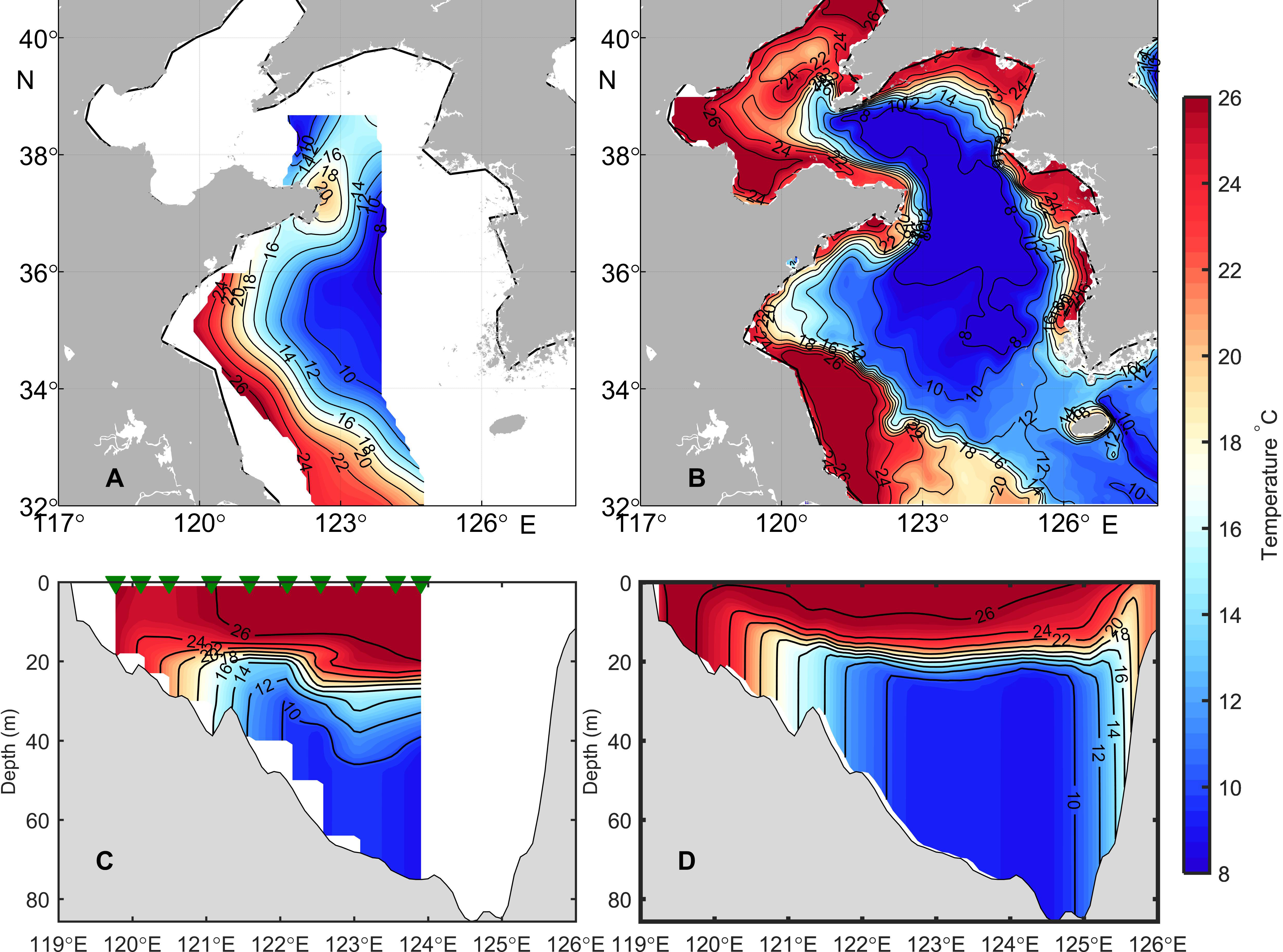
Figure 2 Bottom temperature distribution of in situ observations (A) and monthly mean model results (B) in August 2015. Temperature distributions of in situ observations (C) and monthly mean model results (D) at the 35°N section in August 2015. The triangles in (C) denote the conductivity-temperature-depth stations.

The observed bottom salinity is compared with model simulated bottom salinity averaged over the month of August (Figures 3A, B). The range and salinity of the YSCWM with a 32.5 psu envelope in the model results are slightly narrower and lower than those in the observations. The distribution of salinity section has the same structure as the temperature distribution (Figures 3C, D). A salinity front separated the stratified high salinity water on the offshore side from mixed low salinity water on the other side existed at the edge of YSCWM. The RMSE between the bottom salinity from the SBE 37 observations and the model is 0.4 psu in August.

FIGURE 3

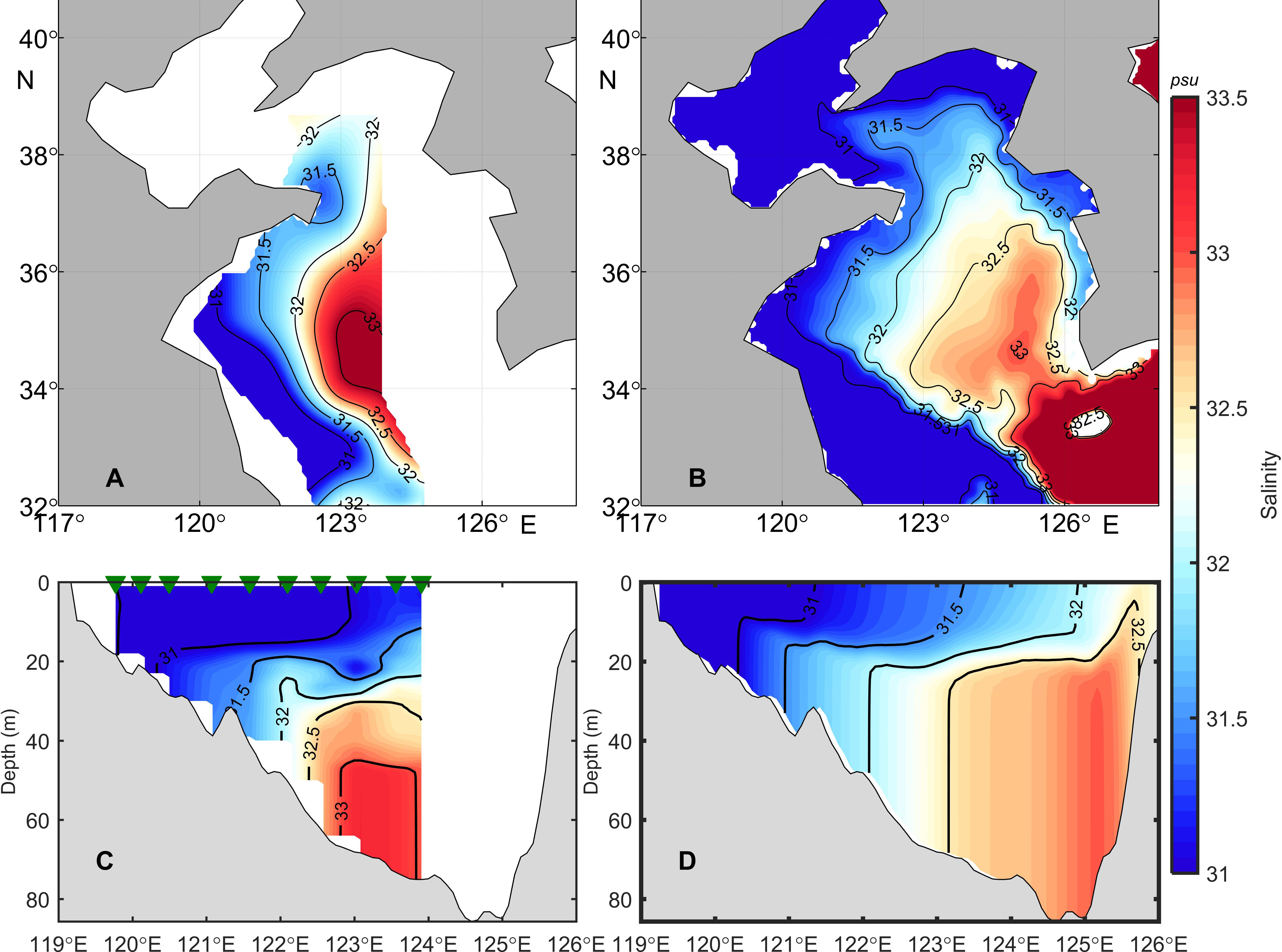
Figure 3 Bottom salinity distribution of in situ observations (A) and monthly mean model results (B) in August 2015. Salinity distributions of in situ observations (C) and monthly mean model results (D) at the 35°N section in August 2015.

In contrast to the vertical variation in temperature, the vertical variation in salinity is small, with a maximum difference in salinity of 2 psu between the surface and bottom layers. Temperature is the most distinctive feature of YSCWM and has the greatest influence on stratification. So, the article focuses mainly on temperature. An error of ~0.3°C in the bottom layer temperature has little effect on the stratification. The focus of our attention is on the dynamical processes under strong stratification. It can be assumed that the ROMS generally captures the hydrographic characteristics of the YS.

2.4.2 Tide validation

The YS is a strongly tidally-driven shelf sea. Strong tides play an important role in driving the turbulence and mixing (Qiao et al., 2006; Liu et al., 2009; Meng et al., 2020). The verification of tides is important for validating model results. Considering that the M₂ constituent as the most predominant tidal component, the modelled co-tidal charts of the M₂ constituent (Figure 4A) is generally consistent with previous studies (Wan et al., 1998; Zhang et al., 2005). As shown in Figures 4B, C, the amplitude and phase of the modelled M2 tide are compared with the 75 tidal gauges along the coastline. The observed data were derived from 75 tide gauges (the black spots in Figure 4) provided by Wan et al. (1998). The correlation coefficients between the observed and modelled tidal amplitudes and phases are 0.96 and 0.98 (at the 95% confidence level), respectively, with RMSEs of 15.7 cm and 36.0°, respectively. Two amphidromic points in the YS are located offshore of Chengshanjiao and Haizhou Bay.

FIGURE 4

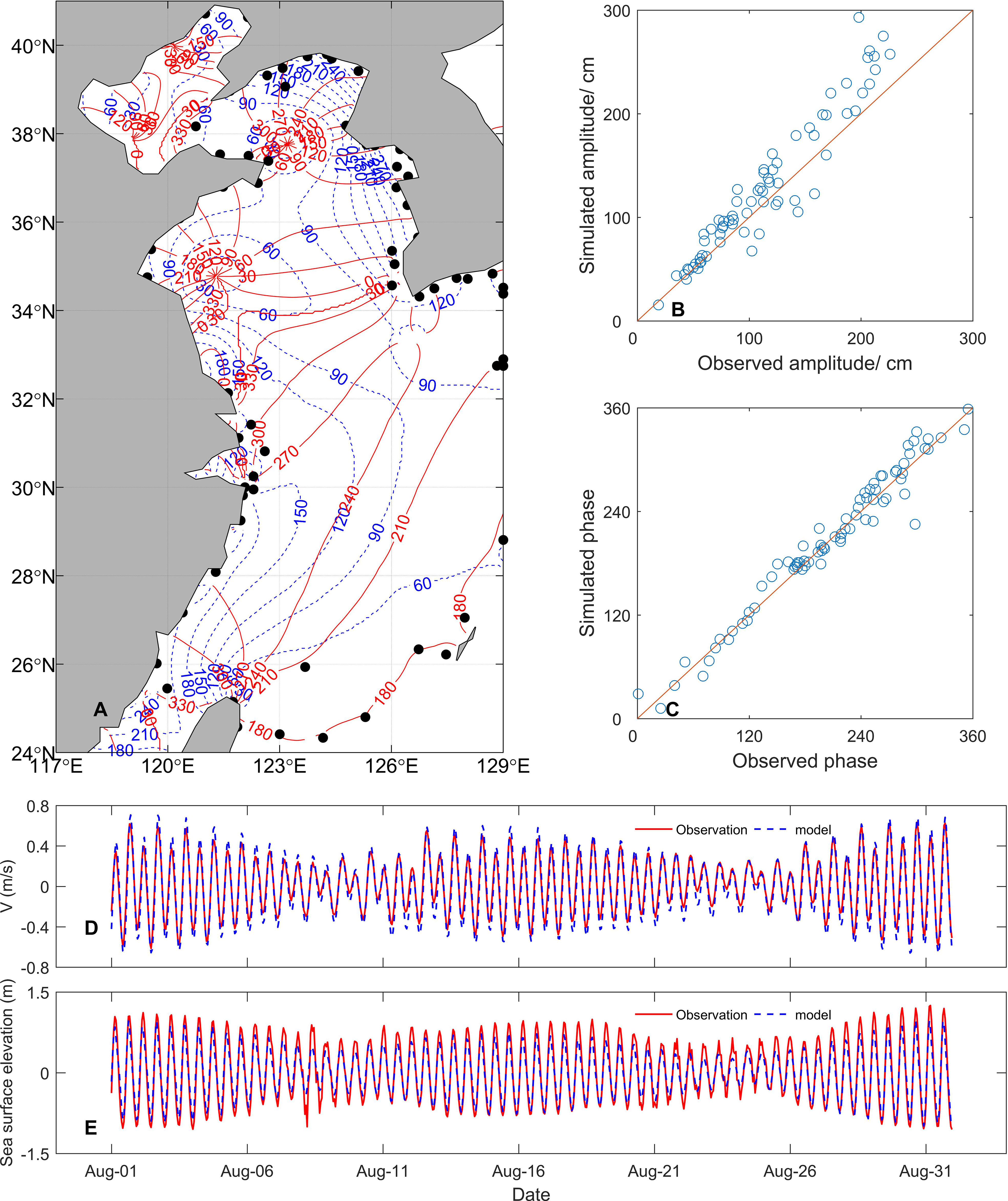
Figure 4 Modelled cotidal charts (A) of M₂. The blue dashed lines and red solid lines denote the amplitude (cm) and phase lags (degrees), respectively. The black dots denote locations of 75 tide gauges (A). Comparison between the modelled and observed amplitudes (B) and phase lags (C) at 75 tidal gauges. Comparison between the modelled and observed depth-mean meridional velocity (D) and sea surface elevation (E) at the mooring site. The blue and red lines in the (D) and (E) represent model results and observations, respectively.

The simulated barotropic tide flow and sea surface elevation were compared with observations. The correlation coefficient between the observed and modelled meridional velocity and sea surface elevation are 0.97 and 0.96 (at the 95% confidence level), respectively, with the RMSE of 0.10m/s and 0.17m, respectively. The bias in the barotropic tide is mainly related to the topography and the bottom friction coefficient.

2.4.3 Near-inertial oscillation verification

Typhoon Soudelor was generated in the Central Pacific on 29^th July 2015 and moved northwestwards. Soudelor made landfall in southeastern mainland China, rapidly decreasing in intensity and moving northeastward as shown in Figure 1. As it entered the Yellow Sea at 00:00:00 on 11^th August, it had declined into a tropical cyclone with a maximum wind speed of 30 m/s. Cyclone completely removed on 12^th August. Although the cyclone lasted only two days, a near-inertial oscillation event sustained over 10 days was observed and modelled between 11^th and 20^th August 2015 (Figure 5). The simulated near-inertial flow resolves the basic characteristics of the observations, including the inverse phase relationship and the two velocity peaks (Figure 5). The magnitude and thickness of the simulated near-inertial flow peak in the upper layer are higher and thinner than observed, respectively, probably because the depth of the simulated mixed layer is shallow relative to the true value. Based on the slab model (Alford, 2001), at shallower mixed layer depths, the near-inertial velocity of the wind input to the mixed layer is greater. Due to the shallowing of the mixed layer and the expansion of the YSCWM, the position of the maximum stratification (blue line in Figure 5A) is lifted, resulting in an upward shift in the position of the peak inertial velocity in the lower layer. However, the magnitude and thickness of the simulated lower velocity peak is generally consistent with observations. This study focuses on the dynamical processes of the two velocity peak structures and the position bias of the peak inertial velocity does not affect the conclusions.

FIGURE 5

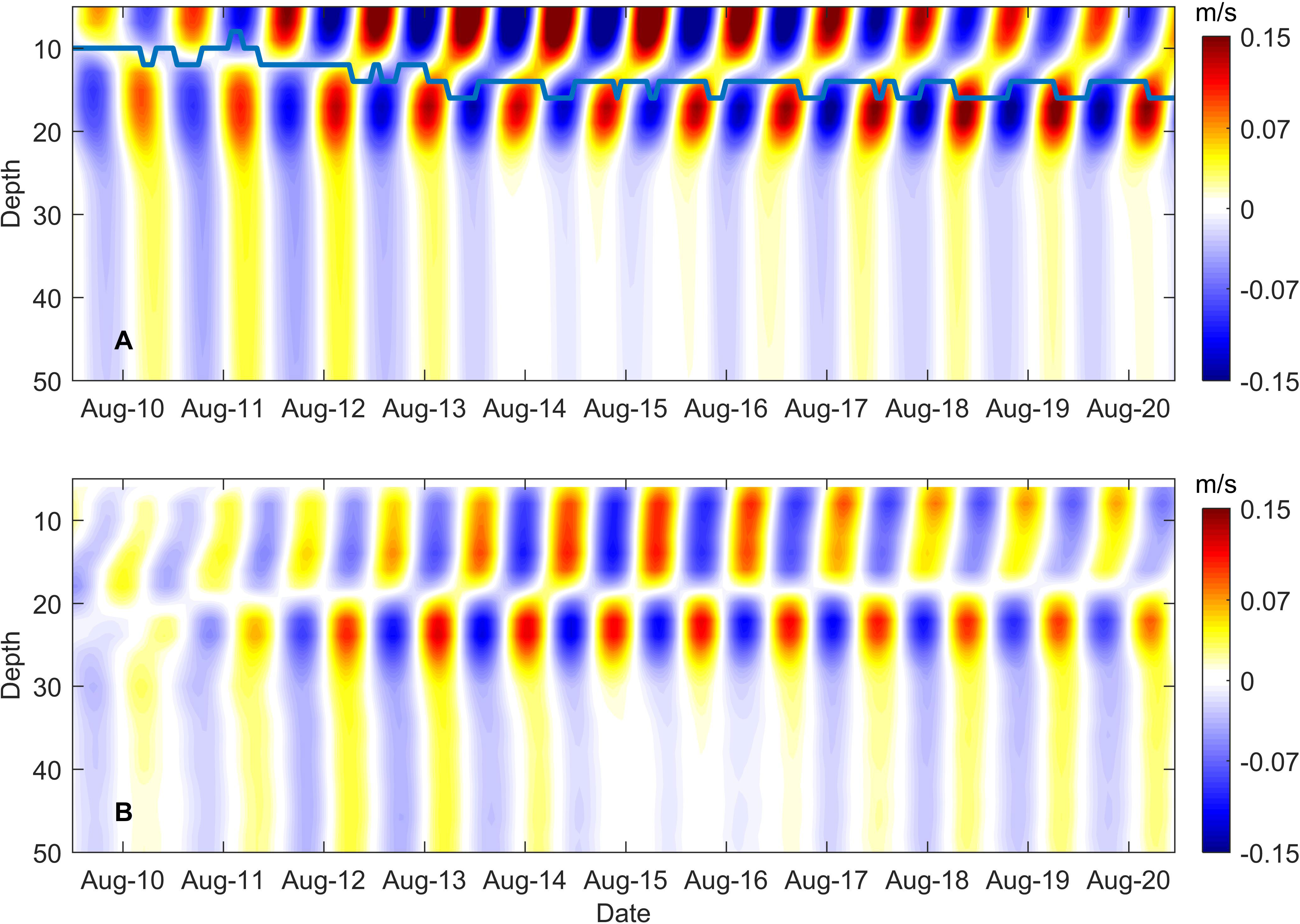
Figure 5 Modelled (A) and observed (B) near-inertial velocities (m/s) at the mooring site. The blue line in the (A) denotes the depth of the maximum stratification of the simulation.

3 Results

3.1 Two velocity peaks above and below the maximum stratification

Two noticeable near-inertial velocity peaks are found in the upper mixed layer and below the maximum stratification, with a velocity of up to 0.15 m/s (Figures 5, 6A). From the mixed layer to the thermocline, the near-inertial velocity decreases rapidly. The vertical structure of the near-inertial flow was dominated by a 180° phase difference with one zero-crossing at the depth of the maximum stratification (the blue line in Figure 5A). A near-inertial peak occurs from the depth of the maximum stratification to a depth of 20 m. In the bottom boundary layer, the near-inertial velocity was very weak at approximately 0.03 m/s.

FIGURE 6

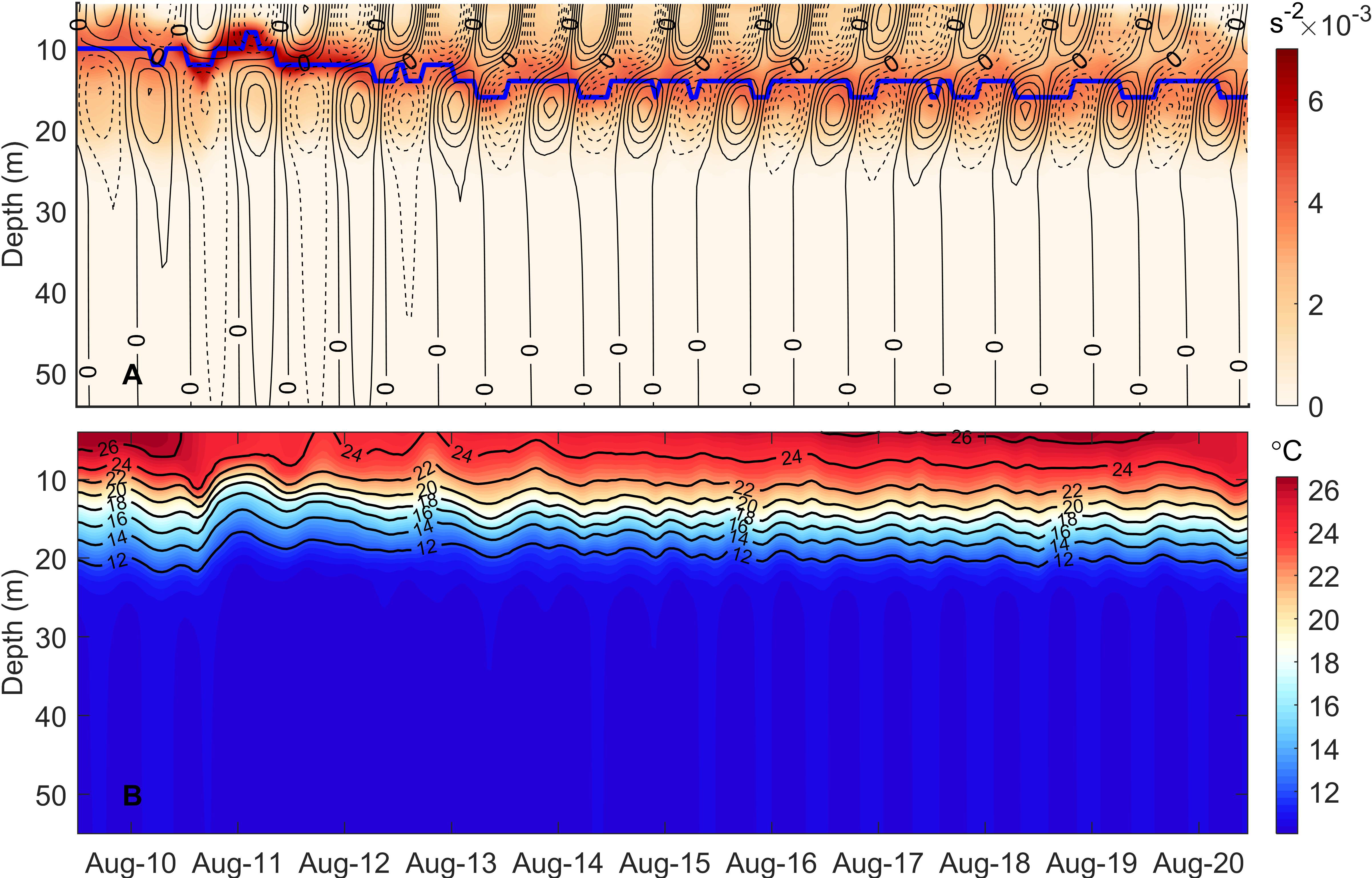
Figure 6 (A) N² (orange shading) and alongshelf near-inertial velocity (black contour lines) at the mooring site from ROMS. The black solid and dashed lines represent positive and negative values, respectively. Contour interval for velocity is 0.03m/s. The blue line represents the depth of the maximum stratification. (B) The modelled temperature (°C) at the mooring site from ROMS.

The vertical structure of the antiphase of near-inertial flow is closely dependent on the stratification and can be explained by the traditional two-layer model (Millot and Crépon, 1981; Kelly, 2019). The wind-generated near-inertial flow was confined within the mixed layer and could not pass through the thermocline, due to the strong stratification which suppresses the downward transfer of near-inertial energy (Davies and Xing, 2005; Yang et al., 2015). Below the thermocline, however, owing to the presence of the coast, the pressure gradient force formed by the convergence and divergence of seawater induces a near-inertial flow with an opposite phase to satisfy the cross-shelf flux conservation (Millot and Crépon, 1981; Davies and Xing, 2005; Shearman, 2005). However, the phenomenon of strong near-inertial velocity peaks at the base of the thermocline, which should be homogeneous below the thermocline according to the two-layer model, has not been explained.

While triggering near-inertial oscillations, the cyclone also has an influence on the stratification of the YS. Firstly, the model shows ~2°C cooling of the SST at the observation site associated with the arrival of the cyclone (Figure 6B). ln contrast to surface heat flux that dominates over the open ocean, the entrainment term is the dominant process for significant SST cooling in the YS (Moon and Kwon, 2012; Lee et al., 2016; Yang et al., 2019). Then, the deepening of the mixed layer caused by wind stirring results in the compression of the thermocline which then intensifies and deepens the maximum stratification strength and depth, respectively. Prior to the arrival of the cyclone, N², which represents the strength of the maximum stratification, was ~4×10^-3 s^-2 located at 10m, while after the cyclone the N² strengthened to ~6×10^-3 s^-2 and deepened to 13m. Note that the maximum depth of stratification become shallower first, which can be related to cyclone-induced upwelling (Jacob et al., 2000) which can be confirmed by the lifting of temperature contours on the 11^th of August (Figure 6B). The maximum depth of stratification is deepening after the cyclone.

3.2 Vertical structure and shear of near-inertial flows

The first baroclinic mode can explain the flow structure of the upper and lower opposite phase, but the theoretical maximum flow velocities in the first baroclinic mode occurring at the surface and the bottom layers are inconsistent with observations (i.e. strong near-inertial flow occurs below the thermocline in the observations and model). To examine the vertical structure of the near-inertial velocity, the modelled near-inertial velocity was projected onto the first five baroclinic modes using a least-squares regression at each time according to Equations (1) - (4).

The vertical structure of the first three modes and the percentage of each mode’s energy to the total energy were calculated and shown in Figure 7. It was found that the near-inertial energy was dominated by the first model energy, accounting for 60% of the total energy, and was mainly distributed in the mixed layer and below a depth of 20m. However, at depths below the maximum stratification from 10 to 20m, the second modal energy dominated rather than the first mode; and the first and the second mode velocities were in phase, causing the peak of near-inertial energy at this depth (purple and red lines in Figure 7A). The near-inertial velocity peak is not revealed by the first-mode structure solely, but by the increase in higher-order mode energy due to other physical processes. The higher modal energy was associated with strong friction under the influence of the tides and was significantly reduced when the tidal currents disappeared, which will be clarified in the following discussion.

FIGURE 7

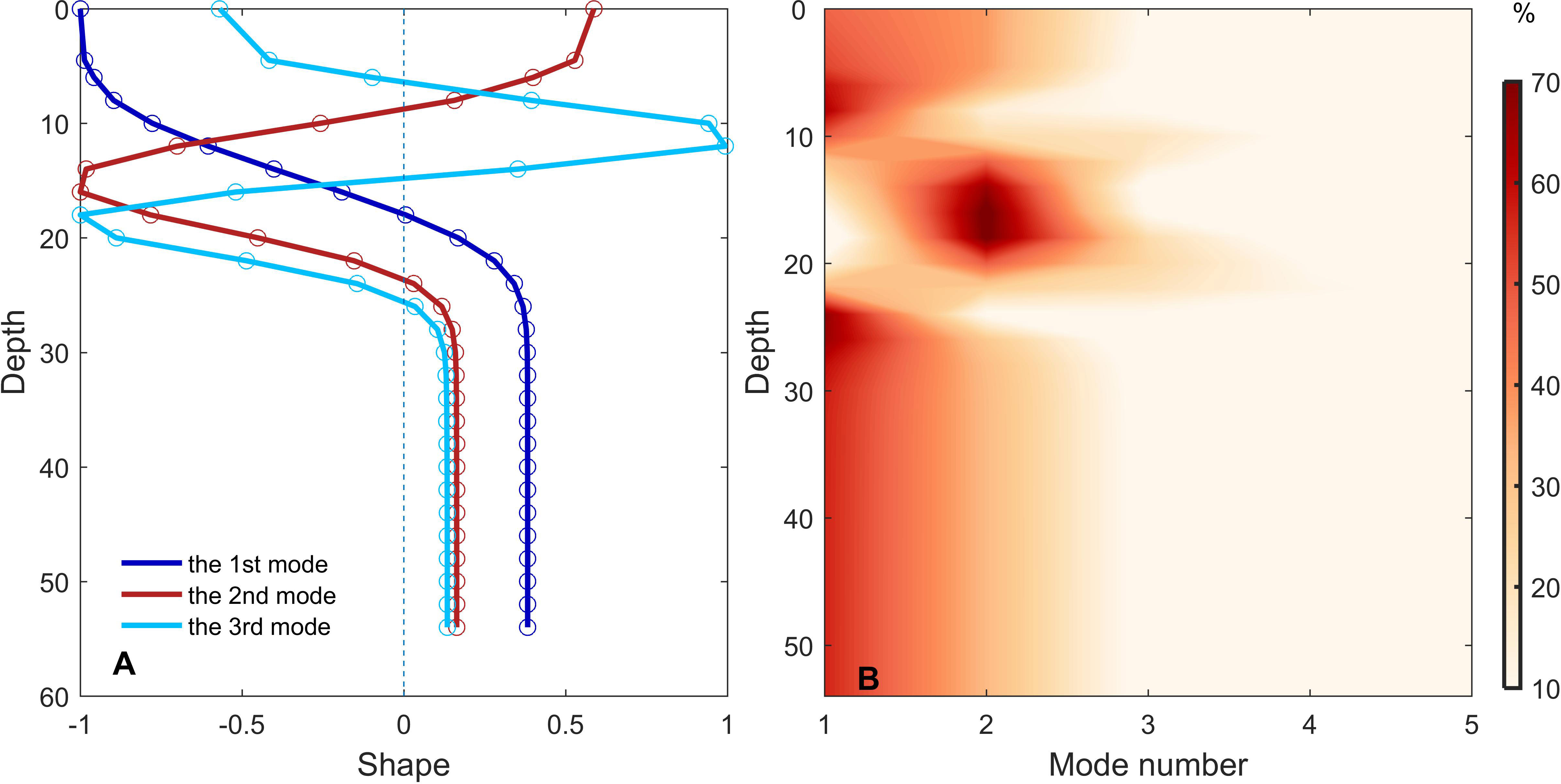
Figure 7 (A) Vertical structures of the first three modes of the near-inertial velocity at the mooring site. (B) The percentage of the energy in each mode to the total energy at different depths.

To elucidate the sources and sinks of energy in each mode, the energy gain and loss of each mode from the wind and bottom friction are calculated using Equations (12) –(13). The energy of the modes 1 and 2 gained or lost from bottom friction is shown in Figure 8A. Although the cumulative work done by the bottom friction in mode 2 was weak, the positive work suggested that the bottom friction was a source of energy in mode 2 (blue line in Figure 8A). However, the negative cumulative work done by the bottom friction in mode 1 indicated that the bottom friction was a sink of energy for mode 1 (red line in Figure 8A). The energy of mode 1 and 2 gained or lost from wind is shown in Figure 8B. The work done by wind in mode 1 increased rapidly and positively on 11^th August indicating that wind was a source of energy for mode 1. The work done by wind in mode 2 was minor but positive, indicating that the wind also input a slight amount of energy for mode 2.

FIGURE 8

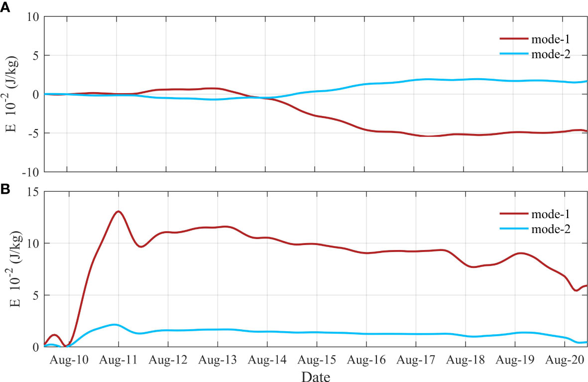
Figure 8 Energy (J/kg) gain and loss of each mode from (A) the bottom friction and (B) wind at the mooring site. The red and blue lines represent the first and second mode energy, respectively.

The near-inertial velocity with opposite phase led to the maximum shear value at the thermocline (at depths of 10m-20m), while the higher modal energy contributed to the sub-peak in shear below the thermocline (Figure 9A). The normalised Richardson number (Ri_n) is used to justify the shear instability according to Equation (6). Although the shear was the strongest within the thermocline, the Ri_n greater than zero indicated the development of the shear instability inhibited by strong stratification (Figure 9B). Below the thermocline, the Ri_n decreased and was even less than zero relative to that within the thermocline, suggesting the occurrences of the shear instability due to the stratification below the thermocline being at its weakest. On August 11^th, Ri_n was less than 0 at a depth of 20-30m, which indicates the occurrence of shear instability (Figure 9B). This shear instability may cause the underlying cold water to mix into the thermocline.

FIGURE 9

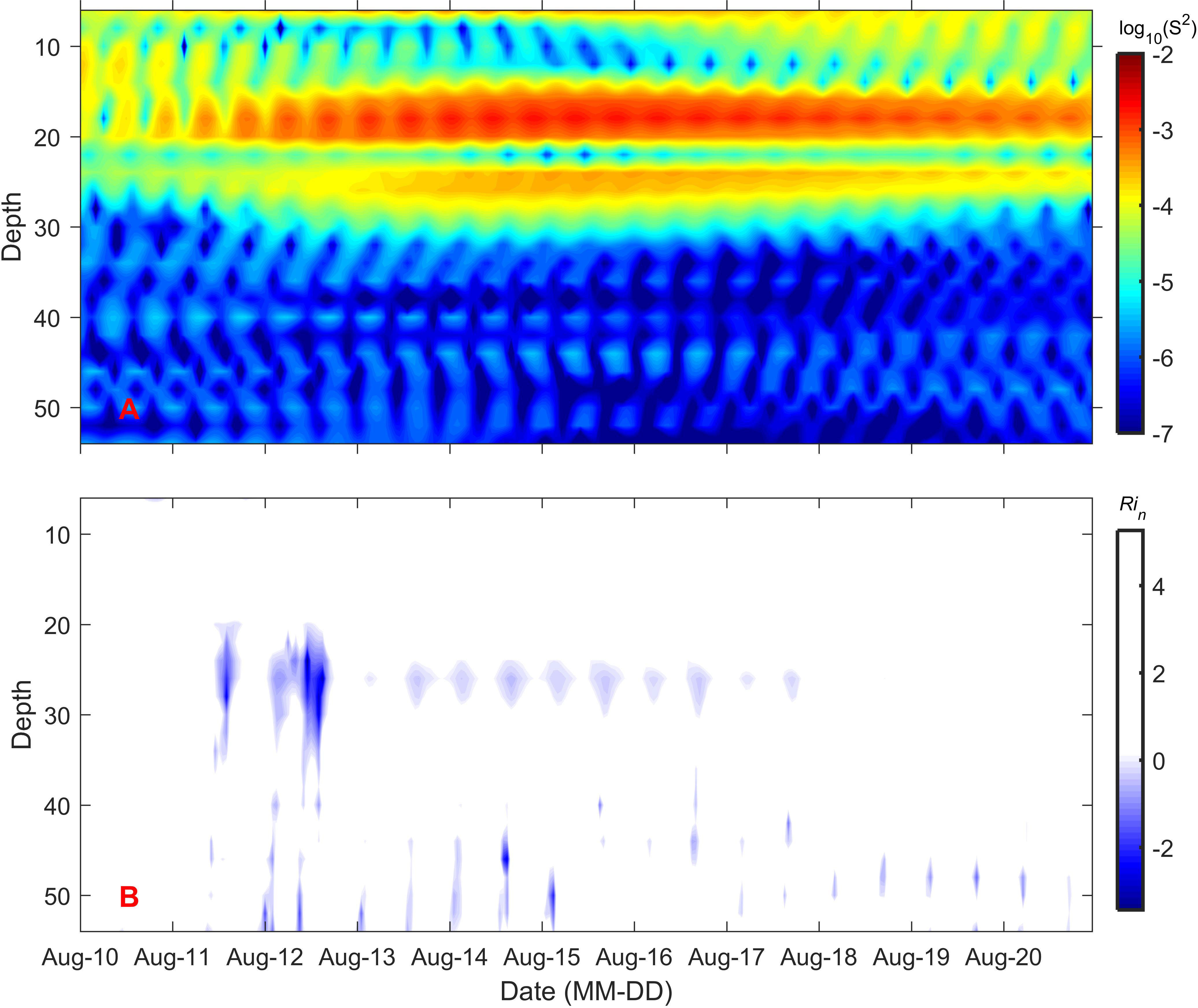
Figure 9 (A) Shear (log₁₀S²) of the near-inertial flow and (B) the normalised Richardson number at the mooring site.

3.3 Relationship between the section distribution of near-inertial kinetic energy and wind stress and stratification

The horizontal distribution of near-inertial velocity is shown in Figure 10A. In the coastal region, tidal-induced mixing led to the disappearance of the stratification, and the near-inertial oscillation was in phase throughout the water column. In shelf seas, with the increase in the depth and the enhancement of the stratification, the near-inertial velocity is in antiphase above and below the thermocline, with one zero-crossing at the depth of the maximum stratification (bold black line in Figures 10A, B).

FIGURE 10

Figure 10 (A) Horizontal distribution of near-inertial velocity (m/s) at 12:00:00 on 11th August 2015 at 34°N from ROMS. (B) is the same as (A) but for averaged NIKE (J). (C) Zonal distribution of wind energy input (KJ·m^-2). (D) Zonal-time plot of phase (theta =actan ($\frac{v_f}{u_f}$)). The thick and thin black line in (A, B) represent the maximum stratification depth and water depth, respectively.

In the coastal region (121°-122.2°E), despite the strong influence of wind stress, the near-inertial flow was very small, at 0.02 m/s. This value can be attributed to the friction caused by the shallow water depth in this region (Figures 10A–C),which causes the wind energy input to be dissipated in the form of seiches on a much smaller scale (Anderson et al., 1983; Sobarzo et al., 2007; Chen et al., 2017). In the mixed layer of the shelf region from 122.5° to 123°E, the near-inertial kinetic energy (NIKE) was enhanced with the increasing of the wind work, indicating that the NIKE was related to wind work. Below the thermocline of the shelf region from 122.2° to 123°E, the location of the maximum NIKE was at the shelf break (122.4°E). To satisfy cross-shelf flux conservation, the near-inertial velocity below the thermocline is related to that in the mixed layer and the water depth below the thermocline. The NIKE below the thermocline of the region from 122°E to the shelf break and from the shelf break to the 123°E was weaker than that at the shelf break because of the weak NIKE in the mixed layer and the deep water depth below the thermocline,respectively. As shown in Figure 10B, the maximum NIKE in the mixed layer occurred at 123°E, where wind energy input was greatest, and the maximum NIKE energy below the thermocline occurred at the shelf break.

The clockwise rotation of the near-inertial velocity indicated a decreasing phase with time and downward transmission of near-inertial energy. Owing to the rapid propagation of the barotropic wave, the phase was almost uniform in the region of 122.2°E to 124°E, with the offshore phase slightly lagging behind the nearshore phase (Figure 10D).

4 Discussion

4.1 Roles of tides in the near-inertial flow

The YS is a strongly tidally-driven shallow shelf sea, dominated by the M₂, with a maximum value of up to 0.5 m/s. Tides have a significant influence on the hydrological environment and circulation structure of the YS (Xia et al., 2019; Meng et al., 2020); therefore, an understanding of the effect of tides on the near-inertial flow is crucial.

To investigate the influence of tides on the near-inertial velocity, we simulated the near-inertial velocity with and without the tides (Figures 5A, 11). The most striking phenomenon is the variation in the vertical structure of the near-inertial current. Under the influence of the tides, the strong near-inertial velocity below the maximum stratification were mainly concentrated between 10-20 m. However, in the absence of tides, the strong near-inertial response extended to 40 m with a significant weakening within the bottom 10 m. The results suggest that the near-inertial energy was dominated by the second modal energy between 10-20 m below the thermocline with the influence of tides. However, the near-inertial energy was dominated by the first modal energy without the influence of tides according to the model analysis. As analysed in result 3.2, an increasing of tides increases bottom friction, which is a source of higher modal energy and a sink for first modal energy. The absence of tidal currents decreases bottom friction resulting in a decrease in higher modal energy and an increase in first modal energy.

FIGURE 11

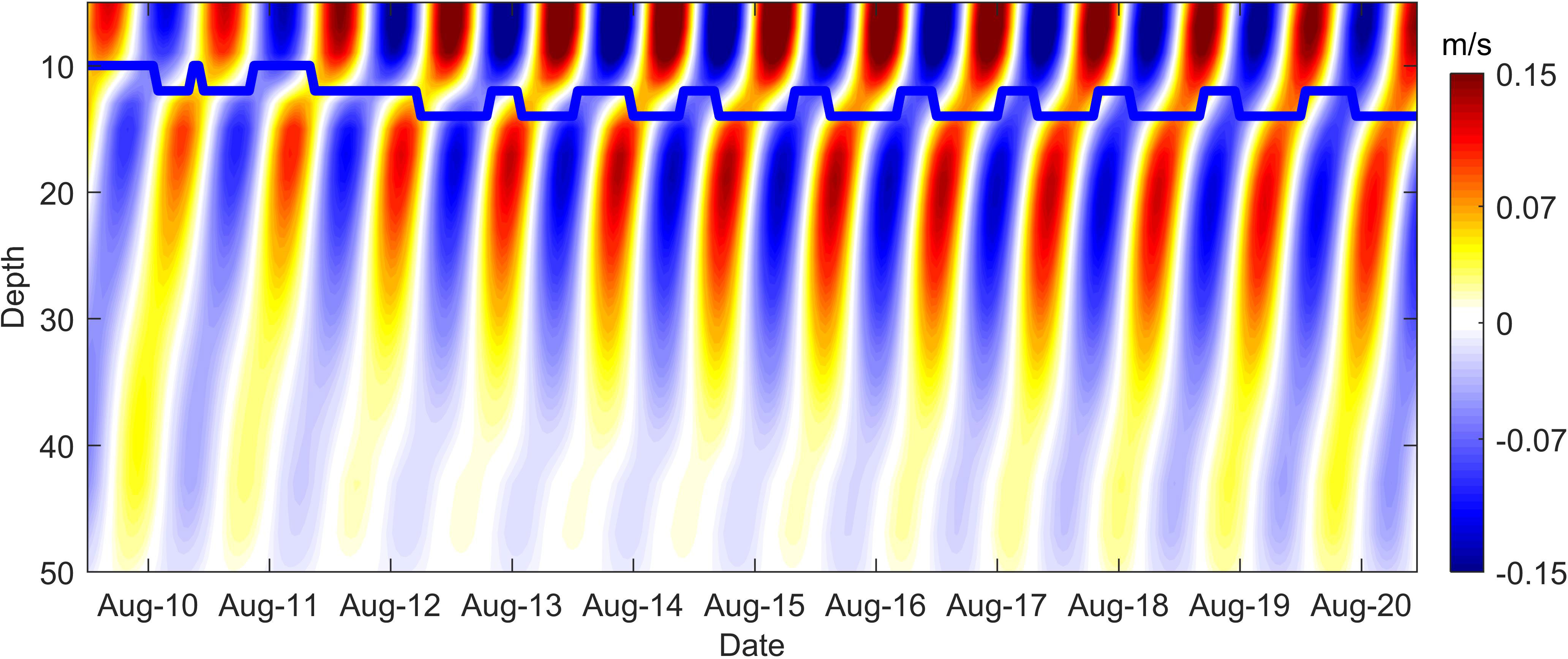
Figure 11 The simulated near-inertial velocity (m/s) at the mooring site in the absence of tide. The blue line denotes the depth of the maximum stratification of the simulation.

To investigate how tides affect the near-inertial flow, eddy viscosities with and without tides were simulated. Within the mixed layer, the near-inertial energy input from wind energy became homogeneous under the influence of the eddy viscosity during the period of wind energy input from 10^th to 12^th August. Below the thermocline, eddy viscosity was mainly related to the influence of tides. As shown in Figures 6A, 11, during the presence of tides, the eddy viscosity is uniform up to 20 m depth, where it corresponds to a weak near-inertial velocity. Strong peak near-inertial velocities correspond to weak eddy viscosity at 10-20 m depth. In the absence of tides, eddy viscosity in the lower layer was mainly confined within 10 m of the bottom boundary, resulting in a significant reduction in near-inertial flow (Figures 11, 12B). From the depth of the maximum stratification to 40 m, the eddy viscosity is low corresponding to strong near-inertial flow velocities. In brief, mixing leads to rapid diffusion of near-inertial energy above the thermocline, which is generated by wind stress. Below the thermocline, the near-inertial energy is suppressed by the eddy viscosity. The effect of eddy viscosity is pronounced in the existence of tides.

FIGURE 12

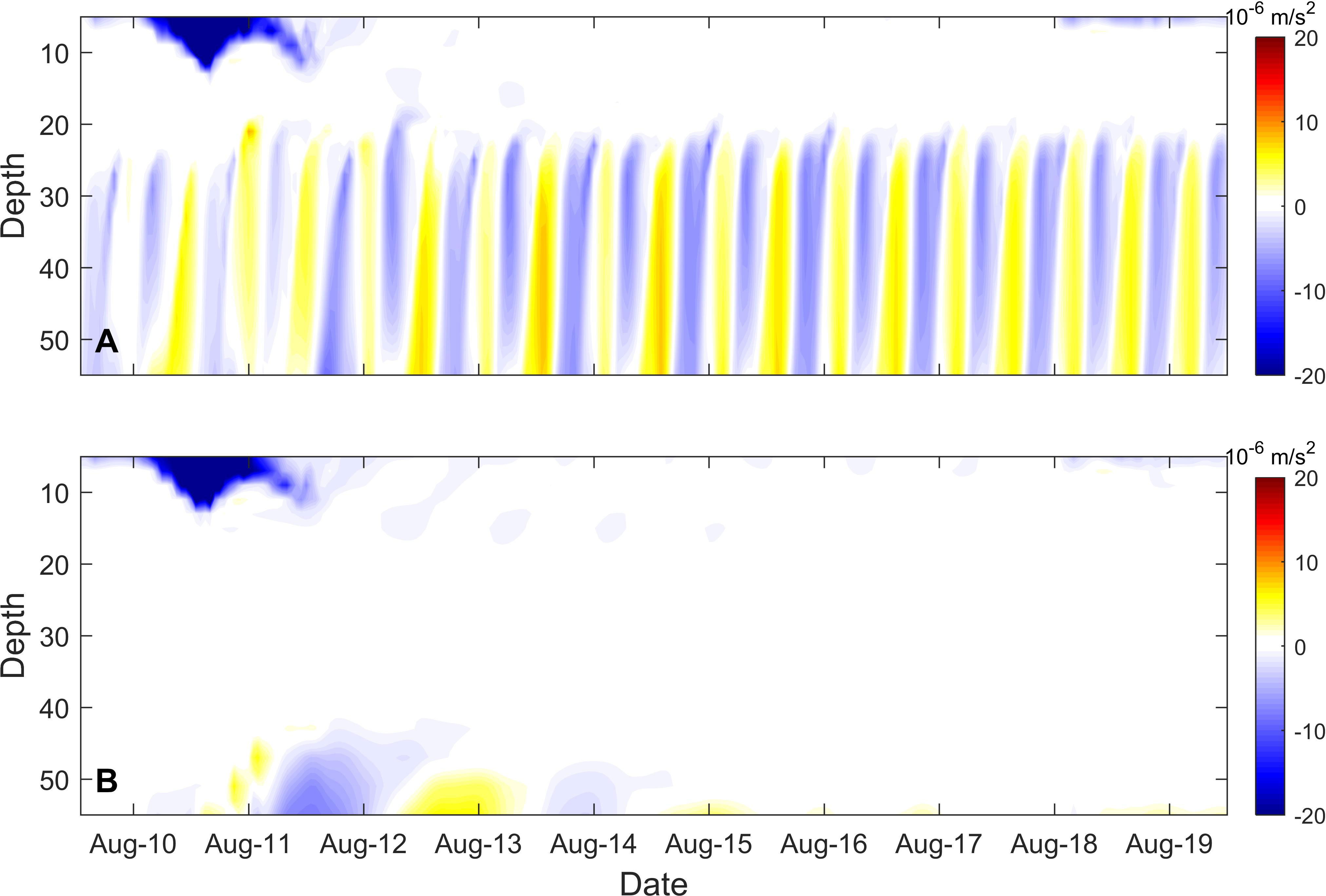
Figure 12 Eddy viscosity (m/s²) at the mooring site (A) with and (B) without tides.

In different shelf seas, the vertical structure of the near-inertial current may differ due to different tidally induced eddy viscosities. In strongly tidally-driven shelf seas, a narrower depth near-inertia peak occurs due to the deep influence of eddy viscosity (Figures 5A, 12A). When the tide is not strong or disappears, the eddy viscosity affects a limited range of depths, and a near-inertia peak with a wider depth occurs (Figures 11, 12B). Further observations are needed to confirm this view.

4.2 Response of near-inertial flow to wind

The traditional two-layer model assumes that the time-varying wind field induces a near-inertial flow at the surface layer and the energy input from the wind cannot break through the thermocline to propagate downward. During the forcing phase, the wind causes the seawater to accumulate along the coast. The accumulated seawater is released during the geostrophic adjustment process and barotropic waves are generated at the coast and propagate offshore, which suppress the near-inertial flow response in the upper layer but generate the near-inertial flow in the lower layer (Millot and Crépon, 1981; Shearman, 2005).

Previously, the non-linear and eddy viscosity were not considered in the control equations of the two-layer model. Although, the two-layer model can appropriately account for the relationship between the inertial velocity inversions above and below the thermocline, the dynamical process of the two velocity peaks in the mixed layer and below the thermocline remains unclear. Given that the pressure gradient forces are uniform throughout the water column, it is unclear why the inertial velocity within the thermocline and bottom boundary layer is small compared with the inertial velocity peaks in the mixed layer and below the thermocline. In the YS, the ocean should be divided into four layers according to the characterstics of near-inertial velocity: the mixed layer with velocity peaks at depths above 10 m, the thermocline, the lower mixed layer with velocity peaks at depths of 10-20 m, and the bottom boundary layer with rapidly decreasing velocity (Figures 5, 11). To investigate the response of the ocean to time-varying wind fields, the original N-S equation is given as:

$\begin{array}{ll}\frac{\partial u}{\partial t}+u\frac{\partial u}{\partial x}+v\frac{\partial u}{\partial y}+w\frac{\partial u}{\partial z}-fv=-\frac{1}{\rho }\frac{\partial p}{\partial x}-\frac{1}{\partial z}\left(-K_M\frac{\partial u}{\partial z}\right)-\frac{1}{\partial z}\left(ɤ\frac{\partial u}{\partial z}\right)& (15)\end{array}$

In Equation (15), ɤ and K_M denote molecular viscosity coefficient and eddy viscosity coefficien, respectively. The terms of acceleration $\frac{\partial u}{\partial t}$, horizontal advection $u\frac{\partial u}{\partial x}$ and $v\frac{\partial u}{\partial y}$, convection $w\frac{\partial u}{\partial z}$, Coriolis force -fv, pressure gradient force $-\frac{1}{\rho }\frac{\partial p}{\partial x}$, eddy viscosity $-\frac{1}{\partial z}\left(-K_M\frac{\partial u}{\partial z}\right)$, and molecular viscosity term $\frac{1}{\partial z} \left(ɤ\frac{\partial u}{\partial z}\right)$ are shown in order from left to right in Equation (15). The minor terms of the horizontal advection are ignored relative to the convection term. In addition, the molecular viscosity term can also be ignored relative to the eddy viscosity term.

Therefore, Equation (15) can be rewritten as follows:

$\begin{array}{ll}\frac{\partial u}{\partial t}+w\frac{\partial u}{\partial z}-fv=-\frac{1}{\rho }\frac{\partial p}{\partial x}-\frac{1}{\partial z}\left(-K_M\frac{\partial u}{\partial z}\right)& (16)\end{array}$

In the absence of tide, the diagnostic analysis of each layer is illustrated in Figure 13. The response of the ocean to time-varying wind fields first appeared in the mixed layer (Figure 13A). During the wind-forced period from 12:00 on the 10^th to 00:00 on the 11^th August, the velocity increased with the increased in wind stress, and the acceleration term and the Coriolis force combined to balance the wind stress. During the wind-forced period, wind-driven currents caused seawater to accumulate on the shore, creating enhanced offshore pressure gradient forces at all depths. As the wind stress decreased on 11^th August, seawater at the shore was released and propagated offshore, causing a decrease in pressure gradient force (blue line in Figure 14). A barotropic wave was first generated at the coast at 00:00 on 11^th August and propagated offshore. A comparsion of the variation in pressure gradient force with time at different positions reflects the gradual decrease in amplitude during the wave propagation (Figure 14). As the barotropic wave propagated to 124°E, the pressure gradient force decreased significantly so that near-inertial kinetic energy below the thermocline became almost zero (Figure 10B). From 00:00 on 11^th to 00:00 on 12^th August, the magnitude of the wind stress gradually decreased, and the pressure gradient force gradually increased. At this stage, the terms of acceleration, Coriolis force, pressure gradient force, and eddy viscosity were balanced. When the wind stress disappeared completely at 20:00 on 11^th August, the pressure gradient force was at its maximum, and the Coriolis force was smaller than that when the wind stress was at its maximum. In other words, the arrival of a barotropic wave will weaken the near-inertial flow of the mixed layer (Millot and Crépon, 1981). Finally, the seawater motions were mainly balanced by the terms of acceleration, Coriolis force, and the pressure gradient force. Therefore, the motions appeared in the form of a near-inertial frequency. When the pressure gradient force disappeared from 00:00 on 15^th August, the motions became fully inertial motion that was, the acceleration term balanced with the Coriolis force term (Figure 13A).

FIGURE 13

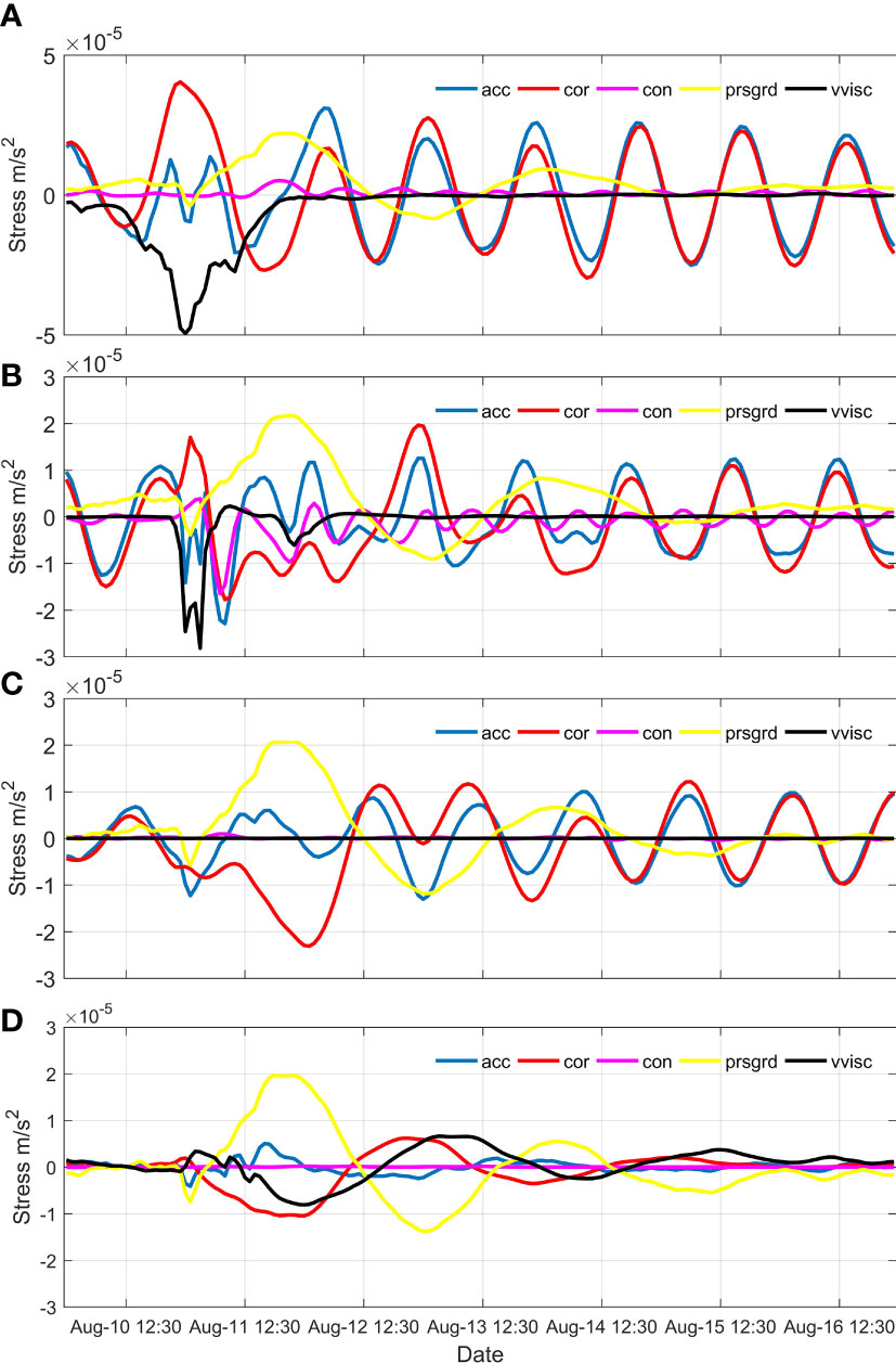
Figure 13 Diagnostic analysis in the different layers at the mooring site. (A) Surface layer. (B) Thermocline. (C) Lower mixing layer. (D) Bottom boundary layer. The blue, red, magenta, yellow, and black lines represent the term of acceleration, the Coriolis force, convection, pressure gradient force, and viscosity term, respectively.

FIGURE 14

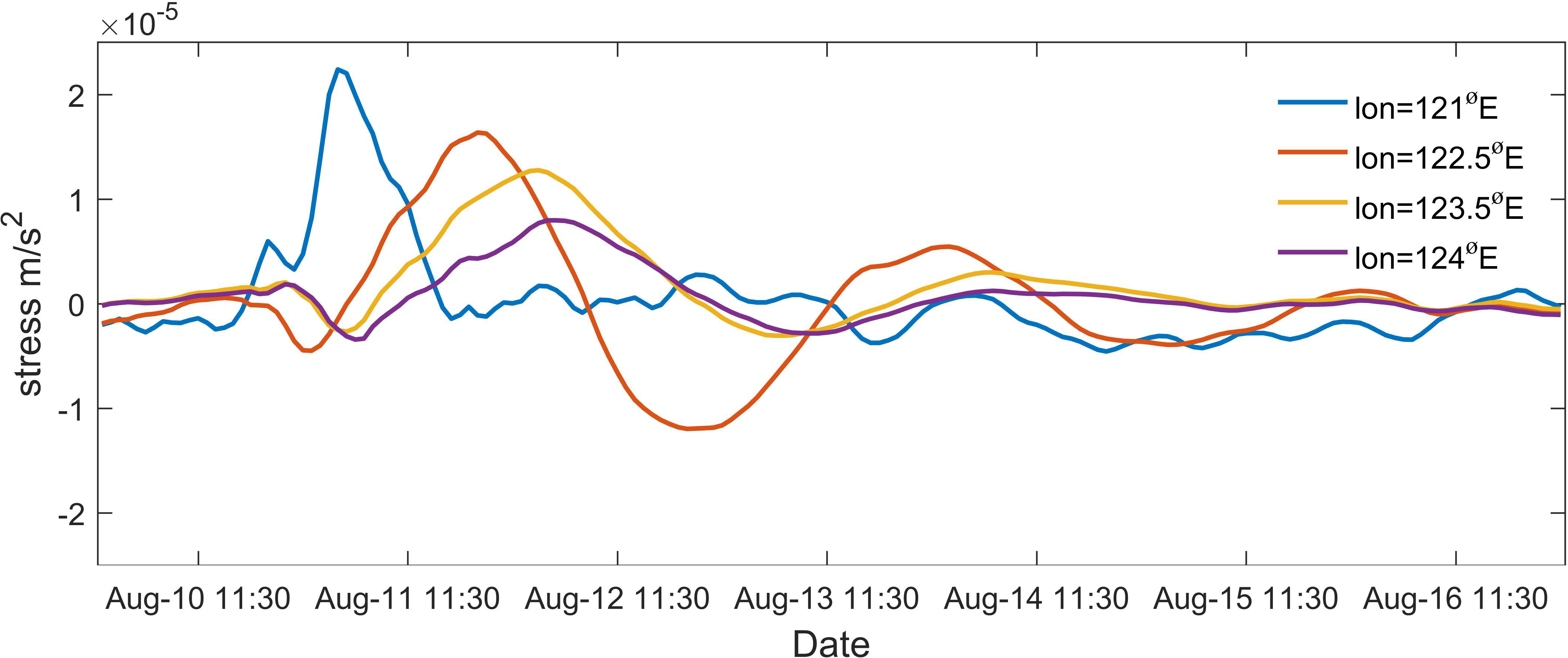
Figure 14 Time plot of pressure gradient force (m/s²) at different longitude of 34°N. The blue, orange, yellow, and purple lines represent variation of pressure gradient forces with time at 121°E, 122.5°E, 123.5°E, and 124°E of 34°N, respectively.

Below the mixed layer, the seawater began to respond to the pressure gradient force at 12:00 on 11^th August, promoting the evident variation in the terms of acceleration, Coriolis force, convection, and eddy viscosity (Figures 13B–D). In the strongly stratified thermocline, although the near-inertial wave was generated, it was not evident in the observations and model. Strong nonlinear phenomena were observed in the thermocline by Davies (2005), suggesting that the enhancement of the convection term contributes to a cascade of near-inertial energy to smaller scales, as a result of the weakening of the near-inertial energy. It can be clarified that the convection term (magenta line in Figure 13B), owing to velocity shear increased to the same magnitude as Coriolis force around 12:00 on 11^th August and balanced part of the pressure gradient force, resulting in a reduction in the near-inertial flow. The terms of acceleration, vertical advection, and Coriolis force together balanced the pressure gradient force. It is worth noting that the convective term caused by velocity shear only appears in the thermocline, which is the main reason for the weakening of near-inertial flow in the thermocline.

In the lower mixed layer, the motion of seawater is driven by pressure gradient force, which is balanced only by acceleration and Coriolis forces together (Figure 13C). Therefore, this motion behaves as a near-inertial motion and the near-inertial flow was greater than that in the thermocline, owing to the fact that it is not modulated by the advection term. After the disappearance of the pressure gradient force, the motion evolves into inertial motion.

At the boundary layer, a portion of the pressure gradient force was balanced by the eddy viscosity (black line in Figure 13D), resulting in the rapid decrease in the near-inertial velocity relative to that in the lower mixed layer. Thus, the two velocity peaks occur in the upper and lower mixed layers, and the weak inertial velocities in the thermocline and bottom boundary layers are influenced by the convective and eddy viscosity terms respectively.

4 Conclusions

Based on observations and numerical simulations, a typical near-inertial motion caused by a cyclonic wind field was investigated and its dynamical processes were characterised in the YS. With the arrival of the cyclone, the temperature of the mixed layer decreased and the depth of the mixed layer deepened, leading to the compression of the thermocline and the strengthening of the stratification. Near-inertial velocity reached a peak value of 0.15 m/s with a phase difference of 180° in the mixed layer and below the thermocline. The dominant first mode derived from wind energy caused the strongest shear at the thermocline, where intense stratification inhibited the development of shear instability. However, sub-shear peak resulting from the higher mode and weak stratification led to the development of shear instability below the thermocline. In the coastal region with homogeneous seawater, near-inertial energy was weak relative to that in the offshore region. In shelf-stratified seas, the near-inertial energy in the surface layer was mainly associated with the wind energy input, whereas the near-inertial flow below the thermocline was related to that in the mixed layer and the water depth below the thermocline to satisfy cross-shelf flux conservation.

Tides change the vertical structure of the near-inertial flow by altering the magnitude and distribution of the eddy viscosity. In conditions without tides, the near-inertial velocity decreased significantly within the bottom 10m, corresponding to a strong eddy viscosity. When considering the influence of tides, the near-inertial velocity decreased significantly from the a depth of 20m to the seafloor.

The response of the ocean to time-varying wind fields first appears in the mixed layer. During the forcing phase, the wind drives the movement of the upper layer of seawater, causing it to accumulate at the shore. During the relaxation phase of the wind stress disappearance, the accumulated seawater is released at the shore and forms a barotropic wave that propagates offshore. When the barotropic wave arrived, near-inertial oscillations were formed below the thermocline in the opposite phase to that in the mixed layer by the driving of the pressure gradient force. Within the thermocline, the near-inertial flow is weaker owing to the strong convection term balancing part of the pressure gradient force. Within the bottom boundary layer, the eddy viscosity term balances the partial pressure gradient force, resulting in a rapid reduction of the near-inertial flow. Therefore, two peaks of near-inertial flow velocity occur in the mixed layer and below the thermocline.

Data availability statement

The raw data supporting the conclusions of this article will be made available by the authors, without undue reservation.

Author contributions

YH designed and wrote the manuscript. FY contributed to the designed test and revision of the manuscript and supervised manuscripts. ZC participated in the revision of the manuscript.GS and XL provided some suggestions for ROMS configuration. FN provided some ideas and QR gave some supporting data. All authors contributed to the article and approved the submitted version.

Funding

This work is supported by the Strategic Priority Program of Chinese Academy of Sciences (grant number XDA19060201).

Acknowledgments

We thank the technology support provided by the High Performance Computing Center, Institute of Oceanology, Chinese Academy of Sciences.

Conflict of interest

The authors declare that the research was conducted in the absence of any commercial or financial relationships that could be construed as a potential conflict of interest.

Publisher’s note

All claims expressed in this article are solely those of the authors and do not necessarily represent those of their affiliated organizations, or those of the publisher, the editors and the reviewers. Any product that may be evaluated in this article, or claim that may be made by its manufacturer, is not guaranteed or endorsed by the publisher.

References

Alford M. H. (2001). Internal swell generation: The spatial distribution of energy flux from the wind to mixed layer near-inertial motions. J. Phys. Oceanogr 31 (8), 2359–2368. doi: 10.1175/1520-0485(2001)031<2359:Isgtsd>2.0.Co;2

CrossRef Full Text | Google Scholar

Alford M. H., MacKinnon J. A., Simmons H. L., Nash J. D. (2016). Near-inertial internal gravity waves in the ocean. Annu. Rev. Mar. Sci. 8, 95–123. doi: 10.1146/annurev-marine-010814-015746

CrossRef Full Text | Google Scholar

Anderson I., Huyer A., Smith R. L. (1983). Near-inertial motions off the Oregon coast. J. Geophys Res-Oceans 88 (Nc10), 5960–5972. doi: 10.1029/JC088iC10p05960

CrossRef Full Text | Google Scholar

Bi C. C., Yao Z. G., Bao X. W., Zhang C., Ding Y., Liu X. H., et al. (2021). The sensitivity of numerical simulation to vertical mixing parameterization schemes: A case study for the yellow Sea cold water mass. J. Oceanol Limnol 39 (1), 64–78. doi: 10.1007/s00343-019-9262-y

CrossRef Full Text | Google Scholar

Chen S. L., Chen D. Y., Xing J. X. (2017). A study on some basic features of inertial oscillations and near-inertial internal waves. Ocean Sci. 13 (5), 829–836. doi: 10.5194/os-13-829-2017

CrossRef Full Text | Google Scholar

Chen C. S., Reid R. O., Nowlin W. D. (1996). Near-inertial oscillations over the Texas Louisiana shelf. J. Geophys Res-Oceans 101 (C2), 3509–3524. doi: 10.1029/95jc03395

CrossRef Full Text | Google Scholar

Chen C. S., Xie L. S. (1997). A numerical study of wind-induced, near-inertial oscillations over the Texas-Louisiana shelf. J. Geophys Res-Oceans 102 (C7), 15583–15593. doi: 10.1029/97jc00228

CrossRef Full Text | Google Scholar

Davies A. M. (1985). A 3 dimensional modal model of wind induced flow in a Sea region. Prog. Oceanogr 15 (2), 71–128. doi: 10.1016/0079-6611(85)90032-1

CrossRef Full Text | Google Scholar

Davies A. M., Xing J. X. (2003). On the interaction between internal tides and wind-induced near-inertial currents at the shelf edge. J. Geophys Res-Oceans 108 (C3), 3099. doi: 10.1029/2002jc001375

CrossRef Full Text | Google Scholar

Davies A. M., Xing J. X. (2005). The effect of a bottom shelf front upon the generation and propagation of near-inertial internal waves in the coastal ocean. J. Phys. Oceanogr 35 (6), 976–990. doi: 10.1175/Jpo2732.1

CrossRef Full Text | Google Scholar

Gill. (1982). Atmosphere-ocean dynamics. (Academic) 662.

Google Scholar

Hao J. J., Chen Y. L., Wang F., Lin P. F. (2012). Seasonal thermocline in the China seas and northwestern pacific ocean. J. Geophys Res-Oceans 117. doi: 10.1029/2011jc007246

CrossRef Full Text | Google Scholar

Hisaki Y., Naruke T. (2003). Horizontal variability of near-inertial oscillations associated with the passage of a typhoon. J. Geophys Res-Oceans 108 (C12). doi: 10.1029/2002jc001683

CrossRef Full Text | Google Scholar

Jacob S. D., Shay L. K., Mariano A. J., Black P. G. (2000). The 3D oceanic mixed layer response to hurricane Gilbert. J. Phys. Oceanogr 30 (6), 1407–1429. doi: 10.1175/1520-0485(2000)030<1407:Tomlrt>2.0.Co;2

CrossRef Full Text | Google Scholar

Kelly S. M. (2019). Coastally generated near-inertial waves. J. Phys. Oceanogr 49 (11), 2979–2995. doi: 10.1175/Jpo-D-18-0148.1

CrossRef Full Text | Google Scholar

Kundu P. K. (1976). Analysis of inertial oscillations observed near Oregon coast. J. Phys. Oceanogr 6 (6), 879–893. doi: 10.1175/1520-0485(1976)006<0879:Aaoioo>2.0.Co;2

CrossRef Full Text | Google Scholar

Kunze E. (1985). Near-inertial wave-propagation in geostrophic shear. J. Phys. Oceanogr 15 (5), 544–565. doi: 10.1175/1520-0485(1985)015<0544:Niwpig>2.0.Co;2

CrossRef Full Text | Google Scholar

Large W. G., Pond S. (1981). Open ocean momentum flux measurements in moderate to strong winds. J. Phys. Oceanogr 11 (3), 324–336. doi: 10.1175/1520-0485(1981)011<0324:Oomfmi>2.0.Co;2

CrossRef Full Text | Google Scholar

Lee J. H., Pang I. C., Moon J. H. (2016). Contribution of the yellow Sea bottom cold water to the abnormal cooling of sea surface temperature in the summer of 2011. J. Geophys Res-Oceans 121 (6), 3777–3789. doi: 10.1002/2016jc011658

CrossRef Full Text | Google Scholar

Lewis J. K. (2001). Cross-shelf variations of near-inertial current oscillations. Cont Shelf Res. 21 (5), 531–543. doi: 10.1016/S0278-4343(00)00092-3

CrossRef Full Text | Google Scholar

Li R. X., Chen C. S., Dong W. J., Beardsley R. C., Wu Z. X., Gong W. P., et al. (2021). Slope-intensified storm-induced near-inertial oscillations in the south China Sea. J. Geophys Res-Oceans 126 (3). doi: 10.1029/2020JC016713

CrossRef Full Text | Google Scholar

Li J. C., Li G. X., Xu J. S., Dong P., Qiao L. L., Liu S. D., et al. (2016). Seasonal evolution of the yellow Sea cold water mass and its interactions with ambient hydrodynamic system. J. Geophys Res-Oceans 121 (9), 6779–6792. doi: 10.1002/2016jc012186

CrossRef Full Text | Google Scholar

Liu Z. Y., Wei H., Lozovatsky I. D., Fernando H. J. S. (2009). Late summer stratification, internal waves, and turbulence in the yellow Sea. J. Mar. Syst. 77 (4), 459–472. doi: 10.1016/j.jmarsys.2008.11.001

CrossRef Full Text | Google Scholar

Lu X., Zhang J. (2006). Numerical study on the spatially varying bottom friction coefficient of a 2D tidal model with adjoint method. Continent. Shelf Res. 26 (16), 1905–23. doi: 10.1016/j.scr.2006.06.007

CrossRef Full Text | Google Scholar

MacKinnon J. A., Gregg M. C. (2005). Near-inertial waves on the new England shelf: The role of evolving stratification, turbulent dissipation, and bottom drag. J. Phys. Oceanogr 35 (12), 2408–2424. doi: 10.1175/Jpo2822.1

CrossRef Full Text | Google Scholar

Malone F. D. (1968). An analysis of current measurements in lake Michigan. J. Geophys Res. 73 (22), 7065. doi: 10.1029/JB073i022p07065

CrossRef Full Text | Google Scholar

Meng Q. J., Li P. L., Zhai F. G., Gu Y. Z. (2020). The vertical mixing induced by winds and tides over the yellow Sea in summer: A numerical study in 2012. Ocean Dynam 70 (7), 847–861. doi: 10.1007/s10236-020-01368-2

CrossRef Full Text | Google Scholar

Millot C., Crépon M. (1981). Inertial oscillations on the continental-shelf of the gulf of lions - observations and theory. J. Phys. Oceanogr 11 (5), 639–657. doi: 10.1175/1520-0485(1981)011<0639:Iootcs>2.0.Co;2

CrossRef Full Text | Google Scholar

Moon I. J., Kwon S. J. (2012). Impact of upper-ocean thermal structure on the intensity of Korean peninsular landfall typhoons. Prog. Oceanogr 105, 61–66. doi: 10.1016/j.pocean.2012.04.008

CrossRef Full Text | Google Scholar

Mukherjee A., Shankar D., Aparna S. G., Amol P., Fernando V., Fernandes R., et al. (2013). Near-inertial currents off the east coast of India. Cont Shelf Res. 55, 29–39. doi: 10.1016/j.csr.2013.01.007

CrossRef Full Text | Google Scholar

Munk W., Wunsch C. (1998). Abyssal recipes II: Energetics of tidal and wind mixing. Deep-Sea Res. Pt I 45 (12), 1977–2010. doi: 10.1016/S0967-0637(98)00070-3

CrossRef Full Text | Google Scholar

Oh K. H., Lee S., Song K. M., Lie H. J., Kim Y. T. (2013). The temporal and spatial variability of the yellow Sea cold water mass in the southeastern yellow Se-2011. Acta Oceanol Sin. 32 (9), 1–10. doi: 10.1007/s13131-013-0346-9

CrossRef Full Text | Google Scholar

Pawlowicz R., Beardsley B., Lentz S. (2002). Classical tidal harmonic analysis including error estimates in MATLAB using T-TIDE. Comput. Geosci-Uk 28 (8), 929–937. doi: 10.1016/S0098-3004(02)00013-4

CrossRef Full Text | Google Scholar

Qiao F. L., Ma J., Xia C. S., Yang Y. Z., Yuan Y. L. (2006). Influences of the surface wave-induced mixing and tidal mixing on the vertical temperature structure of the yellow and East China seas in summer. Prog. Nat. Sci. 16 (7), 739–746.

Google Scholar

Rubio A., Reverdin G., Fontan A., Gonzalez M., Mader J. (2011). Mapping near-inertial variability in the SE bay of Biscay from HF radar data and two offshore moored buoys. Geophys Res. Lett. 38. doi: 10.1029/2011gl048783

CrossRef Full Text | Google Scholar

Shchepetkin A. F., McWilliams J. C. (2005). The regional oceanic modeling system (ROMS): A split-explicit, free-surface, topography-following-coordinate oceanic model. Ocean Model. 9 (4), 347–404. doi: 10.1016/j.ocemod.2004.08.002

CrossRef Full Text | Google Scholar

Shearman R. K. (2005). Observations of near-inertial current variability on the New England shelf. J. Geophys. Res. 110 (C2). doi: 10.1029/2004jc002341

CrossRef Full Text | Google Scholar

Sobarzo M., Shearman R. K., Lentz S. (2007). Near-inertial motions over the continental shelf off concepcion, central Chile. Prog. Oceanogr 75 (3), 348–362. doi: 10.1016/j.pocean.2007.08.021

CrossRef Full Text | Google Scholar

Song D. H., Gao G. D., Xia Y. Y., Ren Z. P., Liu J. L., Bao X. W., et al. (2021). Near-inertial oscillations in seasonal highly stratified shallow water. Estuar. Coast. Shelf S 258. doi: 10.1016/j.ecss.2021.107445

CrossRef Full Text | Google Scholar

Song D., Wang X. H., Cao Z., Guan W. (2013). Suspended sediment transport in the Deepwater Navigaation Channel, Yangtze River Estuary, China, in the dry season 2009: 1. Observations over spring and neap tidal cycles. J. Geophys. Res. 180 (10), 5555–5567. doi: 10.1002/jgrc.20410

CrossRef Full Text | Google Scholar

Thorne P. D., Hurther D. (2014). An overview on the use of backscattered sound for measuring suspended particle size and concentration profiles in non-cohesive inorganic sediment transport studies. Cont Shelf Res. 73, 97–118. doi: 10.1016/j.csr.2013.10.017

CrossRef Full Text | Google Scholar

Thorpe S. A., Jiang R. (1998). Estimating internal waves and diapycnal mixing from conventional mooring data in a lake. Limnol Oceanogr 43 (5), 936–945. doi: 10.4319/lo.1998.43.5.0936

CrossRef Full Text | Google Scholar

Tintore J., Wang D. P., Garcia E., Viudez A. (1995). Near-inertial motions in the coastal ocean. J. Mar. Syst. 6 (4), 301–312. doi: 10.1016/0924-7963(94)00030-F

CrossRef Full Text | Google Scholar

Wan Z., Qiao F., Yuan Y. (1998). Three-dimensional numerical modelling of tidal waves in the bohai, yellow and East China seas. Oceanologia Limnologia Sin. 29 (6), 611–616.

Google Scholar

Xia Y. Y., Bao X. W., Song D. H., Ding Y., Wan K., Yan Y. H. (2019). Tidal effects on the bottom thermal front of north yellow Sea cold water mass near zhangzi island in summer 2009. J. Ocean U China 18 (4), 751–760. doi: 10.1007/s11802-019-3892-8

CrossRef Full Text | Google Scholar

Xia C. S., Qiao F. L., Yang Y. Z., Ma J., Yuan Y. L. (2006). Three-dimensional structure of the summertime circulation in the yellow Sea from a wave-tide-circulation coupled model. J. Geophys Res-Oceans 111 (C11). doi: 10.1029/2005jc003218

CrossRef Full Text | Google Scholar

Yang B., Hou Y. J., Hu P., Liu Z., Liu Y. H. (2015). Shallow ocean response to tropical cyclones observed on the continental shelf of the northwestern south China Sea. J. Geophys Res-Oceans 120 (5), 3817–3836. doi: 10.1002/2015jc010783

CrossRef Full Text | Google Scholar

Yang Y., Li K. P., Du J. T., Liu Y. L., Liu L., Wang H. W., et al. (2019). Revealing the subsurface yellow Sea cold water mass from satellite data associated with typhoon muifa. J. Geophys Res-Oceans 124 (10), 7135–7152. doi: 10.1029/2018jc014727

CrossRef Full Text | Google Scholar

Yu F., Zhang Z. X., Diao X. Y., Guo J. S., Tang Y. X. (2006). Analysis of evolution of the huanghai Sea cold water mass and its relationship with adjacent water masses. Acta Oceanologica Sin. 28, 26–34.

Google Scholar

Zhai X. M. (2017). Dependence of energy flux from the wind to surface inertial currents on the scale of atmospheric motions. J. Phys. Oceanogr 47 (11), 2711–2719. doi: 10.1175/Jpo-D-17-0073.1

CrossRef Full Text | Google Scholar

Zhang S. W., Wang Q. Y., Lu Y., Cui H., Yuan Y. L. (2008). Observation of the seasonal evolution of the yellow Sea cold water mass in 1996-1998. Cont Shelf Res. 28 (3), 442–457. doi: 10.1016/j.csr.2007.10.002

CrossRef Full Text | Google Scholar

Zhang H., Zhu J. R., Wu H. (2005). Numerical simulation of eight main tidal constituents in the East China Sea, yellow Sea and bohai Sea. J. East China Normal Univ. (Natural Science) 3), 71–77.

Google Scholar