Fortnightly variability of horizontal salinity gradient affects exchange flow in the Sumjin River estuary

The horizontal salinity gradient has been reported to play a crucial role in fortnightly variability of estuarine exchange flow in short estuaries. However, spatiotemporal variations in the salinity gradient and exchange flow have not been examined over an entire short estuary, as only data observed only at specific points was available. We analyzed the variation in salinity gradient along the entire Sumjin River estuary and its effect on the exchange flow over fortnightly tidal cycles based on observations and numerical model experiments. The salinity gradient and exchange flow were in different phases between the lower and upper estuaries by 6–7 days. The maximum salinity gradient periodically reciprocated along the channel as a result of salt flux changes determined by vertical mixing. The stronger exchange flow (> 0.04 m s^-1) changed location from mouth to head of estuary while the tidal range decreased, resulting from variability of the salinity gradient. The horizontal salinity gradient is large enough to overwhelm the vertical mixing effect on the exchange flow. The spatiotemporal changes of strong exchange flow correspond well with the horizontal Richardson number value (> 3). This study suggests that for the health of estuarine ecosystems, it is important to determine the spatiotemporal variation in exchange flow throughout the estuary.

Introduction

The transport and behavior of substances, such as pollutant sediments, organisms, and nutrients, largely depend on the strength of estuarine exchange flow. The exchange flow is the tidally averaged along-channel velocity through an estuarine cross-section (Stacey et al., 2001; Valle-Levinson, 2010; Geyer and MacCready, 2014) and is also referred to as estuarine circulation (Geyer and MacCready, 2014; Dijkstra et al., 2017). The vertical shear of the exchange flow is mainly determined by competition between vertical mixing and the horizontal salinity gradient (Uncles and Stephens, 1990; Park and Kuo, 1996; Stacey et al., 2001; Mantovanelli et al., 2004; Valle-Levinson, 2010; Garel and Ferreira, 2013). Increased vertical mixing enhances the vertical momentum flux, which weakens the vertical shear of exchange flow, whereas an increased salinity gradient strengthens the vertical shear. The intensity of vertical mixing and salinity gradient can vary depending on the tidal range, and the contention results of these two factors change fortnightly; in turn, this determines exchange flow (Park and Kuo, 1996).

Previous studies have proposed that fortnightly variation in the vertical shear of exchange flow is determined by turbulent mixing owing to the tide. During spring tides, vertical momentum exchange is active owing to strong vertical mixing, and exchange flow is weakened; during the neap tide, exchange flow is strong owing to decreased vertical mixing, as observed in many estuaries, such as the Hudson River estuary (Geyer et al., 2000; Bowen and Geyer, 2003; Scully et al., 2009; MacCready and Geyer, 2010), Modaomen estuary (Gong et al., 2014), Peruípe River estuary (Andutta et al., 2013), and Curimatau River estuary (de Miranda et al., 2005). On the other hand, recent studies of short estuaries (i.e., those that are shorter than the dominant tidal wavelength) have reported that the salinity gradient plays a major role in the exchange flow variation, which is stronger during the spring tide (Becker et al., 2009; Cho et al., 2020). In the Cape Fear River estuary, stronger tidal forcing and associated mixing contribute to increased estuarine circulation due to a greater near-bottom horizontal salinity gradient during the high tidal range (Becker et al., 2009). In the Sumjin River estuary, the effect of the horizontal salinity gradient, which is six times higher during the spring tide compared with the neap tide, overwhelms the effect of vertical mixing, resulting in stronger exchange flow during the spring tide (Cho et al., 2020). However, as these studies were conducted only at specific points, the fortnightly variation of exchange flow over the whole short estuary remains unclear. In the study of the short Blackwater estuary, a semi-analytical approach was used and the analysis focused on lateral changes in residual circulation, but did not examine spring–neap variation (Wei et al., 2022). Therefore, fortnightly variation of the vertical shear of exchange flow in the entire estuary is still poorly understood as the analysis has received little attention.

In this study, the variability of the horizontal salinity gradient and exchange flow during the fortnightly tidal cycle was analyzed for the entire short and narrow estuary, based on observations and numerical model experiments. The estuary was simulated using a numerical model by simplifying the geometry of the Sumjin River estuary. The mechanism underlying periodic salinity gradient change and its effect on the exchange flow were investigated. A numerical experiment with realistic topography was conducted to examine its applicability to the Sumjin River estuary.

Materials and methods

Study area

The Sumjin River estuary is located in the central part of the southern coast of Korea (Figure 1A). The Sumjin River discharges into Gwangyang Bay (Figure 1B). The Sumjin River discharges into Gwangyang Bay. The length of the estuary is estimated to be approximately 25 km based on the salinity distribution suggested by Pritchard (1967). The scale of the estuary can be classified by a non-dimensional length parameter (δ), which is the ratio between the length of the estuary (L) and one-quarter of the tidal wavelength (λ/4), according to the definition of Li and O’Donnell (2005) as follows:

$\begin{array}{ll}\mathbf{\delta }\mathbf{=}\frac{\mathbf{4}\mathbf{L}}{\mathbf{\lambda }} \mathbf{\left(}\mathbf{\lambda }\mathbf{=}\frac{\sqrt{\mathbf{g}\mathbf{h}}}{\mathbf{f}}\mathbf{\right)}\mathbf{,} & (1)\end{array}$

where g is the acceleration of gravity, h is the depth, and f is the tidal frequency (2.23×10^-5 s^-1). An estuary with a δ value smaller (or larger) than 0.6–0.7 is defined as a short (or long) estuary. The Sumjin River estuary, has a δ value of 0.27 and can therefore be classified as a short estuary. The estuary is relatively a narrow and shallow estuary; the width and depth at the mouth are 1 km and 15 m, respectively, decreasing to 300 m and 2 m at the head. There are tributaries on the lower estuary side. However, based on data from Conductivity–Temperature–Depth (CTD) station 7, the east tributary has minimal effect on the salinity distribution of the main channel. A tributary on the west from station 4 has flow mainly out of the estuary, with hardly any flow into the estuary.

The tides are mainly mixed semi-diurnal, and the main tidal constituents are M₂ and S₂, with amplitudes of ~1 and ~0.46 m, respectively. These two tidal components were used as forcing in the model. The tidal range is approximately 3.1 m during the spring tide and 1.0 m during the neap tide. Estuary stratification is partially to well mixed during spring tides and becomes stratified during neap tides (Shaha and Cho, 2009), and it is periodically strongly stratified. Tidal data were collected from the Gwangyang tidal gauge station, which is operated by the Korea Hydrographic and Oceanographic Agency (http://www.khoa.go.kr). The 20-year mean discharge rate of the Sumjin River from 2001 to 2020 was 78 m³ s^-1. The river discharge rate was obtained from the Songjung gauge station, which is located approximately 35 km upstream of the estuary mouth and is operated by the Ministry of Construction and Transportation (http://www.wamis.go.kr).

Observations

We observed the current velocity at one point and salinity at 12 stations along the channel up to 12 km upstream from the mouth of estuary. The velocity was observed by upward-looking Recording Doppler Current Profiler (RDCP 600 kHz; Aanderaa Data Instruments AS, https://www.aanderaa.com/) for 23 days at 7 km upstream from the mouth of estuary (Figure 1B; RDCP). The upward-looking RDCP was installed at the deepest point (12 m) in the section to obtain vertical velocity profiles from October 19 to November 10, 2013. The velocity data were obtained at 10-min intervals with a vertical resolution of 1 m from 3 m above the bottom to the surface layer. The upper and lower most bins were excluded to avoid boundary interference. The north and east components of the velocities were decomposed to obtain along- and cross-channel velocities; the along-channel velocity was analyzed in this study.

FIGURE 1

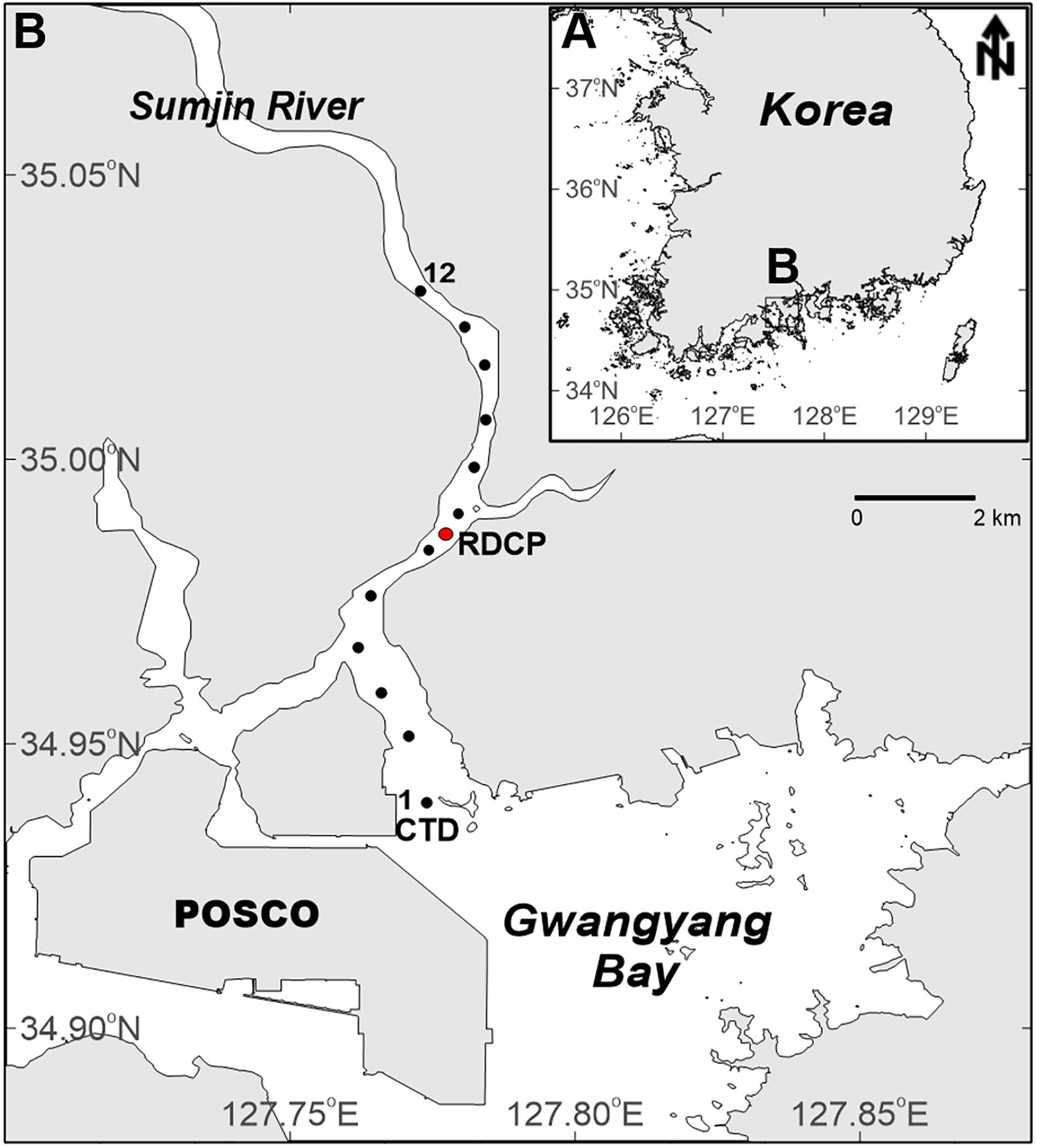
Figure 1 Study area and observation stations: (A) Overview map of Korea; (B) the Sumjin River estuary, including the Conductivity–Temperature–Depth (CTD) stations 1–12 (black circles), the current mooring station (red circle), and the Gwangyang tidal gauge (triangle).

The YSI Castaway Conductivity–Temperature–Depth (CTD) (https://www.sontek.com/castaway-ctd) was used during shipboard surveys conducted on a neap tide (October 30, 2013) and spring tide (November 5, 2013). Hydrological data were acquired along the estuary from stations 1–12 (Figure 1B), with an accuracy of 0.1 g kg^-1 for salinity and 0.05°C for temperature. The distance between the stations was approximately 1 km. The CTD observations started from station 1, 30 min before the peaks of the flood and ebb tides. The observations up to station 12 usually took less than 50 min to minimize the total casting time to maintain the concurrence of the tidal phase along the estuary. The subtidal salinity was calculated by averaging the flood and ebb observations. More detailed information regarding these observations is described in Cho et al. (2020).

Model description

We assumed a simplified Sumjin River estuary system that is well mixed or periodically stratified, forced with a steady river flow rate and two tidal constituents (M₂, S₂), resulting in fortnightly tidal variation. This particular configuration was designed to be as simple as possible in order to reproduce the spring–neap tidal variation observed in the Sumjin River estuary. The simulation was performed using the Regional Ocean Modeling System (ROMS), which solves the hydrostatic, incompressible, Reynolds-averaged momentum and tracer conservation equations with a terrain-following vertical coordinate and free surface (Shchepetkin and McWilliams, 2005).

The idealized model domain includes a bay between the open boundary and estuary mouth (Figure 2A). To match the observations, we assumed that the estuary mouth was located 7 km from the boundary. The estuary was implemented in a straight line to exclude the effect of meandering. The cross-section was rectangular in shape, and the water depth and width followed a linear trend based on the actual change (Figures 2B, C). This simplification minimizes the nonlinear effect caused by complex topography and focuses only on the fortnightly variation. However, since these settings are different from the friction effect in real geometry, the mixing parameterization should be elaborately tuned using a proper vertical mixing scheme and forcing. The vertical mixing was parameterized using the K-Profile Parameterization scheme (KPP; Large et al., 1994). In the Mellor–Yamada and GLS (k-kl, k-e, k-w) mixing schemes, the thickness of the thermocline was thinner than that of the KPP during the neap tide, and the length of inflow of the high salinity (> 28) water mass to the bottom layer was longer by 1–5 km. During the spring tide, all schemes similarly implemented strong vertical mixing, but in all schemes other than KPP, the inflow of the high salinity water mass was longer by 1–4 km. The vertically averaged salinity reduction rate along the channel and the inflow length of high salinity water were most similar to the observation in the KPP.

FIGURE 2

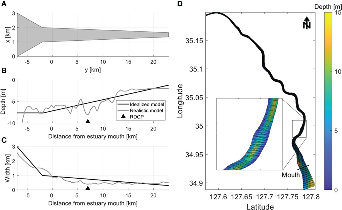
Figure 2 Idealized model domain information. (A) Idealized estuary model domain and the along-channel variations of (B) depth and (C) width for the model (black lines) and observations (grey lines) in the Sumjin River estuary. The observation depth is laterally averaged. The black triangles indicate the velocity observation station in Figure 1B RDCP. (D) Realistic model domain with depth (m); the estuary mouth is indicated by the black line.

The idealized model was constructed with 110 (along-channel, y-direction) × 17 (cross-channel, x-direction) grids and 10 (vertical, z-direction) vertical layers. The along-channel grid size (Δy) was 340 m, the cross-channel grid size (Δx) was 34–190 m, and the 10 vertical layers were uniformly discretized. The model was forced by river flow at the northern end of the estuarine channel, and two tidal components were imposed at the southern boundary. The inflowing river discharge rate was 60 m³ s^-1, with a salinity of 0 g kg^-1, which was suitable for an idealized model. The salinity at the ocean boundary was 35 g kg^-1, and the initial salinity was set to 20 g kg^-1. The temperatures at the open boundary and river inflow were set to 20°C, the same as the background temperature set throughout the entire domain. The open boundary was treated with the Champman condition for surface elevation, Flather condition for barotropic velocity, and Clamped boundary conditions for open-ocean salinity. The other forcing was a tidal sea surface height variation on the open boundaries at the M₂ and S₂ frequencies. The idealized model was integrated for 100 days with a baroclinic time step of 10 s. The idealized model presented a steady spring–neap tidal cycle in the salinity field after a spin-up period of 30 days, after which it was run for another 70 days to capture several fortnightly tidal cycles.

The realistic model was constructed with 158 (along-channel, y-direction) × 14 (cross-channel, x-direction) grids and 10 (vertical, z-direction) vertical layers (Figure 2D). The along-channel grid size (Δy) was 10–540 m, the cross-channel grid size (Δx) was 6–240 m, and the 10 vertical layers were uniformly discretized. Like the idealized model, the realistic model was forced by river flow and the two tidal components at the northern and southern boundary, respectively. The initial and boundary values of salinity and water temperature were also the same as in the idealized model. The realistic model was integrated for 100 days with a baroclinic time step of 2 s. The realistic model presented a steady spring–neap tidal cycle in the salinity field after a spin-up period of 30 days, after it had been run for another 70 days to capture several fortnightly tidal cycles.

Comparison of salinity and current between observations and models

The model was designed to simulate the fortnightly variability of salt distribution in the Sumjin River estuary, and the results were compared with the observations. The salinity in the model was in good agreement with that observed at most stations (Figure 3). The root-mean-square error for all the stations in idealized (realistic) model was 0.68 (3.4) and 0.48 (1.68) g kg^-1 for depth-averaged salinity along the channel and 0.51 (0.46) and 0.35 (0.48) km^-1 for the horizontal salinity gradient during the spring and neap tides, respectively. Model salinity sections were vertically mixed as observed during the spring tide, but stratified more strongly than observed during the neap tide. However, both models reproduced accurately that the salinity gradient was up to 7 times greater during the spring than the neap tide, which was a major feature in observation.

FIGURE 3

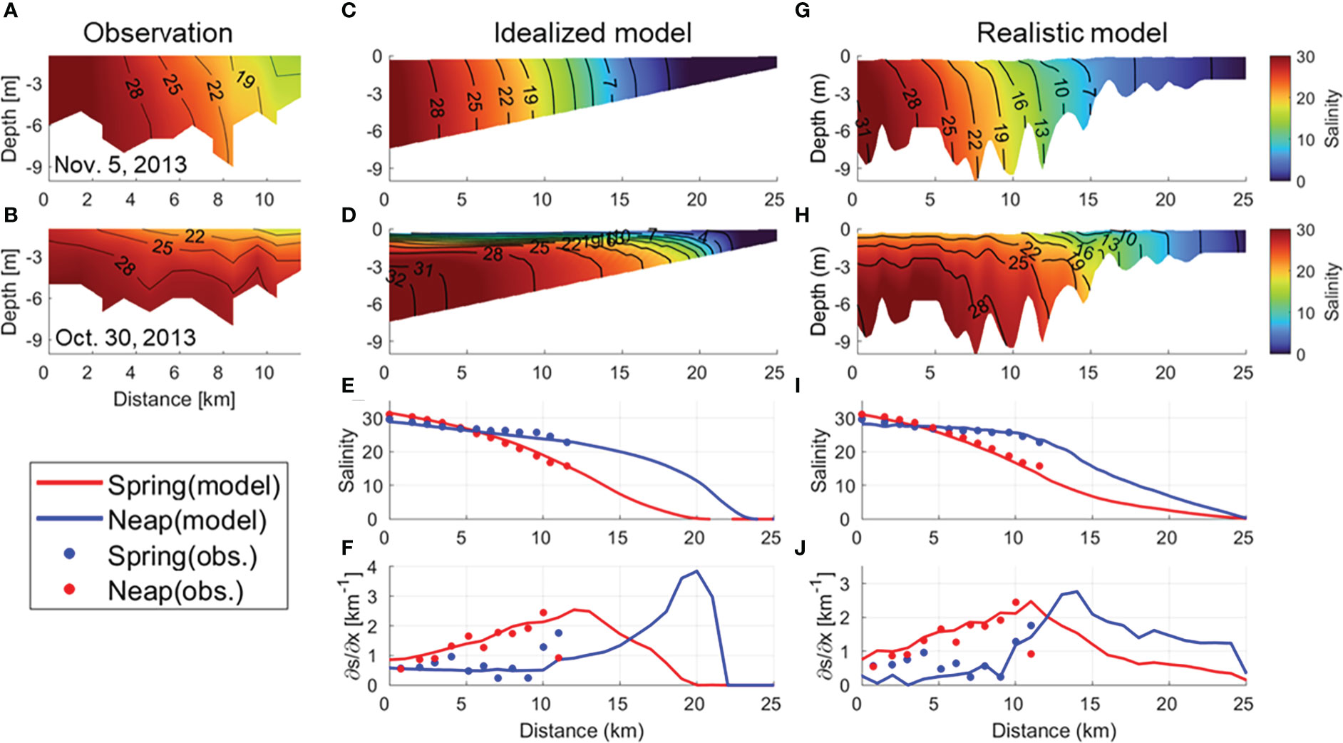
Figure 3 Comparisons of salinity among observations, an idealized model, and a realistic model. Vertical sections of the along-channel salinity during (A, C, G) the spring tide and (B, D, H) neap tide in (A, B) observations, (C, D) the idealized model and (G, H), and the realistic model. Variations in depth-averaged (E, I) salinity and (F, J) horizontal salinity gradient from mouth to head during spring (red) and neap tides (blue). Dots and lines denote observations and model outputs, respectively.

The horizontal salinity gradient may vary depending on the horizontal length scale (Geyer et al., 2000) and the depth to be used. Therefore, we needed to check whether there was a change in the fortnightly variation of the salinity gradient. So, when calculating the salinity gradient with the observed salinity, the horizontal length was changed to 1–10 km intervals. When the salinity was averaged vertically, the water depth from the surface layer was also applied differently. As the horizontal interval increased, the horizontal salinity difference also increased, and the salinity gradient decreased only slightly. Even when the salinity gradient was estimated by averaging the salinity at various water depths, there was almost no change. In the analytical model using the balance equation of pressure gradient and friction (Cho et al., 2020), the observed exchange flow was well realized when the horizontal length scale was set at a 1 km interval when calculating the salinity gradient. Therefore, we used the salinity from the surface layer to the bottom and set the horizontal length to 1 km to calculate the salinity gradient.

A comparison of the depth-averaged along-channel velocity between the model and the observations indicated that the phase was properly simulated; however, the magnitude was overpredicted in the model (Figure 4A). When the tidal range was small, the difference in magnitude was approximately 15 cm s^-1, which decreased to 7 cm s^-1 at a large tidal range. The exchange flow in observations and the model was compared (Figure 4B). The exchange flow was calculated using a 25-hour low pass filter (MATLAB R2021b function: all subsequent low pass filter used this tool) for the observation results at a 10 min interval, and for the model at a 1-hour interval to suppress semi-diurnal tidal variability. We tried different timeframes (25 – 72 h) for the low pass filters, and the results were all similar. The vertical shear of the exchange flow observed at the lower estuary was greater during spring tides than during neap tides (Figure 4B). The model captured the difference in the vertical velocity profile between the two periods well.

FIGURE 4

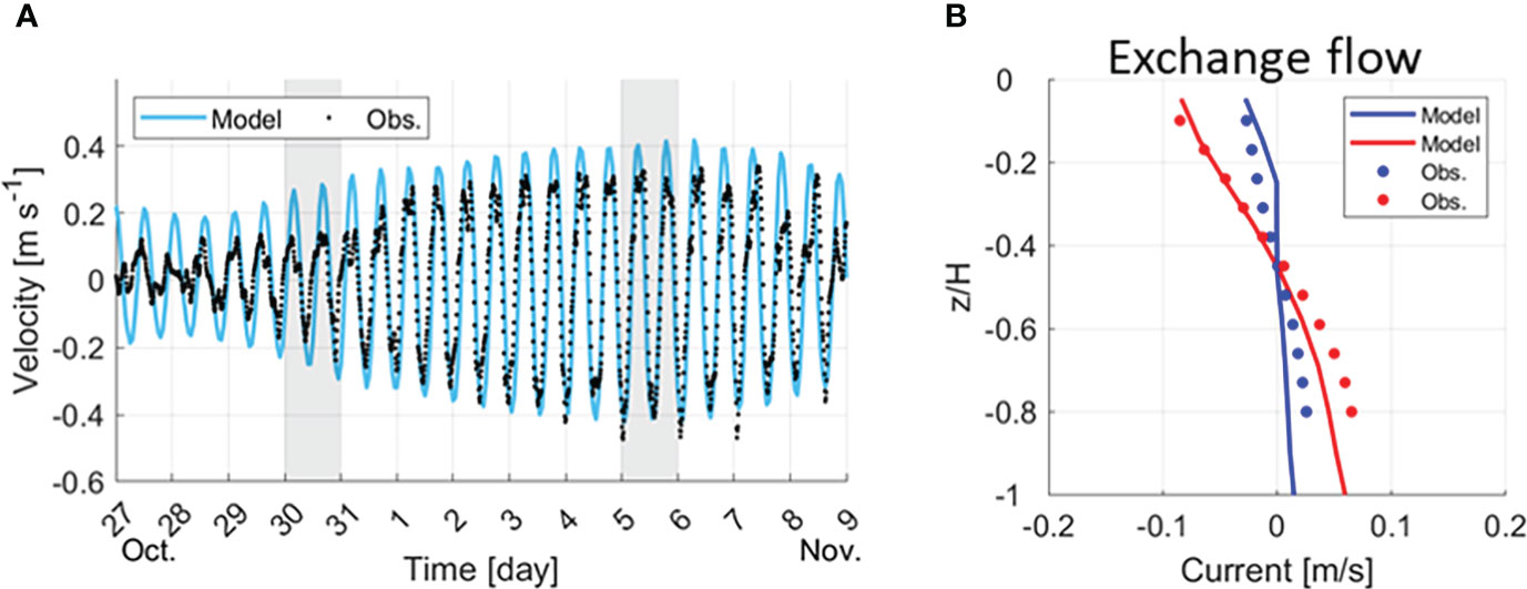
Figure 4 Comparison of flow rates between observations and the idealized model. (A) Time series of the depth-averaged velocity in observations (black dots) and the model (cyan line), with grey shading indicating Conductivity–Temperature–Depth (CTD) observation dates. (B) Vertical velocity profile of the observations (dots) and model (lines) during spring (red) and neap (blue) tides denoted by CTD observation data (grey shading boxes) in (A).

Decomposition of salt flux

The salinity distribution and the horizontal salinity gradient was estimated based on the salt flux. The along-channel salt flux was divided into seaward and landward fluxes (Fischer, 1972; Hunkins, 1981; MacCready, 2007). The driving mechanisms of the salt flux were examined by applying the flux decomposition method proposed by Lerczak et al. (2006).

The area-integrated, total along-channel salt flux was calculated as:

$\begin{array}{ll}F={\iint }^{}vsdA, & (2)\end{array}$

where the angled bracket denotes the tidal average; dA denotes the cross-sectional area of the individual grid cells estimated by multiplying dx and dz, where dx and dz are determined by the horizontal and vertical sizes of the individual grid cells in the cross-sectional areas. Note that dz is time-dependent owing to the changes in surface height, while v and s are the temporal along-channel velocity and salinity, respectively.

The cross-sectional area A at a particular along-channel location is divided into a constant number of differential element dA that constrict and expand with the tidal rise and fall of the free surface, respectively. The tidally averaged area (A₀) property is defined as follows:

$\begin{array}{ll}d{A}_0=dA, A_0={\iint }^{}dA,& (3)\end{array}$

where ʃʃ indicates the cross-sectional integral. Assessment of the contribution of the different processes to the salt fluxes requires decomposing the along-channel velocity and salinity fields into three components, which is the same as proposed by Lerczak et al. (2006): both tidally averaged over a tidal period and the area of cross-section component (v₀,s₀), tidally averaged and a cross-sectionally varying component (v_E, s_E), and tidally and cross-sectionally varying component (v_T,s_T):

$\begin{array}{ll}{v}_0=\frac{{\iint }^{}vdA}{A_0} & (4)\end{array}$

$\begin{array}{ll}{v}_E=\frac{vdA}{d{A}_0}-v_0 & (5)\end{array}$

$\begin{array}{ll}{v}_T=v-v_E-v_{0,}& (6)\end{array}$

There is a corresponding set of equations for the salinity. The variable v₀ is related to the river flow volume flux Q₀[=–v₀A₀, v_E is the estuarine exchange flow, and v_T represents tidal current. The tidal varying components v_T and s_T satisfy 〈v_TdA〉=0 and 〈s_TdA〉 =0 .Then, the total along-channel salt flux can be calculated as:

$$F={\iint }^{}\left(v_0+v_E+v_T\right)\left(s_0+s_E+s_T\right)dA$$

$$={\iint }^{}\left(v_0+v_E\right)\left(s_0+s_E\right)d{A}_0+{\iint }^{}\langle v_T{s}_{T}dA\rangle +cross terms$$

$\begin{array}{ll}=\underset{F_R}{\underbrace{-Q_0{S}_0}}+\underset{ F_E}{\underbrace{{\iint }^{}{v}_E{s}_{E}d{A}_0}}+\underset{F_T}{\underbrace{{\iint }^{}\langle v_T{s}_{T}dA\rangle }} & (7)\end{array}$

where the cross terms have been dropped because the results are negligible and uncorrelated by definition. Under this decomposition, F_R is the advective salt flux due to the river outflow, which is always a seaward salt flux; F_E is the salt flux resulting from steady shear dispersion, which is the spatial correlation of tidally averaged velocity and salinity; and F_T is the cross-sectionally integrated tidal oscillatory salt flux due to the correlation among tidal variations in velocity, salinity, and depth. Here, we use the low pass filter with 25 h to obtain the tidally averaged values.

Results and discussion

We primarily analyzed the results of the idealized model to exclude nonlinear effects caused by complex topography and focus on spring-neap variations. The realistic model results in 3.4 were referred to confirm that our main findings are applicable to the real estuary.

Periodic propagation of the horizontal salinity gradient

First, the spatiotemporal variability of the salinity distribution, which determines the horizontal salinity gradient, was investigated. In order to focus on the fortnightly variation of the salinity distribution, salinity at a 1-hour interval from the model was low pass filtered (25-hour) and sectionally averaged (Figure 5). The salinity distribution varied periodically (Figure 5B). During spring tides, the salt intrusion length was the shortest, the vertical salinity difference was less than 2, and it was vertically well-mixed (Figure 5C), and so the horizontal difference of salinity was large. During neap tides, the salt intrusion length was the longest and stratification was strong, and so the horizontal difference of salinity was small.

FIGURE 5

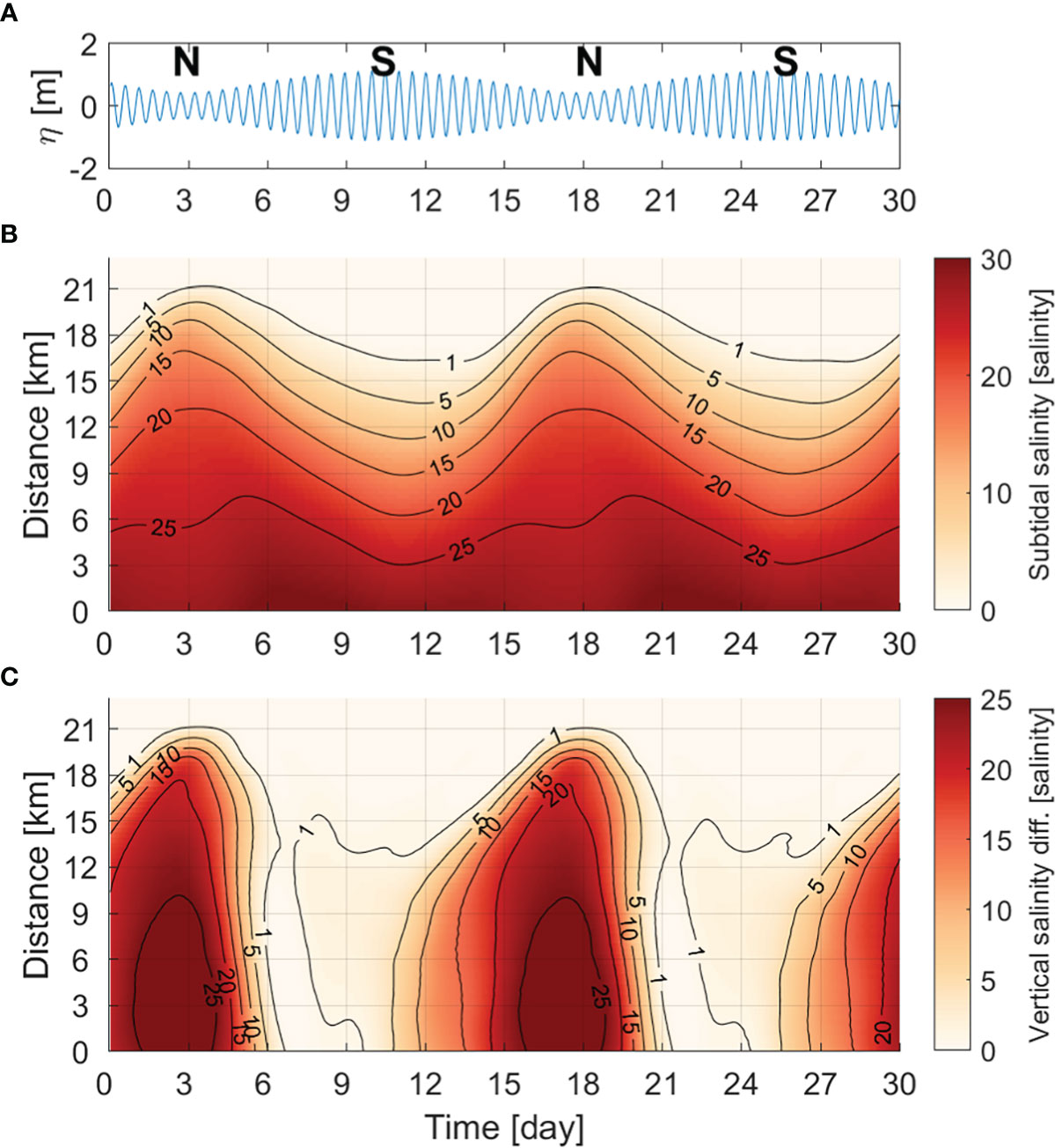
Figure 5 (A) Time series of sea-level height at the mouth of the idealized estuary and the N and S stand for neap tide and spring tide, respectively. Hovmöller diagram of (B) sectionally averaged subtidal salinity (unit: g kg^-1) and (C) the difference in salinity between the surface and bottom layer.

The variability of salt transport determines the variation of the length of the salt intrusion. Based on the commonly used subtidal salt flux decomposition for estuaries, the seaward salt flux due to river outflow is balanced by the landward salt flux due to the upstream dispersive mechanism (Ralston and Stacey, 2005; Lerczak et al., 2006; MacCready, 2007; Garcia et al., 2022). The composition of each salt flux was estimated using the decomposition method (Lerczak et al., 2006; MacCready, 2011; Chen et al., 2012). The total horizontal salt flux (F) exhibited marked fortnightly variability (Figure 6A). The fluctuation in F implies that the estuary gains salt when the tidal range decreases but loses salt when the tidal range increases. As the landward of the salt flux continues, the salt intrusion becomes longer, and as the seaward salt flux continues, the salt intrusion becomes shorter. Salt was imported by F_E and F_T, and F_E contributed approximately 80% of the total landward salt flux, on average, during the fortnightly tidal cycle (Figure 6B). The diffusive fraction of landward salt flux (v = F_T/(F_T+F_E)) after Hansen and Rattray (1966) was generally less than 0.5 when the total salt flux is landward. It also proves that the steady shear dispersion salt flux (F_E) is dominant in the landward salt flux.

FIGURE 6

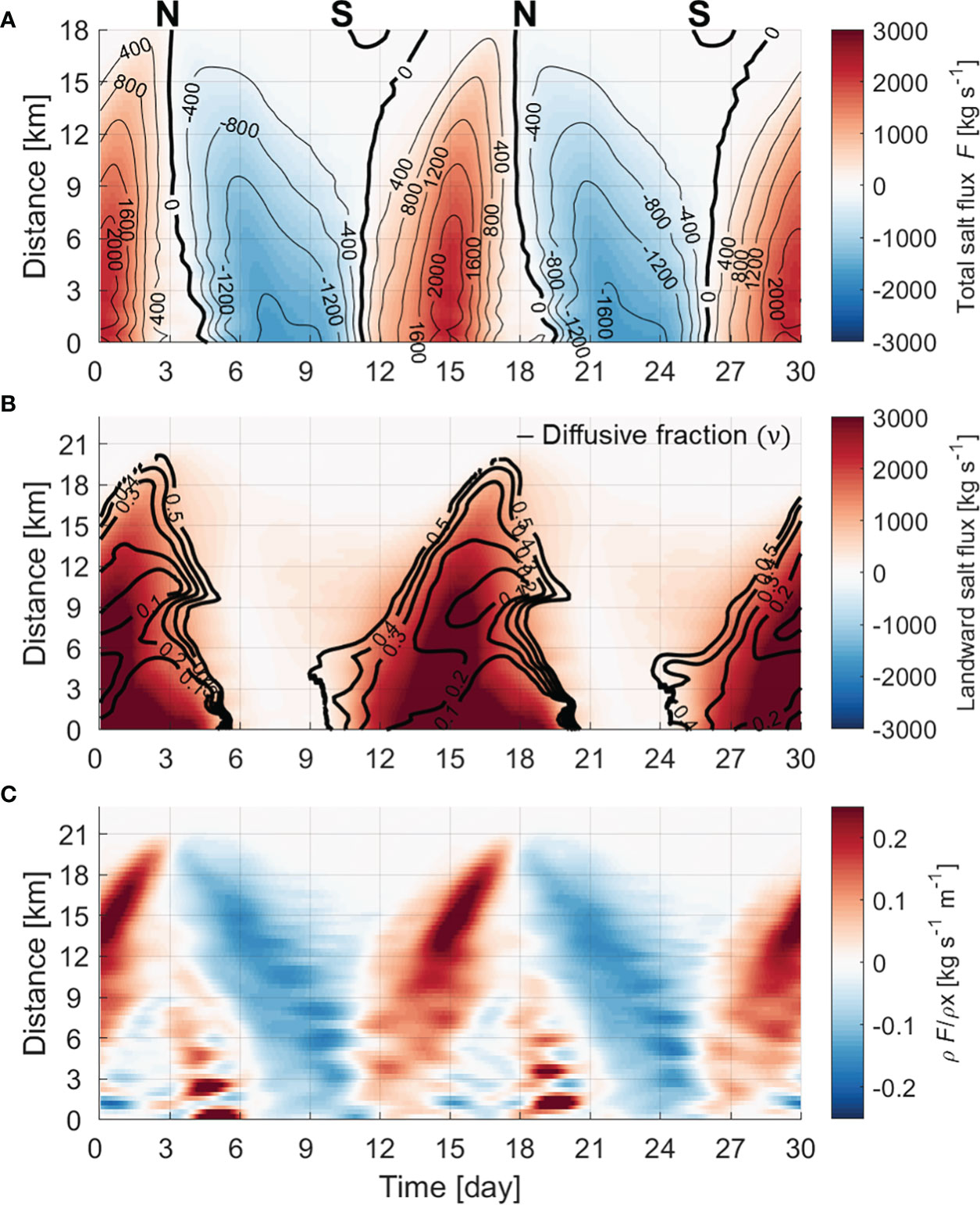
Figure 6 Hovmöller diagrams of the (A) total horizontal salt flux (F), (B) landward salt flux (color shading: steady shear dispersion salt flux [F_E] + tidal oscillatory salt flux [F_T]; unit: kgs^-1) and diffusive fraction (v; black contour lines), and (C) convergence of total salt flux (unit: kgs^-1m^-1).

The horizontal salinity gradient along the channel also exhibited distinct fortnightly variation (Figure 7A). During spring tides, the salinity gradient was relatively high from the mouth and was the highest (> 2.0km^-1) around the middle estuary (~10 km from the mouth). While the tidal range was decreasing, the maximum salinity gradient propagated to the head of estuary, becoming larger and reaching at least 5.0 km^-1 during neap tides. Then, while the tidal range increased, the maximum salinity gradient retreated from the head. Thus, the fortnightly variation of the maximum salinity gradient was out of phase between the lower and upper estuary (Figure 7B). The time-varying maximum salinity gradient is similar to the results from the Hudson River estuary (Ralston et al., 2008; Geyer and Ralston, 2015). However, the maximum salinity gradient was maintained at the head without changing the position until the next spring tide in the Hudson River estuary, which differs from the Sumjin River estuary. Owing to its long length, the salinity distribution in the Hudson River estuary cannot immediately respond to the tidal cycle in the upper estuary (Park and Kuo, 1996; Lerczak et al., 2009). Therefore, the maximum salinity gradient in the upper estuary may persist.

FIGURE 7

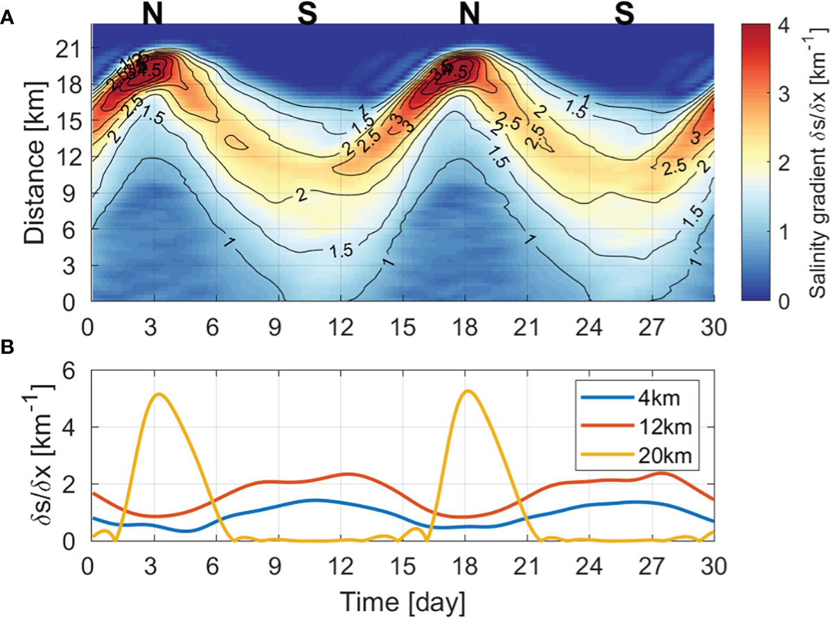
Figure 7 Hovmöller diagram of (A) horizontal salinity gradient along the channel (unit: km^-1) and (B) time series of salinity gradient at 4, 12, and 20 km.

In the estuary considered in this study, the continuous movement of a high salinity gradient along channel is related to the convergence of the salt flux, (∂F/∂x) The stronger the convergence becomes, the greater the horizontal difference in salinity and a salinity gradient occurs. As the convergence decreases, the horizontal difference in salinity decreases. That is, the movement of the maximum salinity gradient zone can be determined by the convergence of the salt flux. Figure 6C shows the spatiotemporal change of the convergence of the salt flux. When the total salt flux is landward (seaward), the greater the positive (negative) value, the stronger the convergence. While the tidal range decreases after a spring tide, salt is imported into the estuary owing to the steady shear dispersion salt flux. As the salt intrusion length becomes longer, the high salinity gradient propagates toward the head of the estuary. The convergence of the salt flux also becomes stronger as it moves toward the estuary head, especially from 12 km to the head. Therefore, the salinity gradient increases from 2 to 6 km^-1 from the middle estuary to the head. While the tidal range increases after the neap tide, salt is exported out of the estuary owing to the advective salt flux, and as the salt intrusion length is shortened, the salinity gradient also moves toward the mouth. Owing to constant convergence in the seaward direction, a salinity gradient of 2 km^-1 or more moves toward the mouth. As such, the salinity gradients in the lower and upper estuary have different time changes (Figure 7B), which has a major effect on the exchange flow.

Fortnightly variation in exchange flow and its cause

To analyze the fortnightly variation of exchange flow in the entire estuary, we calculated the intensity of exchange flow by averaging the absolute values with depth (Burchard et al., 2011). If the intensity is 0.04 or more (unit: ms^-1), the exchange flow can be set as strong, because at this intensity, F_E due to the exchange flow can induce the total salt flux landward. Uniquely, the exchange flow was strong (> 0.04 ms^-1) in the lower and middle estuary around the spring tide and was generally weak during increasing tidal range, but strong during decreasing tidal range (Figure 8A). Therefore, there was a phase difference depending on the location (Figure 8B). In the lower estuary, it was at a maximum around the spring tide and a minimum after 2–3 days of the peak neap tide. In the upper estuary, it was strongest before and after the neap tide and weakest during the spring tide.

FIGURE 8

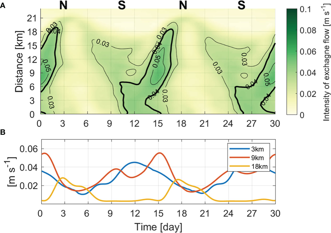
Figure 8 (A) Hovmöller diagram of the depth-averaged absolute value of the exchange flow and (B) timeseries of the intensity of the exchange flow at 3, 9, and 18 km from the estuary mouth (unit: ms^-1).

In a previous study of the Sumjin River estuary, the salinity gradient was the main determinant in the fortnightly variation of exchange flow in the lower estuary (Cho et al., 2020). To determine what mechanism caused the variation in the intensity of the exchange flow in the entire estuary, we compared the salinity gradient and vertical mixing effect, which are the main factors that determine the vertical shear of the exchange flow. The horizontal Richardson number (Ri_x), also referred as the Simpson number, has been used to provide a diagnostic balance between baroclinic forcing and vertical mixing due to tidal friction (Stanev et al., 2015; Li et al., 2018). We calculated Ri_x according to previous studies (MacCready and Geyer, 2010; Rayson et al., 2017) to identify the main factor that determines the exchange flow:

$\begin{array}{ll}R{i}_x=\frac{g\beta H^2\left(\partial s/\partial x\right)}{C_d{u}_b{}^2},& (8)\end{array}$

where β is the saline contraction coefficient of 7.7 ×10^-4 proposed by Wang et al. (2015), g is the acceleration due to gravity, ∂s/∂x is the horizontal salinity gradient, H is the local water depth, C_d(4.0 ×10⁻³ ) is the drag coefficient (used in the model setting), and u_b is the amplitude of the bottom tidal velocity (Stacey et al., 2001). There is considerable variation in the estimate of the critical value for Ri_x (MacCready and Geyer, 2010); it is less than 1 or set to 3 (Stacey et al., 2001; MacCready and Geyer, 2010; Li et al., 2018). Since we use the bottom tidal velocity, vertical mixing is weaker than when using the depth-mean tidal velocity (Pein et al., 2014; Schulz et al., 2015; Stanev et al., 2015; Li et al., 2018) and the salinity gradient is large; therefore, the Ri_x is generally higher than 1. As such, we set the critical value to 3 in order to identify the main factor that strengthens the vertical shear of the exchange flow.

The baroclinic forcing and vertical mixing, which determine Ri_x, differ in the timing and location of their strong appearance (Figures 9A, B). Between lower and upper estuaries, baroclinic forcing has out-of-phase variability but vertical mixing exhibits relatively in-phase variability. According to Eq. (8), baroclinic forcing is mainly determined by the horizontal salinity gradient. Therefore, the subtidal variation in baroclinic forcing was nearly consistent with the horizontal salinity gradient (Figure 7A). During tidal range decreases, the exchange flow became stronger toward the head of the estuary because vertical mixing gradually decreased, but the baroclinic forcing effect became predominant as the maximum salinity gradient moved to the head (Ri_x>3 > 3; Figure 9C). After the neap tide, as the tidal range increased, vertical mixing became stronger throughout the estuary, the baroclinic forcing effect became insignificant (Ri_x ≈ 1) , and the vertical shear of exchange flow weakened. The spatiotemporal changes with high Ri_x (> 3) and strong exchange flow (> 0.04 m s^-1) agree relatively well. Therefore, the determinant of the fortnightly variation of exchange flow not only in the lower estuary but also in the entire estuary is the salinity gradient, and the phase difference occurs in the lower and upper estuaries because the salinity gradient is out of phase between lower and upper estuaries.

FIGURE 9

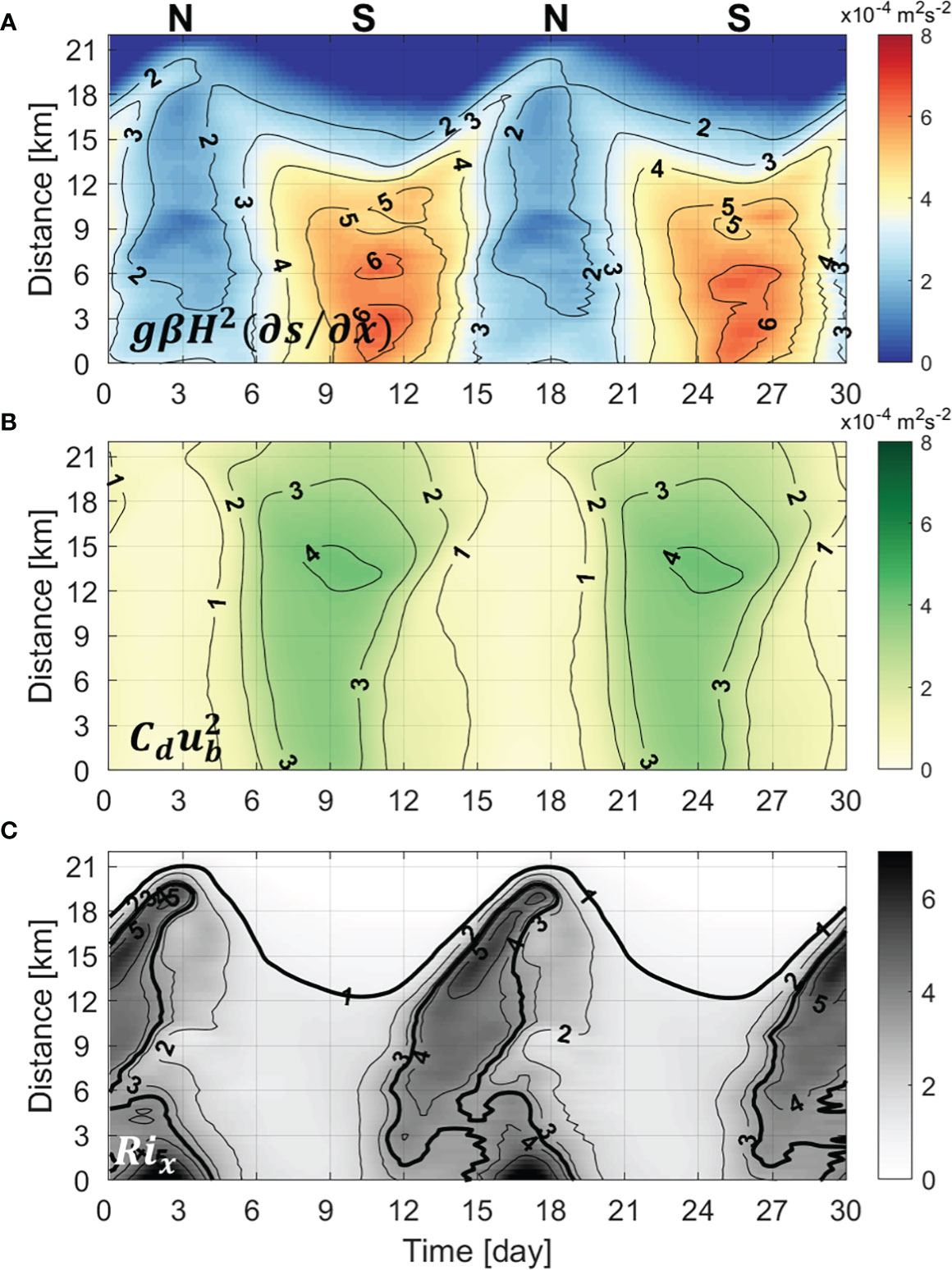
Figure 9 Hovmöller diagram of the (A) baroclinic forcing (unit: × 10⁴ m² s^-2), (B) bottom stress (unit: × 10⁴ m² s^-2), and (C) nondimensional horizontal Richardson number.

Restriction of salt intrusion by vertical mixing

Unlike many estuaries, in the Sumjin River estuary, the exchange was stronger during spring tide than during neap tide in the lower estuary. This was also confirmed through the idealized model experiment, and it was quantitatively proved with Ri_x that the salinity gradient effect was large enough to overwhelm the vertical mixing effect. In order for the salinity gradient to be sufficiently large during the spring tide, the response time of salinity distribution must coincide with the timescale of variation in vertical mixing (Park and Kuo, 1996). As vertical mixing increases, the salinity gradient increases, which can be the maximum during spring tides. In particular, this phenomenon occurs in short estuaries rather than long estuaries where the timescale of mass response is long (Park and Kuo, 1996). We estimated the vertical eddy diffusivity of salt (K_s) to examine the intensity of vertical mixing, which is the most common approach for quantification of the mixing in estuaries (Fischer, 1972; MacCready, 2007). We selected the 5 g kg^-1 isohaline of bottom salinity to represent the salt intrusion length (Figure 10). A scatter plot of the salt intrusion distinctly shows an inverse linear relationship between the isohaline length and K_s. During the spring tide, when vertical mixing was strongest, the salinity gradient was at its maximum because the salt intrusion was at its minimum.

FIGURE 10

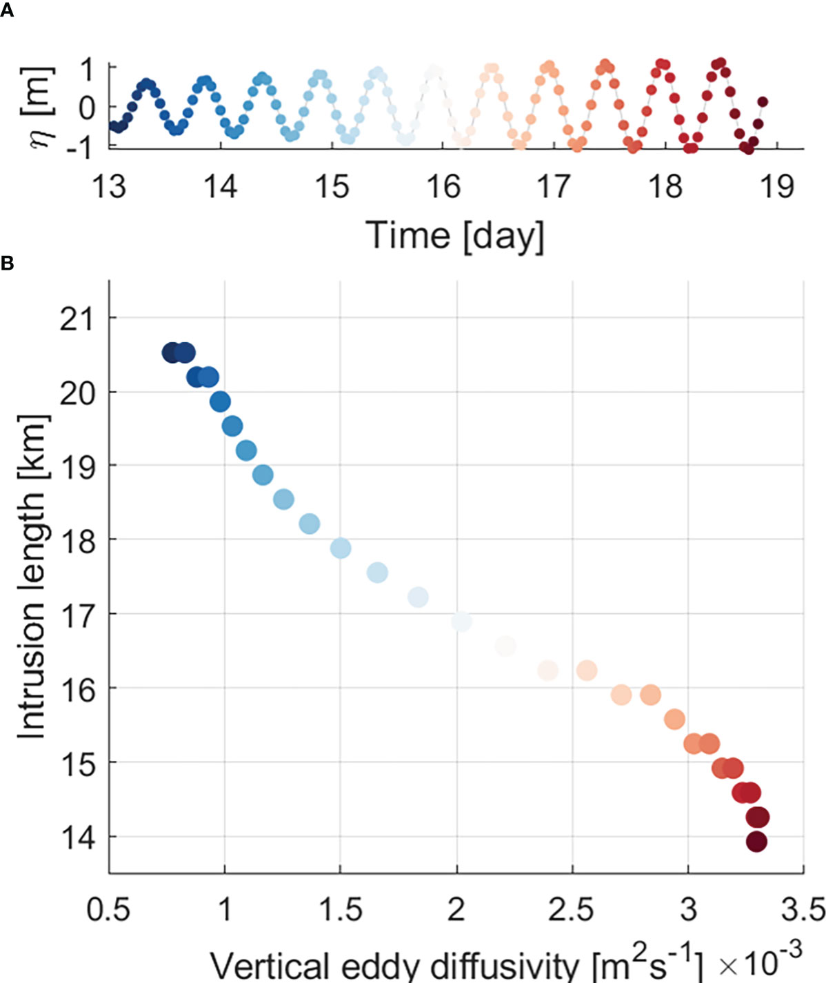
Figure 10 (A) Time series of sea-surface height (unit: m) and (B) scatter plot of intrusion length (unit: km) of the 5 gkg^-1 isohaline versus cross-sectionally averaged vertical eddy diffusivity K_s (unit: m² s^-1) from the model results. Each colored dot in (B) indicates each timing denoted by the same colored dot in (A).

The relationship between exchange flow and salinity gradient with respect to vertical mixing can be summarized as follows. As vertical mixing increases, the vertical shear of exchange flow decreases and stratification weakens. As a result, F_E driving the landward salt flux decreases, and the total salt flux becomes seaward, resulting in salt intrusion that is shortened but vertically homogenous. During the spring tide, salt intrusion is minimal, and the salinity gradient in the lower estuary is large (~ 2.3 km^-1); we found that it was 2–4 times larger than that of other longer estuaries (e.g., 1 km^-1 in the Modaomen estuary [~ 63 km] and 0.6 km^-1 in the Hudson River estuary [> 100 km]). The salinity gradient was large enough to overwhelm the vertical mixing effect, which intensifies the vertical shear of exchange flow, resulting in the development of stratification. Therefore, as F_E increases, the total salt flux becomes landward. As the tidal range decreases, salt is imported into the estuary and salt intrusion becomes longer. The strengthening of the convergence of the landward salt flux during this period induces the maximum salinity gradient to proceed further into the estuary. This process is repeated while the tidal range decreases, such that the maximum salinity gradient at the head enhances the exchange flow during the neap tide.

Model application to realistic topography in the Sumjin River estuary

The idealized model clearly showed the variations of salinity gradient in the entire short estuary and its effect on the exchange flow over fortnightly tidal cycles. However, the idealized model did not consider the effect of complicated topography on variations in the salinity gradient and exchange flow. A numerical experiment with realistic topography was conducted to confirm the spatiotemporal variations of the salinity gradient and exchange flow in the Sumjin River estuary. For the realistic model, the river discharge rate (30 m³s^-1) in 2013 was applied. Other model settings were the same as those used in the idealized model experiment.

The realistic model appropriately simulated the fortnightly variation in the depth-averaged salinity and the horizontal salinity gradient (Figures 3E–J). The horizontal salinity gradient changed periodically over fortnightly tidal cycles as in the idealized model experiment, although its large value appeared sparsely owing to an uneven depth distribution (Figure 11). Occurrence of large horizontal salinity gradients may be attributed to the saline waters which persist for a few days due to irregular depth. The spatiotemporal change of exchange flow corresponds well with that of the horizontal salinity gradient, which shows out of phase between lower and upper estuaries, as in the idealized model experiment.

FIGURE 11

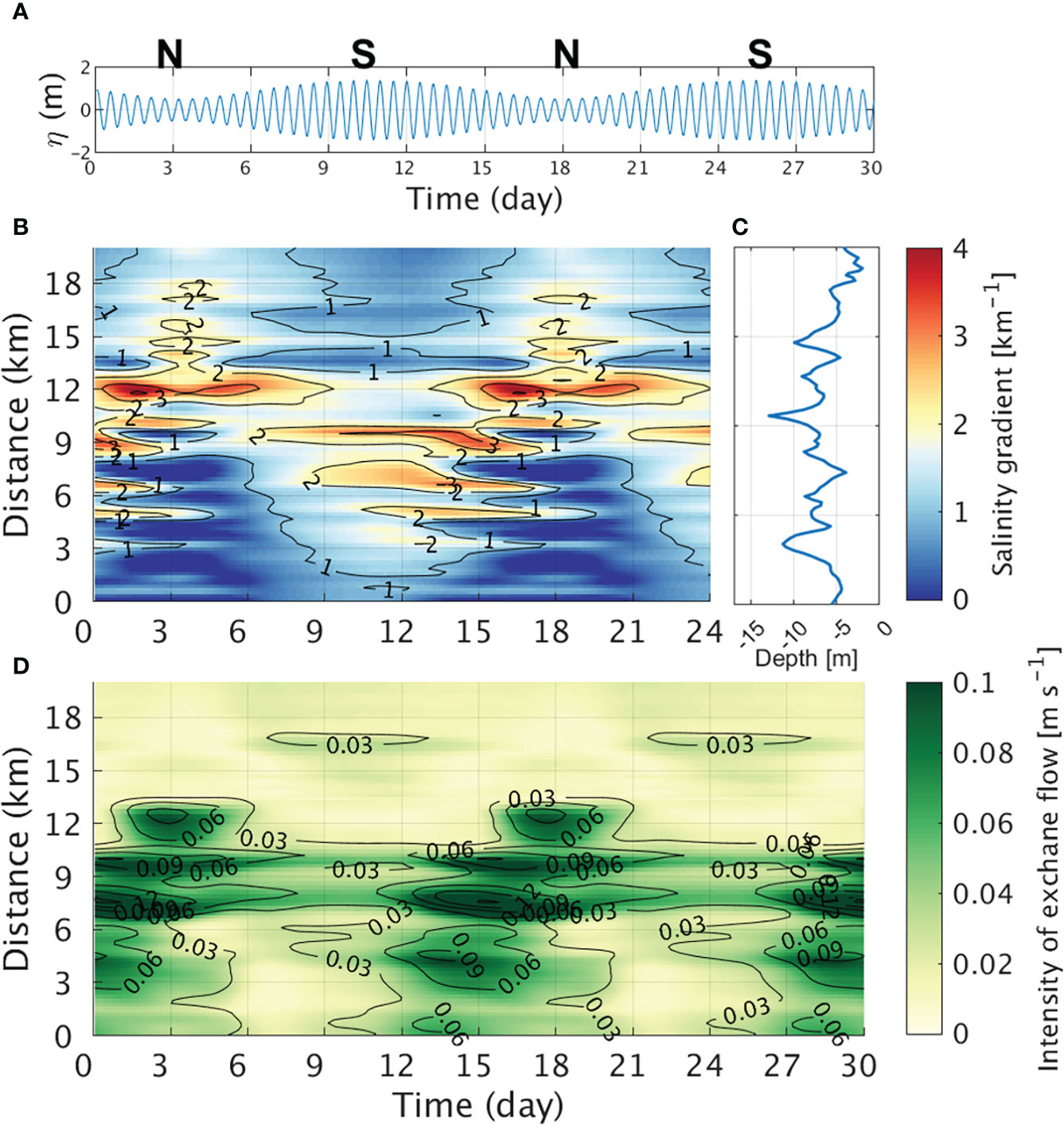
Figure 11 (A) Time series of sea-level height at the mouth of the real case and the N and S stand for neap tide and spring tide, respectively. Hovmöller diagram of (B) horizontal salinity gradient along the channel (unit: km^-1). (C) Depth variation in the Sumjin River estuary toward upstream, which is averaged across the channel (unit: m). (D) Hovmöller diagram of the depth-averaged absolute value of the exchange flow (unit: ms^-1).

Both idealized and realistic models showed the larger salinity gradient and the stronger exchange flow variation during the spring tide, which is consistent with the observations of Cho et al. (2020) in the lower estuary. However, the model results suggest that the salinity gradient is smaller and the exchange flow is weaker in the upper estuary during the spring tide, but it is opposite to that in the lower estuary.

Summary and conclusions

Fortnightly variation of horizontal salinity gradient and exchange flow, and their mechanism, were investigated in an estuary with a short length and narrow width (i.e., the Sumjin River estuary). The fortnightly variation of the exchange flow had a different phase in the lower and upper estuary: in the lower estuary, it was strong during spring tides, but in the upper estuary, it was strong during neap tides.

During transitions from spring to neap tides, vertical mixing becomes weaker and baroclinic forcing dominates owing to the maximum salinity gradient moving from the mouth to the head. This intensifies the vertical shear of exchange flow and develops stratification, increasing the steady shear dispersion salt flux. Therefore, the total salt flux is landward and the salt intrusion becomes longer. Where convergence is strong while the salt flux is landward, the salinity gradient is at a maximum, making the exchange flow stronger toward the inside of the estuary. The salt intrusion continues to lengthen, and the salinity gradient at the head of estuary is maximized and the exchange flow is also strong during neap tides. While the tidal range increases, vertical mixing becomes stronger throughout the estuary and more dominant than the baroclinic forcing effect, resulting in weaker exchange flow and decreased landward salt flux. The total salt flux is seaward by the advective salt flux. As salt is exported out of the estuary, salt intrusion continues to be shortened. Owing to the minimum salt intrusion during the spring tide, the salinity gradient increases in the lower estuary.

As vertical mixing decreases after the peak spring tide, baroclinic forcing becomes dominant, and the exchange flow begins to intensify again. The determinant of the fortnightly variation of exchange flow in the entire estuary is the salinity gradient. The spatiotemporal change of strong exchange flow (> 0.04 m s^-1) corresponds well with that of high Simpson number (Ri_x > 3). Owing to the change in the salt intrusion determined by vertical mixing, the maximum salinity gradient periodically reciprocates, while the tidal range decreases; this dominates the vertical mixing effect, enhancing the exchange flow. Since the maximum salinity gradient is out of phase between the lower and upper estuaries, the phase of the exchange flow also varies depending on the location of the estuary.

Fortnightly variation in the salinity gradient and exchange flow also appeared in the model using realistic topography for the Sumjin River estuary although the non-linear topographic effects disturbed the fortnightly oscillation of the maximum salinity gradient zone and the exchange flow. This study proposes that the observations at a specific point cannot represent the fortnightly variation in the horizontal salinity gradient and exchange flow. The spatiotemporal variation over the entire estuary should be investigated to understand the estuarine circulation in a short and narrow estuary like the Sumjin River estuary.

Data availability statement

The raw data supporting the conclusions of this article will be made available by the authors, without undue reservation.

Author contributions

Conceptualization, E-BC and Y-KC. Methodology, E-BC and Y-KC. writing draft, E-BC. review and editing, Y-KC, Y-JT, and HN. visualization, E-BC. supervision, Y-KC and Y-JT. All authors contributed to the article and approved the submitted version.

Funding

This research was supported by the Korea Institute of Marine Science & Technology Promotion(KIMST) funded by the Ministry of Oceans and Fisheries (20220541) and the National Research Foundation (NRF) funded by the Korean government (NRF-2022M3I6A1085573).

Conflict of interest

The authors declare that the research was conducted in the absence of any commercial or financial relationships that could be construed as a potential conflict of interest.

Publisher’s note

All claims expressed in this article are solely those of the authors and do not necessarily represent those of their affiliated organizations, or those of the publisher, the editors and the reviewers. Any product that may be evaluated in this article, or claim that may be made by its manufacturer, is not guaranteed or endorsed by the publisher.

References

Andutta F. P., de Miranda L. B., Franca Schettini C. A., Siegle E., da Silva M. P., Izumi V. M., et al. (2013). Temporal variations of temperature, salinity and circulation in the peruipe river estuary (nova vicosa, ba). Contin. Shelf Res. 70, 36–45. doi: 10.1016/j.csr.2013.03.013

CrossRef Full Text | Google Scholar

Becker M. L., Luettich R. A., Seim H. (2009). Effects of intratidal and tidal range variability on circulation and salinity structure in the cape fear river estuary, north carolina. J. Geophys. Res. 114, (C4). doi: 10.1029/2008JC004972

CrossRef Full Text | Google Scholar

Bowen M. M., Geyer W. R. (2003). Salt transport and the time-dependent salt balance of a partially stratified estuary. J. Geophys. Res. Oceans 108, (C5). doi: 10.1029/2001JC001231

CrossRef Full Text | Google Scholar

Burchard H., Hetland R. D., Schulz E., Schuttelaars H. M. (2011). Drivers of residual estuarine circulation in tidally energetic estuaries: Straight and irrotational channels with parabolic cross section. J. Phys. Oceanogr. 41, 548–570. doi: 10.1175/2010JPO4453.1

CrossRef Full Text | Google Scholar

Chen S.-N., Geyer W. R., Ralston D. K., Lerczak J. A. (2012). Estuarine exchange flow quantified with isohaline coordinates: Contrasting long and short estuaries. J. Phys. Oceanogr. 42, 748–763. doi: 10.1175/JPO-D-11-086.1

CrossRef Full Text | Google Scholar

Cho E.-B., Cho Y.-K., Kim J. (2020). Enhanced exchange flow during spring tide and its cause in the sumjin river estuary, korea. Estuaries Coasts. 43, 525–534. doi: 10.1007/s12237-019-00636-9

CrossRef Full Text | Google Scholar

de Miranda L. B., Bérgamo A. L., de Castro B. M. (2005). Interactions of river discharge and tidal modulation in a tropical estuary, ne brazil. Ocean Dyn. 55, 430–440. doi: 10.1007/s10236-005-0028-z

CrossRef Full Text | Google Scholar

Dijkstra Y. M., Schuttelaars H. M., Burchard H. (2017). Generation of exchange flows in estuaries by tidal and gravitational eddy viscosity-shear covariance (esco). J. Geophys. Res. Oceans. 122, 4217–4237. doi: 10.1002/2016JC012379

CrossRef Full Text | Google Scholar

Fischer H. (1972). Mass transport mechanisms in partially stratified estuaries. J. Fluid Mech. 53, 671–687. doi: 10.1017/S0022112072000412

CrossRef Full Text | Google Scholar

Garcia A. M. P., Geyer W. R., Randall N. J. E. (2022). Exchange flows in tributary creeks enhance dispersion by tidal trapping. Estuaries Coasts. 45, 363–381. doi: 10.1007/s12237-021-00969-4

CrossRef Full Text | Google Scholar

Garel E., Ferreira Ó. (2013). Fortnightly changes in water transport direction across the mouth of a narrow estuary. Estuaries Coasts. 36, 286–299. doi: 10.1007/s12237-012-9566-z

CrossRef Full Text | Google Scholar

Geyer W. R., MacCready P. (2014). The estuarine circulation. Annu. Rev. Fluid Mech. 46, 175–197. doi: 10.1146/annurev-fluid-010313-141302

CrossRef Full Text | Google Scholar

Geyer W. R., Ralston D. K. (2015). Estuarine frontogenesis. J. Phys. Oceanogr. 45, 546–561. doi: 10.1175/JPO-D-14-0082.1

CrossRef Full Text | Google Scholar

Geyer W. R., Trowbridge J. H., Bowen M. M. (2000). The dynamics of a partially mixed estuary. J. Phys. Oceanogr. 30, 2035–2048. doi: 10.1175/1520-0485(2000)030<2035:TDOAPM>2.0.CO;2

CrossRef Full Text | Google Scholar

Gong W. P., Maa J. P.-Y., Hong B., Shen J. (2014). Salt transport during a dry season in the modaomen estuary, pearl river delta, china. Ocean Coast. Management. 100, 139–150. doi: 10.1016/j.ocecoaman.2014.03.024

CrossRef Full Text | Google Scholar

Hansen D. V., Rattray J. M. (1966). New dimensions in estuary classification 1. Limnology Oceanography. 11 (3), 319–326. doi: 10.4319/lo.1966.11.3.0319

CrossRef Full Text | Google Scholar

Hunkins K. (1981). Salt dispersion in the hudson estuary. J. Phys. Oceanogr. 11, 729–738. doi: 10.1175/1520-0485(1981)011<0729:SDITHE>2.0.CO;2

CrossRef Full Text | Google Scholar

Large W. G., McWilliams J. C., Doney S. C. (1994). Oceanic vertical mixing: A review and a model with a nonlocal boundary layer parameterization. Rev. Geophys. 32, 363–403. doi: 10.1029/94RG01872

CrossRef Full Text | Google Scholar

Lerczak J. A., Geyer W. R., Chant R. J. (2006). Mechanisms driving the time-dependent salt flux in a partially stratified estuary. J. Phys. Oceanogr. 36, 2296–2311. doi: 10.1175/JPO2959.1

CrossRef Full Text | Google Scholar

Lerczak J. A., Geyer W. R., Ralston D. K. (2009). The temporal response of the length of a partially stratified estuary to changes in river flow and tidal amplitude. J. Phys. Oceanogr. 39 (4), 915–933. doi: 10.1175/2008jpo3933.1

PubMed Abstract | CrossRef Full Text | Google Scholar

Li X., Geyer W. R., Zhu J., Wu H. (2018). The transformation of salinity variance: A new approach to quantifying the influence of straining and mixing on estuarine stratification. J. Phys. Oceanogr. 48, 607–623. doi: 10.1175/JPO-D-17-0189.1

CrossRef Full Text | Google Scholar

Li C., O’Donnell J. (2005). The effect of channel length on the residual circulation in tidally dominated channels. J. Phys. Oceanogr. 35, 1826–1840. doi: 10.1175/JPO2804.1

CrossRef Full Text | Google Scholar

MacCready P. (2007). Estuarine adjustment. J. Phys. Oceanogr. 37, 2133–2145. doi: 10.1175/JPO3082.1

CrossRef Full Text | Google Scholar

MacCready P. (2011). Calculating estuarine exchange flow using isohaline coordinates. J. Phys. Oceanogr. 41, 1116–1124. doi: 10.1175/2011JPO4517.1

CrossRef Full Text | Google Scholar

MacCready P., Geyer W. R. (2010). Advances in estuarine physics. Annu. Rev. Mar. Sci. 2, 35–58. doi: 10.1146/annurev-marine-120308-081015

CrossRef Full Text | Google Scholar

Mantovanelli A., Marone E., da Silva E. T., Lautert L. F., Klingenfuss M. S., Prata V. P., et al. (2004). Combined tidal velocity and duration asymmetries as a determinant of water transport and residual flow in paranagua bay estuary. Estuar. Coast. Shelf Sci. 59, 523–537. doi: 10.1016/j.ecss.2003.09.001

CrossRef Full Text | Google Scholar

Park K., Kuo A. Y. (1996). Effect of variation in vertical mixing on residual circulation in narrow, weakly nonlinear estuaries. Coast. Estuar. Stud. 53, 301–317. doi: 10.1029/CE053p0301

CrossRef Full Text | Google Scholar

Pein J. U., Stanev E. V., Zhang Y. J. (2014). The tidal asymmetries and residual flows in ems estuary. Ocean Dyn. 64, 1719–1741. doi: 10.1007/s10236-014-0772-z

CrossRef Full Text | Google Scholar

Pritchard D. W. (1967). What Is an Estuary: Physical Viewpoint (Washington. D.C: American Association for the Advancement of Science, Washington Publications).

Google Scholar

Ralston D. K., Geyer W. R., Lerczak J. A. (2008). Subtidal salinity and velocity in the hudson river estuary: Observations and modeling. J. Phys. Oceanogr. 38, 753–770. doi: 10.1175/2007JPO3808.1

CrossRef Full Text | Google Scholar

Ralston D. K., Stacey M. T. (2005). Longitudinal dispersion and lateral circulation in the intertidal zone. J. Geophys. Res. Oceans 110, (C7). doi: 10.1029/2005JC002888

CrossRef Full Text | Google Scholar

Rayson M. D., Gross E. S., Hetland R. D., Fringer O. B. (2017). Using an isohaline flux analysis to predict the salt content in an unsteady estuary. J. Phys. Oceanogr. 47, 2811–2828. doi: 10.1175/JPO-D-16-0134.1

CrossRef Full Text | Google Scholar

Schulz E., Schuttelaars H. M., Gräwe U., Burchard H. (2015). Impact of the depth-to-width ratio of periodically stratified tidal channels on the estuarine circulation. J. Phys. Oceanogr. 45, 2048–2069. doi: 10.1175/JPO-D-14-0084.1

CrossRef Full Text | Google Scholar

Scully M. E., Geyer W. R., Lerczak J. A. (2009). The influence of lateral advection on the residual estuarine circulation: A numerical modeling study of the hudson river estuary. J. Phys. Oceanogr. 39, 107–124. doi: 10.1175/2008JPO3952.1

CrossRef Full Text | Google Scholar

Shaha D. C., Cho Y.-K. (2009). Comparison of empirical models with intensively observed data for prediction of salt intrusion in the sumjin river estuary, korea. Hydrol. Earth Syst. Sci. 13, 923–933. doi: 10.5194/hess-13-923-2009

CrossRef Full Text | Google Scholar

Shchepetkin A. F., McWilliams J. C. (2005). The regional oceanic modeling system (roms): A split-explicit, free-surface, topography-following-coordinate oceanic model. Ocean Modell. 9, 347–404. doi: 10.1016/j.ocemod.2004.08.002

CrossRef Full Text | Google Scholar

Stacey M. T., Burau J. R., Monismith S. G. (2001). Creation of residual flows in a partially stratified estuary. J. Geophys. Res. 106, 17013–17037. doi: 10.1029/2000JC000576

CrossRef Full Text | Google Scholar

Stanev E. V., Al-Nadhairi R., Valle-Levinson A. (2015). The role of density gradients on tidal asymmetries in the German bight. Ocean Dyn. 65, 77–92. doi: 10.1007/s10236-014-0784-8

CrossRef Full Text | Google Scholar

Uncles R. J., Stephens J. A. (1990). The structure of vertical current profiles in a macrotidal, partly-mixed estuary. Estuaries. 13, 349–361. doi: 10.2307/1351780

CrossRef Full Text | Google Scholar

Valle-Levinson A. (2010). Contemporary issues in estuarine physics (Cambridge, UK: Cambridge University Press).

Google Scholar

Wang T., Geyer W. R., Engel P., Jiang W. S., Feng S. Z. (2015). Mechanisms of tidal oscillatory salt transport in a partially stratified estuary. J. Phys. Oceanogr. 45 (11), 2773–2789. doi: 10.1175/jpo-d-15-0031.1

CrossRef Full Text | Google Scholar

Wei X., Williams M. E., Brown J. M., Thorne P. D., Amoudry L. O. (2022). Salt intrusion as a function of estuary length in periodically weakly stratified estuaries. Geophys. Res. Lett. 49 (15). doi: 10.1029/2022GL099082

CrossRef Full Text | Google Scholar