 Fangjie Yu
 Fengzhi Sun
 Jianchao Li
 Ge Chen
- 1College of Information Science and Engineering, Ocean University of China, Qingdao, China
- 2Laboratory for Regional Oceanography and Numerical Modeling, Qingdao National Laboratory for Marine Science and Technology, Qingdao, China
- 3Key Laboratory of Mariculture, Ministry of Education, Ocean University of China, Qingdao, China
The South Yellow Sea Cold Water Mass (SYSCWM), which occurs in the South Yellow Sea (SYS) during summer, significantly impacts the hydrological characteristics and marine ecosystems but lacks fine interior data. With satellite observations, significant achievements have been made in reconstructing high-resolution ocean subsurface thermohaline structure based on machine learning. However, the accuracy of offshore subsurface parameter estimation will be affected due to the macro-tidal environment and fewer in situ observations. In this paper, we coupled the TPXO tide model and Light Gradient Boosting Machine algorithm to develop an inversion model of offshore subsurface thermal structure for the SYS using sea surface data and in situ observations. After light modelling, the subsurface temperature structure in the SYS is retrieved from sea surface parameters with a spatial resolution of 0.25° at depths of 0-55 m. Observation-based dataset (ARMOR3D) and in situ observations are used for model evaluation. According to the validation of the mooring buoy observations, the overall coefficient of determination (R2), which determines the percentage of variance in the dependent variable that can be explained by the independent variable, is more than 0.95. Furthermore, the R2 is improved by 12% due to coupling tide model below the thermocline during the maturity stage of SYSCWM, which is helpful for a better reconstruction of SYSCWM. Comparing with the cruise data, the average R2 of the proposed model is 0.927 which is slightly better than the accuracy of the observation-based ARMOR3D dataset. Since the R2 exceeds 0.8 in the most area of 121°E~123.5°E, 33°N~36°N, the reconstruction is reliable in this area. The method provides a new explorable direction for reconstructing the ocean thermal structure in offshore areas.
1. Introduction
The South Yellow Sea (SYS) is a shallow (average depth of 46 m), semi-enclosed marginal sea in the northwestern Pacific between the Chinese mainland and the Korean Peninsula. Due to the vast and shallow continental shelf, seasonally atmospheric conditions, such as the Asian monsoon, significantly impact the thermal structure of SYS (Chu et al., 1997; Sun et al., 2022). In the winter, strong northwest winds drive the water column to be well-mixed until spring. Weak southeasterly winds prevail in summer, so enhanced solar radiation causes the rapid formation of a strong and stable seasonal thermocline, preventing vertical mixing between the upper mixed layer and deep layer so that the cold water from the previous winter is reserved below the thermocline (Lee et al., 2016). It is called the South Yellow Sea Cold Water Mass (SYSCWM; Li et al., 2017a) in the SYS, which occupies the bottom layers of the central part with a large temperature difference between the surface and the bottom. The SYSCWM plays an important role in the field of hydrodynamics and biochemistry (Wang et al., 2014; Liu et al., 2015; Xin et al., 2015; Li et al., 2016; Guo et al., 2021; Li et al., 2021). The Yellow Sea Warm Current in winter is another prominent feature in the SYS, which transports warm saline water from the Tsushima Warm Current to the SYS (Zhang et al., 2008; Diao et al., 2022; Yu et al., 2022). In addition, SYS is a macro-tidal environment with a huge tidal range and strong tidal currents (Lü et al., 2010; Hwang et al., 2014). These features lead to the water mass of the SYS having high variability. As yet, the knowledge of the SYS has primarily depended on in situ observations (Yang et al., 2019). Despite many subsurface in situ measurements in the SYS, continuous and fine observations remain sparse. Satellite observations provide multiple data at different spatiotemporal scales but are limited to the surface layer (Ali et al., 2004). To better comprehend the dynamical processes, it is necessary to have continuous and high spatiotemporal resolution subsurface data in the SYS.
Compared to the temperature profiles, the vertical variation of the salinity profiles is slight (less than 2 PSU; Li et al., 2017b). Hence, extensive studies have been conducted to reconstruct the temperature field by dynamical methods in the SYS, which have the advantage of being physically consistent. Lü et al. (2010) reproduced the three-dimensional temperature field and dominant tidal system in the Yellow Sea (YS) based on a wave-tide-circulation coupled numerical model. Zhu et al. (2018) used Princeton Ocean Model to simulate the process of the Yellow Sea Cold Water Mass (YSCWM) and added tidal forcing and freshwater input. Yang et al. (2019) reconstructed the cooling process of sea surface temperature (SST) with a high spatiotemporal resolution during the typhoon passage over the YS by a one-dimensional mixed-layer model. Wan et al. (2022) rebuilt temperature structure and circulation of the YS in winters based on a high-resolution Regional Ocean Modeling System. Relative to the above, the numerical model has well reconstructed ocean temperature structure. Nonetheless, the typical dynamical methods, including numerical simulation and data assimilation, are complex and computationally time-consuming.
Many ocean internal processes have manifestations at surface, so it is possible to retrieve ocean interior parameters from satellite observations for the dynamical connections (Meng et al., 2022). Meantime, machine learning methods are flexible and popular for the ability to extract nonlinear relationships. Therefore, diverse machine learning methods have been applied to estimate ocean interior information in recent years. The self-organizing mapping neural network and support vector machine methods were used to reconstruct the subsurface temperature anomaly (STA) from multisource satellite observations in the Atlantic Ocean and the Indian Ocean (Wu et al., 2012; Su et al., 2015). Meantime, the importance of sea surface salinity (SSS) and sea surface wind (SSW) was revealed by the fact that they can improve the inversion accuracy. Lu et al. (2019) found that the clustering method helps to obtain a better estimated thermal structure. To tackle the challenge of estimating ocean subsurface temperature (OST) in regions with huge seasonal changes, establishing seasonal models is an effective method that could reduce the error of estimated OST, especially in the upper ocean (Su et al., 2021). It may therefore be more efficient that clustering the temperature profiles by seasonal feature. However, it will lead to a sharp reduction of training samples, so the ensemble learning methods were used to predict the OST because they are more appropriate for small sample training than deep learning and classic machine learning approaches (Su et al., 2019; Su et al., 2021). The aforementioned results demonstrate that machine learning algorithms can successfully rebuild the large-scale ocean temperature structure. However, the accuracy will be affected when estimating the thermal structure of the offshore areas using classic machine learning algorithms for the complex tidal environment and fewer data. Therefore, it is worth exploring but challenging to improve the accuracy of estimating offshore subsurface temperature by considering tides and ensemble learning algorithms.
In this study, we propose a framework that couples a tide model with the Light Gradient Boosting Machine algorithm, which is less computational and more appropriate for small samples, to retrieve the subsurface temperature (ST) of the SYS by combining sparse in situ measurements with multiple satellite observations. The rest of the paper is organized as follows: Section 2 introduces the datasets and tide model. The methods to retrieve the ST are described in Section 3. In Section 4, we evaluate the reconstruction method and discuss the importance of tides in the model. Finally, a brief conclusion and some prospects are presented in Section 5.
2. Data
2.1. In situ data
As the labeled data, three measurements are used in this study: the mooring system, high-resolution profiler, and shipboard survey cruises. A time series of temperature profiles over 9 months (from 22 July 2019 to 15 May 2020), recorded by a mooring system (named M1) which deployed in the SYS, near the western boundary of SYSCWM (35.18°N,122.26°E, Figures 1A, B). The M1 data has 244 temperature profiles after quality control, including 17 depth levels (from 1 m to 55 m), covering the maturation to disappearance of the SYSCWM. The moored high-resolution profiler (named H1), which was deployed at the same location as M1 from 3 June 2022 to 4 July 2022, provides a fine temperature profiles time series. This profiler recorded vertical temperature profiles from 1 m to 50 m during the growth to maturity of the SYSCWM. The sample interval of H1 is 30 min and the vertical resolution is 0.1 m. In this study, the spatiotemporal resolution of the H1 data is averaged to daily and 1 m. In addition, the 55 m depth level of H1 data is extrapolated from several adjacent temperatures for their similarity. Cruise observations were carried out with 1 m vertical resolution in the western SYS in April, July and October 2019. The cruise covered the sea west of 124°E, from 33°N to 37°N, and a total of 5 latitude sections were used in this study. The five temperature latitude sections obtained by CTD castings during the cruise survey along different latitudes (33°N, 34°N, 35°N, 36°N, 37°N), named S33-S37 (Figure 1B).
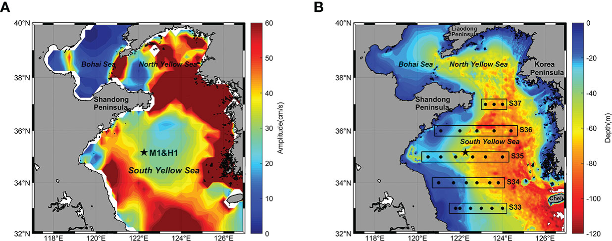
Figure 1 M2 tidal current amplitude and topography of the South Yellow Sea (SYS) and the location of different in situ observations. M1 and H1 with the same site, indicated by the black star. (A) The amplitude of M2 tidal current from TPXO7 global tidal model in which the tidal currents are stronger. (B) The topography and geography of the SYS. The color contours denote bathymetry. The black dots in the rectangles show the CTD casts along five latitudinal sections (S33-S37) in the cruise survey.
2.2. Satellite data
Multisource satellite observations are used as input data, including absolute dynamical topography (ADT), SST, SSS, and SSW. The SSW contains u and v components (USSW, VSSW). The ADT data are provided by SSALTO/Data Unification and Altimeter Combination System (DUACS) and were available through the Copernicus Marine Environment Monitoring Service (CMEMS, https://marine.copernicus.eu/). The product merged multiple L3 along-track measurements and conducted the tidal corrections (Taburet et al., 2019). The SST data are obtained from Daily Optimum Interpolation Sea Surface Temperature (DOISST, https://psl.noaa.gov/), developed by National Oceanic and Atmospheric Administration Physical Sciences Laboratory (NOAA PSL). It is a blend of in situ SST with satellite SST derived from the Advanced Very High Resolution Radiometer (Banzon et al., 2016; Huang et al., 2021). The SSS data are obtained from SMOS L3OS 2Q Debiased daily valid ocean salinity values product (https://sextant.ifremer.fr/), which are distributed by Centre Aval de Traitement des Données SMOS (CATDS) and corrected the offshore SSS through various in situ observations (Boutin et al., 2018). The SSW data are provided by the Cross-Calibrated Multi-Platform (CCMP; https://rda.ucar.edu/datasets/ds745.1/). The CCMP uses a variational analysis method to smoothly fuse multisource surface wind data into the gridded data at 6 hours intervals (Atlas et al., 2011). The temporal resolution of the CCMP data is 6 hourly while the rest is daily, and the spatial resolution of all these data is 0.25°×0.25°.
2.3. Tide model data
We coupled the tide model data into the inputs of machine learning model. The tide model data, including surface tidal elevation and tidal currents, are estimated by the TPXO7 global tidal model provided by Oregon State University, which was built hourly on a 0.25°×0.25° grid. The tide model is based on the hydrodynamic equation and uses the generalized inversion method to assimilate the measured data, including satellite altimetry data and tide observations. Furthermore, it was recently used for the hydrographic study in the YS (Bi et al., 2021; Lin et al., 2021; Sun et al., 2022). The M2 tide is the most dominant tidal component in the SYS, having stronger tidal current (Figure 1A). The tides have complex structures in the SYS, which is detrimental to temperature inversion. In this study, the tidal time series of eight basic tidal components (M2, S2, N2, K2, K1, O1, P1, and M4) are extracted by the Matlab Tide Model Driver toolbox (https://www.esr.org/research/polar-tide-models/tmd-software/). The tide model data and satellite observations, which have the same spatial resolution, were co-located with the temperature profiles by the nearest neighbour method, and the temporal resolution is unified to daily.
2.4. ARMOR3D dataset
We also validate the temperature estimation with the ARMOR3D dataset (Guinehut et al., 2012), which was obtained through CMEMS. The ARMOR3D used multiple linear regression and optimal interpolation, providing the weekly temperature and salt fields at 0.25° × 0.25° resolution over 15 regularly spaced vertical levels between surface and 80 m depth. The weekly averaged three-dimensional temperature field in April, July and October 2019 from ARMOR3D is used to compare. The YSCWM below the thermocline is clearly visible in the observation-based ARMOR3D data (Figure 2A). In addition, the M1 temperature data are used to evaluate ARMOR3D. In order to match the temporal resolution, the M1 data are first calculated as weekly average and then compared to the nearest neighboring grid in ARMOR3D. As shown in Figure 2B, most of the data points are distributed along the equal line with low bias, absolute error and high Pearson’s correlation coefficient. The evident seasonal temperature variations in ARMOR3D are well simulated compared to the M1 observations (Figures 2C, D). Even though ARMOR3D presents a shallower mixed layer and a more durable YSCWM which lasts until October, it well reproduces the vertical thermal structure at the M1 station and is worth to refer for the thermal structure of SYS.
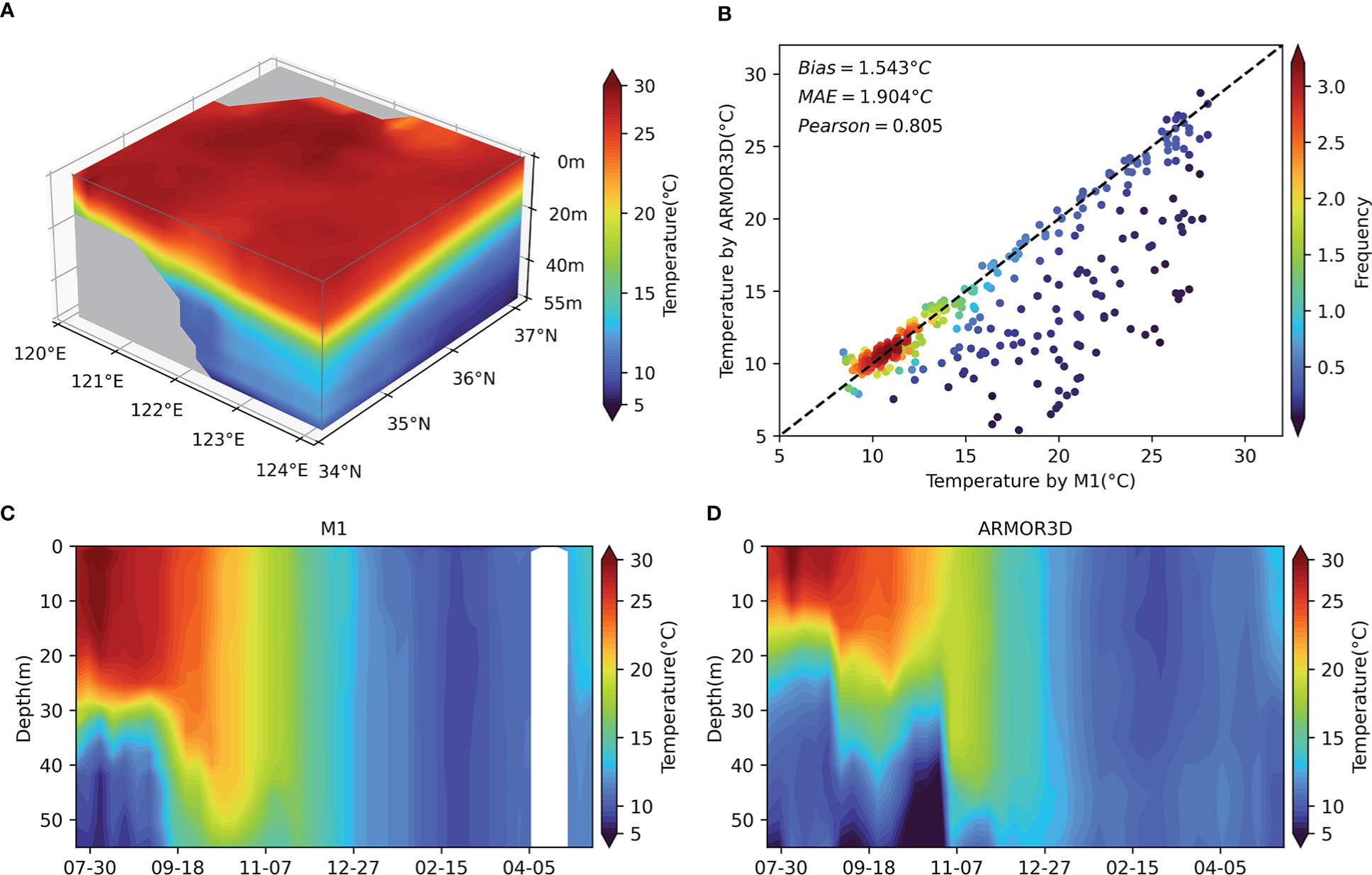
Figure 2 YSCWM phenomena in ARMOR3D temperature data and comparison of ARMOR3D, M1 temperature field at M1 location during July 2019 to May 2020. (A) The distribution of weekly average surface and subsurface temperature (°C) in the SYS with a spatial resolution of 0.25°×0.25° between 25 July and 31 July 2019 from the ARMOR3D data, selecting 0-55 m depth to correspond to the M1 data. The YSCWM is below the thermocline. (B) Scatter plots for M1 temperature and ARMOR3D temperature from all depth. (C) Weekly average temperature data from M1 with gaps representing interruptions in the measurements. (D) ARMOR3D temperature fields at M1 site.
3. Methods
3.1. Gaussian mixture model clustering
Considering the large seasonal variation of the thermal structure in the SYS, we use unsupervised GMM clustering techniques to shrink the sample space and improve the accuracy (Landschutzer et al., 2013; Parard et al., 2015). As a probabilistic model, GMM is often used for data clustering (Attal et al., 2015). First, the GMM randomly initializes the Gaussian distribution parameters of each cluster. Then the posterior probability of each sample is calculated and used to compute the new Gaussian distribution parameters. The process is repeated until the expectation function is maximized. Compared with the K-means method, GMM is more suitable for non-spherical clusters with different sizes and densities (Wang et al., 2019; Askari, 2021). Therefore, it is appropriate for the classification of ocean temperature profiles (Maze et al., 2017; Sambe and Suga, 2022). GMM requires the number of classes (K) as an input parameter. Therefore, the Davies-Bouldin index (DBI) is used to determine the appropriate number of classes in this study. The number of classes having the minimized DBI is considered the optimal result. Since the initial values of the Expectation-Maximization algorithm are randomized, the GMM clustering was applied 20 times, and 80% of the data were randomly selected from the M1 and H1 data each time to stabilize the clustering results. Figure 3 shows the DBI from clustering results with different K. As a result, we judge that stable and good clustering results could be obtained if K = 3. The clustering results are shown in Figure 4. Although the YSCWM temperature structure from H1 data is still growing, it is approaching maturity. Therefore, they are named after a specific stage of YSCWM: the maturity stage, the declining stage, and the disappearance stage. During the maturity stage of YSCWM with weaker wind, the sea surface is subjected to strong thermal radiation, forming a stable upper mixed layer and a strong thermocline, which prevents heat transfer, so the bottom water stays cold (Lee et al., 2016). It leads to a multi-layer temperature structure in the SYS, with a large temperature difference between the sea surface and the bottom (Figure 4A). In the YSCWM declining stage, the cooling at the sea surface and stronger mixing lead to a thicker and colder upper mixed layer and the subsequent weakening and deepening of the thermocline (Figure 4B). Meanwhile, critical tidal currents raise the temperature at the bottom layer then decline the YSCWM (Li et al., 2016). Thermal forcing at the air-ocean interface and agitation by strong winds together cause strong vertical mixing, forming a well-mixed low temperature structure (Figure 4C) from the sea surface to the bottom in the YSCWM disappearance stage (Chu et al., 1997).
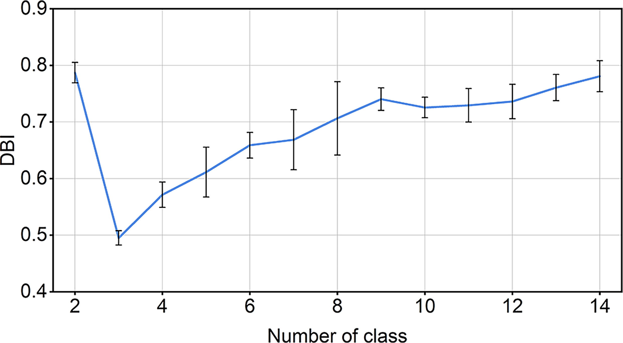
Figure 3 The mean value (the blue line) and confidence intervals (one σ, the black error bar) of the Davies-Bouldin index (DBI) from 20 trials of Gaussian mixture model (GMM) clustering for the different number of classes.
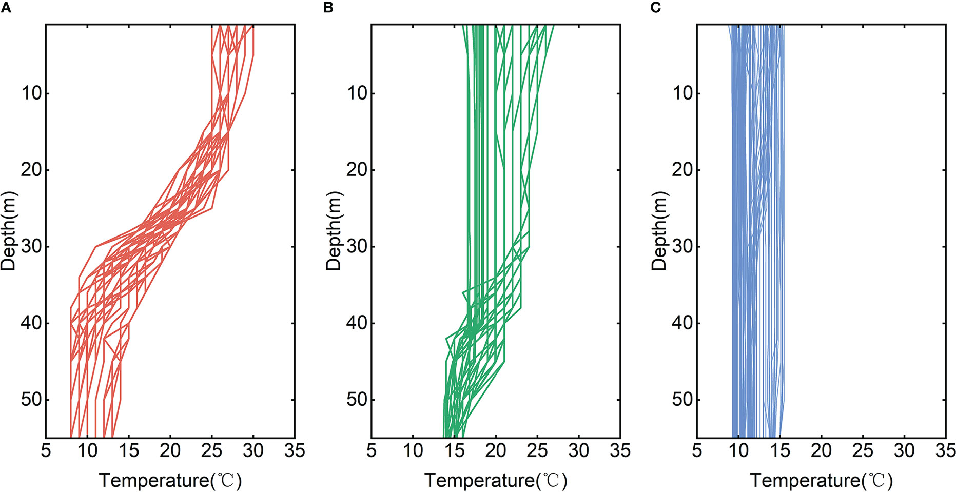
Figure 4 Vertical temperature structure of the classified profiles from M1 data, which represents different stages of the YSCWM: (A) the maturity stage, (B) the declining stage, and (C) the disappearance stage.
3.2. Light gradient boosting machine
To tackle the limitations of small data and complex computations, we adopt the LGBM algorithm to predict the temperature by taking advantage of its lightweight. LGBM is a gradient boosting framework based on decision trees, which has been well used in the marine field and shown a faster training speed and higher accuracy for small data (Su et al., 2021; Dong et al., 2022). Same as the other boosting algorithms, it sums the results of multiple decision trees as the final prediction output. Gradient-based One-Side Sampling (GOSS) and Exclusive Feature Bundling (EFB) are two important features of LGBM. The GOSS excludes most of the samples with small gradients and calculates the precise information gain by the remaining samples. The EFB approach integrates many mutually exclusive features and reduces the data dimension. To build a better model, the Bayesian optimization strategy is used to optimize several important parameters of LGBM. The optimization method is a Gaussian process with a faster speed. According to previous studies, three essential hyperparameters need to be adjusted: the number of leaf nodes (num_leaves), the learning rate, and the number of iterations (n_estimators). The bounds of n_estimators were set 100 and 1000, and the best n_estimators is 400 without overfitting. It improves the accuracy by 16.6% compared to n_estimators=100. However, the accuracy at n_estimators=1000 is only increased by 0.1% compared to the best n_estimators. When the learning_rate is increased to 0.01 from 0.001, the performance is improved by 21% compared to the starting learning_rate=0.001, but the effect does not enhance when it is increased further until 0.1. The test range of num_leveas is from 5 to 30. The performance of the model at the best num_leveas=5 improved by 3.4% over num_leveas=30. The optimal parameters are shown in Table 1. In addition, the max depth is set to 5, to prevent overfitting due to excessive complexity of the model. The other parameters are set to default values.
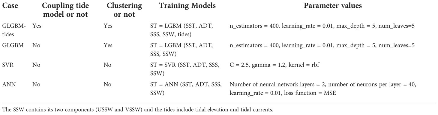
Table 1 Design of experiments and parameter values.
3.3. Experimental setup
First, we input the eight harmonic components (M2, S2, N2, K2, K1, O1, P1, and Q1), geographic location and time parameters into the TPXO7.2 global tidal model, to extract tidal elevation and tidal currents data. TPXO7.2 fits best the Laplace tidal equation in the least squares sense. Second, the datasets consisting of tide model data, satellite observations and in situ temperature profiles are divided into three different stages by GMM clustering. The surface parameters (ADT, SST, SSS, SSW, tidal elevation, and tidal currents) are used as independent input variables and the temperature time series are used as labels to prepare the training and test data. To ensure that the training and test sets have a similar seasonal distribution, all samples at the location of M1 are normalized and randomly sampled into the training set (60%) and the test set (40%) by month (Figure 5). Third, the model is tuned and trained using the Bayesian optimization method to obtain suitable temperature estimators at 17 depth levels. Figure 6 shows the technique flowchart of one stage at a certain depth. We use a total of 162 samples to train and 114 samples to test when using mooring observations for validation. Finally, temperature predictions are applied to a larger horizontal space and verified with cruise observations in the SYS where the number of training data and evaluating data are 276 and 78, respectively.
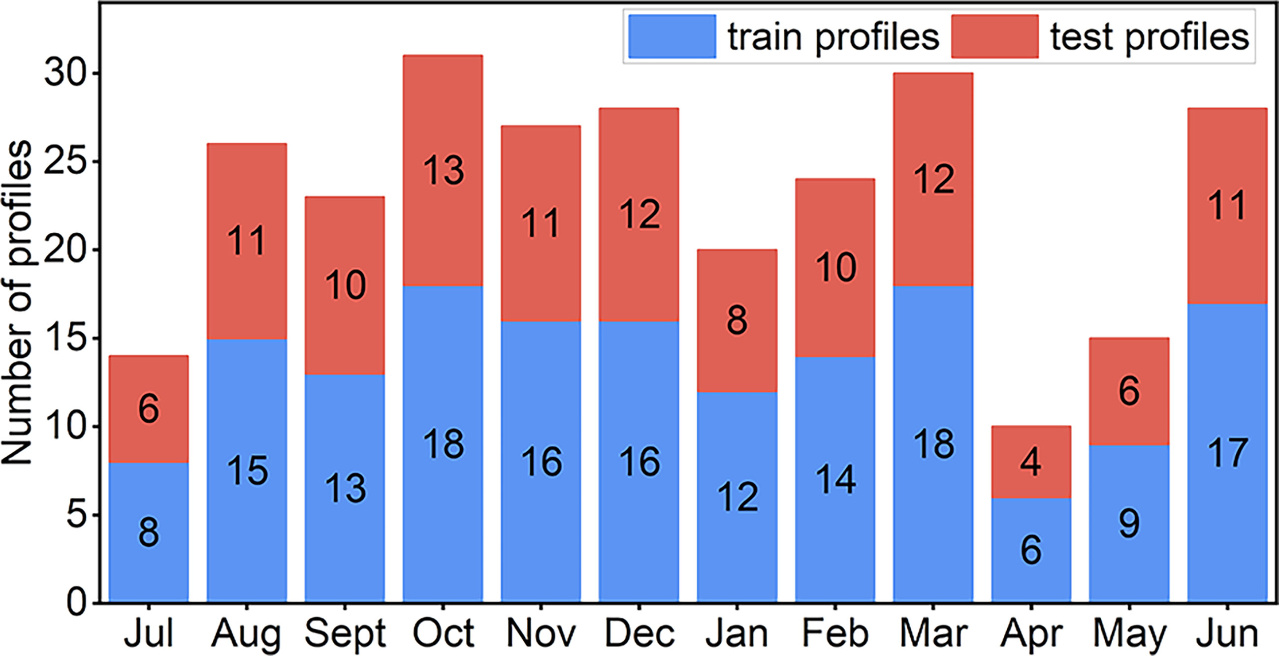
Figure 5 Monthly distribution of the number of temperature profiles from M1 and H1 data.
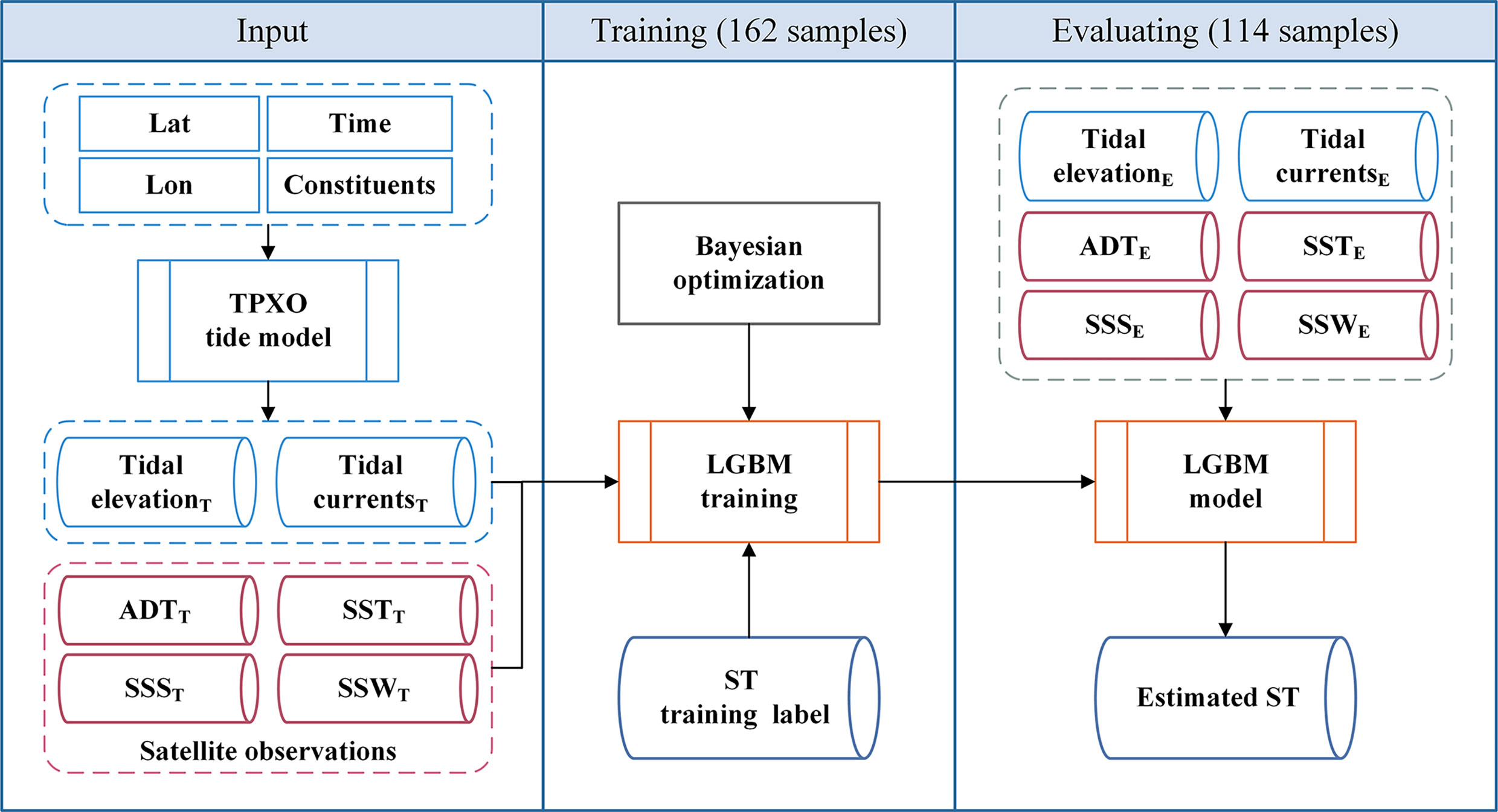
Figure 6 Flowchart of the subsurface temperature (ST) estimation at different depth levels using LGBM models for a certain class. In the moored buoy observation validation, a total of 162 samples were used for training and 114 samples for testing. In the cruise survey validation, the training data and validation data are 276 and 78, respectively.
To evaluate the tide model coupled temperature inversion method, we designed comparative trials named GLGBM-tides and GLGBM. They both use the LGBM method with pre-clustering process but the former couples the tide model while the latter does not. Additionally, we compared other reconstruction methods. Case SVR and Case ANN use Support Vector Regression (SVR) model and Artificial Neural Network (ANN) model, respectively. Table 1 summarizes the different trials. These are optimized by the Bayesian optimization strategy, and the parameters of different models are shown in Table 1. The ARMOR3D dataset is also used for comparison.
4. Results and discussion
The sea surface data of the test samples are input into the different models to obtain the reconstructed vertical temperature structure. Based on the test data, we first examine the importance of tides in offshore temperature prediction from the time series data. Then the performance of the different models is compared. Finally, we estimate the temperature structure of each latitude section (S33-S37) and compared it with the ARMOR3D dataset.
4.1. The performance of tide model data on the temperature field reconstruction
Previous studies have shown that strong tidal mixing has an important effect on the temperature structure and enhances vertical heat exchange in the water column during summer in the YS (Lü et al., 2010; Yao et al., 2012; Li et al., 2016; Yu et al., 2016). Here, we first compared GLGBM-tides and GLGBM to investigate how tides affect temperature estimation in this study. Figure 7 shows the comparison between the temperature profiles obtained by the two models and in situ observations. The profiles are randomly selected according to spring tide and neap tide in the maturity stage of YSCWM. In this stage, bottom vertical disturbances are stronger (Li et al., 2016), which affects the heat transfer and thermal structure significantly. Besides, the air-sea heat flux and the cooling process of the previous winter strongly influences the intensity of YSCWM (Zhu et al., 2018). This leads to machine learning models having more difficulty accessing these temperature variations and more considerable differences between in situ and estimated temperature (Figure 7). However, it can be seen that the temperature profiles obtained from GLGBM-tides are more consistent with the measured profiles, especially deeper than 30 m. This confirms that the method coupled with tide model can effectively improve the structure of the predicted temperature profiles during the maturity stage. To further validate the above results, several evaluation indicators metrics are used to assess the two models. Except for root mean square error (RMSE), coefficient of determination (R2) and absolute difference, the error (defined as the proportion of RMSE in the actual mean temperature observations) is also used to evaluate the accuracy and reliability of the model. The evaluation indicators are computed as follows:
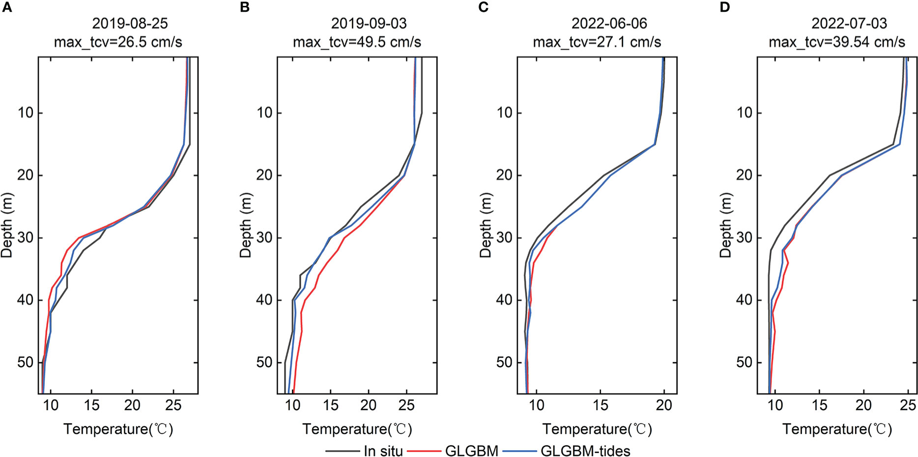
Figure 7 Comparison among the vertical structure of temperature at depths of 1-55 m obtained by observed ST (black), GLGBM-tides (blue) and GLGBM (red) during maturity stage of the YSCWM. The profiles are randomly selected according to spring tide (B, D) and neap tide (A, C). The max_tcv represents the daily maximum tidal current speed.
Here, Ti denotes the observed temperature while is the estimated temperature by models. The is the mean values of Ti over the whole observation. N is the number of test samples.
From Figures 8A-C, the evaluation indicators of the two methods are similar within the 1-28 m depth layer. However, in the 40 m depth level, the RMSEs of the two are 0.806 and 0.863, respectively. Meanwhile, the accuracy of other layers has been improved by different degrees from 30 m to 55 m. Figure 8D shows that the smaller absolute errors occupy a larger proportion in the GLGBM-tides model. In addition, the enhancement is mainly manifested during the maturity stage (Figure 9). It may be attributed to the tidal mixing primarily influencing the range up to 30 m from the bottom during summer (Qiao et al., 2004b). In this trial, GLGBM-tides coupled the tide model while GLGBM not. Meanwhile, strong tides affect the heat transfer and thermal structure of the profile, especially the bottom layer. As a result, GLGBM-tides better learn the temperature variation affected by tidal mixing, and it presents a more consistent vertical thermal structure with in situ observations (Figure 7) and better performance than GLGBM (Figure 8).
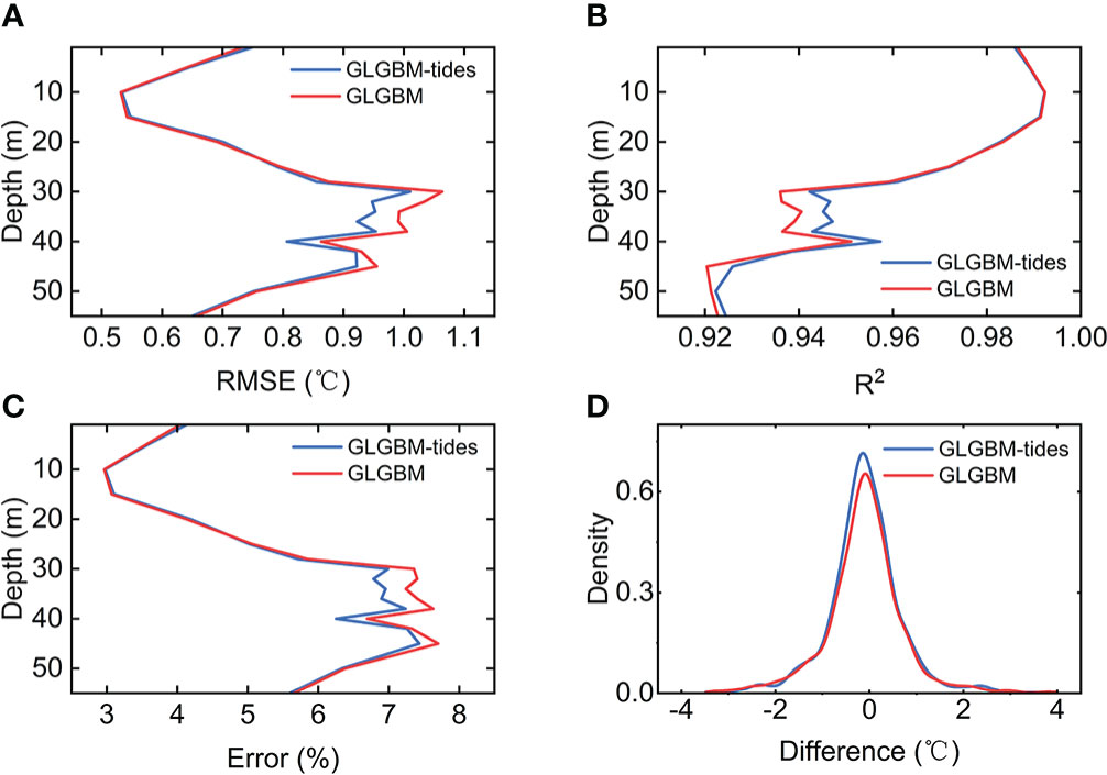
Figure 8 The average RMSE (A), R2 (B), Error (C) at the 17 depth levels and absolute difference density distribution (D) between the test datasets and estimated ST from GLGBM-tides (blue) and GLGBM (red).
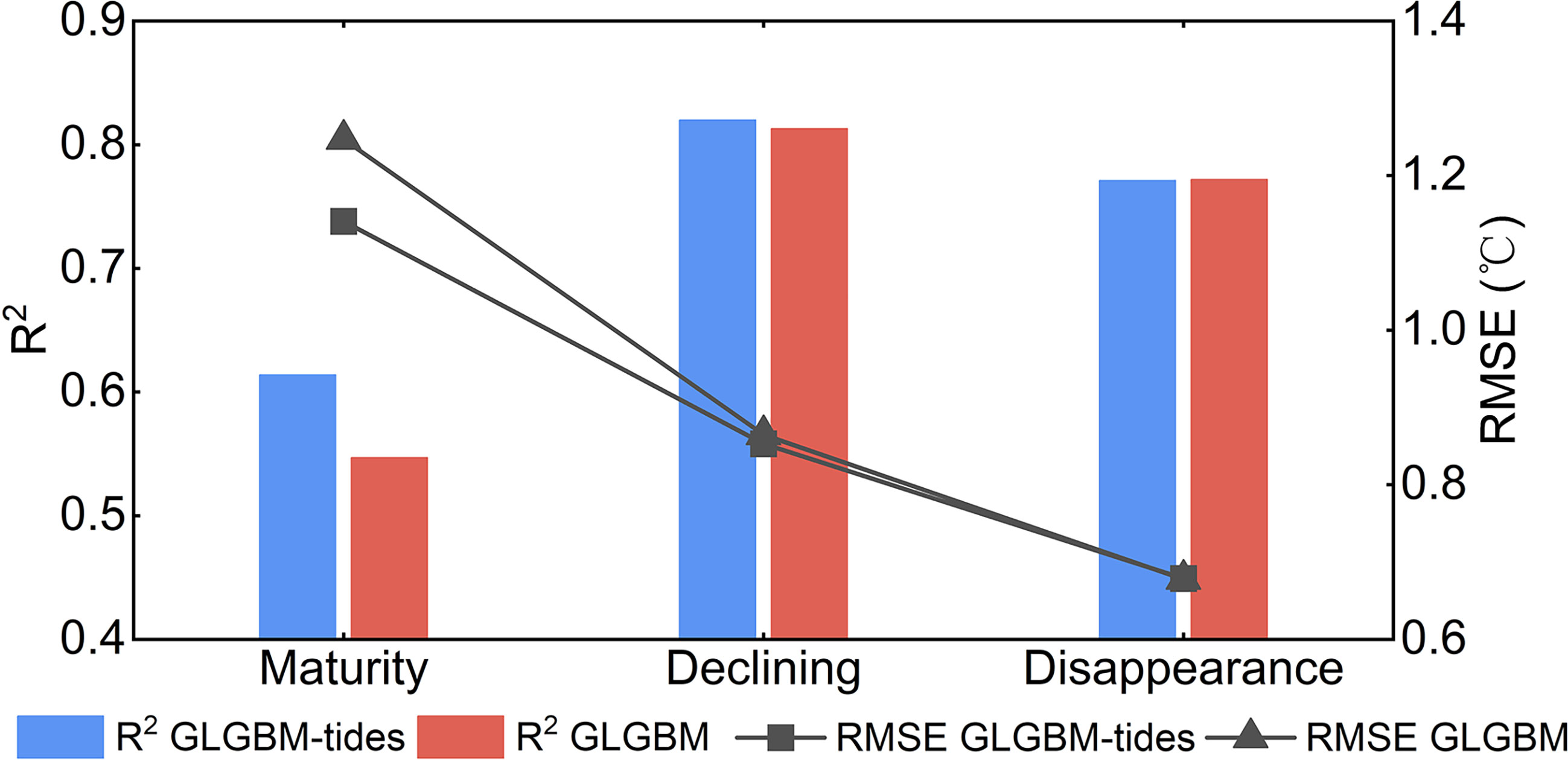
Figure 9 The average RMSE and R2 between 30 and 50 m depth using GLGBM-tides and GLGBM in three YSCWM stages (the lines indicate the RMSE and the bars indicate the R2).
Furthermore, we analyzed the accuracy of the models at three specific stages from 30 m to 50 m (Figure 9). The averaged R2 and RMSE are significantly different in the maturity stage of YSCWM and similar in the decline and disappearance stages. It performs less well in the maturity stage than the other two stages in the YSCWM deep. Strong stratification leads to a large difference in temperature between YSCWM and the upper layer. Besides, YSCWM is influenced not only by the air-sea heat flux but also by the cooling process of the previous winter (Zhu et al., 2018). It means that the thermal structure of YSCWM is more difficult to be described by sea surface parameters in the machine learning models hence lower R2 and higher RMSE. The averaged R2 of GLGBM-tides and GLGBM are 0.614/0.547, with approximately 12% improvement. It results from the stronger influence of tidal mixing on the temperature structure in summer. Therefore, tides are worth considering in the offshore temperature field reconstruction.
Overall, the GLGBM-tides has good accuracy with errors of less than 8% at all depth layers and most absolute difference of less than 2°C (Figures 8C, D). It is worth noting that a bump appears above 30 m in Figure 8B. This phenomenon may be related to the depth of the mixed layer. According to previous research, the depth of the mixed layer in SYSCWM is about 5-25 m (Qiao et al., 2004b). The temperature does not vary significantly within the mixed layer, which causes the lower RMSE and higher R2. The tidal mixing primarily influences the range up to 30 m from the bottom, enhancing the vertical temperature variability (Qiao et al., 2004a) and the particular structure of the YSCWM makes it difficult for the model to accurately describe the temperature variations. Therefore, the accuracy of reconstruction at these depths will be worse (Figures 8A-C).
It helps to understand the different effects of each sea surface parameter on the ST, by analyzing the importance of sea surface parameters at different depths. The LGBM reflects the importance of different features by calculating the number of times the sea surface parameters are used to segment the data across all trees. The relative importance of each parameter is calculated by summing and normalizing the feature importance from the LGBM. Figure 10A shows the relative importance of each sea surface parameter from GLGBM-tides. According to previous studies, the vertical thermal structure in the Yellow Sea (YS) is influenced by air-sea heat flux, the wind, tidal vertical mixing, and freshwater input (Chu et al., 1997). The temperature in the mixed layer is vertically quasi-uniform due to the mixing of multiple dynamic processes, such as wave motion and wind. Meanwhile, the mixed layer gradually thickens from the maturity stage to the disappearance stage of YSCWM, which means that the sea surface temperature (SST) can explain more subsurface temperature variations. Consequently, SST is the main driver of the model, with a more than 30% contribution at 17 depth levels (Figure 10A). However, below the mixed layer, the heat transfer is blocked, and it is difficult to explain the temperature change by relying on SST alone. Therefore, the trend of SST contribution decreases with deepening (Figure 10A).
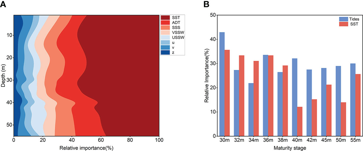
Figure 10 The relative importance of each sea surface parameters in three stages and maturity stage at different depths. (A) Average relative importance by three stages of all input parameters. The parameters of tides include tidal elevation (z) and tidal currents (u, v). (B) The relative importance of the SST and tides in YSCWM maturity stage below 30 m.
Warming or cooling mainly drives density changes, causing sea level changes since salinity variation is not significant in the SYS. There is a close correlation between ADT and subsurface thermal structure. The sea level variations are influenced more significantly by those depths where temperature sharply changes, such as the thermocline. Therefore, the ADT contribution is higher at those depths where the temperature fluctuates drastically (Figure 10A), such as the thermocline in the maturity and declining stages and the bottom layer affected by tides. It leads to an average relative importance of 10% and 16% for ADT above and below 15 m depth, respectively.
SSS and SSW are also important parameters (Wu et al., 2012; Klemas and Yan, 2014; Su et al., 2015). The SSS is related to freshwater input (Nieves et al., 2014), which causes density anomalies and then affects the dynamics. The contribution of SSS is less variable from surface to 40 m depth but increases at the bottom (Figure 10A). This may be related to the Yellow Sea Warm Current (YSWC) in the winter, which brings a more salty and warmer water mass, especially at the bottom and manifests in the SSS. Wind forcing changes sea level and also affects ocean mixing, intensifying heat exchange between layers. Southerly winds prevail in summer and northerly winds during winter in the SYS, which causes VSSW to contribute more than USSW (Figure 10A). The vertical distribution of the wind (USSW and VSSW) contribution is roughly same but increases slightly at the bottom (Figure 10A), which is due to the mixed layer deepening during the declining stage of YSCWM.
Tide-induced mixing causes changes in the ocean heat vertical distribution. Even though the overall tidal contribution is weak and less variable, it may be important for a particular stage. During the maturity stage of YSCWM, the tides contribution (u, v, and z in Figure 10A) is about 15% within the mixed layer but can exceed 30% below the mixed layer (Figure 10B) causing the tidal-induced mixing mainly affects the bottom and above 30 m range (Qiao et al., 2004b). It is comparable to the SST contribution (Figure 10B).
4.2. Comparison with other methods
We compared other temperature prediction methods. The SVR and ANN methods have no pre-clustering process and tides. The overall R2 of SVR and ANN are 0.862/0.888 with the RMSE of 1.506/1.22°C, respectively on the time series. It shows that the GLGBM coupled tides have better accuracy from Figures 11A-C. However, the ANN has similar accuracy above 20 m compared to GLGBM-tides, which may be related to the dominance of SST in this depth range. Additionally, GLGBM-tides allows errors to be smaller and more concentrated, effectively improving model performance, as revealed by the error density distribution (Figure 11D).
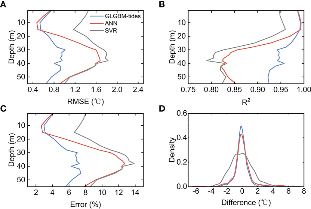
Figure 11 The average RMSE (A), R2 (B), Error (C) at the 17 depth levels and absolute difference density distribution (D) between the test datasets and estimated ST from GLGBM-tides (blue), ANN (red) and SVR (grey).
We choose H1 data to demonstrate the performance of different methods for fine and continuous data. Since deep learning is more applicable to large data, ANN performs unstable. We implement ANN 20 times to obtain the average temperature estimation. Figure 12 shows the observation from H1 and the reconstructed temperature structure from different methods. The seasonal warming in the upper mixed layer has been reproduced by all methods. Here we adopt the upper boundary of the thermocline as the mixed layer depth (MLD) to further evaluate the performance of models. The reconstructed temperature fields are interpolated to 1 m vertical resolution before calculating MLD. The results show that the MLD is maintained around 10-15 m in the H1 observations (Figure 12A). For the reconstructed temperature field by GLGBM-tides (Figure 12B), the MLD changed generally consistent with the H1 observation. Influenced by atmospheric processes, the MLD becomes shallower from 17 June to 1 July. This process is well reproduced by GLGBM-tides. Reconstructions from other methods failed to capture this variation. The MLD from reconstructed temperature by ANN is stabilized at about 15 m (Figure 12C) while the MLD reconstructed by SVR (Figure 12D) is too deep. The reconstructed temperature from ANN can indicate the trend of YSCWM but has large noises (Figure 12C). The temperature field estimated from SVR fails to reproduce the strong thermocline and YSCWM (Figure 12D). GLGBM-tides can reproduce the vertical temperature structure well compared to the observations. However, the overall estimate of the YSCWM by GLGBM-tides is slightly warmer than the observations from surface to bottom. Hence, the intensity of YSCWM from estimation is weaker. It is noticeable that the reconstruction of the thermocline is well, which assists in predicting the depth of the YSCWM.

Figure 12 Comparison H1 observations (A) and reconstruction from GLGBM-tides (B), ANN (C) and SVR (D) from 0-50 m in H1 period. The MLD is indicated by the solid black line.
We attempt to apply the temperature estimation at the locations of the cruise observations by training the samples from H1 and M1 and use S33-S37 data for verification. The ARMOR3D reanalysis data is used to compare as well. The temperature estimation beyond the topography is deleted. Figure 13 shows the temperature structure of 35°N and 36°N sections (S35 and S36) in three stages of YSCWM. The overall RMSE by all samples of GLGBM-tides and ARMOR3D is 1.781/2.133°C, respectively. It is higher than above due to the spatial heterogeneity of the thermal structure in SYS but the reconstructed vertical temperature structure is still in general agreement with the observations. In the mixed layer, the reconstructed temperature was colder than observation while the ARMOR3D is warmer and the reconstruction has a small zonal variation. It is the result of the training data containing inadequate spatial features. In contrast, the reanalysis data shows a clear spatial difference for fully considering spatial features during production but shows a shallower mixed layer, such as Figures 13B, D. In the declining and disappearance stages, the temperature reconstruction is better for the strong mixing but the ARMOR3D still shows a significant temperature gradient from surface to 35 m depth (Figures 13C, D). The estimates provide a better reconstruction of the thermocline than ARMOR3D (Figures 13A, B). The intensity of the thermocline in the ARMOR3D data is strong (Figures 13A, B) in maturity stage while it is weak in declining stage (Figures 13C, D). The estimated temperature of YSCWM by the GLGBM-tides is slightly warmer especially in the declining stage (Figures 13C, D), but consistent in terms of depth and spatial distribution. The ARMOR3D have the shallower upper boundary of the YSCWM so the temperature of YSCWM is cold as observations (see Figure 13B). Both have good reconstruction of well-mixed temperature structure in the disappearance stage (Figures 13E, F). However, the cold cores in S36 could be observed (Figures 13B, D, F) by cruise data but this special structure is difficult to reproduce. Figure 14 shows the spatial distribution of RMSE in three stages. The accuracy of the proposed method is good from 121°E to 123.5°E. From Figure 14A, the RMSE increases from the center (location of M1) along longitude towards the sides, but with larger differences in farther regions, which may stem from the sparseness of the offshore observations. On the contrary, the RMSE of ARMOR3D decreases gradually from the center to the outside but is similar on the west side of the study area. However, the GLGBM-tides and ARMOR3D have close overall R2, which are 0.927 and 0.884, respectively. Generally, our reconstruction results are reliable through comparison with ARMOR3D data.
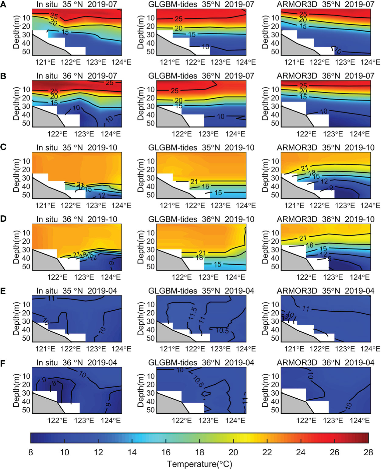
Figure 13 Comparison of vertical temperature distributions of in situ observations (left), reconstruction from GLGBM-tides (middle) and ARMOR3D (right) in 0-55 m along the 35°N and 36°N section at maturity stage (A, B), declining stage (C, D) and disappearance stages (E, F) of YSCWM.

Figure 14 Spatial distribution of the overall RMSE by depths from GLGBM-tides (A) and ARMOR3D (B). The red star indicates the location of the M1 and H1.
5. Conclusion
This paper proposed the offshore temperature reconstruction method coupled TPXO tide model based on LGBM, using sea surface parameters (ADT, SST, SSS, SSW, tides). The performance of model incorporating tides is quantitatively analyzed. In addition, the temperature estimation is applied spatially and compare with other ARMOR3D. The primary significance of this study is as follows:
(1) The SYS is a typical offshore sea with a huge tidal range, resulting in the difficulty of temperature prediction by classic machine learning method. We coupled the tide model by feeding the estimated tidal elevation and tidal currents by the tide model into a lightweight ensemble learning approach to retrieve SYS thermal structure using small data. The method can generate continuous 3D temperature field at 0-55 m in the SYS at daily and 0.25° × 0.25° resolution. Experiments demonstrate that proposed method increases the R2 by 12%, compared to GLGBM and the model tide data mainly improves the accuracy below thermocline in the maturity stage of YSCWM. It has significance for the depth prediction of the YSCWM. Meanwhile, the contribution of tides is comparable with SST in the temperature reconstruction model. The proposed method provides a new explorable direction for reconstructing the offshore thermal structure.
(2) The proposed method is also compared with other machine learning approaches and ARMOR3D dataset. Time series experiments show that the proposed method is superior to SVR and ANN with the RMSE of 0.803°C, 1.506°C, and 1.22°C, respectively. Compared with the cruise data, the method has good and stable results in the three stages of YSCWM. Around the location of M1, the RMSE and R2 have a good performance in our experiments so our method is effective in the SYS. Furthermore, the temperature reconstruction is comparable to observation-based ARMOR3D dataset, with close R2 although their RMSE differed in spatial distribution.
Due to the small samples, important oceanic phenomena at longer time scales and larger spatial scales may not be well represented in the reconstructed temperature fields. With sufficient data, better accuracy will be obtained on larger spatial and temporal scale. Therefore, extending the data over longer time and more space to improve the prediction performance of the model is a priority for future work.
Data availability statement
The original contributions presented in the study are included in the article/Supplementary Materials. Further inquiries can be directed to the corresponding author.
Author contributions
All authors conceived the research question. FY and JL conducted the analysis on the datasets of the in situ observations. FY and GC led the design of the inversion model. FS performed the run of the model. FY and FS wrote the first draft and all authors reviewed and edited the final manuscript. All authors contributed to the article and approved the submitted version.
Funding
This research was jointly supported by the following programs: (1) the Laoshan Laboratory science and technology innovation projects (No. LSKJ202204304); and (2) the Key Laboratory of Marine Science and Numerical Modeling, Ministry of Natural Resources (Grant No. 2021-ZD-01) and (3) the National Natural Science Foundation of China (Grant No. 41806190).
Acknowledgments
The study is benefited from the cruise dataset collected onboard of R/V Lanhai 101 implementing the open research cruise NORC2020-01 supported by NSFC Shiptime Sharing Project.
Conflict of interest
The authors declare that the research was conducted in the absence of any commercial or financial relationships that could be construed as a potential conflict of interest.
Publisher’s note
All claims expressed in this article are solely those of the authors and do not necessarily represent those of their affiliated organizations, or those of the publisher, the editors and the reviewers. Any product that may be evaluated in this article, or claim that may be made by its manufacturer, is not guaranteed or endorsed by the publisher.
References
Ali M. M., Swain D., Weller R. A. (2004). Estimation of ocean subsurface thermal structure from surface parameters: A neural network approach. Geophys. Res. Lett. 31, L20308. doi: 10.1029/2004GL021192
Askari S. (2021). Fuzzy c-means clustering algorithm for data with unequal cluster sizes and contaminated with noise and outliers: Review and development. Expert Syst. Appl. 165, 113856. doi: 10.1016/j.eswa.2020.113856
Atlas R., Hoffman R. N., Ardizzone J., Leidner S. M., Jusem J. C., Smith D. K., et al. (2011). A cross-calibrated, multiplatform ocean surface wind velocity product for meteorological and oceanographic applications. B. Am. Meteorol. Soc 92, ES4–ES8. doi: 10.1175/2010BAMS2946.2
Attal F., Mohammed S., Dedabrishvili M., Chamroukhi F., Oukhellou L., Amirat Y. (2015). Physical human activity recognition using wearable sensors. Sensors-Basel 15, 31314–31338. doi: 10.3390/s151229858
Banzon V., Smith T. M., Chin T. M., Liu C., Hankins W. (2016). A long-term record of blended satellite and in situ sea-surface temperature for climate monitoring, modeling and environmental studies. Earth System Sci. Data 8, 165–176. doi: 10.5194/essd-8-165-2016
Bi C., Yao Z., Bao X., Zhang C., Ding Y. A., Liu X., et al. (2021). The sensitivity of numerical simulation to vertical mixing parameterization schemes: a case study for the yellow Sea cold water mass. J. Oceanol. Limnol. 39, 64–78. doi: 10.1007/s00343-019-9262-y
Boutin J., Vergely J. L., Marchand S., D’Amico F., Hasson A., Kolodziejczyk N., et al. (2018). New SMOS Sea surface salinity with reduced systematic errors and improved variability. Remote Sens. Environ. 214, 115–134. doi: 10.1016/j.rse.2018.05.022
Chu P. C., Fralick C. R., Haeger S. D., Carron M. J. (1997). A parametric model for the yellow Sea thermal variability. J. Geophys. Res. 102, 10499–10507. doi: 10.1029/97JC00444
Diao X., Si G., Wei C., Yu F. (2022). Structure and formation of the south yellow Sea water mass in the spring of 2007. J. Oceanol. Limnol. 40, 55–65. doi: 10.1007/s00343-021-0206-y
Dong L., Qi J., Yin B., Zhi H., Li D., Yang S., et al. (2022). Reconstruction of subsurface salinity structure in the south China Sea using satellite observations: A LightGBM-based deep forest method. Remote Sens. Basel 14, 3494. doi: 10.3390/rs14143494
Guinehut S., Dhomps A. L., Larnicol G., Le Traon P. Y. (2012). High resolution 3-d temperature and salinity fields derived from in situ and satellite observations. Ocean Sci. 8, 845–857. doi: 10.5194/os-8-845-2012
Guo Y., Mo D., Hou Y. (2021). Interannual to interdecadal variability of the southern yellow Sea cold water mass and establishment of “Forcing mechanism bridge”. J. Mar. Sci. Eng. 9, 1316. doi: 10.3390/jmse9121316
Huang B. Y., Liu C. Y., Banzon V., Freeman E., Graham G., Hankins B., et al. (2021). Improvements of the daily optimum interpolation Sea surface temperature (DOISST) version 2.1. J. Climate 34, 2923–2939. doi: 10.1175/JCLI-D-20-0166.1
Hwang J. H., Van S. P., Choi B. J., Chang Y. S., Kim Y. H. (2014). The physical processes in the yellow Sea. Ocean Coast. Manage. 102, 449–457. doi: 10.1016/j.ocecoaman.2014.03.026
Klemas V., Yan X. (2014). Subsurface and deeper ocean remote sensing from satellites: An overview and new results. Prog. Oceanogr. 122, 1–9. doi: 10.1016/j.pocean.2013.11.010
Landschutzer P., Gruber N., Bakker D., Schuster U., Nakaoka S., Payne M. R., et al. (2013). A neural network-based estimate of the seasonal to inter-annual variability of the Atlantic ocean carbon sink. Biogeosciences 10, 7793–7815. doi: 10.5194/bg-10-7793-2013
Lee J. H., Pang I. C., Moon J. H. (2016). Contribution of the yellow Sea bottom cold water to the abnormal cooling of sea surface temperature in the summer of 2011. J. Geophys. Res. 121, 3777–3789. doi: 10.1002/2016JC011658
Li J., Jiang F., Wu R., Zhang C., Tian Y. J., Sun P., et al. (2021). Tidally induced temporal variations in growth of young-of-the-Year pacific cod in the yellow Sea. J. Geophys. Res. 126, e2020JC016696. doi: 10.1029/2020JC016696
Li J., Li G., Xu J., Dong P., Qiao L. L., Liu S. D., et al. (2016). Seasonal evolution of the yellow Sea cold water mass and its interactions with ambient hydrodynamic system. J. Geophys. Res. 121, 6779–6792. doi: 10.1002/2016JC012186
Lin F., Asplin L., Wei H. (2021). Summertime M2 internal tides in the northern yellow Sea. Front. Mar. Sci. 8. doi: 10.3389/fmars.2021.798504
Liu X., Huang B., Huang Q., Wang L., Ni X. B., Tang Q. S., et al. (2015). Seasonal phytoplankton response to physical processes in the southern yellow Sea. J. Sea Res. 95, 45–55. doi: 10.1016/j.seares.2014.10.017
Li A., Yu F., Si G., Wei C. (2017a). Long-term temperature variation of the southern yellow Sea cold water mass from 1976 to 2006. Chin. J. Oceanol. Limn. 35, 1032–1044. doi: 10.1007/s00343-017-6037-1
Li A., Yu F., Si G. C., Wei C. J. (2017b). Long-term variation in the salinity of the southern yellow Sea cold water mass 1976-2006. J. Oceanogr. 73, 321–331. doi: 10.1007/s10872-016-0405-x
Lü X., Qiao F., Xia C., Wang G., Yuan Y. (2010). Upwelling and surface cold patches in the yellow Sea in summer: Effects of tidal mixing on the vertical circulation. Cont. Shelf. Res. 30, 620–632. doi: 10.1016/j.csr.2009.09.002
Lu W. F., Su H., Yang X., Yan X. H. (2019). Subsurface temperature estimation from remote sensing data using a clustering-neural network method. Remote Sens. Environ. 229, 213–222. doi: 10.1016/j.rse.2019.04.009
Maze G., Mercier H., Fablet R., Tandeo P., Radcenco M. L., Lenca P., et al. (2017). Coherent heat patterns revealed by unsupervised classification of argo temperature profiles in the north Atlantic ocean. Prog. Oceanogr. 151, 275–292. doi: 10.1016/j.pocean.2016.12.008
Meng L. S., Yan C., Zhuang W., Zhang W. W., Geng X. P., Yan X. H. (2022). Reconstructing high-resolution ocean subsurface and interior temperature and salinity anomalies from satellite observations. IEEE T. Geosci. Remote 60, 1–14. doi: 10.1109/TGRS.2021.3109979
Nieves V., Wang J., Willis J. K. (2014). A conceptual model of ocean freshwater flux derived from sea surface salinity. Geophys Res. Lett. 41 (18), 6452–6458. doi: 10.1002/2014GL061365
Parard G., Charantonis A. A., Rutgerson A. (2015). Remote sensing the sea surface CO2 of the Baltic Sea using the SOMLO methodology. Biogeosciences 12, 3369–3384. doi: 10.5194/bg-12-3369-2015
Qiao F., Ma J., Yang Y., Yuan Y. (2004a). Simulation of the temperature and salinity along 36°N in the yellow Sea with a wave-current coupled model. J. Korean Soc Oceanogr. 39, 35–45. Available at: https://koreascience.kr/article/JAKO200411922304273.page.
Qiao F., Xia C., Shi J., Ma J., Ge R., Yuan Y. (2004b). Seasonal variability of thermocline in the yellow Sea. Chin. J. Oceanol. Limn. 22, 299–305. doi: 10.1007/BF02842563
Sambe F., Suga T. (2022). Unsupervised clustering of argo temperature and salinity profiles in the mid-latitude Northwest pacific ocean and revealed influence of the kuroshio extension variability on the vertical structure distribution. J. Geophys. Res. 127, e2021JC018138. doi: 10.1029/2021JC018138
Sun F., Yu F., Si G., Wang J., Xu A., Pan J., et al. (2022). Characteristics and influencing factors of frontal upwelling in the yellow Sea in summer. Acta Oceanol. Sin. 41, 84–96. doi: 10.1007/s13131-021-1967-z
Su H., Wang A., Zhang T. Y., Qin T., Du X. P., Yan X. H. (2021). Super-resolution of subsurface temperature field from remote sensing observations based on machine learning. Int. J. Appl. Earth Obs. 102, 102440. doi: 10.1016/j.jag.2021.102440
Su H., Wu X. B., Yan X. H., Kidwell A. (2015). Estimation of subsurface temperature anomaly in the Indian ocean during recent global surface warming hiatus from satellite measurements: A support vector machine approach. Remote Sens. Environ. 160, 63–71. doi: 10.1016/j.rse.2015.01.001
Su H., Yang X., Lu W., Yan X. (2019). Estimating subsurface thermohaline structure of the global ocean using surface remote sensing observations. Remote Sens. Basel 11, 1598. doi: 10.3390/rs11131598
Taburet G., Sanchez-Roman A., Ballarotta M., Pujol M., Legeais J., Fournier F., et al. (2019). DUACS DT2018: 25 years of reprocessed sea level altimetry products. Ocean Sci. 15, 1207–1224. doi: 10.5194/os-15-1207-2019
Wang S., Azzari G., Lobell D. B. (2019). Crop type mapping without field-level labels: Random forest transfer and unsupervised clustering techniques. Remote Sens. Environ. 222, 303–317. doi: 10.1016/j.rse.2018.12.026
Wang B., Hirose N., Kang B., Takayama K. (2014). Seasonal migration of the yellow Sea bottom cold water. J. Geophys. Res. 119, 4430–4443. doi: 10.1002/2014JC009873
Wan X., Liu S., Ma W. (2022). Numerical simulation of double warm tongues related to the bifurcation of the yellow Sea warm current. Cont. Shelf. Res. 236, 104680. doi: 10.1016/j.csr.2022.104680
Wu X., Yan X., Jo Y., Liu W. T. (2012). Estimation of subsurface temperature anomaly in the north Atlantic using a self-organizing map neural network. J. Atmos. Ocean. Tech. 29, 1675–1688. doi: 10.1175/JTECH-D-12-00013.1
Xin M., Ma D., Wang B. (2015). Chemicohydrographic characteristics of the yellow Sea cold water mass. Acta Oceanol. Sin. 34, 5–11. doi: 10.1007/s13131-015-0681-0
Yang Y., Li K. P., Du J. T., Liu Y. L., Liu L., Wang H. W., et al. (2019). Revealing the subsurface yellow Sea cold water mass from satellite data associated with typhoon muifa. J. Geophys. Res. 124, 7135–7152. doi: 10.1029/2018JC014727
Yao Z., He R., Bao X., Wu D., Song J. (2012). M2 tidal dynamics in bohai and yellow seas: a hybrid data assimilative modeling study. Ocean Dynam. 62, 753–769. doi: 10.1007/s10236-011-0517-1
Yu X., Guo X., Takeoka H. (2016). Fortnightly variation in the bottom thermal front and associated circulation in a semienclosed Sea. J. Phys. Oceanogr. 46, 159–177. doi: 10.1175/JPO-D-15-0071.1
Yu F., Ren Q., Diao X., Wei C., Hu Y. (2022). The sandwich structure of the southern yellow Sea cold water mass and yellow Sea warm current. Front. Mar. Sci. 8. doi: 10.3389/fmars.2021.767850
Zhang S., Wang Q., Lü Y., Cui H., Yuan Y. (2008). Observation of the seasonal evolution of the yellow Sea cold water mass in 1996-1998. Cont. Shelf. Res. 28, 442–457. doi: 10.1016/j.csr.2007.10.002
Keywords: offshore thermal structure, tide model data, lightGBM, satellite observations, the South Yellow Sea
Citation: Yu F, Sun F, Li J and Chen G (2022) An offshore subsurface thermal structure inversion method by coupling ensemble learning and tide model for the South Yellow Sea. Front. Mar. Sci. 9:1075938. doi: 10.3389/fmars.2022.1075938
Received: 21 October 2022; Accepted: 06 December 2022;
Published: 19 December 2022.
Edited by:
Hongsheng Bi, University of Maryland, United StatesReviewed by:
Young-Heon Jo, Pusan National University, Republic of KoreaShengqiang Wang, Nanjing University of Information Science and Technology, China
Copyright © 2022 Yu, Sun, Li and Chen. This is an open-access article distributed under the terms of the Creative Commons Attribution License (CC BY). The use, distribution or reproduction in other forums is permitted, provided the original author(s) and the copyright owner(s) are credited and that the original publication in this journal is cited, in accordance with accepted academic practice. No use, distribution or reproduction is permitted which does not comply with these terms.
*Correspondence: Ge Chen, Z2VjaGVuQG91Yy5lZHUuY24=