 Grace S. Chiu
 Molly Mitchell
 Julie Herman
 Christian Longo
 Kate Davis3
- 1Virginia Institute of Marine Science, William & Mary, Gloucester Point, VA, United States
- 2Emergency Medicine, RWJBarnabas Health Medical Group, West Orange, NJ, United States
- 3Independent Researcher, Nashotah, WI, United States
Our paper showcases the potential gain in scientific insights about blue carbon stocks (or total organic carbon) when additional rigor, in the form of a spatial autocorrelation component, is formally incorporated into the statistical model for assessing the variability in carbon stocks. Organic carbon stored in marsh soils, or blue carbon (BC), is important for sequestering carbon from the atmosphere. The potential for marshes to store carbon dioxide, mitigating anthropogenic contributions to the atmosphere, makes them a critical conservation target, but efforts have been hampered by the current lack of robust methods for assessing the variability of BC stocks at different geographic scales. Statistical model-based extrapolation of information from soil cores to surrounding tidal marshes, with rigorous uncertainty estimates, would allow robust characterization of spatial variability in many unsampled coastal habitats. In the absence of BC data, we consider a historical dataset (the best available) on soil organic matter (OM)—a close proxy of BC—on 36 tidal (fresh and salt) marshes in the Virginia portion of Chesapeake Bay (CBVA) in the USA. We employ Bayesian linear mixed(-effects) modeling to predict OM by marsh type, soil category, soil depth, and marsh site, whereby site effects are modeled as random. When the random site effects are additionally assumed to exhibit an intrinsic conditional autoregressive (ICAR) spatial dependence structure, this more complex model clearly suggests groupings of marsh sites due to their spatial proximity, even after adjusting for the remaining predictors. Although the actual membership of each group is not a focus of our proof-of-concept analysis, the clear presence of groupings suggests an underlying latent spatial effect at the localized-regional level within CBVA. In contrast, the non-spatially explicit model provides no clear indication of either spatial influence between sites or improvement in predictive power. The polar difference in conclusions between models reveals the potential inadequacy in relying on predictor variables alone to capture the spatial variability of OM across a geographic domain of this size or larger. We anticipate that spatially explicit models, such as ours, will be important quantitative tools for understanding actual carbon measurements and for assessing BC stocks in general.
1 Introduction
The storage of “blue carbon” (BC) is the temporary or long-term storage of carbon in aquatic natural systems. Through photosynthesis, shoot and root production and then burial of above- and below-ground biomass, marshes, mangroves, and seagrass beds can store carbon dioxide that is removed from the atmosphere. Depending on the plant community, seasonal, annual, and multiyear storage in biomass and long-term burial of sediments are all considered BC reservoirs (Mcleod et al., 2011), although the contribution of each to the global carbon cycle is different.
Under stable conditions, tidal marsh productivity greatly exceeds the rates of soil carbon metabolism and the carbon stock tends to build over time, resulting in an organic-rich upper layer. Carbon burial in vegetated coastal systems, when extrapolated to global extent, is 2 to 10 times those in shelf/deltaic sediments (Duarte et al., 2005) and exceeds temperate, tropical and boreal forests (when considered separately; Mcleod et al., 2011). The potential for marshes to remove and store carbon dioxide, mitigating anthropogenic contributions to the atmosphere, has made them a critical conservation target (Coverdale et al., 2014). Protecting these critical resources requires an understanding of the existing carbon stocks on a wide geographic scale (McTigue et al., 2019). However, marsh sediment cores tend to be relatively scarce and carbon stocks have been shown to vary with depth and across short geographic scales, leading to broad generalizations in blue carbon stock calculations. In 2011, Mcleod et al. (2011) stated, “There are no definitive studies of spatial variability within mangrove forests, salt marshes, or seagrass meadows other than studies addressing C burial differences.” Since then, there have been efforts to estimate spatial variability (e.g., Lavery et al., 2013; Ewers Lewis et al., 2018), but no statistically robust method for assessing the variability in carbon stocks at different scales has been developed. Statistical model-based extrapolation of information from soil cores to surrounding tidal marshes and SAV (submerged aquatic vegetation) beds with rigorous uncertainty estimates would allow robust characterization of many unsampled coastal habitats.
Specifically, conventional methods to assess blue carbon stocks employ rather simplistic regression models that may account for the inherent spatial nature of blue carbon purely through the spatial nature of predictor variables (e.g., marsh type, depth). However, the same predictor variable in one localized spatial region may capture the inherent spatial variability more adequately than it does in another localized region. As such, the additional modeling of the remaining spatial variability — in the form of spatial autocorrelation — that is not already captured by predictor variables is crucial to producing realistic uncertainty estimates for model predictions (Le, 2006).
In this paper, we investigate the potential gain in scientific insights about blue carbon stocks when a spatial autocorrelation component is formally incorporated into the regression model. To investigate methodological approaches, we consider the historical data in Edmonds et al. (1990) on soil organic matter (OM) from 36 tidal fresh, brackish, and salt marshes in the Virginia portion of Chesapeake Bay (CBVA) in the eastern United States. In the absence of BC data for CBVA, our use of OM as a proxy is justified by its close positive relationship with total organic carbon (TOC, which is the measure of blue carbon storage) from marsh sediment samples (Mitchell, 2018). In particular, tidal marsh plants remove carbon dioxide from the atmosphere through photosynthesis. The carbon is used for producing and sustaining plant biomass. Plant and microflora biomass that is not exported from the marsh or respired/decomposed on the marsh surface is stored through burial in the sediments as OM. The potential for export of root biomass is particularly limited, so that almost all of the root biomass is stored in soil until it decomposes (Chmura, 2009). Marsh soils have high organic input, which is typically easily decomposed; however, they are also highly anaerobic, slowing decomposition. Therefore, root biomass decomposes very slowly and carbon does not decline significantly with depth in salt marsh soils (Connor et al., 2001). In addition to plant productivity, tidal marshes have high rates of benthic microflora production (which can equal or exceed macrophyte production; Sullivan and Currin, 2002) that contributes to carbon pools when buried. Rates of biomass decomposition vary with plant type and along a salinity gradient (Craft, 2007) and therefore may result in different OM profiles in different tidal marsh types. OM is composed of multiple components, namely, carbon, nitrogen, phosphorus; TOC only represents the carbon fraction of tidal marsh OM. As such, TOC is typically much lower than organic matter (e.g., 7% compared to 30%, respectively). That is, while the actual values of OM and TOC will differ, patterns of similarity between marshes are expected to be consistent between OM and TOC. Therefore, we anticipate the insights from the methodology in this paper to be highly relevant to the modeling strategies for assessing blue carbon in general.
The rest of the paper is structured as follows. In Section 2, we describe the data on organic matter and associated predictor variables in Edmonds et al. (1990), and how we reconstruct the sampling sites’ geographic coordinates, which are absent in the original data. In Section 3, we discuss the development of our Bayesian linear mixed(-effects) models to predict organic matter by marsh type, soil category, soil depth, and marsh site, whereby marsh site effects are modeled as random. For spatial autocorrelation, we explain our focus on the conditional autoregressive (CAR) structure, also known as a Markov random field (MRF). In particular, we consider an intrinsic CAR (ICAR) structure, which is a degenerate case of CAR. In Section 4, we compare the model results, predictive performance, and scientific implications between two scenarios: (1) assuming spatially autocorrelated marsh site effects based on the reconstructed geographic coordinates, and (2) assuming uncorrelated marsh site effects. Finally, in Section 5, we discuss the broader scientific implications of this statistical approach on estimating blue carbon stocks in marshes.
2 Materials and equipment
2.1 Historical data on organic matter
This paper leverages data published in a historic technical report (Edmonds et al., 1990) on marsh soils throughout the Virginia portion of Chesapeake Bay (CBVA). Chesapeake Bay is the largest estuary in the USA, with more than 18,800 km of shoreline in Maryland and Virginia, and more than 3,800 km2 of tidal marshes, containing a diverse array of tidal marsh types and ecologies. Within Virginia, CBVA possesses a wide range of salinities from approximately 35 ppt near the mouth of CBVA, to 0 ppt in the upper reaches of the estuarine rivers and in the small tributary creeks found along their edges and is broadly representative of the range of conditions found in mid-Atlantic marshes. Marshes stretch along the entire shoreline, with approximately 25% tidal freshwater marsh, 15% oligohaline marshes, 30% mesohaline marshes and 30% salt marsh (CCRM, 2017). Marsh sediments within CBVA are considered to be predominately mineral with organic matter typically averaging around 30% (or 300 g/kg). A survey of marshes along the York River (a tributary of CBVA), found that organic matter soil contribution ranged from 4–58% (but only exceeded 50% at one site, Mitchell, 2018).
The technical report focused on describing different marsh soil types and did not attempt spatial analysis of organic matter; however, it offers a dataset well suited to the development of a geospatial statistical model because 1) all the cores were taken using the same methods and with standardized core depths, 2) the cores covered broad geospatial and estuarine ranges, sampling everything from tidal fresh to saltwater marshes, and 3) the report included detailed site descriptions including vegetative characteristics. The soil organic matter in the cores, recorded in g/kg of soil, was estimated by the acid-dichromate digestion method (see Supplementary Material).
2.2 Reconstruction of geographic coordinates
Edmonds et al. (1990) did not include precise geographic coordinates (i.e., latitudes and longitudes) for the 38 marshes sampled. However, for each marsh, they described three markers, and the distance and bearing from each marker to the sampling location (e.g., 3.5 miles, 180 ∘ from the intersection of Route 5 and Route 31). This allowed us to triangulate the location of the sampling site. The uncertainty associated with this triangulation is estimated to be in the tens of meters, thus correctly identifying marshes, but not necessarily the exact sampling point within the marsh. Figure 1 displays the reconstructed locations of the 38 marshes.
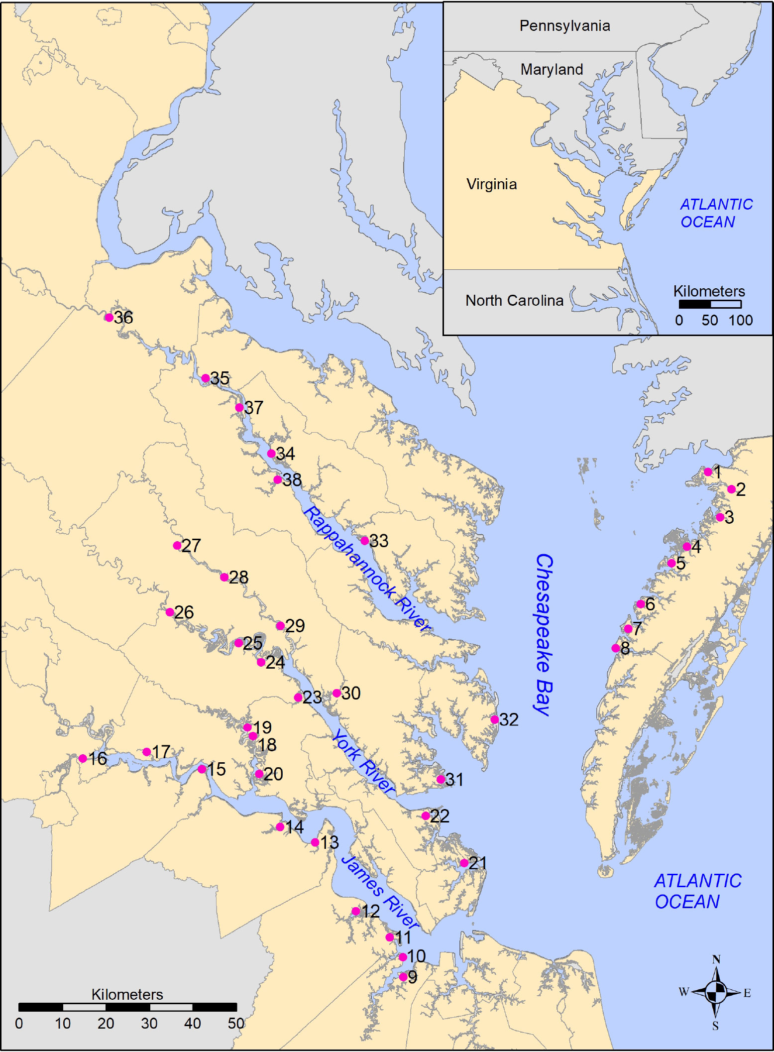
Figure 1 Reconstructed locations of marshes (sampling sites) in Edmonds et al. (1990), with inset showing relationship of study area to the Mid-Atlantic coast, USA.
2.3 Predictors of organic matter
Depth is a key correlate of organic matter content (OM). Within the marsh sediments, OM tends to decline with depth, more rapidly in the top ∼ 20 cm and less rapidly in deeper sediments as the remaining OM is more refractory (Morris and Bowden, 1986). Edmonds et al. (1990) considered three depth ranges for mineral soils: 0–13 in (∼ 0–33 cm), 13–26 in (∼ 33–66 cm), and 26–40 in (∼ 66–102 cm). (See Supplementary Material for additional information about depth ranges.) Instead of regarding depth as a categorical predictor with ordinal values of top, mid, and bottom, we take depth as a numerical predictor by taking approximate middle values of the mineral soil ranges in inches, namely, 6, 19, and 33. Employing an explicitly numerical predictor simplifies the regression model structure, in the presence of various other multilevel categorical predictors.
Among the remaining predictor variables, all are categorical, and they also contain overlapping information about the marsh environment:
● Soil category (5 levels, Figure 2A): Edmonds et al. (1990) describe 6 soil categories, namely, Fluvaquent, Hydraquent, Sulfaquent, Sulfihemist, Hydraquentic Humaquept, and Histic Humaquept. Since the Humaquepts are the only categories with modifiers and there is only one of each, we omit those from the full set of 38 marshes in the sample in order to preserve statistical power, leaving a reduced set of 36 marshes.
● Soil type (12 levels, Figure 2B), as given in Edmonds et al. (1990): In soil surveys, these are formally known as soil components and tend to be locality specific. As such, it is difficult to compare them across the spatial extent of the study.
● Vegetation type (7 levels, Figure 2C), as given in Edmonds et al. (1990): Arrow Arum-PickerelWeed (APW), Big CordGrass (BCG), Black NeedleRush (BNR), Brackish Water Mixed (BWM), Freshwater Mixed Community (FMC), Saltmarsh CordGrass (SCG), and SaltMeadow Combined (SMC).
● Inundation (3 levels, Figure 2D) and Salinity (2 levels, Figure 2E): Tidal marsh vegetation is directly controlled by inundation level and salinity of the environment (Anderson et al., 2022), with particular species or communities in saline, brackish, and freshwater areas, and subsets of those communities at different elevations within the tide range. Therefore, estimated salinity and period of inundation can be inferred from the plant community. In addition, spatially explicit salinity datasets (based on the Chesapeake Bay Program’s salinity assignments, as described in Mitchell et al., 2020) were used to help characterize local conditions into 2 levels of salinity (salt, fresh). For inundation, we initially connected the vegetative communities as described in Edmonds et al. (1990) to 3 levels (low, mid, high). Because the distribution of marsh plants are highly regulated by the frequency of inundation, we assigned low inundation to reflect a community dominated by high marsh plants, and high inundation, a community dominated by low marsh plants. The mid inundation category encompassed sites where the vegetation was evenly mixed between high and low marsh plants. However, preliminary analyses using the 3-level categorization identified the unnecessary breakdown between mid and low inundation (Longo, 2022). Therefore, in this paper we combine them as a single not-high (= low/mid) category.
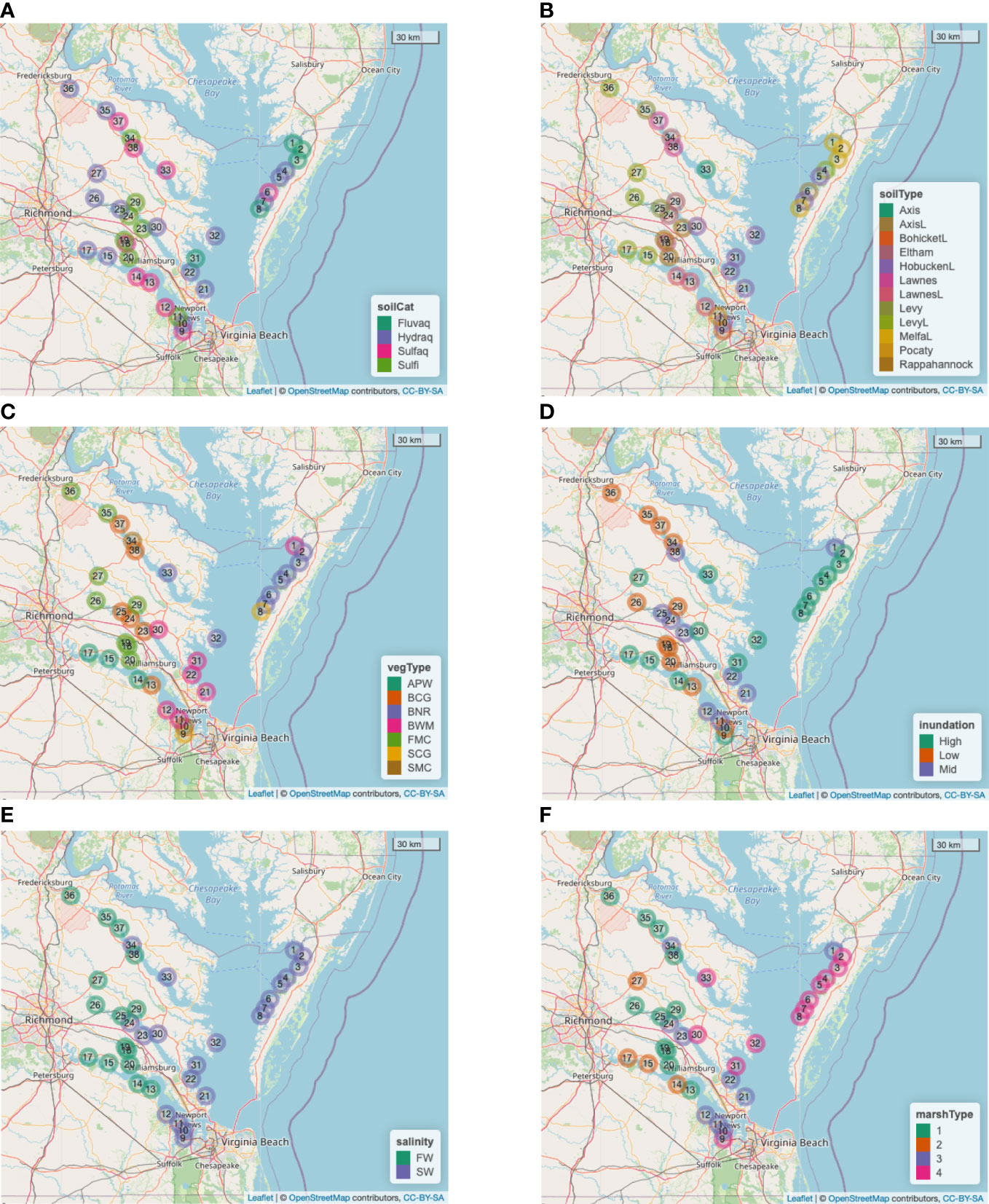
Figure 2 Spatial distributions of categorical variables across the 36 marshes considered for modeling (i.e., excluding Sites 16 and 28). (A) Soil category (Fluvaquents, Hydraquents, Sulfaquents, Sulfihemists). (B) Soil type (“L” at the end of a category denotes “loam”). (C) Vegetation type. (D) Inundation. (E) Salinity (Freshwater, Saltwater). (F) Newly defined Marsh type by crossing Inundation with Salinity (‘1’=Low/Mid–FW, ‘2’=High–FW, ‘3’=Low/Mid–SW, and ‘4’=High–SW).
The large number of categorical predictors relative to the number of marshes poses a challenge to modeling. For a regression model, each categorical predictor contributes a number of unknown model parameters that is no fewer than the number of levels minus one; this base number increases multiplicatively if interactions between predictors are considered. For this reason, we take the following measures to preserve statistical power:
● Omit soil type.
● Omit Sites 16 and 28, the only Humaqueptic sites under soil category.
● Replace the original vegetation type categorization with a new 4-level categorization of marsh type, defined by crossing the 2-level inundation and 2-level salinity. The resulting marsh type categories are ‘1’ = Low/Mid–FW, ‘2’ = High–FW, ‘3’ = Low/Mid–SW, and ‘4’ = High–SW (Figure 2F).
The new definition of marsh type implies collinearity between marsh type and each of inundation and salinity, so that the latter two cannot enter the regression model as predictors alongside marsh type. Therefore, the final set of regression predictors includes marsh type, depth, soil category, and marsh site.
2.4 Transformation of organic matter measurements
The dependent variable of interest is sediment core OM, recorded in g/kg of soil. For linear mixed modeling, the distribution of the dependent variable should not exhibit substantial skewness. Figure 3 shows that the distribution of these OM data are highly right-skewed, but log-transformation substantially reduces the skewness. Therefore, we model log(OM) as a response of the above predictor variables.
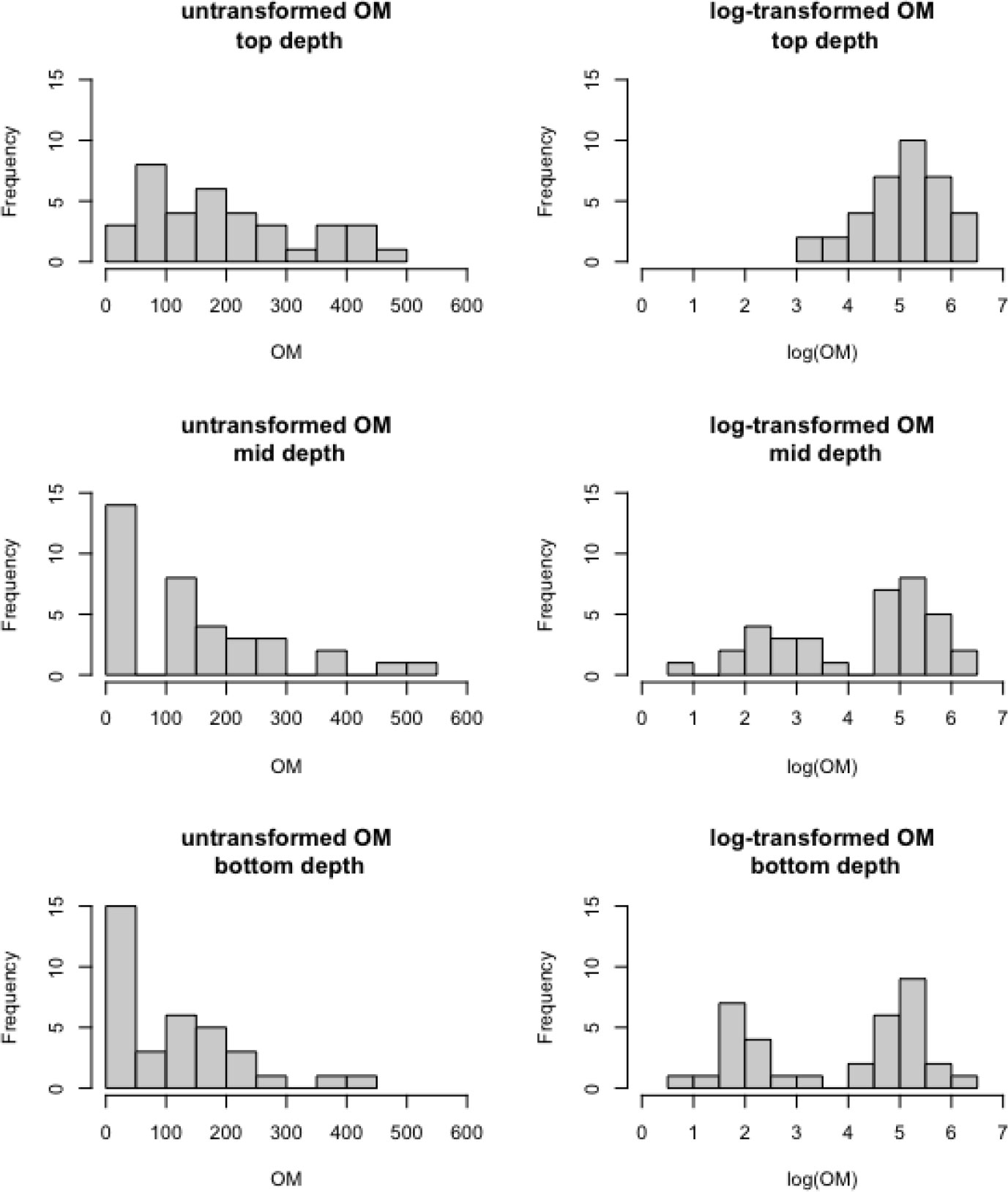
Figure 3 Distributions of sediment core organic matter in g/kg soil (left panels) and log(g/kg soil) (right panels) across the 36 marshes observed at the top depth (top panels), middle depth (middle panels), and bottom depth (bottom panels), respectively.
3 Methods
3.1 Bayesian spatial regression modeling
Point-referenced spatial data, such as ours, are often modeled using a classical geostatistical (continuous-space) model, in which the covariance between two spatial locations is described by a proposed functional form (e.g., exponential decay) with unknown parameters (see, e.g., Zimmerman and Stein, 2010). For our data, however, the sampled marshes fall along highly irregular shorelines in the lower Chesapeake Bay. That is, the sampling universe of the study area is far from being a contiguous spatial domain, and it would be rather unreasonable to employ a modeling approach that is meant for continuous space.
An alternative is to assume a conditional autoregressive (CAR) spatial structure. CAR is a nearest-neighbor dependence structure that is typically employed to model areally aggregated data, in the form of either a lattice (i.e., a regular grid, e.g., Chiu et al., 2013), or a set of irregular polygons (e.g., Hyman et al., 2022). Two areal units are considered immediate neighbors if they share a border. CAR models with first-order dependence only consider nearest neighbors. Higher-order dependence CAR models are possible by further modeling the dependence of a site with its neighbors’ immediate neighbors (e.g., Chiu and Lehmann, 2011). For the CAR structure to model point-referenced data, the investigator must decide what constitutes a pair of neighbors. White and Ghosh (2009) developed the stochastic neighborhood CAR, or SNCAR, model for point-referenced data, while avoiding the need for an upfront definition of neighbors. The SNCAR model infers a suitable threshold distance as an unknown model parameter, whereby only those marshes located within each other’s threshold radius are considered neighbors. For neighboring marshes, the SNCAR model further assumes an exponential decay covariance.
However, the SNCAR model is highly complex; for a first attempt of spatially explicit modeling of data with potential implications for blue carbon stocks, we choose the simpler first-order intrinsic CAR, or ICAR, dependence structure (e.g., Chiu et al., 2013) with a rather arbitrary threshold. ICAR is a degenerate case of CAR, whereby the conditional spatial correlation between neighbors (given all other marshes) is fixed at 1. For the threshold radius, one extreme would be to take it as the smallest pairwise distance in the dataset, leading to the sparsest possible neighborhood structure, and containing as few as a single pair of neighbors. The other extreme would be to take the largest pairwise distance as the threshold, so that every site is a neighbor of every other site. Mathematically, a certain level of sparsity is required for model estimability; with only 36 marshes, estimating the spatial parameters alongside numerous regression coefficients is rather ambitious. As such, we construct preliminary models using a threshold radius of 16 km, 24 km, and 36 km, respectively, each of which results in a neighborhood structure that is reasonably sparse without having too few pairs of neighbors to inform the statistical inference for the spatial parameters. The preliminary results show little sensitivity to the thresholds (see Supplementary Material), and subsequently we take 24 km as the threshold for formal modeling. The resulting neighborhood structure is depicted as an adjacency matrix in Figure 4.
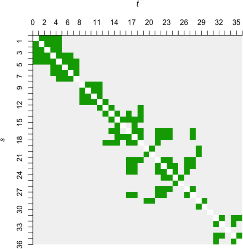
Figure 4 The adjacency matrix (symmetric) of 36 × 36 cells based on a 24 km threshold radius. Marshes s and t are considered neighbors if they are located within the threshold radius of each other, and the cell on the s -th row and t -th column of the adjacency matrix appears green. A gray cell denotes non-neighbors. White cells along the diagonal denote not applicable, as the notion of neighborhood between a marsh and itself is undefined. Note that the cell labels run from 1 to 36 (not 38) due to the omission of Sites 16 and 28.
3.2 Model statements
Our spatial regression model appears as Eqs. (1)–(3) below. It is a linear mixed model, with log-transformed OM regressed on marsh site (categorical), marsh type (categorical), soil category (categorical), depth (numerical, based on ordinal depth ranges), and the interaction between depth and marsh type; marsh site effects are modeled as random, on which the ICAR spatial autocorrelation structure is assumed. The interaction between depth and marsh type allows the slope between log(OM) and depth to differ across marsh types. We do not consider other interaction terms in the model due to either in estimability or no improvement in goodness-of-fit based on preliminary analyses (see Supplementary Material).
For the i -th marsh site (i=1,…,36 ) at the j -th depth (j=1,2,3 , except for i=11 for which j=1,2 only), let yijkℓ denote the log(OM) associated with the numerical predictor, depth, denoted by xij(=6,19,33) , and marsh type k and soil category ℓ . Note that the 107 pairs of (i,j) are nested inside k and ℓ . Further, let wij denote the standardized values of xij , i.e., the 107 values of wij 's have mean 0 and standard deviation 1 (depths are standardized to ensure numerical stability). Then, the regression model is
where β0 and β1 are the overall intercept and slope parameters with respect to depth; α1k and γℓ are the main effects (fixed effects) on yijkℓ due to marsh type k(=1,…,4) and soil category ℓ(=1,…4) , respectively; α2k is the interaction effect (fixed effect) on yijkℓ between marsh type and depth; ϕi is the spatially autocorrelated random effect due to the i -th marsh site, with variance ; and ϵijkℓ is white noise (regression error), with variance σ2 . Fixed effects are subject to the linear constraint α11=α21=γ1=0 .
For Bayesian inference, all unknown parameters (appearing only on the right-hand-side of Eqs. (1)–(3)) require prior distributions that reflect the modeler’s a priori understanding unrelated to the data at hand. Prior distributions can be inspired by historical datasets or mechanistic models. However, when an obvious source of inspiration is absent, priors that are diffuse with respect to exploratory analyses may be employed to reflect the modeler’s lack of concrete knowledge about the parameters. We take the latter approach in this paper for Eqs. (4) and (6) using relatively diffuse normal and lognormal distributions, respectively (see Supplementary Material for details):
We elaborate upon our choice of the uniform prior distribution for σϕ from Eq. (5) in Section 4.
For model comparison, we also fit the simpler mixed model whereby the random marsh site effects ϕi are assumed to be uncorrelated, i.e., Eq. 2 is replaced by ; to simplify the code, we use the same log-normal prior distribution from Eq. (6) for both σ and σϕ .
3.3 Model implementation
For exploratory modeling, we employ classical (non-Bayesian) regression that requires minimal computational effort. The specific software packages are the R functions lme4::lmer (Bates et al., 2015) and mgcv::gam (Wood, 2017) — see Supplementary Material for details. For formal modeling, we implement our Bayesian models in the Stan modeling language interfaced with the rstan package (Stan Development Team, 2022). Stan conducts Markov chain Monte Carlo (MCMC) simulations from the posterior distribution, which is the joint probability distribution of all model parameters given the observed data and stipulated model from Section 3.2. In addition to the posterior distribution on which Bayesian inference is based, MCMC simulations also facilitate a wide range of inference summaries and model diagnostics.
The posterior distribution is typically highly complex for spatially explicit models, in which case MCMC would be computationally intensive. Our code is run on a high performance computing cluster for both the ICAR and uncorrelated models. The code and output appear in Supplementary Material.
4 Results
4.1 Technical results
The uncorrelated model converges readily with very good MCMC mixing (statistical behavior of the simulated posterior draws). As anticipated, the ICAR model requires substantially more computational effort. Moreover, if the prior distribution for σϕ in Eq. (5) is replaced with one that extends to the left towards 0, such as a diffuse lognormal or uniform(0.01, 1), then the posterior distribution exhibits multimodality. While a multimodal posterior may not suggest an inherently flawed model, the model as stipulated by Eqs. (1)–(6) results in better MCMC mixing, a unimodal posterior, and some evidence of better cross-validation performance, according to the leave-one-out information criterion (LOOIC) and expected log predictive density (ELPD) via the R package loo. (Vehtari et al., 2017) (Table 1).

Table 1 LOOIC and ELPD of the ICAR and uncorrelated models.
According to Table 1, predictive performance is best for the ICAR model with a uniform(0.22, 1) prior for σϕ , followed by the same model but with a σϕ prior that extends towards 0, then by the uncorrelated model. In Subsection 4.2, we discuss the vastly different conclusions based on the best ICAR model and the uncorrelated model. Before that, first note that the difference in ELPD between the best ICAR model and the uncorrelated model is essentially the size of its SE. Thus, strictly speaking, the best and worst models (and other models in between) are rather statistically consistent with each other with respect to predictive performance. This implies that spatial autocorrelation cannot be clearly ruled out, even if the evidence is mild.
If our key objective here were to make scientific discoveries based on the statistical inference from this dataset, it might be customary to adhere to the principle of parsimony and select the least complex model that is not clearly worse in predictive performance. However, because our least and most complex models yield vastly different scientific insights, more thought must be given to the process of model selection. In fact, our needs do not lie in the statistical inference from this historical proxy dataset. Rather, the objective of our paper is to demonstrate the potential for scientific insights into blue carbon stocks at various spatial scales by employing the methodology of spatial regression modeling; the proxy data are employed here to demonstrate the methodology.
4.2 Implications of spatial ICAR vs. uncorrelated random marsh site effects
Spatial regression is a type of model-based spatial smoothing. In this case, the quantities being smoothed over space is the marsh site random effects ϕi . Figure 5 shows that the posterior median values of ϕi indeed are more spatially similar in size and in sign (positive or negative) for the ICAR model (panels A and C) than for the uncorrelated model (panels B and D). Also note that the posterior medians for the ICAR model are collectively larger with narrower Bayesian confidence intervals (CIs), implying that the marsh site effects on OM are more statistically noticeable. Importantly, there is noticeable spatial grouping of the ϕi 's — based on minimal overlapping of CIs in Figure 5C, a possible partition of the marshes into distinct groups is: {1–8} (all Eastern Shore sites), {9–15, 17–20, 23–27, 29, 30, 34–38} (all upstream sites except for sites 9–12), {21, 22, 31, 32} (all sites on the lower western shore), and {33} (the only outstanding upstream site). A finer grouping, although less statistically evident due to overlapping CIs, may be roughly defined as these sets of marshes: {1–8}, {9–12, 17, 24, 25}, {13, 14, 15, 18, 19, 20, 23, 29, 30}, {21}, {22, 31, 32}, {26, 27, 36}, {33}, and {34, 35, 37, 38}. All marshes within each set in the finer grouping — except for the two sets that include site numbers displayed in bold or italic — exhibit spatial proximity in Figure 5A. Among the four “outsider” marshes given in bold and italic, sites 24 and 25 are located next to each other.
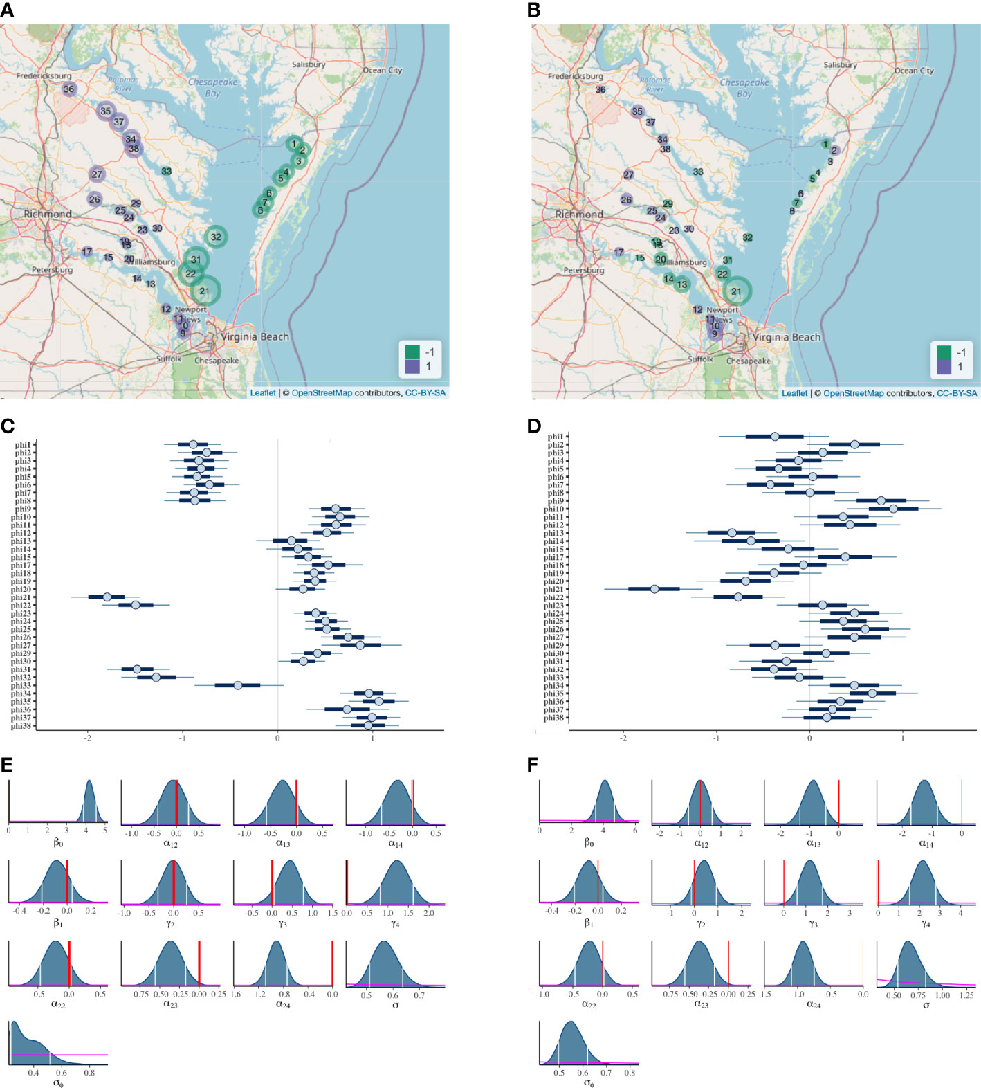
Figure 5 Bayesian inference results from the ICAR model of Eqs. (1)–(6) (panels A, C, and E) and uncorrelated model (panels B, D, and F). Panels (A, B): bubble plot of ϕi (marsh site effect), where a large purple bubble represents a highly positive value for the estimated marsh site effect (posterior median of ϕi ), and a large green bubble, a highly negative value. Panels (C, D): Bayesian confidence intervals for ϕi at confidence levels of 50% (dark blue line) and 80% (light blue line); circles denote estimated marsh site effects. Panels (E, F): marginal posterior distributions for the regression coefficients and variance parameters, with 80% confidence intervals delimited by white vertical lines, prior distributions shown in magenta, and the value 0 marked in red for the regression coefficients.
Therefore, overall, the ICAR results suggest that when spatial autocorrelation is formally modeled alongside predictor variables that have been documented to be potential drivers of blue carbon stock, a latent spatial grouping emerges, one that is not already accounted for by the predictors. This spatial phenomenon is clearly absent from the results of the uncorrelated model, as demonstrated by the lack of spatial pattern among the posterior medians in Figures 5B, D.
With respect to the predictor variables, their statistical relevance to OM is clearly demonstrated in either model (Figures 5E, F). In particular, soil category matters to OM (at least one γℓ has an 80% CI that is far from 0), and both depth and marsh type are relevant to OM at least through their interaction (the CIs for two of three α2k ’s are far from 0), even if the respective main effects may be less statistically evident (0 is inside the CI for β1 from both models, and none of the CIs for α1k ’s from the ICAR model is far from 0).
Finally, in Figures 5E, F, the non-restrictive nature of our prior distributions is evidenced by their flatness, contrasted with the peakedness of the marginal posterior distributions of the individual parameters. In other words, the statistical inference is heavily dominated by the information contributed by the data and minimally by our rather arbitrary choice of the prior distributions.
5 Discussion
The statistical model-based analysis in this paper shows that the inclusion of geospatial considerations when examining differences in tidal marsh OM stocks can result in a markedly different scientific interpretation of variability across marshes. This results in important implications for making inference of blue carbon stocks when it is based only on a few localized samples but extrapolated to unsampled areas. There is an increasing interest in estimating blue carbon stocks both for global climate models and for economic valuation, such as the growing blue carbon market (e.g., van den Bergh and Botzen, 2015). Enhancement of blue carbon stocks is a targeted activity for mitigating climate change (Trumper et al., 2009) but practical implementation of this activity requires a sophisticated understanding of blue carbon stocks and sequestration rates. Macreadie et al. (2019) called out the importance of reducing uncertainties about blue carbon stocks as critical for proper valuation of the resources and the calculation of carbon dioxide emission offsets. The actual number of carbon cores that can be used to infer this information, however, is geospatially limited, and its spatial variability is generally unknown. This has led to a tendency to use a single value for blue carbon sequestration rates and stocks across all marshes (e.g., Chmura et al., 2003; Duarte et al., 2013; Howard et al., 2014). This approach is recognized as limiting inference of carbon stocks due to the high spatial variability in marsh carbon content, but is a necessary approach where data are limited (Lawrence et al., 2012; Ewers Lewis et al., 2018). Our model-based analysis suggests that, while the use of a single average number may be appropriate in some circumstances, it may be dramatically incorrect in others.
Specifically, in the case of the historical OM data, when geospatial considerations are incorporated (Figure 5C), it is clear that marsh site effects tend to have tighter confidence intervals and their estimates (posterior medians) tend to be much closer to adjacent marshes than marshes further away. The similarity between adjacent marshes is interesting, since (i) it suggests that there are some location-specific marsh characteristics beyond marsh type, depth, or soil category that are affecting OM stocks, and (ii) a single average value of log(OM) would be a grossly inappropriate representation of tidal marsh OM content across the study region, masking the distinction among group averages as revealed by the spatially explicit model. It has been previously shown that autochthonous OM sources such as marsh vegetation are an important control on stocks (since different marsh plants have different levels of productivity, persistence, and recalcitrance; see Ewers Lewis et al., 2020) and our model results support those findings (α2k ’s in Figures 5E, F). The geospatial analysis suggests that OM content of allochthonous sediment contribution maybe equally important to the stock within a given marsh. For example, Figure 5C shows that sites 21, 22, 31, and 32 are less tightly grouped than sites 1–8, although site 32 shares a vegetative community with sites 2–6. Because sites 21, 22, 31, and 32 are facing the mouth of the Chesapeake Bay, they are susceptible to sediment erosion and sand overwash during high energy wave events. This may reduce the retention of autochthonous OM and add allochthonous mineral sediment to the marshes, and could be the reason for site 32 to be distinguishable from 2–6.
In contrast, when geospatial considerations are excluded from the statistical model, groupings between marshes are limited: the values of the estimated marsh site effects are distributed broadly, with confidence intervals that are wider and tend to overlap (Figure 5D). That is, based on the more simplistic uncorrelated model, spatial variability is substantial even after adjusting for the predictor variables marsh type, depth, and soil category. This large variability suggests that a single average value of log(OM) — given a specific combination of marsh type, soil category, and soil depth — might be a justified representation across the entire Chesapeake Bay, if the scientific purpose was to estimate the region’s OM stock for use in a climate model, for example. However, based on the widely variable values of the estimated marsh site effect, it is clear that a single number does not represent any given marsh particularly well (Figure 5D). Thus, when the purpose is to estimate the OM content of any particular marsh, the single-value approach could lead to valuable loss of site-specific information about OM stocks. This reasoning also highlights the importance of the distribution of sampling sites for different inference purposes. For large-scale OM estimation, it is clearly important for the sampling sites to be relatively evenly spaced across the spatial region of inference to allow adequate interpolation of OM stocks. For example, according to our geospatial analysis, using data from the Rappahannock River could provide a biased estimate of OM stocks in the upper James River, despite the similarity in salinity distribution and marsh plant vegetation. However, for estimation of OM stocks in a particular marsh — for example, an unsampled marsh on the lower James — samples that are clustered around the marsh of interest may be required.
Note that within a tidal marsh, both plant composition and hydrologic regimes tend to be stable over annual to decadal time frames. Also, although upland soil organic carbon can vary temporally with changes in land use (e.g., Ma et al., 2018), it tends not to when land use is consistent over sampling periods (López-Teloxa et al., 2017). Therefore, our models have not considered temporal variation. In contrast, the tidal marsh OM dataset featured in our paper has allowed us to explore the importance of geospatial consideration in the potential future modeling of blue carbon stocks, because carbon stock datasets with broad geospatial representation and consistent sampling techniques across space are rare to date. We anticipate that our approach and implications discussed above regarding OM will be directly applicable to carbon stock modeling, due to the high correlation between tidal marsh OM and total organic carbon (TOC; Craft et al., 1991). Because TOC values are almost always much lower than OM values (e.g., 4% and 36%, respectively), a rigorous geospatial modeling approach that can discern subtle changes may prove to be especially important. We anticipate applying the statistical methodology of this paper to new TOC data (currently being collated) from an extensive sampling effort of CBVA marshes which was conducted in November 2021 as part of a collaborative grant with the US National Resources Conservation Service. Our methodology should result in improved insights into blue carbon stocks compared to conventional approaches for extrapolating known blue carbon stocks to unsampled marshes.
Data availability statement
The original contributions presented in the study are included in the article/Supplementary Material. Further inquiries can be directed to the corresponding authors.
Author contributions
GC, MM, and JH conceived the research and wrote the paper. MM chose and formatted the data, reconstructed the site locations, and constructed the variables inundation and salinity. Under the guidance of GC: KD conducted graphical data exploration of a subset of the original sampling sites; CL formalized these exploratory results by building and implementing an ICAR model for the same subset. GC extended the model by CL to accommodate the 36 sites of this paper, including model implementation (for all model variants in this paper) and model diagnostics. MM and JH advised on model refinement. All authors contributed to the article and approved the submitted version.
Funding
FO USDA-NRCS-NHQ-SOIL-20-NOFO0001003, 2020 Soil Science Collaborative Research Proposals Award # NR203A750025C010.
Acknowledgments
The authors acknowledge William & Mary Research Computing for providing computational resources and technical support that have contributed to the results reported within this paper (URL: https://www.wm.edu/it/rc). We thank the two reviewers for their valuable input. We also thank C. Friedrichs (VIMS) for suggesting this Special Topic as a publication outlet for our research.
Conflict of interest
The authors declare that the research was conducted in the absence of any commercial or financial relationships that could be construed as a potential conflict of interest.
Publisher’s note
All claims expressed in this article are solely those of the authors and do not necessarily represent those of their affiliated organizations, or those of the publisher, the editors and the reviewers. Any product that may be evaluated in this article, or claim that may be made by its manufacturer, is not guaranteed or endorsed by the publisher.
Supplementary material
The Supplementary Material for this article can be found online at: https://www.frontiersin.org/articles/10.3389/fmars.2022.1056404/full#supplementary-material
References
Anderson S. M., Ury E. A., Taillie P. J., Ungberg E. A., Moorman C. E., Poulter B., et al. (2022). Salinity thresholds for understory plants in coastal wetlands. Plant Ecol. 223, 323–337. doi: 10.1007/s11258-021-01209-2
Bates D., Mächler M., Bolker B., Walker S. (2015). Fitting linear mixed-effects models using lme4. J. Stat. Software 67, 1–48. doi: 10.18637/jss.v067.i01
CCRM (2017). Comprehensive coastal inventory program Gloucester Point, Virginia: Center for Coastal Resources Management (CCRM) Digital Tidal Marsh Inventory Series, Virginia Institute of Marine Science.
Chiu G. S., Lehmann E. A. (2011). “Bayesian Hierarchical modelling: incorporating spatial information in water resources assessment and accounting,” in MODSIM2011, 19th International Congress on Modelling and Simulation, Perth, Australia. 3349–3355.
Chiu G. S., Lehmann E. A., Bowden J. C. (2013). A spatial modelling approach for the blending and error characterization of remotely sensed soil moisture products. J. Environ. Stat 4(9). Available at: http://www.jenvstat.org/v04/i09.
Chmura G. L. (2009). “Tidal salt marshes,” in The management of natural coastal carbon sinks. Eds. Laffoley D.d’A., Grimsditch G. Gland, Switzerland:International Union for Conservation of Nature and Natural Resources (IUCN).
Chmura G. L., Anisfeld S. C., Cahoon D. R., Lynch J. C. (2003). Global carbon sequestration in tidal, saline wetland soils. Global Biogeochemical Cycles 17. doi: 10.1029/2002GB001917
Connor R. F., Chmura G. L., Beecher C. B. (2001). Carbon accumulation in bay of fundy salt marshes: Implications for restoration of reclaimed marshes. Global Biogeochemical Cycles 15, 943–954. doi: 10.1029/2000GB001346
Coverdale T. C., Brisson C. P., Young E. W., Yin S. F., Donnelly J. P., Bertness M. D. (2014). Indirect human impacts reverse centuries of carbon sequestration and salt marsh accretion. PloS One 9, e93296. doi: 10.1371/journal.pone.0093296
Craft C. (2007). Freshwater input structures soil properties, vertical accretion, and nutrient accumulation of Georgia and U.S tidal marshes. Limnol. Oceanogr. 52, 1220–1230. doi: 10.4319/lo.2007.52.3.1220
Craft C. B., Seneca E. D., Broome S. W. (1991). Loss on ignition and kjeldahl digestion for estimating organic carbon and total nitrogen in estuarine marsh soils: Calibration with dry combustion. Estuaries 14, 175. doi: 10.2307/1351691
Duarte C. M., Losada I. J., Hendriks I. E., Mazarrasa I., Marbà N. (2013). The role of coastal plant communities for climate change mitigation and adaptation. Nat. Climate Change 3, 961–968. doi: 10.1038/nclimate1970
Duarte C. M., Middelburg J. J., Caraco N. (2005). Major role of marine vegetation on the oceanic carbon cycle. Biogeosciences 2, 1–8. doi: 10.5194/bg-2-1-2005
Edmonds W. J., Hodges R. L., Peacock C. D. (1990). Tidewater Virginia tidal wetland soils: a reconnaissance characterization. Tech. rep. Virginia Agric. Experiment Station.
Ewers Lewis C. J., Carnell P. E., Sanderman J., Baldock J. A., Macreadie P. I. (2018). Variability and vulnerability of coastal ‘Blue carbon’ stocks: A case study from southeast Australia. Ecosystems 21, 263–279. doi: 10.1007/s10021-017-0150-z
Ewers Lewis C. J., Young M. A., Ierodiaconou D., Baldock J. A., Hawke B., Sanderman J., et al. (2020). Drivers and modelling of blue carbon stock variability in sediments of southeastern Australia. Biogeosciences 17, 2041–2059. doi: 10.5194/bg-17-2041-2020
Howard J., Hoyt S., Isensee K., Pidgeon E., Telszewski M. (2014). Coastal Blue Carbon: Methods for assessing carbon stocks and emissions factors in mangroves, tidal salt marshes, and seagrass meadows (Arlington, Virginia, USA:Conservation International, Intergovernmental Oceanographic Commission of UNESCO, International Union for Conservation of Nature (IUCN)).
Hyman A. C., Chiu G. S., Fabrizio M. C., Lipcius R. N. (2022). Spatiotemporal modeling of nursery habitat using Bayesian inference: Environmental drivers of juvenile blue crab abundance. Front. Mar. Sci. 9. doi: 10.3389/fmars.2022.834990
Lavery P. S., Mateo M.-Á., Serrano O., Rozaimi M. (2013). Variability in the carbon storage of seagrass habitats and its implications for global estimates of blue carbon ecosystem service. PloS One 8, e73748. doi: 10.1371/journal.pone.0073748
Lawrence A., Baker T., Lovelock C. (2012). Optimising and managing coastal carbon: Comparative sequestration and mitigation opportunities across australia’s landscapes and land uses: Final report TierraMar Consulting Pty Ltd., FRDC, Deakin, ACT, Australia: Prepared for the Fisheries Research and Development Corporation (FRDC).
Le N. D. (2006). “Prediction intervals, spatial,” in Encyclopedia of environmetrics. Eds. El-Shaarawi A. H., Piegorsch W. W. (Chichester, UK:Wiley). doi: 10.1002/9780470057339.vap035
Longo C. (2022). Bayesian Spatial model development of soil core organic matter as a proxy for blue carbon stocks within the Chesapeake bay (Williamsburg, Virginia:Undergraduate honors theses, William & Mary). Available at: https://scholarworks.wm.edu/honorstheses/1824.
López-Teloxa L. C., Cruz-Montalvo A., Tamaríz-Flores J. V., Pérez-Avilés R., Torres E., Castelán-Vega R. (2017). Short-temporal variation of soil organic carbon in different land use systems in the ramsar site 2027 ‘Presa Manuel Ávila camacho’ puebla. J. Earth Syst. Sci. 126, 95. doi: 10.1007/s12040-017-0881-4
Macreadie P. I., Anton A., Raven J. A., Beaumont N., Connolly R. M., Friess D. A., et al. (2019). The future of blue carbon science. Nat. Commun. 10, 3998. doi: 10.1038/s41467-019-11693-w
Ma R., Shi J., Zhang C. (2018). Spatial and temporal variation of soil organic carbon in the north China plain. Environ. Monit. Assess. 190, 357. doi: 10.1007/s10661-018-6734-z
Mcleod E., Chmura G. L., Bouillon S., Salm R., Björk M., Duarte C. M., et al. (2011). A blueprint for blue carbon: toward an improved understanding of the role of vegetated coastal habitats in sequestering CO 2. Front. Ecol. Environ. 9, 552–560. doi: 10.1890/110004
McTigue N., Davis J., Rodriguez A. B., McKee B., Atencio A., Currin C. (2019). Sea Level rise explains changing carbon accumulation rates in a salt marsh over the past two millennia. J. Geophys. Res.: Biogeosci. 124, 2945–2957. doi: 10.1029/2019JG005207
Mitchell M. (2018). Impacts of Sea level rise on tidal wetland extent and distribution Gloucester Point, Virginia: Dissertations, theses, and masters projects, William & Mary. doi: 10.25773/v5-5s6z-v827
Mitchell M., Herman J., Hershner C. (2020). Evolution of tidal marsh distribution under accelerating Sea level rise. Wetlands 40, 1789–1800. doi: 10.1007/s13157-020-01387-1
Morris J. T., Bowden W. B. (1986). A mechanistic, numerical model of sedimentation, mineralization, and decomposition for marsh sediments. Soil Sci. Soc. America J. 50, 96–105. doi: 10.2136/sssaj1986.03615995005000010019x
Stan Development Team (2022) RStan: the R interface to Stan. R package version 2.21.5. Available at: https://mc-stan.org/rstan.
Sullivan M. J., Currin C. A. (2002). “Community structure and functional dynamics of benthic microalgae in salt marshes,” in Concepts and controversies in tidal marsh ecology (Dordrecht: Kluwer Academic Publishers), 81–106. doi: 10.1007/0-306-47534-06Sullivan2002
Trumper K., Bertzky M., Dickson B., van der Heijden G., Jenkins M., Manning P. (2009). The natural fix? the role of ecosystems in climate mitigation: A UNEP rapid response assessment (Cambridge, UK:United Nations Environment Programme).
van den Bergh J., Botzen W. (2015). Monetary valuation of the social cost of CO2 emissions: A critical survey. Ecol. Economics 114, 33–46. doi: 10.1016/j.ecolecon.2015.03.015
Vehtari A., Gelman A., Gabry J. (2017). Practical Bayesian model evaluation using leave-one-out cross-validation and WAIC. Stat Computing 27, 1413–1432. doi: 10.1007/s11222-016-9696-4
White G., Ghosh S. K. (2009). A stochastic neighborhood conditional autoregressive model for spatial data. Comput. Stat Data Anal. 53, 3033–3046. doi: 10.1016/j.csda.2008.08.010
Wood S. (2017). Generalized additive models: An introduction with R. 2 edn (New York, New York:Chapman and Hall/CRC).
Keywords: blue carbon, coastal sediment, spatial regression, conditional autoregressive dependence, Markov random field (MRF), Bayesian modeling and inference
Citation: Chiu GS, Mitchell M, Herman J, Longo C and Davis K (2023) Enhancing assessments of blue carbon stocks in marsh soils using Bayesian mixed-effects modeling with spatial autocorrelation — proof of concept using proxy data. Front. Mar. Sci. 9:1056404. doi: 10.3389/fmars.2022.1056404
Received: 28 September 2022; Accepted: 12 December 2022;
Published: 12 January 2023.
Edited by:
Zhenhong Du, Zhejiang University, ChinaReviewed by:
Junhong Bai, Beijing Normal University, ChinaPatrick Biber, University of Southern Mississippi, United States
Copyright © 2023 Chiu, Mitchell, Herman, Longo and Davis. This is an open-access article distributed under the terms of the Creative Commons Attribution License (CC BY). The use, distribution or reproduction in other forums is permitted, provided the original author(s) and the copyright owner(s) are credited and that the original publication in this journal is cited, in accordance with accepted academic practice. No use, distribution or reproduction is permitted which does not comply with these terms.
*Correspondence: Grace S. Chiu, Z3NjaGl1QHZpbXMuZWR1; Molly Mitchell, bW9sbHlAdmltcy5lZHU=; Julie Herman, aGVybWFuQHZpbXMuZWR1