Evaluating future climate change exposure of marine habitat in the South East Pacific based on metabolic constraints

Introduction: On-going climate change is now recognized to yield physiological stresses on marine species, with potentially detrimental effects on ecosystems. Here, we evaluate the prospect of using climate velocities (CV) of the metabolic index (Φ) for assessing changes in habitat in the South East Pacific.

Methods: Our approach is based on a species with mean ecophysiotype (i.e. model species) and the use of a global Earth System Model simulation (CESM-LE) under RCP 8.5 scenario. The SEP is chosen as a case study as it hosts an Oxygen Minimum Zone and seamounts systems sustaining local communities through artisanal fisheries.

Results and Discussion: Our results indicate that CV_Φ pattern is mainly constrained by the oxygen distribution and that its sign is affected by contrasting oxygen trends (including a re-oxygenation in the upper OMZ) and warming. We further show that CV_Φ is weakly dependent on physiological traits composing Φ, which conveys to this metrics some value for inferring the projected mean displacement and potential changes in viability of metabolic habitat in a region where physiological data are scarce. Based on sensitivity experiments to physiological traits and natural variability, we propose a general method for inferring broad areas of climate change exposure regardless of species-specific Φ. We show in particular that for the model used here, the upper OMZ region can be considered a “safe” area for the species with ecophysiotype close to that of 71 species used to derive the model species. Limitations of the approach and perspectives of this work are also discussed.

1. Introduction

With climate change, marine species face the combined effect of multiple threats: warming, acidification and oxygen decline (Levin, 2018; Sampaio et al., 2021). Marine deoxygenation may be the most threatening of all stressors to marine life and has important detrimental consequences on marine ecosystems (Sampaio et al., 2021), particularly in the highly productive Eastern Boundary Upwelling Systems that host extended oxygen minimum zones (OMZ) (Garçon et al., 2019).

The South East Pacific (SEP) hosts one of the largest OMZ resulting from the weak ventilation of thermocline waters combined with the relatively high rate of microbial decomposition of organic matter (Karstensen et al., 2008; Paulmier and Ruiz-Pino, 2009; Oschlies, 2018; Pitcher et al., 2021). Despite the current deoxygenation trend at global scale (e.g., Keeling et al., 2010; Bopp et al., 2013; Schmidtko et al., 2017; Oschlies, 2018), whether or not the SEP OMZ will expand or shrink remains uncertain. On the one hand, there is still currently a low consensus amongst the latest generation of the Global Earth System Models on the future trajectory of deoxygenation rate in the SEP (Bopp et al., 2013; Cabré et al., 2015) while available observations indicate regional discrepancies in the sign of the trend (Stramma et al., 2008; Graco et al., 2017; Ito et al., 2017). On the other hand, climate projections agree on significant warming along the western coast of South America with a pattern resembling the culminating phase of a strong El Niño event (Cai et al., 2021; Dewitte et al., 2021). Increased surface temperature yields an increased vertical stratification, a phenomenon already observed (Liao et al., 2021). Increased stratification not only alters ocean dynamics in a number of ways, and thus indirectly marine ecosystems, but it has also the potential to modify directly marine habitat through modulating thermal niches (Santana-Falcón and Séférian, 2022).

As a matter of fact, shifts in species distribution have already been observed (Perry et al., 2005; Pinsky et al., 2013; Poloczanska et al., 2016) or projected (Cheung et al., 2009; Clarke et al., 2021a) as a result of habitat compression due to increasing temperature. Such changes can be captured by so-called climate velocities, a metrics that encapsulate both changes in space and time of a particular variable. Climate velocities are defined as the ratio of the long-term trend over the mean spatial gradient of a variable (Loarie et al., 2009). Previous oceanic studies have focused on temperature and showed a close relationship between species migration and speed of isotherm migrations (Burrows et al., 2014; Brito-Morales et al., 2020; Jorda et al., 2020; Thorne and Nye, 2021).

However, for marine organisms, empirical data indicate that tolerance to hypoxia decreases with increasing temperature (Pörtner and Knust, 2007). This relationship can be modeled as the ratio of temperature dependent oxygen supply to animal oxygen demand rates. This ratio termed the metabolic index Φ (Deutsch et al., 2015) is a measure of aerobic scope in an oxygen-limited environment. It describes the capability of an environment to sustain aerobic metabolic activity relative to that at rest, and thus accounts for the non-linear interaction between thermal and oxygen stresses on a particular organism. Studies using the metabolic index highlighted a close match between the metabolic index and marine species distributions (Deutsch et al., 2015; Penn et al., 2018; Deutsch et al., 2020; Howard et al., 2020). In fact, the ratio necessary to sustain active aerobic metabolism defines an ecological trait Φ_crit which has been found to correspond to the geographical limit of observed viable habitat (Deutsch et al., 2015). Below the threshold Φ_crit, species are unable to perform active aerobic metabolism. This is of particular relevance in the SEP OMZ where marine species can undergo both types of stressors (warming and hypoxia) when the OMZ limits experience changes under environmental forcing, whether they originate from natural variability (e.g. El Niño/La Niña) or from anthropogenic activities.

The SEP and its OMZ harbor a great number of species, many of them endemic (Clark et al., 2010; Friedlander et al., 2016), located in the vicinity of the OMZ upper limit along the continental slope or in the off-shore ocean where a chain of seamounts system stands along the Nazca, Salas y Gómez, and Juan Fernández ridges (Mecho et al., 2021; Tapia-Guerra et al., 2021). Although the OMZ hosts species that tolerate low oxygen conditions, it is also visited by species performing Diel Vertical Migrations (DVM), such as zooplankton (Wishner et al., 2008; Wishner et al., 2020), seeking punctual refugia from predators, or accumulating at the lower OMZ borders in micro-aerobic conditions attracted by the preserved organic matter sinking out of the OMZ (Paulmier et al., 2021). A great number of seamounts also shelters target species for artisanal fisheries (e.g., the golden crab, the Juan Fernandez lobster and the Juan Fernandez morwong (Arana and Ziller, 1985; Ernst et al., 2013; Friedlander and Gaymer, 2021) being the economic support of local communities. Artisanal fisheries supporting local Chilean and Peruvian economies (Gutiérrez et al., 2016) are also highly vulnerable to climate variability at interannual (e.g. El Niño, Carstensen et al., 2010) and decadal timescales (Bertrand et al., 2011). It is therefore useful to design resource management and adaptation strategies that account for organism responses to multiple stressors present in the SEP.

In this context, we propose to investigate future marine habitat change in the SEP (horizon 2100) from a modelling perspective applying climate velocity to the metabolic index (CV_Φ). Considering the scarcity of data to estimate physiological and ecological traits of species inhabiting the SEP (see Deutsch et al., 2015; Deutsch et al., 2020), our approach is to first explore the changes in metabolic index of a model species given climate change patterns for temperature and oxygen derived from an Earth System Model (Community Earth System Model Large Ensemble-Project). Secondly, we apply climate velocity (Loarie et al., 2009) to the metabolic index to infer future marine habitat change in the SEP, which, from a methodological point of view, expands former studies (Thorne and Nye, 2021; English et al., 2022) in a multi-factorial environmental stress (i.e. warming and oxygen changes) and for a variable (Φ) that considers species’ physiology. We show in particular that CV_Φ conveys useful pieces of information to define potential marine metabolic habitat changes, providing in particular an overview on how broad metabolic habitats would evolve in space and time under climate change for a large range of species. Our goal is also to assess the relative sensitivities of climate velocities of the metabolic index to temperature and oxygen changes (e.g. differential climate sensitivity), considering current uncertainties in the trajectory of the SEP OMZ in the warmer climate (Oschlies, 2018), in order to explore where changes in habitat are more likely to be temperature or oxygen-driven. While most results are based on a model marine species with a mean ecophysiotype, we contrast them with those of a real species for which sufficient information is available to derive the metabolic index, the shrimp Oplophorus spinosus inhabiting oxygenated waters. Along with the results and sensitivity tests to values of the physiological traits, these are used as material for discussing implications of our work.

The paper is structured as follow: Section 2 provides an overview of the dataset and methodology. Section 3 is devoted to the analysis and interpretation of climate velocities of the metabolic index and analysis on the representativeness of the results considering sensitivity analyses of climate velocities to physiological traits and uncertainties due to natural variability. Section 4 is the discussion section where we provide an assessment of exposure to climate change of broad areas based on climate velocities for species inhabiting the SEP in the horizon 2100 and discuss the limits of our approach. This section finally includes concluding remarks and perspectives.

2. Dataset and methods

2.1. Model data

In order to diagnose the climate change patterns in the SEP (Figure S1), we use the long-term simulations of the NCAR Community Earth System Model Large Ensemble Project (CESM-LE) (Kay et al., 2015; Lovenduski et al., 2016), which is derived from the Community Earth System Model, version1, with the Community Atmosphere Model, version5 (CESM1(CAM5); (Hurrell et al., 2013). Although presenting classical biases of current generation global climate models, in particular a warm bias in the eastern tropical Pacific, CESM reasonably simulates the tropical variability, including ENSO (Deser et al., 2012; Karamperidou et al., 2017; Dewitte and Takahashi, 2019) and some key aspects of the sensitivity of the carbon cycle to climate variability (Long et al., 2013). While CESM tends to overestimate the volume and spatial extent of the OMZs in the tropical Pacific (Moore et al., 2013), it properly captures the large-scale spatial pattern distribution of dissolved oxygen (Long et al., 2016) and exhibits the closest match to observations in the tropical Pacific across models (Cabré et al., 2015). Although this model simulates a negative trend in the global inventory of oxygen over the period 2006-2100 consistently with other models participating to the Climate Model Intercomparison Project (Phase 6) (Kwiatkowski et al., 2020), it predicts a positive trend in O₂ in the OMZ (Figures 1A, B, see also Figure S2 for an estimate of errors due to natural variability), which could be due to enhanced downward mixing of upper oxygenated waters in a warmer climate associated to intensified tropical variability (Carréric et al., 2020) in spite of the increased thermal stratification. Note that a few models participating to the Climate Model Intercomparison Project (Phase 6) also simulate such a positive tendency although disagreeing on its magnitude. Regarding temperature trends (Figures 1C, D), CESM is rather consistent with the ensemble mean of models participating to CMIP6 (Karamperidou et al., 2017; Cai et al., 2021). Besides its overall realism, this model resource is also perfectly suited for assessing uncertainties associated to natural variability (Figure S2), given that it provides simulations that solely differ in terms of initial conditions, thus accounting for fluctuations that originate from the internal dynamics of the earth system (Kay et al., 2015). We used temperature, salinity and oxygen outputs of the 34 members (i.e. simulations with unique initial conditions) covering the period 2006-2100 corresponding to the RCP 8.5 scenario. The oceanic model is the Parallel Ocean Program (POP, Smith et al., 2010) with a grid resolution of 1°x1° and 60 vertical layers. Hereafter, we systematically calculate the ensemble mean of specific quantities (Φ and CV_Φ, see below) using oxygen, temperature and salinity data for each of the 34 runs for two different mean climate conditions taken as “present” (2006-2036) and “future” (2070-2100) conditions.

FIGURE 1

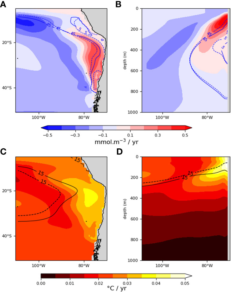
Figure 1 Ensemble mean of oxygen and temperature trends between 2006 and 2100. At 200m (A, C) and 26°S (B, D). For oxygen (top panels), the blue lines represent the projected oxygen isocontours (5 and 45 mmol.m^-3) for the “present” (mean 2006-2036, dashed) and “future” climates (mean 2070-2100, solid). For temperature trends (bottom panels), the black lines represent the projected temperature isocontours (15°C) for present (dashed) and future (plain) climates.

2.2. Metabolic index Ф

The metabolic index is a measure of aerobic scope in an oxygen-limited environment. Following (Deutsch et al., 2015; Deutsch et al., 2020), the metabolic index Φ (non-dimensional) is calculated as the ratio of O₂ (pO₂ in atm, Figure S3) supplied by the environment to the oxygen demand of an organism at rest, thus representing the coupled effect of oxygen and temperature on metabolic supply and demand (eq. 1 and 2; Deutsch et al., 2020):

$\begin{array}{ll}\begin{array}{c}\Phi =\frac{{\text{O}}_2\text{supply}}{{\text{O}}_2\text{demand}}=\frac{{\text{α}}_{\text{S}}}{{\text{α}}_{\text{D}}}{ }^{\text{Bϵ}}\text{p}{\text{O}}_2{\text{e}}^{\frac{{\text{E}}_0}{{\text{k}}_{\text{B}}}\left(\frac{1}{\text{T}}-\frac{1}{{\text{T}}_{\text{ref}}}\right)}\end{array}& (1)\end{array}$

Eq. 1 is simplified as:

$\begin{array}{ll}\begin{array}{c}\Phi ={\text{A}}_0\text{p}{\text{O}}_2{\text{e}}^{\frac{{\text{E}}_0}{{\text{k}}_{\text{B}}}\left(\frac{1}{\text{T}}-\frac{1}{{\text{T}}_{\text{ref}}}\right)}\ge {\text{Φ}}_{\text{crit}}\end{array}& (2)\end{array}$

where kB is the Boltzman constant and A₀ and E₀ the physiological traits of a given species (see Table 1). α_D and α_S are the resting metabolic rate and the efficacy of O₂ supply per unit of body mass (B) respectively. $A_0=\frac{{\alpha }_S}{{\alpha }_D}$, represents the hypoxic threshold so that 1/A₀ is the minimum oxygen that can sustain metabolic activity at rest at a reference temperature T_ref of 15°C (Penn et al., 2018; Penn and Deutsch, 2022). E₀=E_D-E_S and represents the difference between the sensitivity to temperature of oxygen demand (E_D) and oxygen supply (E_S). ϵ is the allometric scaling of the supply to demand ratio. B^ϵ is assumed equal to 1 (Penn et al., 2018; Deutsch et al., 2020; Penn and Deutsch, 2022). Below Φ = 1, oxygen demand exceeds oxygen supply capacity and organisms must suppress aerobic metabolic activities. Species must live in an environment capable of sustaining ecological activities, which is when Φ is superior to a threshold Φ_crit. Φ_crit is an ecological threshold as it represents the minimum energy requirements to support ecological activities such as swimming and feeding. In other terms, it is the threshold to maintain a population and as such, delimits geographical viable habitat. A₀, E₀ and Φ_crit define an ecophysiotype unique to each species.

TABLE 1

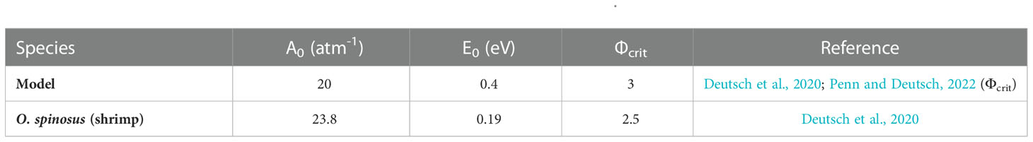
Table 1 Physiological traits (A₀ and E₀) and Ф_crit of the model species and O. spinosus.

From the most updated database (Deutsch et al., 2020), out of 71 species documented, we found estimates of A₀, E₀ and Φ_crit for only 6 species present in the SEP: 2 cephalopods (Dosidicus gigas and Octopus vulgaris) and 4 crustacea (Gaussia princeps, Notostomus elegans, Oplophorus gracilirostris and Oplophorus spinosus). As this represents a limited sample, following Penn and Deutsch (2022), we use a mean ecophysiotype: A₀ = 20 atm^-1, E₀ = 0.4 eV and Φ_crit = 3 that is representative of a model species with mean traits of real species populating regions not necessarily in the SEP. A₀ and E₀ are the mean values of physiological traits estimated for 71 species (62 for Φ_crit), benthic and pelagic, of 5 phyla (Annelida, Arthropoda, Chordata, Mollusca, and Cnidaria) in diverse ocean basins and biomes (Deutsch et al., 2020). In addition, we computed Φ for the shrimp, Oplophorus spinosus (A₀ = 23.8 atm^-1, E₀ = 0.19 eV, Φ_crit = 2.5). Metabolic traits for the shrimp were measured from animals off Hawaii (see database in Deutsch et al. (2020)) residing along a depth range of 140-750m with temperatures in the range 5-24°C (Cowles et al., 1991). We assume that these traits values are valid for the shrimps of the SEP as both environments are comparable over such a depth range. Lastly, this shrimp is found in oxygenated waters and near oxygen minimum layers and therefore may be used to represent how normoxic species may be impacted by warming and deoxygenation. Thus, we argue that the case of the shrimp can be used as a benchmark for comparing with the results obtained with the model species.

2.3. Climate velocities

2.3.1. Definition

Climate velocities describe the speed and direction at which local climate conditions are changing (Loarie et al., 2009). Climate velocities (CV, km.yr^-1) were calculated using the gradient based approach (eq. 3 and Supplementary Material eq. 3):

$\begin{array}{ll}\begin{array}{c}{\text{CV}}_{\text{Φ}}\left(\text{km}.{\text{yr}}^{-1}\right)=\frac{\text{temporal trends }\left(\text{Φ}.{\text{yr}}^{-1}\right)}{\text{spatial gradient }\left(\text{Φ}.{\text{km}}^{-1}\right)}\end{array}& (3)\end{array}$

The temporal gradient (Φ.yr^-1) represents the local rate of change and corresponds here to the 2006-2100 local linear trend for Φ in every cell (i,j). The mean spatial gradient of Φ is calculated as the square root of the sum of the squared latitudinal and longitudinal gradients of Φ. The spatial gradients (Φ.km^-1) were calculated using the same numerical scheme as that of the model code (Smith et al., 2010) so as to avoid artifacts associated to interpolation procedures. The spatial gradient indicates the difference in local conditions between adjacent cells. It is always positive and the direction of the gradient can be inferred from the angle between the latitudinal and longitudinal gradients. Climate velocities therefore represent the rate of change modulated by the spatial distribution of the climate variable. Hence, climate velocities of the Metabolic Index (CV_Φ) indicate where (direction) and how fast (speed) the local and present metabolic index (Φ in 2006 in any cell (i, j)) is projected to displace by 2100. For example, if the metabolic index decreases (negative velocities) at some location, the species would need to move in the direction of increasing Ф, that is in the direction of the gradient. Therefore, CV_Φ indicates where species would migrate (Brito-Morales et al., 2018) in 2100 if they were tracking their present metabolic index (Φ in 2006). In practice, there are many instances when the value of Φ of some species is sufficiently larger than the value of Φ_crit so that these species may not be sensitive to CV_Φ. However CV_Φ still informs on the distance between Φ and Φ_crit in the future climate, which conveys information on the extent of the changes in metabolic habitat for that particular species independently of whether it migrates or not. In addition, since Φ is linearly dependent on A₀, its gradient as well, so that CV_Φ is independent of A₀ (see Supplementary Text) and therefore is weakly sensitive to the species-specific Φ. This confers to CV_Φ an added-value as a metrics for inferring change in metabolic habitat.

2.3.2. Drivers of climate velocities of the metabolic index

We evaluate the contribution of oxygen and temperature to CV_Φ using the differential of Ф as follows (eq. 4 and 5):

$\begin{array}{ll}\begin{array}{c}\text{d}{\text{Φ}}_{\text{approx}}=\frac{\partial \text{Φ}}{\partial \text{T}}.\text{dT}+\frac{\partial \text{Φ}}{\partial {\text{pO}}_2}.{\text{dpO}}_2\end{array}& (4)\end{array}$

$\begin{array}{ll}\begin{array}{c}\text{d}{\text{Φ}}_{\text{approx}}={\text{A}}_0{\text{e}}^{\frac{{\text{E}}_0}{{\text{k}}_{\text{B}}}\left(\frac{1}{\underset{\_}{\text{T}}}-\frac{1}{{\text{T}}_{\text{ref}}}\right)} \times \left[\underset{\_}{{\text{pO}}_2}.\left(\frac{-{\text{E}}_0}{{\text{k}}_{\text{B}}{\underset{\_}{\text{T}}}^2}\right).\text{dT}+{\text{dpO}}_2\right]\end{array}& (5)\end{array}$

where dT and dpO₂ are the long-term trends in temperature and oxygen and where $\overline{\text{T}}$ and $\overline{{\text{pO}}_2}$ are the mean (2006-2100) temperature and oxygen. dΦ_approx thus represents the linear approximation of the changes in Φ between the two climates. If we further divide it by the mean gradient of Ф ( ∇Φ ), we can access a linear estimate of CV_Φ (CV_Φ,approx) that informs on the relative contribution of the long-term trends in temperature (dT) and oxygen (dpO₂) to CV_Φ (Eq.6 and Supplementary Material eq. 4):

$\begin{array}{ll}\begin{array}{c}{\text{CV}}_{{\text{Φ}}_{\text{approx}}}=\frac{{\text{dΦ}}_{\text{approx}}}{\nabla \text{Φ}}=\frac{{\text{A}}_0{\text{e}}^{\frac{{\text{E}}_0}{{\text{k}}_{\text{B}}}\left(\frac{1}{\underset{\_}{\text{T}}}-\frac{1}{{\text{T}}_{\text{ref}}}\right)}\times \left[{\text{pO}}_2.\left(\frac{-{\text{E}}_0}{{\text{k}}_{\text{B}}{\underset{\_}{\text{T}}}^2}\right).\text{dT}+{\text{dpO}}_2\right]}{\nabla \text{Φ}} \end{array}& (6)\end{array}$

2.4. Sensitivity analysis

We perform several sensitivity analyses of Φ and CV_Φ to physiological traits and natural variability.

2.4.1. Sensitivity analysis on Φ and CV_Φ to A₀ and E₀

Sensitivity of Φ to the traits is assessed using values of A₀ in the range 5 to 60 atm^-1 (A₀ range, Supplementary S4A) and values of E₀ in the range -0.2 to 1.3 eV (E₀ range, Supplementary S4B). Hence Φ is calculated through the A₀ range with E₀ kept constant at 0.4 eV (hereafter Φ(A₀)) and through the E₀ range with A₀ kept constant at 20 atm^-1 (hereafter Φ(E₀)). The sensitivity is then evaluated as the standard deviation across Φ(A₀) (hereafter Error_Φ(A₀)) and across Φ(E₀) (hereafter Error_Φ(E₀)).

The same is done for climate velocities, except that only the sensitivity to E₀ is assessed since CV_Φ is independent of A₀. Climate velocities are calculated with Φ(E₀) (hereafter CV(E₀)) and the associated standard deviation is then derived (Error_CV(E₀)). The mean velocity of CV(E₀) (hereafter CV(E₀)_mean) is compared to CV_Φ of the model species (hereafter CV_Φ,model) to emphasize the statistical significance of the 2D distribution of CV_Φ,model in relation to CV(E₀)_mean.

2.4.2. Sensitivity of CV_Φ to natural variability

The CESM-LE offers the opportunity to estimate uncertainties associated to natural variability that accounts for variations in the long-term mean associated with natural modes of variability in the SEP such as ENSO or the Interdecadal Pacific Oscillation (Henley et al., 2015). This type of uncertainty can be derived from the estimate of the standard deviation of CV_Φ amongst the 34 realizations (i.e. members) by the same model.

We estimated the uncertainty associated to natural variability, oxygen trends and temperature in order to evaluate where they would most influence CV_Φ. We also provide the ratio of these uncertainties relative to absolute value of CV_Φ, which highlights the magnitude of the effect of natural variability on CV_Φ model and thus on the confidence level of CV_Φ. Uncertainty was calculated as the standard deviation of CV_Φ amongst the 34 members, that is: $\sqrt{\frac{{\sum }_{i=1}^N{\left[C{V}_{\varnothing }^i-\overline{C{V}_{\varnothing }}\right]}^2}{N}}$ where N=34 (hereafter referred to as Error_CV_Φ_all). We also estimate uncertainties in CV_Φ associated to that of the oxygen trend, i.e. oxygen trend-induced uncertainty (hereafter Error_CV_Φ_O₂) and the uncertainties in CV_Φ associated to that of the temperature trend, i.e. temperature trend-induced uncertainty (hereafter Error_CV_Φ_T). They (Error_CV_Φ_T and Error_CV_Φ_O₂) correspond to the standard deviation of CV_Φ amongst the 34 members when either oxygen and temperature is replaced by its ensemble mean. The relative error of CV_{Φ, model} is also provided (i.e. the ratio of the absolute error to CV_{Φ, model}). These estimates allow us to gain confidence in CV_Φ with regards to the effects of natural variability.

3. Results

We will focus our analysis along a vertical section at 26°S approximately aligned with the Nazca and Salas y Gomez ridges and for a horizontal section over the SEP at 200m (average depth of the upper oxycline). The analysis focused on the horizontal and vertical dimensions allows identifying changes in key areas such as: The OMZ mainly characterized by a reoxygenation, deep oxygenated waters characterized by a deoxygenation and the upper waters characterized by warming (Figure 1).

3.1. Changes in metabolic index of the model species between the present and future climates

We present as a first step the mean metabolic index of the model species (Ф_model) for the future climate (2070-2100) and the associated change in Φ with respect to the present climate (Figures 2A, B). At 200m, values range from 0 to 5 (Figure 2A) and from 0 to 3 for the vertical section (Figure 2B). The distribution of Φ clearly reflects the influence of the mean oxygen distribution. The OMZ domain (see white contour Figures 2A, C) is non-viable (Φ_model< 1). A strong gradient is found along this oxygen isocontour marking the transition from hypoxic (45 mmol.m^-3 white contour in Figure 2) to oxygenated waters (see Figure S5). Φ_model increases towards the south and above and below the OMZ as oxygen concentrations increase. However, Φ_model can be lower in surface waters than in deeper waters as a result of higher temperatures (Figure S5). We represented Φ_crit (= 3) on Figure 2A (see dashed contours), which delimits the geographical viable habitat of the model species, for the two climates. The model species occupies well oxygenated waters (>200 mmol.m^-3 Figure S5). A maximal 10% decrease causes a shift of viable habitat of approximately 5° south (~500km, Figures 2A, B) on the western side of the basin and a horizontal compression below 200m (Figures 2C, D) between 2006 and 2100 (Figure 2B) caused by the projected deoxygenation (Figures 1A, B). No gain of mean potential habitat between the present and future climates is simulated over the OMZ despite a consistent simulated reoxygenation in the upper OMZ (Figure 1B). In the OMZ, the distance between Φ and Φ_crit remains significant for the model species. These small decreases in Φ cause a projected 3D reduction of habitat of 9.5% with a stronger loss in the upper 200m than below 200m Figure S6A). Changes in viable habitat are also highly dependent on whether Φ_crit is positioned in a high gradient area or not.

FIGURE 2

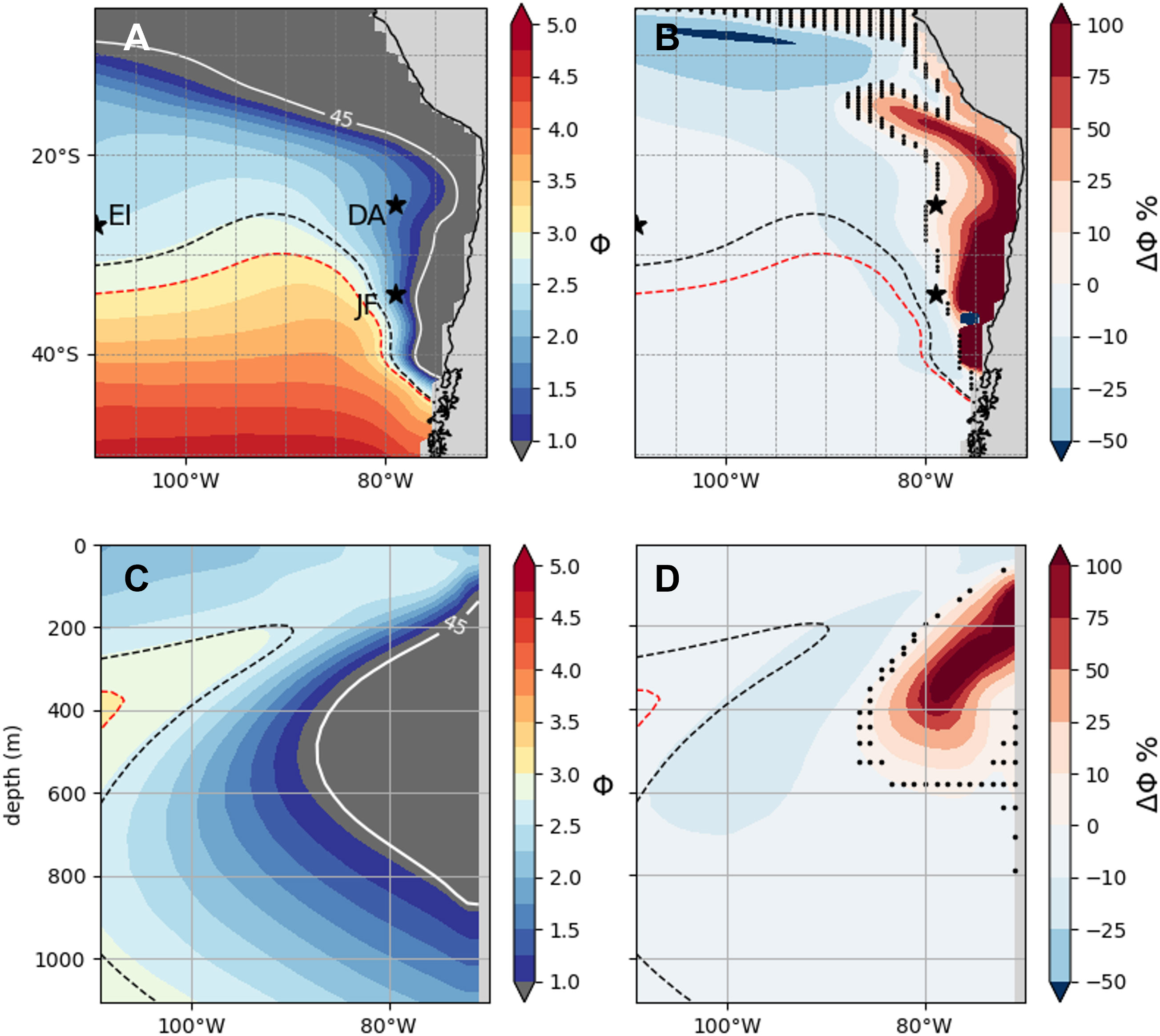
Figure 2 Metabolic index of the model species (Ф_model). Mean metabolic Index (A, C) and change (ΔΦ) between the present and future climate (B, D) at 200m (A, B) and 26°S (C, D).The dashed isocontours indicate the position of the mean Φ_crit (=3) in the present (black) and the future (red) climates. The white line is the mean 45 mmol.m^-3 oxygen isocontour of the future climate. The dark grey shading is where Φ< 1. The dark stars represent Juan Fernandez (JFA), the Desventuradas Archipelagos (DA) and Easter Island (EI). The black dots (B, D) indicate where ΔΦ is not significant across the 34 members (Wilcoxon rank sum test p < 0.05).

Further sensitivity tests show a high dependency of the magnitude of Φ to the trait A₀ due to the linear relationship between Φ and A₀ (Figures S7A, C) but a weaker sensitivity to E₀ (Figures S7B, D). This can be illustrated with the shrimp O. spinosus (Figure S8) which shows higher values of Φ with a ratio Φ_model/Φ_shrimp ≈ A_0,model/A_0,shrimp. This also demonstrates that the position of the mean Φ_crit strongly varies within the documented range of traits (Figure S9). Therefore, given the lack of observed values in (A₀, E₀), mean Φ_crit (=3) cannot be used here with confidence to project mean changes in viable metabolic habitat in the SEP. We show hereafter that CV_Φ has much less dependence to A₀ and E₀, which makes it more convenient for addressing this issue given the scarcity of data in the SEP.

3.2. Climate velocities of the metabolic index (CV_Ф)

3.2.1. Pattern of CV_Ф

We estimate here the speed and direction of the future displacement of the metabolic habitat described by Φ (see section 2.3) for the model species (Figure 3). The pattern of the spatial gradient of Φ_model indicates that it is constrained by pO₂ (see eq.4). More specifically, it has bimodal spatial distribution constrained by the OMZ (Figure 3B, 45 mmol.m^-3 blue isoline) and by oxygenated waters (Figure 3B, 150 mml.m^-3 blue isoline). On the one hand, the OMZ is characterized by a high horizontal gradient area where Φ changes are in the higher range of 0.5 Φ/100km (in the outer edges of the OMZ) to 1.5 Φ/100km (between 30°S and 40°S) for the model species. This area characterizes a metabolic barrier as Φ varies abruptly there, separating two very distinct environments, i.e. separating hypoxic species (Vaquer-Sunyer and Duarte, 2008) and normoxic species. Juan Fernandez Archipelago (JFA) and the Desventuradas Islands Archipelago (DA) are within the area of high gradient with respectively 0.5 and 1.5 Φ/100km. On the other hand, oxygenated waters are characterized by a very weak gradient in the range of 0 to 0.5 Φ/100km with a mean spatial gradient there of ~0.1 Φ/100km indicating that the metabolic environment is stable and similar over long distances.

FIGURE 3

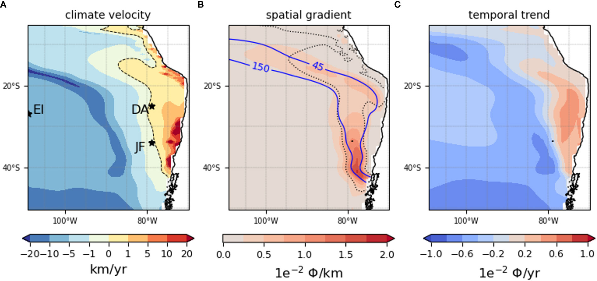
Figure 3 Climate velocities, spatial gradient and temporal trend of the Metabolic Index Φ of the model species at 200m over 2006-2100. For climate velocities (A), the dashed line is where CV_Φmodel = 0 km.yr^-1. For the spatial gradient (B), the dotted line delimits the region for which |CV|< 1 km.yr^-1. The blue isolines represent the 45 (OMZ) and 150 (oxygenated waters) oxygen isocontours in mmol.m^-3. (C) are the temporal trend. The dark stars represent Juan Fernandez (JFA), the Desventuradas Archipelagos (DA) and Easter Island (EI).

The trends (Figure 3C) are positive on the eastern side of the basin and negative in the open ocean, covering the majority of the SEP, consistent with that of the oxygen trends at this depth (Figure 1). Positive trends represent locally an increase of up to 0.8 units (Figure 3C) by 2100 where Φ is lowest (Φ<2, Figures 2A, C). West of 80°W negative trends represent a decrease of up to 0.1 units and up to 0.5 Φ by 2100. Trends in the key ecoregions of JFA and DA are weak.

CV_Φ,model are positive east of the basin consistent with temporal trends. They are mostly weak (i.e. |CV_Φ|<1 km.yr^-1, Figure 3B dotted line envelope) within the OMZ. There, the displacement of habitat represented by CV_Φ,model is controlled by the spatial distribution of Φ_model (spatial gradient). In areas of slow positive/negative velocities, analogue metabolic environments are found “close” (within 100km) and in the direction of an increasing/decreasing gradient (Figure S10). This translates into a short displacement of species to find metabolic conditions analogous to those of their occupied habitat. CV_Φ,model is locally high (>10 km.yr^-1) and positive in the coastal region of Chile between 30°S and 40°S and off Peru at 20°S as the result of the combination of high temporal trends and a weak spatial gradient. There, marine species will benefit from a fast temporal Φ increase (high trend) in a stable environment (weak spatial gradient). Oxygenated waters are characterized by relatively high negative velocities (5km.yr^-1) due to temporal trends in the higher range and weak gradients. Faster negative velocities (< -10 km.yr^-1) are observed in the southernmost part of the basin and adjacent to the OMZ where the most negative trends are found.

3.2.2. Drivers of CV_Φ

We now evaluate the relative contributions of temperature and oxygen trends to CV_Φ (see section 2.3.2) in order to characterize the drivers behind the projected habitat dynamic and given current uncertainties in oxygen trend in particular to gain confidence in the assessment of areas of climate exposure (section 4.1).

Figure 4 represents the relative contribution of pO₂ and temperature to CV_Φ. A negative sign implies a CV_Φ decrease and conversely (in %, see section 2.3.2 and Supplementary Text). There are very contrasting behaviors between the OMZ and oxygenated waters and between the subsurface and deeper waters. At 200m (Figures 4A, B), positive oxygen trends are the main driver of CV_Φ in the OMZ with an incursion into equatorial waters (>75%). Negative oxygen trends contribute at least to 50% of the change in CV_Φ in the northernmost part of the SEP (south of 20°S) and along the OMZ border. On the contrary, temperature trends are the main driver in the south-end of the SEP with a contribution superior to 75%. At 26°S (Figures 4C, D), in the OMZ core, the trends in oxygen is the main driver (> 75%) and contributes to an increase in CV_Φ. In oxygenated waters however ([0₂] > 150 mmol.m^-3), oxygen trends contribute more (>50%) than temperature trends below 400m whereas temperature trends are the main driver in the thermocline (> 75% above ~400m).

FIGURE 4

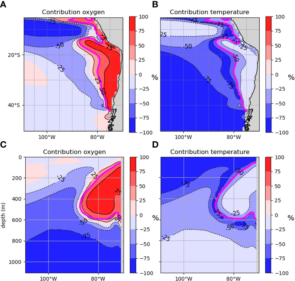
Figure 4 Contributions (in %) of the trends in oxygen and temperature to CV_Ф of the model species. At 200m (A, B) and 26°S (C, D). The Eq. 6 of section 2.3.2 is used for this calculation. A negative/positive sign means a negative/positive contribution of the driver. A driver is considered a main driver when % > 75, and O₂ and temperature contribute equally when % = 50. The magenta contour is where [CV]= 0. km.yr^-1 signaling the transition area between positive and negative velocities.

There is an approximately equal contribution of both drivers to CV_Φ around the transition zone between positive and negative oxygen trends (magenta contour Figure 4). CV_Φ undergo either the additive negative effects of warming and deoxygenation, or, the compensatory effect of positive trends in oxygen and warming. Note that the effect of warming here will be modulated by E₀ greatly affecting the sign and magnitude of the velocities.

3.3. Sensitivity analysis

In this section we analyze how CV_Φ varies as a function of E₀ and natural variability. This allows us to assess the confidence level one can have in CV_Φ,model to infer future displacement of local metabolic environment. We show in particular that CV_Φ,model is statistically comparable to CV(E₀)_mean and an ensemble of real species. We also identify regions where natural variability is likely to contribute to the uncertainties in the estimate in CV_Φ and habitat changes. This will serve as material for guiding our method to quantify changes in habitat and for discussing our results (section 4.1).

3.3.1. Representativity of the model species

In this section, we explore the sensitivity of CV_Φ to the physiological trait E₀ in order to infer if our results can be generalized to the case of real species. We first analyze the uncertainty associated to CV_Φ across the E₀ range (Figure 5). Error_CV(E₀) (Figures 5A, C, see method section 2.4.1) indicates the weakest sensitivity of CV(E₀) (s.d. < 1 km.yr^-1) in the OMZ domain (white contours, Figures 5A, C) and a relatively stronger sensitivity (s.d. > 1 km.yr^-1) in the thermocline (Figure 5C) beyond the OMZ limits ([O₂] > 150 mmol.m^-3, Figures 5A, C). Furthermore, CV_Φ,model, CV(E₀)_Eo>0 and CV(E₀)_mean show statistically comparable bimodal distributions (Figure 6). CV_Φ,model distribution slightly shifts to more negative velocities for CV_Φ,model compared to CV(E₀)_mean. This can be verified with the velocities of the shrimp O. spinosus (Figure S11) whose velocities mirror that of CV_Φ,model despite a weaker E₀ (E_0,shrimp = 0.19 eV vs. E_0model = 0.4 eV). CV(E₀) with negative E₀ (light grey lines, Figure 6) are however not comparable as negative E₀ tend to increase Φ under warming trends (see also Figure S12 and section 3.2.2) compensating deoxygenation. Lastly, the ratio CV(E₀)_mean/CV_Φ,model is weak (<10%) in all the SEP except in the transition area (Figures 5B, D).

FIGURE 5

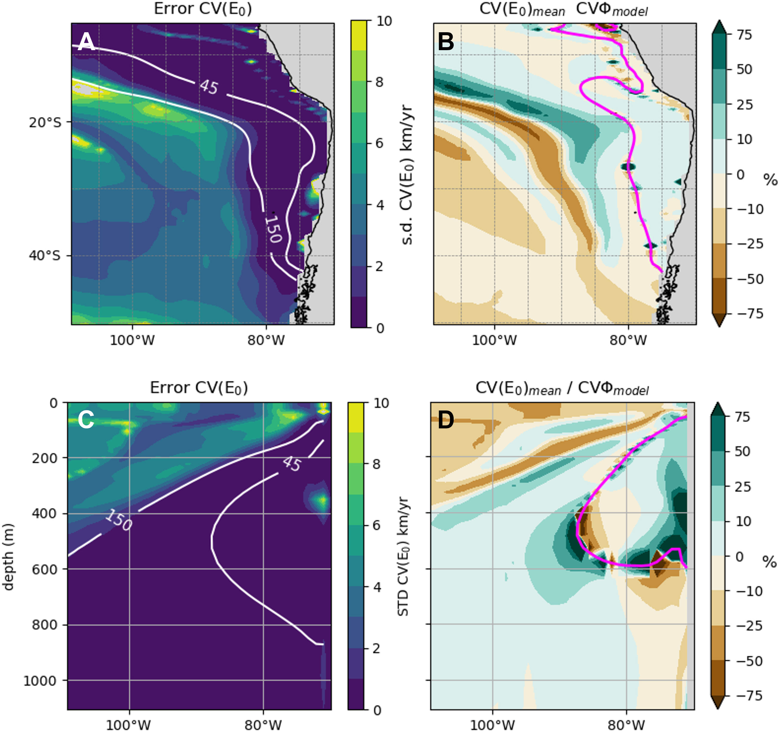
Figure 5 Sensitivity of CV_Φ to the physiological trait E₀. At 200m (top) and 26°S (bottom). (A, C) provide the absolute uncertainty and (B, D) the relative uncertainty (see method section 2.4.1). The range of E₀ used is provided in Figure S4. (B, D) represent the relative difference between CV(E₀)_mean and CV_Φ,model in %. The white contours indicate the 45 and 150 oxygen isocontours (mmol.m^-3). The magenta lines indicate where CV_Ф,model = 0 km.yr^-1 (i.e. the transition area).

FIGURE 6

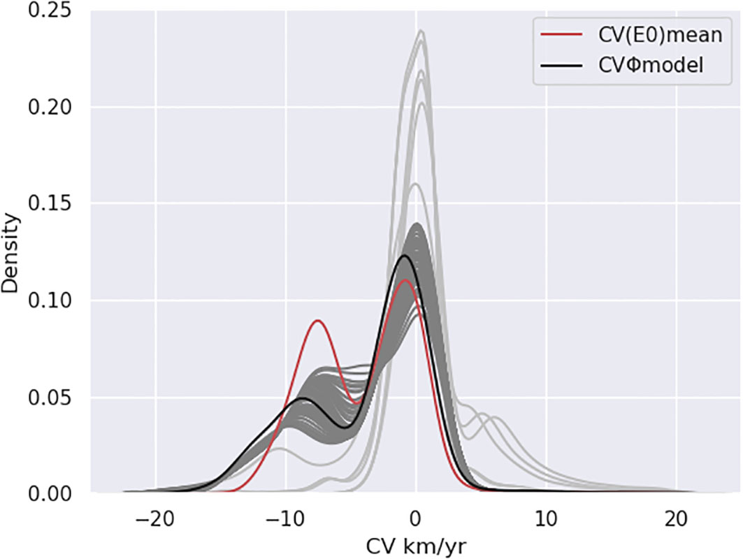
Figure 6 Pdf of climate velocities of the metabolic index at 200m. For CV_Φmodel (black) and CV(E₀)_mean (red). For the 71 species in grey with positive E₀ (dark grey) and negative E₀ (light grey).

In fact, the highest uncertainty occurs where the contribution of oxygen and temperature to CV_Φ are equal (i.e. OMZ border and transition between positive and negative velocities, see magenta contour Figure 4). There, E₀ affects the near balance between the contributions of oxygen and temperature to CV_Φ so that any changes caused by E₀ affect significantly the sign and magnitude of CV_Φ, especially in this low velocity area. For example, increasing E₀ strengthens the effect of warming over that of positive oxygen trends so that CV_Φ tend to become positive, and conversely. Varying values of E₀ cause ultimately a shift in the median of CV_Φ (Figure S12) and hence displace the frontiers between positive and negative velocities. This effect is also visible when comparing CV(E₀)_mean to CV_Φ,model where the relative difference in magnitude is >25% (Figures 5B, D). Hence, estimating the speed of habitat displacement with CV_Φ is more trait sensitive in the transition area where the change in sign of velocities occurs. Hence, we argue that CV_Φ,model is quite representative of the mean displacement of an ensemble of real species, except in the transition area highly sensitive to E₀ because of the way it affects the equal contribution of oxygen and temperature trends to changes in Φ. This is particularly valuable and useful as very few species ecophysiotypes are documented.

3.3.2. Uncertainty in CV_Φ due to natural variability

The CESM-LE offers the opportunity to estimate uncertainties associated to natural variability that accounts for variations in the long-term mean associated with natural modes of variability in the SEP such as ENSO or the Interdecadal Pacific Oscillation (Henley et al., 2015). This type of uncertainty can be derived from the estimate of the standard deviation of CV_Φ amongst the 34 realizations (i.e. members) of the same model.

We estimated the absolute (Figures 7A–C and Figures S13A–C) and relative (Figures 7D–F; Figures S13D–F) uncertainty associated to natural variability, and whether it originates from the oxygen or temperature fields (see method in section 2.4.2) in order to provide guidance for determining areas of climate change exposure (see section 4.1). The results indicate a vast share of the domain where natural variability can induce fluctuations in the long-term mean of temperature and oxygen and thus CV_Φ (Figures 7A–C; Figures S13A–C). Error_CV_Φ_all appears to be mostly related to Error_CV_Φ_O₂ within the OMZ and slightly beyond the OMZ limit. Over the rest of the domain, Error_CV_Φ_T is comparatively strong in oxygenated waters above 200m (Figure 7C; Figure S13C). Where interannual variations in oxygen and temperature are large, such as along the coast of South America where there is an efficient ENSO oceanic teleconnection (Sprintall et al., 2020) and over the subtropical pressure system where tropical and extra-tropical atmospheric teleconnections modulate the oceanic circulation, large uncertainties are expected. However since CV_Φ tend to have large values (in absolute value) there, the relative uncertainty remains weak (Figures 7D–F; Figures S13D–F). The regions of large relative uncertainty are in fact found where CV_Φ is relatively weak (i.e. |CV|< 1 km.yr^-1, see dotted contours Figure 3B), which corresponds to a zone approximately bordering the OMZ limits in its interior to the South of 20°S and expanding to the Peru upwelling system and equatorial region to the North. We define this area as the “transition area” (magenta contour Figures 7D; S13D) where uncertainty due to natural variability limits our confidence in the estimate of CV_Φ. That said, confidence in estimate of CV_Φ remains strong in oxygenated waters and the OMZ and can be relied on to infer future habitat change.

FIGURE 7

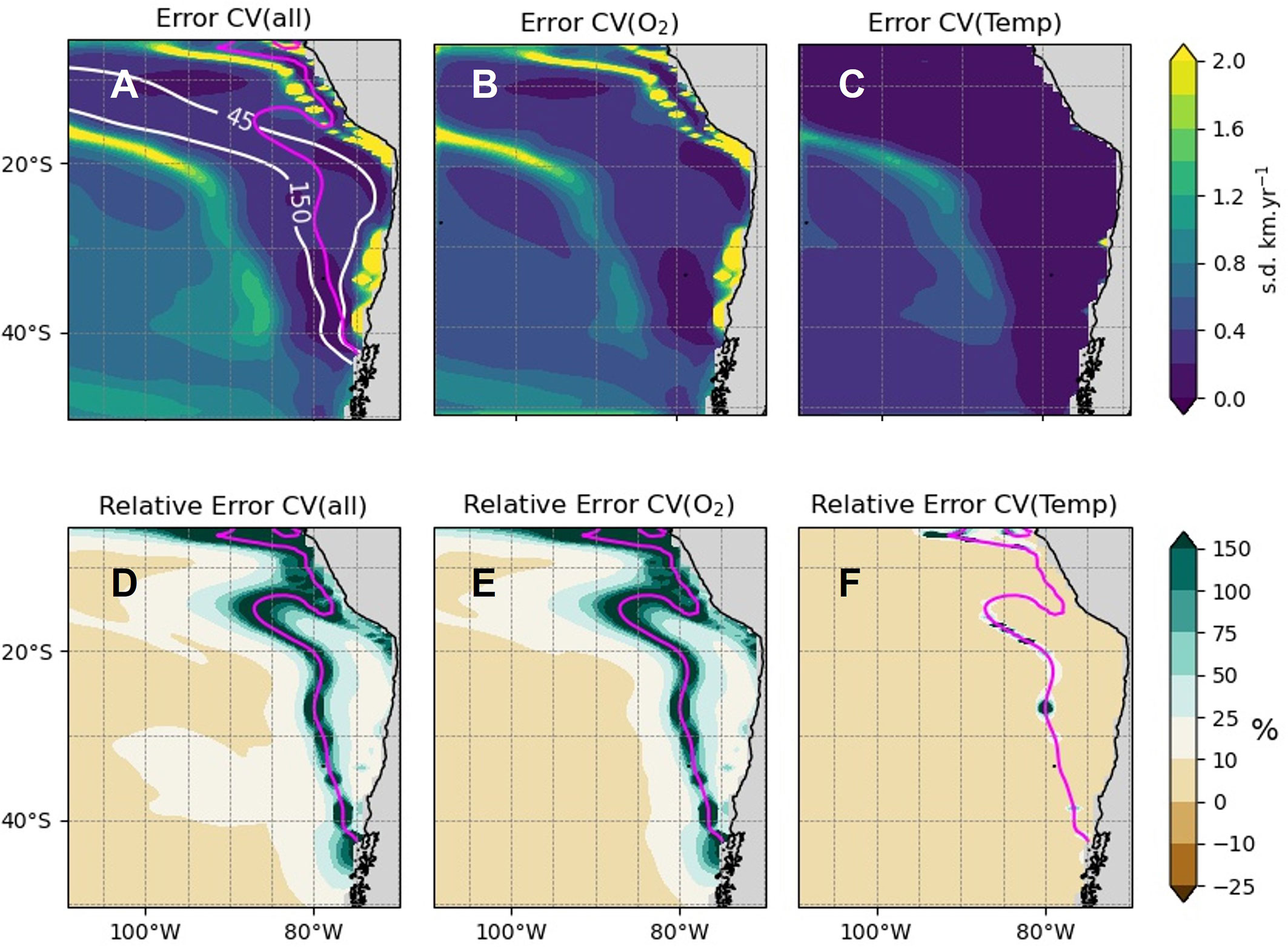
Figure 7 Uncertainty of CV_Φ associated to natural variability at 200m. Error_CV_Φ_all, Error_CV_Φ_O₂ and Error_CV_Φ_T correspond to the uncertainty associated to natural variability and the oxygen-trend and temperature-trend induced uncertainty, respectively. (A–C) provide the absolute error and (D–F) the relative error (%, see method section 2.4.2). The white contours are where [O₂] = 45 and 150 mmol.m^-3. The magenta dashed contours indicate the transition area (|CV_Φmodel|= 0 km.yr^-1).

4. Discussion

While our results illustrate the potential in using CV_Φ for inferring changes in habitat, the characteristics of the SEP region (i.e. low consensus in deoxygenating trend in the OMZ region amongst climate models, and scarcity of physiological data) limit a quantitative inference of future habitat. Still, we argue that CV_Φ can be useful for inferring broad regions where metabolic conditions change and therefore of potential metabolic refugia.

4.1. Inferring change in habitat from CV_Φ: Areas of climate change exposure

Taking advantage of the model species representativity, we now combine the information given by the velocities, spatial gradient and temporal trends to illustrate how CV_Φ can help define broad areas of exposure to climate change. Our approach is based on the choice of threshold values for each of these three quantities. This choice is here somewhat subjective since we work with a model species, but it could be adjusted in case studies.

We define areas of exposure to climate change based on the sign and magnitude of the velocities (Figure 8). Positive trends indicate a favorable evolution of the local metabolic environment (maintained to increased aerobic scope). However, negative trends indicate a reduction of aerobic scope and therefore an increased probability for Φ to fall below Φ_crit. Hence local trends indicate the level of pressure species face at any location. The magnitude of the velocity is used based on an arbitrary threshold equal to 1 km.yr^-1 (Figure 8). This threshold value is convenient because it allows visualizing where the spatial gradient in Φ is larger or smaller than its long-term trend, i.e. where the local rate of change is larger than the spatial distribution of Φ. Therefore, slow velocities indicate that local changes can be “compensated” by close analog environments, whereas fast velocities indicate that local analogues will be found >100 km by 2100. Hence, we define four areas of incremental risk (Figure 8). Area I is the safest with fast positive velocities and therefore a fast increase in metabolic index locally. Area II is moderately safe; the metabolic environment improves at a slow rate and local analogue environments are found “close”. Area III is moderately at risk with a decrease of Φ but with close analogue environments. Finally, Area IV is most at risk with the fastest negative velocities. Locally, the metabolic environment degrades at a fast rate suggesting a short emergence time for negative conditions (e.g. Φ_crit). Lastly, we define an area of high uncertainty which includes the uncertainty associated to traits (Figures 5B, D) and associated to natural variability (Figures 7D, S13D) and where the relative error exceeds 25%. This area encompasses the changes in the contribution of drivers to CV_Φmodel, and allows to capture the coupled effect of temperature and E₀ (Figure 5) and the change in sign of oxygen trends (Figure 7).

FIGURE 8

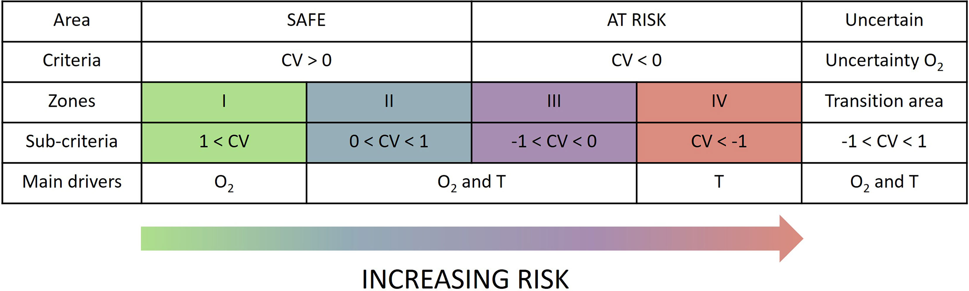
Figure 8 Definition of areas of climate change exposure. Areas with positive or negative velocities are classified as “safe or “at risk”. We also distinguish area of slow velocities driven by the spatial gradient (|CV|< 1km.yr^-1, zones II and III) and areas of fast velocities driven by the temporal gradient (|CV| > 1 km.yr^-1, zones I and IV). The transition area defined by a high uncertainty related to natural variability and physiological traits is classified as uncertain. To each of these areas correspond main drivers (i.e. oxygen (O₂) and temperature (T) as analyzed in section 3.2.2.

Based on these definitions, we illustrate the potential consequences for marine species and habitat in the OMZ and its border, the open ocean and seamounts (Figure 9A) and along a vertical section at 26°S (Figure 9B, see also Figure S14 for a vertical section of the horizontal velocities at 26°S) which allows to visualize potential risks for the 2D horizontal marine metabolic habitats at depth.

FIGURE 9

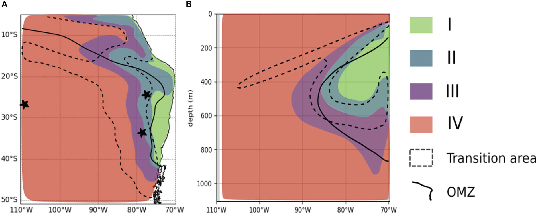
Figure 9 Areas of climate change exposure. Areas of climate exposure in the SEP at 200m (A) and the vertical representation at 26°S (B) derived from the horizontal velocities. We defined areas of climate exposure based on the components of the climate velocities of Ф using the model species. Areas I and II designate “safe” areas based on positive trends in Ф. Areas III and IV designate “at risk” areas based on negative trends in Ф. Areas II and III are areas of slow velocities (|CV|< 1 km.yr^-1) where the spatial gradient controls the magnitude of CV_Φ over the temporal trends. The transition area (dashed envelope) is the area most subjected to uncertainty in the sign and magnitude of the velocity due to high uncertainty in the sign of oxygen trends and the effect of E₀. The black and solid contour represents the OMZ limit at 45 mmol.m^-3. Note that the OMZ contour also coincides with Φ = 1.

Areas I and II spread along coastal waters and over the OMZ domain at 200m and in the OMZ core (Figures 9A, B). Consequently, species living and accumulating at the lower OMZ borders (Paulmier et al., 2021) or demersal or benthic (Levin and Gallo, 2019), may find less stressful and a more stable environment which should preserve species abundance. Area II spreads across the OMZ border and represents a horizontal compression of the OMZ (defined by the 45 mmol.m^-3 isocontour) between 20°S and 40°S at 200m. There, hypoxia tolerant species inhabiting the outer edges of the OMZ (Birk et al., 2019; Roman et al., 2019) may extend their habitat distribution. Area I and II are further characterized by very low Φ (Φ<2, Figure 2B) and by species adapted to hypoxic environment. Therefore, it is unlikely that hypoxia intolerant species migrate to area II. Since changes are mainly driven by oxygen (Figures 4A, C), species sensitive to temperature are more likely to sustain the weak changes in Φ attributed to increasing temperature. Hence, species composition and richness should be preserved.

Area III is characterized by slow negative velocity and is located along the OMZ border. In area III, the temporal trends are in the lower range, meaning a slower decrease of Φ and therefore a limited compression of their habitat. Besides, being in a high gradient area, species would find analogue conditions a few kilometers away in the direction of the open ocean with more oxygenated waters. However, this needs to be taken with caution, as what matters for a species is the distance between Φ and its respective Φ_crit. Indeed, slow negative velocities could still be fast enough to cause deleterious changes as many species live close to their physiological limits (Tremblay et al., 2020; Wishner et al., 2020) and would therefore be weakly tolerant to environmental changes. Species at different ontogenetic stages are not responding equally against environmental changes. Organisms at embryonic, larval and spawning stages are less tolerant to elevated temperatures (Dahlke et al., 2020) and low oxygen conditions (Breitburg, 2002) than adults in marine environments. This is especially important as changes in area III are driven by both temperature increase and oxygen loss. Area IV covers the west of the SEP (Figure 9A) and most of the vertical range at depth (Figure 9B), from shallow waters above the OMZ to all the water column to the west. In area IV, changes are also driven by both drivers. Area IV is all the more at risk as analogue environments will be found over long distances (>100km away by 2100), suggesting long southward migrations (Figure S10). However, area IV is also characterized by the highest Φ, so that habitats may remain viable as long as Φ remains above Φ_crit. Equatorial waters and coastal Peruvian waters are located in areas III and IV which may drive fisheries species away to the south and from the coasts. According to our results, artisanal and industrial fisheries as well as aquacultures from coastal waters off Peru and Chile, mostly located in areas III and IV, are at risk.

Lastly, the transition area (Figure 9, dashed envelope) encompasses seamounts areas such as DA and JFA and Exclusive Economic Zones where fishing exploitations occur. These seamounts (Yanez et al., 2009) are known to act as stepping stones for species dispersion (i.e., Salas y Gomez Ridge), by diverse and highly vulnerable ecosystems and by the highest number of endemic species (Yanez et al., 2009; Dyer and Westneat, 2010; Friedlander et al., 2016; Mecho et al., 2021). Islanders’ local economy is based on the artisanal fisheries (Friedlander and Gaymer, 2021), such as the Juan Fernandez lobster. Environmental changes could be harmful to these communities if marine species were to migrate or perish. Besides, fishing grounds could be displaced beyond reasonable distances out of reach for these communities which use small boats and are not capable to sail long distances. Additionally, these islands are characterized by a high level of connectivity at larval stage. Changes there could reduce the migratory fluxes at the larval stage (Porobic et al., 2012; Porobic et al., 2013) of several species such as the sea urchin Centrostephanus sylviae (Veliz et al., 2021) or the Juan Fernandez lobster Jasus frontalis (Ernst et al., 2013), a fishery target species. Making use of species traits in these areas would reduce the uncertainty in the sign of the changes in these areas.

4.2. Cautionary consideration for the use of the metabolic index

While the metabolic index can be used as an indicator of exposure to climate change, it is important to discuss its relevance for the OMZ waters and for some species. When environmental pO₂ is limiting the maximum metabolic rate (MMR), Φ is equivalent to the measure of the factorial aerobic scope (FAS; (Seibel and Deutsch, 2020; Seibel and Birk, 2022) which is the factorial difference between maximum metabolic rate (MMR) and standard metabolic rate (SMR). The majority of species that have been studied in the literature have evolved in shallow, coastal waters where pO₂ is routinely near air-saturation, regardless of temperature. The oxygen supply capacity for each of those species has evolved to meet maximum demand at the prevailing pO₂, which for most of them is near air-saturation. As a result, the critical oxygen pressure for maximum metabolic rate (P_cmax) is also near air-saturation and both, MMR and FAS, decline in proportion to pO₂ below P_cmax, again regardless of temperature (Seibel and Deutsch, 2020). For such species, the metabolic index (simplified as pO₂/P_crit at any given temperature), is a valuable estimate of the aerobic scope for activity. For vertical migrators, and likely other mesopelagic species in the upper water column, pO₂, temperature and light are strongly correlated along a depth gradient. Metabolic demand for activity decreases with light and depth (Childress, 1995), such that MMR and FAS are highest in warm water and decline strongly with depth and temperature. P_cmax is also highly sensitive to temperature and tends to decline with depth at a similar rate as pO₂ below the thermocline (Seibel and Birk, 2022). At the lower oxycline, oxygen begins to increase while temperature continues to decline with depth. For species living there, E₀ is strongly negative and hypoxia tolerance is improved in warm water (Wishner et al., 2018). P_cmax is not readily predictable for those species. Therefore P_cmax may be higher or lower than ambient pO₂ at depth, but it will always be much less than air-saturation in oxygen minimum zone species. When P_cmax < pO₂, the metabolic index overestimates aerobic scope, which is, instead, dependent only on temperature. Species can migrate to keep within the boundary conditions defining the ecological niches or can persist locally in new or changing habitats through both phenotypic plasticity and adaptive evolution (Anderson et al., 2012; Munday, 2014) as a response to rapidly changing environmental conditions (Baltar et al., 2019). Metabolic traits of SEP mesopelagic species have changed as a response to a unique environment and thus may not be captured by a mean ecophysiotype model representative of a broad range of species. Thus, P_cmax must be known for each non-coastal or shallow species before the metabolic index can be applied with confidence.

4.3. Concluding remarks

We showed here that CV_Φ conveys useful information to define potential marine habitat changes and distribution shifts, providing an overview on how broad environmental niches would evolve in space and time under climate change for a broad range of species inhabiting the SEP (see Figure 9). We also manage to identify regions where the confidence level in the estimate of CV_Φ is likely to be the largest considering current regional uncertainties in deoxygenation trends in the SEP as simulated by current-generation climate models and considering the sensitivity of CV_Φ to the physiological traits E₀. Using species specific ecophysiotypes can additionally support CV_Φ for guiding management approaches to conservation (Brito-Morales et al., 2018). Indeed, defining the distance between the local Φ (at one location) and the limit of viable habitat (Φ_crit) would enable: 1) emergence time estimations of negative conditions (Φ<Φ_crit) and therefore time available for adaptation and action in critical locations (for both marine species and human systems) and 2) velocities and trajectories of critical habitat which inform on the displacement of boundaries of the metabolic viable habitat which varies from one species to another. Using CV_Φ with species specific ecophysiotypes would also help reduce the uncertainty of CV_Φ in key areas of the SEP. Other additions to the tools for designing MPA include information coming from vertical climate velocities. Indeed, vertical velocities for species performing vertical migrations or species occupying a range of depths would provide useful information regarding the likelihood of vertical migrations especially when vertical habitat seems at risk as suggested by our preliminary results. It was shown that vertical velocities have a lower order of magnitude (m.dec^-1, Jorda et al., 2020) and therefore, are not directly comparable to horizontal velocities, placing them beyond the scope of this paper. Lastly, recent findings (Seibel and Birk, 2022) suggest that additional physiological information (P_cmax) may be necessary to determine whether the metabolic index can accurately be applied to vertical migrators and oceanic species (see section 4.2). In addition to the metabolic index, other indicators such as the Aerobic Growth Index (AGI, Clarke et al., 2021b) or simply the FAS (Seibel and Birk, 2022) may be valuable alternatives to consider. These represent directions for future investigations.

Data availability statement

Publicly available datasets were analyzed in this study. Thisdata can be found here: https://github.com/aparouffe/SEP_habitability. The datasets used in this study are available at: https://www.cesm.ucar.edu/projects/community-projects/DPLE/datasets.html The scripts for the climate velocity computations areavailable in a GitHub repository: https://github.com/aparouffe/SEP_habitability.

Author contributions

VG and BD initiated the study. APar performed the computations and wrote the manuscript. All authors discussed and interpreted the results and provided input to the manuscript. All authors contributed to the article and approved the submitted version.

Funding

VG, BD, and IM acknowledge support from the United States National Science Foundation grant OCE-1840868 to the Scientific Committee on Oceanic Research (SCOR, United States). They are supported by the SCOR WG 155 on EBUS and they acknowledge support from ANID (Concurso de Fortalecimiento al Desarrollo Científico de Centros Regionales 2020-R20F0008-CEAZA). BD acknowledges support from ANID (Eclipse ACT210071 and COPAS COASTAL FB210021). VG and BD are supported by the CE2COAST project funded by ANR (FR), BELSPO (BE), FCT (PT), IZM (LV), MI (IE), MIUR (IT), Rannis (IS) and RCN (NO) through the 2019 “Joint Transnational Call on Next Generation Climate Science in Europe for Oceans” initiated by JPI Climate and JPI Oceans. APar, VG, and BD are also supported by the EU H2020 FutureMares project (Theme LC-CLA-06-2019, Grant agreement No 869300). BD, CP, and DV acknowledge also support from ANID (Grants 1190276 and 1191606).

Acknowledgments

We would like to thank Dr. K. von Schuckmann for early discussion on the results. We warmly thank Pr. Brad Seibel for sharing his knowledge and most recent findings into the application of the metabolic index to vertical migrators and providing constructive feedback on our manuscript.

Conflict of interest

The authors declare that the research was conducted in the absence of any commercial or financial relationships that could be construed as a potential conflict of interest.

Publisher’s note

All claims expressed in this article are solely those of the authors and do not necessarily represent those of their affiliated organizations, or those of the publisher, the editors and the reviewers. Any product that may be evaluated in this article, or claim that may be made by its manufacturer, is not guaranteed or endorsed by the publisher.

Supplementary material

The Supplementary Material for this article can be found online at: https://www.frontiersin.org/articles/10.3389/fmars.2022.1055875/full#supplementary-material

References

Anderson J. T., Inouye D. W., McKinney A. M., Colautti R. I., Mitchell-Olds T. (2012). Phenotypic plasticity and adaptive evolution contribute to advancing flowering phenology in response to climate change. Proc. R. Soc B. 279, 3843–3852. doi: 10.1098/rspb.2012.1051

CrossRef Full Text | Google Scholar

Arana P., Ziller S. (1985). “Antecedentes generales sobre la actividad pesquera realizada en el archipiélago de Juan fernández,” in Investigaciones marinas en el archipiélago de Juan fernánde (Escuela de Ciencias del Mar Universidad Catolica de Valparaiso), 125–152.

Google Scholar

Baltar F., Bayer B., Bednarsek N., Deppeler S., Escribano R., Gonzalez C. E., et al. (2019). Towards integrating evolution, metabolism, and climate change studies of marine ecosystems. Trends Ecol. Evol. 34, 1022–1033. doi: 10.1016/j.tree.2019.07.003

PubMed Abstract | CrossRef Full Text | Google Scholar

Bertrand A., Chaigneau A., Peraltilla S., Ledesma J., Graco M., Monetti F., et al. (2011). Oxygen: A fundamental property regulating pelagic ecosystem structure in the coastal southeastern tropical pacific. PloS One 6, e29558. doi: 10.1371/journal.pone.0029558

PubMed Abstract | CrossRef Full Text | Google Scholar

Birk M. A., Mislan K. A. S., Wishner K. F., Seibel B. A. (2019). Metabolic adaptations of the pelagic octopod japetella diaphana to oxygen minimum zones. Deep Sea Res. Part I: Oceanographic Res. Papers 148, 123–131. doi: 10.1016/j.dsr.2019.04.017

CrossRef Full Text | Google Scholar

Bopp L., Resplandy L., Orr J. C., Doney S. C., Dunne J. P., Gehlen M., et al. (2013). Multiple stressors of ocean ecosystems in the 21st century: projections with CMIP5 models. Biogeosciences 10, 6225–6245. doi: 10.5194/bg-10-6225-2013

CrossRef Full Text | Google Scholar

Breitburg D. (2002). Effects of hypoxia, and the balance between hypoxia and enrichment, on coastal fishes and fisheries. Estuaries 25, 767–781. doi: 10.1007/BF02804904

CrossRef Full Text | Google Scholar

Brito-Morales I., García Molinos J., Schoeman D. S., Burrows M. T., Poloczanska E. S., Brown C. J., et al. (2018). Climate velocity can inform conservation in a warming world. Trends Ecol. Evol. 33, 441–457. doi: 10.1016/j.tree.2018.03.009

PubMed Abstract | CrossRef Full Text | Google Scholar

Brito-Morales I., Schoeman D. S., Molinos J. G., Burrows M. T., Klein C. J., Arafeh-Dalmau N., et al. (2020). Climate velocity reveals increasing exposure of deep-ocean biodiversity to future warming. Nat. Climate Change 10, 576–581. doi: 10.1038/s41558-020-0773-5

CrossRef Full Text | Google Scholar

Burrows M. T., Schoeman D. S., Richardson A. J., Molinos J. G., Hoffmann A., Buckley L. B., et al. (2014). Geographical limits to species-range shifts are suggested by climate velocity. Nature 507, 492–495. doi: 10.1038/nature12976

PubMed Abstract | CrossRef Full Text | Google Scholar

Cabré A., Marinov I., Bernardello R., Bianchi D. (2015). Oxygen minimum zones in the tropical pacific across CMIP5 models: mean state differences and climate change trends. Biogeosciences 12, 5429–5454. doi: 10.5194/bg-12-5429-2015

CrossRef Full Text | Google Scholar

Cai W., Santoso A., Collins M., Dewitte B., Karamperidou C., Kug J.-S., et al. (2021). Changing El niño–southern oscillation in a warming climate. Nat. Rev. Earth Environ. 2, 628–644. doi: 10.1038/s43017-021-00199-z

CrossRef Full Text | Google Scholar

Carréric A., Dewitte B., Cai W., Capotondi A., Takahashi K., Yeh S.-W., et al. (2020). Change in strong Eastern pacific El niño events dynamics in the warming climate. Climate Dynamics 54, 901–918. doi: 10.1007/s00382-019-05036-0

CrossRef Full Text | Google Scholar

Carstensen D., Riascos J. M., Heilmayer O., Arntz W. E., Laudien J. (2010). Recurrent, thermally-induced shifts in species distribution range in the Humboldt current upwelling system. Mar. Environ. Res. 70, 293–299. doi: 10.1016/j.marenvres.2010.06.001

PubMed Abstract | CrossRef Full Text | Google Scholar

Cheung W. W. L., Lam V. W. Y., Sarmiento J. L., Kearney K., Watson R., Pauly D. (2009). Projecting global marine biodiversity impacts under climate change scenarios. Fish and Fisheries 17, 235–251. doi: 10.1111/j.1467-2979.2008.00315.x

CrossRef Full Text | Google Scholar

Childress J. J. (1995). Are there physiological and biochemical adaptations of metabolism in deep-sea animals? Trends Ecol. Evol. 10, 30–36. doi: 10.1016/S0169-5347(00)88957-0

PubMed Abstract | CrossRef Full Text | Google Scholar

Clarke T. M., Reygondeau G., Wabnitz C., Robertson R., Ixquiac-Cabrera M., López M., et al. (2021a). Climate change impacts on living marine resources in the Eastern tropical pacific. Divers. Distrib 27, 65–81. doi: 10.1111/ddi.13181

CrossRef Full Text | Google Scholar

Clarke T. M., Wabnitz C. C. C., Striegel S., Frölicher T. L., Reygondeau G. (2021b). Aerobic growth index (AGI): An index to understand the impacts of ocean warming and deoxygenation on global marine fisheries resources. Prog. Oceanogr 195, 102588. doi: 10.1016/j.pocean.2021.102588

CrossRef Full Text | Google Scholar

Clark M. R., Rowden A. A., Schlacher T., Williams A., Consalvey M., Stocks K. I., et al. (2010). The ecology of seamounts: Structure, function, and human impacts. Annu. Rev. Mar. Sci. 2, 253–278. doi: 10.1146/annurev-marine-120308-081109

CrossRef Full Text | Google Scholar

Cowles D. L., Childress J. J., Wells M. E. (1991). Metabolic rates of midwater crustaceans as a function of depth of occurrence off the Hawaiian islands: Food availability as a selective factor? Mar. Biol. 110, 75–83. doi: 10.1007/BF01313094

CrossRef Full Text | Google Scholar

Dahlke F. T., Wohlrab S., Butzin M., Pörtner H.-O. (2020). Thermal bottlenecks in the life cycle define climate vulnerability of fish. Science 369, 65–70. doi: 10.1126/science.aaz3658

PubMed Abstract | CrossRef Full Text | Google Scholar

Deser C., Knutti R., Solomon S., Phillips A. S. (2012). Communication of the role of natural variability in future north American climate. Nat. Clim Change 2, 775–779. doi: 10.1038/nclimate1562

CrossRef Full Text | Google Scholar

Deutsch C., Ferrel A., Seibel B., Pörtner H.-O., Huey R. B. (2015). Climate change tightens a metabolic constraint on marine habitats. Science 348, 1132–1135. doi: 10.1126/science.aaa1605

PubMed Abstract | CrossRef Full Text | Google Scholar

Deutsch C., Penn J. L., Seibel B. (2020). Metabolic trait diversity shapes marine biogeography. Nature 585, 557–562. doi: 10.1038/s41586-020-2721-y

PubMed Abstract | CrossRef Full Text | Google Scholar

Dewitte B., Conejero C., Ramos M., Bravo L., Garçon V., Parada C., et al. (2021). Understanding the impact of climate change on the oceanic circulation in the Chilean island ecoregions. Aquat. Conserv: Mar. Freshw. Ecosyst. 31, 232–252. doi: 10.1002/aqc.3506

CrossRef Full Text | Google Scholar

Dewitte B., Takahashi K. (2019). Diversity of moderate El niño events evolution: role of air–sea interactions in the eastern tropical pacific. Clim Dyn 52, 7455–7476. doi: 10.1007/s00382-017-4051-9

CrossRef Full Text | Google Scholar

Dyer B. S., Westneat M. W. (2010). Taxonomy and biogeography of the coastal fishes of Juan fernández archipelago and desventuradas islands, Chile. Rev. Biol. Mar. oceanogr. 45, 589–617. doi: 10.4067/S0718-19572010000400007

CrossRef Full Text | Google Scholar

English P. A., Ward E. J., Rooper C. N., Forrest R. E., Rogers L. A., Hunter K. L., et al. (2022). Contrasting climate velocity impacts in warm and cool locations show that effects of marine warming are worse in already warmer temperate waters. Fish Fisheries 23, 239–255. doi: 10.1111/faf.12613

CrossRef Full Text | Google Scholar

Ernst B., Chamorro J., Manríquez P., Orensanz J. M. L., Parma A. M., Porobic J., et al. (2013). Sustainability of the Juan fernández lobster fishery (Chile) and the perils of generic science-based prescriptions. Global Environ. Change 23, 1381–1392. doi: 10.1016/j.gloenvcha.2013.08.002

CrossRef Full Text | Google Scholar

Friedlander A. M., Ballesteros E., Caselle J. E., Gaymer C. F., Palma A. T., Petit I., et al. (2016). Marine biodiversity in Juan fernández and desventuradas islands, Chile: Global endemism hotspots. PloS One 11, e0145059. doi: 10.1371/journal.pone.0145059

PubMed Abstract | CrossRef Full Text | Google Scholar

Friedlander A. M., Gaymer C. F. (2021). Progress, opportunities and challenges for marine conservation in the pacific islands. Aquat. Conserv: Mar. Freshw. Ecosyst. 31, 221–231. doi: 10.1002/aqc.3464

CrossRef Full Text | Google Scholar

Garçon V., Dewitte B., Montes I., Goubanova K. (2019). “3.4 land-sea-atmosphere interactions exacerbating ocean deoxygenation in Eastern boundary upwelling systems (EBUS),” in (2019). ocean deoxygenation: Everyone’s problem - causes, impacts, consequences and solutions, vol. xxii+562 . Eds. Laffoley D., Baxter J. M. (Gland, Switzerland: IUCN), 18.

Google Scholar

Graco M. I., Purca S., Dewitte B., Castro C. G., Morón O., Ledesma J., et al. (2017). The OMZ and nutrient features as a signature of interannual and low-frequency variability in the Peruvian upwelling system. Biogeosciences 14, 4601–4617. doi: 10.5194/bg-14-4601-2017

CrossRef Full Text | Google Scholar

Gutiérrez D., Akester M., Naranjo L. (2016). Productivity and sustainable management of the Humboldt current Large marine ecosystem under climate change. Environ. Dev. 17, 126–144. doi: 10.1016/j.envdev.2015.11.004

CrossRef Full Text | Google Scholar

Henley B. J., Gergis J., Karoly D. J., Power S., Kennedy J., Folland C. K. (2015). A tripole index for the interdecadal pacific oscillation. Clim Dyn 45, 3077–3090. doi: 10.1007/s00382-015-2525-1

CrossRef Full Text | Google Scholar

Howard E. M., Penn J. L., Frenzel H., Seibel B. A., Bianchi D., Renault L., et al. (2020). Climate-driven aerobic habitat loss in the California current system. Sci. Adv. 6, eaay3188. doi: 10.1126/sciadv.aay3188

PubMed Abstract | CrossRef Full Text | Google Scholar

Hurrell J. W., Holland M. M., Gent P. R., Ghan S., Kushner P, Kay J. E. (2013). The community earth system model. J.Bull. Am. Meteorol Soc. 94, 1339–1360. doi: 10.1175/BAMS-D-12-00121.1

CrossRef Full Text | Google Scholar

Ito T., Minobe S., Long M. C., Deutsch C. (2017). Upper ocean O ₂ trends: 1958–2015. Geophys. Res. Lett. 44, 4214–4223. doi: 10.1002/2017GL073613

CrossRef Full Text | Google Scholar

Jorda G., Marbà N., Bennett S., Santana-Garcon J., Agusti S., Duarte C. M. (2020). Ocean warming compresses the three-dimensional habitat of marine life. Nat. Ecol. Evol. 4, 109–114. doi: 10.1038/s41559-019-1058-0

PubMed Abstract | CrossRef Full Text | Google Scholar

Karamperidou C., Jin F.-F., Conroy J. L. (2017). The importance of ENSO nonlinearities in tropical pacific response to external forcing. Clim Dyn 49, 2695–2704. doi: 10.1007/s00382-016-3475-y

CrossRef Full Text | Google Scholar

Karstensen J., Stramma L., Visbeck M. (2008). Oxygen minimum zones in the eastern tropical Atlantic and pacific oceans. Prog. Oceanogr 77, 331–350. doi: 10.1016/j.pocean.2007.05.009

CrossRef Full Text | Google Scholar

Kay J. E., Deser C., Phillips A., Mai A., Hannay C., Strand G., et al. (2015). The community earth system model (CESM) Large ensemble project: A community resource for studying climate change in the presence of internal climate variability. Bull. Am. Meteorol Soc. 96, 1333–1349. doi: 10.1175/BAMS-D-13-00255.1

CrossRef Full Text | Google Scholar

Keeling R. F., Körtzinger A., Gruber N. (2010). Ocean deoxygenation in a warming world. Annu. Rev. Mar. Sci. 2, 199–229. doi: 10.1146/annurev.marine.010908.163855

CrossRef Full Text | Google Scholar

Kwiatkowski L., Torres O., Bopp L., Aumont O., Chamberlain M., Christian J. R., et al. (2020). Twenty-first century ocean warming, acidification, deoxygenation, and upper-ocean nutrient and primary production decline from CMIP6 model projections. Biogeosciences 17, 3439–3470. doi: 10.5194/bg-17-3439-2020

CrossRef Full Text | Google Scholar

Levin L. A. (2018). Manifestation, drivers, and emergence of open ocean deoxygenation. Annu. Rev. Mar. Sci. 10, 229–260. doi: 10.1146/annurev-marine-121916-063359

CrossRef Full Text | Google Scholar

Levin L. A., Gallo N. D. (2019). “8.5 the significance of ocean deoxygenation for continental margin benthic and demersal biota,” in (2019). ocean deoxygenation: Everyone’s problem - causes, impacts, consequences and solutions, vol. xxii+562 . Eds. Laffoley D., Baxter J. M. (Gland, Switzerland: IUCN), 24.

Google Scholar

Liao E., Resplandy L., Liu J., Bowman K. W. (2021). Future weakening of the ENSO ocean carbon buffer under anthropogenic forcing. Geophys Res. Lett. 48. doi: 10.1029/2021GL094021

CrossRef Full Text | Google Scholar

Loarie S. R., Duffy P. B., Hamilton H., Asner G. P., Field C. B., Ackerly D. D. (2009). The velocity of climate change. Nature 462, 1052–1055. doi: 10.1038/nature08649

PubMed Abstract | CrossRef Full Text | Google Scholar

Long M. C., Deutsch C., Ito T. (2016). Finding forced trends in oceanic oxygen. Global Biogeochem. Cycles 30, 381–397. doi: 10.1002/2015GB005310

CrossRef Full Text | Google Scholar

Long M. C., Lindsay K., Peacock S., Moore J. K., Doney S. C. (2013). Twentieth-century oceanic carbon uptake and storage in CESM1(BGC)*. J. Climate 26, 6775–6800. doi: 10.1175/JCLI-D-12-00184.1

CrossRef Full Text | Google Scholar

Lovenduski N. S., McKinley G. A., Fay A. R., Lindsay K., Long M (2016). Partitioning uncertainty in ocean carbon uptake projections: Internal variability, emission scenario, and model structure. C. Global Biogeochem Cycles 30, 1276–1287. doi: 10.1002/2016GB005426

CrossRef Full Text | Google Scholar

Mecho A., Dewitte B., Sellanes J., van Gennip S., Easton E. E., Gusmao J. B. (2021). Environmental drivers of mesophotic echinoderm assemblages of the southeastern pacific ocean. Front. Mar. Sci. 8. doi: 10.3389/fmars.2021.574780

CrossRef Full Text | Google Scholar

Moore J. K., Lindsay K., Doney S. C., Long M. C., Misumi K. (2013). Marine ecosystem dynamics and biogeochemical cycling in the community earth system model [CESM1(BGC)]: Comparison of the 1990s with the 2090s under the RCP4.5 and RCP8.5 scenarios. J. Climate 26, 9291–9312. doi: 10.1175/JCLI-D-12-00566.1

CrossRef Full Text | Google Scholar

Munday P. L. (2014). Transgenerational acclimation of fishes to climate change and ocean acidification. F1000Prime Rep. 6. doi: 10.12703/P6-99

CrossRef Full Text | Google Scholar

Oschlies A. (2018). Drivers and mechanisms of ocean deoxygenation. Nat. Geosci. 11, 7. doi: 10.1038/s41561-018-0152-2

CrossRef Full Text | Google Scholar

Paulmier A., Eldin G., Ochoa J., Dewitte B., Sudre J., Garçon V., et al. (2021). High-sustained concentrations of organisms at very low oxygen concentration indicated by acoustic profiles in the oxygen deficit region off Peru. Front. Mar. Sci. 8. doi: 10.3389/fmars.2021.723056

CrossRef Full Text | Google Scholar

Paulmier A., Ruiz-Pino D. (2009). Oxygen minimum zones (OMZs) in the modern ocean. Prog. Oceanogr 80, 113–128. doi: 10.1016/j.pocean.2008.08.001

CrossRef Full Text | Google Scholar

Penn J. L., Deutsch C. (2022). Avoiding ocean mass extinction from climate warming. Science 376, 524–26. doi: 10.1126/science.abe9039

CrossRef Full Text | Google Scholar

Penn J. L., Deutsch C., Payne J. L., Sperling E. A. (2018). Temperature-dependent hypoxia explains biogeography and severity of end-permian marine mass extinction. Science 362, eaat1327. doi: 10.1126/science.aat1327

PubMed Abstract | CrossRef Full Text | Google Scholar

Perry A. L., Low P. J., Ellis J. R., Reynolds J. D. (2005). Climate change and distribution shifts in marine fishes. Science 308, 1912–1915. doi: 10.1126/science.1111322

PubMed Abstract | CrossRef Full Text | Google Scholar

Pinsky M. L., Worm B., Fogarty M. J., Sarmiento J. L., Levin S. A. (2013). Marine taxa track local climate velocities. Science 341, 1239–1242. doi: 10.1126/science.1239352

PubMed Abstract | CrossRef Full Text | Google Scholar

Pitcher G. C., Aguirre-Velarde A., Breitburg D., Cardich J., Carstensen J., Conley D. J., et al. (2021). System controls of coastal and open ocean oxygen depletion. Prog. Oceanogr 197, 102613. doi: 10.1016/j.pocean.2021.102613

CrossRef Full Text | Google Scholar

Poloczanska E. S., Burrows M. T., Brown C. J., García Molinos J., Halpern B. S., Hoegh-Guldberg O., et al. (2016). Responses of marine organisms to climate change across oceans. Front. Mar. Sci. 3. doi: 10.3389/fmars.2016.00062

CrossRef Full Text | Google Scholar

Porobic J., Canales-Aguirre C. B., Ernst B., Galleguillos R., Hernandez C. E. (2013). Biogeography and historical demography of the Juan Fernandez rock lobster, jasus frontalis (Milne Edwards 1837). J. Heredity 104, 223–233. doi: 10.1093/jhered/ess141

CrossRef Full Text | Google Scholar

Porobic J., Parada C., Ernst B., Hormazabal S. E., Combes V. (2012). Modelacion de la conectividad de las subpoblaciones de la langosta de Juan Fernandez (Jasus frontalis), a traves de un modelo biofisico. lajar 40, 613–632. doi: 10.3856/vol40-issue3-fulltext-11

CrossRef Full Text | Google Scholar

Pörtner H. O., Knust R. (2007). Climate change affects marine fishes through the oxygen limitation of thermal tolerance. Science 315, 95–97. doi: 10.1126/science.1135471

PubMed Abstract | CrossRef Full Text | Google Scholar

Roman M. R., Brandt S. B., Houde E. D., Pierson J. J. (2019). Interactive effects of hypoxia and temperature on coastal pelagic zooplankton and fish. Front. Mar. Sci. 6. doi: 10.3389/fmars.2019.00139

CrossRef Full Text | Google Scholar

Sampaio E., Santos C., Rosa I. C., Ferreira V., Pörtner H.-O., Duarte C. M., et al. (2021). Impacts of hypoxic events surpass those of future ocean warming and acidification. Nat. Ecol. Evol. 5, 311–321. doi: 10.1038/s41559-020-01370-3

PubMed Abstract | CrossRef Full Text | Google Scholar

Santana-Falcón Y., Séférian R. (2022). Climate change impacts the vertical structure of marine ecosystem thermal ranges. Nat. Climate Change 12, 935–942. doi: 10.1038/s41558-022-01476-5

CrossRef Full Text | Google Scholar

Schmidtko S., Stramma L., Visbeck M. (2017). Decline in global oceanic oxygen content during the past five decades. Nature 542, 335–339. doi: 10.1038/nature21399

PubMed Abstract | CrossRef Full Text | Google Scholar

Seibel B. A., Birk M. A. (2022). Unique thermal sensitivity imposes a cold-water energetic barrier for vertical migrators. Nat. Clim. Change. 12, 1052–1058. doi: 10.1038/s41558-022-01491-6

CrossRef Full Text | Google Scholar

Seibel B. A., Deutsch C. (2020). Oxygen supply capacity in animals evolves to meet maximum demand at the current oxygen partial pressure regardless of size or temperature. J. Exp. Biol. 223 (12), jeb210492. doi: 10.1242/jeb.210492

PubMed Abstract | CrossRef Full Text | Google Scholar

Smith R., Jones P., Briegleb B., Bryan F., Danabasoglu G., Dennis J., et al. (2010). The parallel ocean program (POP) reference manual 141.

Google Scholar

Sprintall J., Cravatte S., Dewitte B., Du Y., Gupta A. S. (2020). “ENSO oceanic teleconnections,” in El Niño southern oscillation in a changing climate (American Geophysical Union (AGU), 337–359. doi: 10.1002/9781119548164.ch15

CrossRef Full Text | Google Scholar

Stramma L., Johnson G. C., Sprintall J., Mohrholz V. (2008). Expanding oxygen-minimum zones in the tropical oceans. Science 320, 655–658. doi: 10.1126/science.1153847

PubMed Abstract | CrossRef Full Text | Google Scholar

Tapia-Guerra J. M., Mecho A., Easton E. E., Gallardo M., de los Á., Gorny M., et al. (2021). First description of deep benthic habitats and communities of oceanic islands and seamounts of the nazca desventuradas marine park, Chile. Sci. Rep. 11, 6209. doi: 10.1038/s41598-021-85516-8

PubMed Abstract | CrossRef Full Text | Google Scholar

Thorne L. H., Nye J. A. (2021). Trait-mediated shifts and climate velocity decouple an endothermic marine predator and its ectothermic prey. Sci. Rep. 11, 18507. doi: 10.1038/s41598-021-97318-z

PubMed Abstract | CrossRef Full Text | Google Scholar

Tremblay N., Hünerlage K., Werner T. (2020). Hypoxia tolerance of 10 euphausiid species in relation to vertical temperature and oxygen gradients. Front. Physiol. 11. doi: 10.3389/fphys.2020.00248

CrossRef Full Text | Google Scholar

Vaquer-Sunyer R., Duarte C. M. (2008). Thresholds of hypoxia for marine biodiversity. Proc. Natl. Acad. Sci. U.S.A. 105, 15452–15457. doi: 10.1073/pnas.0803833105

PubMed Abstract | CrossRef Full Text | Google Scholar

Veliz D., Rojas-Hernández N., Fibla P., Dewitte B., Cornejo-Guzmán S., Parada C. (2021). High levels of connectivity over large distances in the diadematid sea urchin centrostephanus sylviae. PloS One 16, e0259595. doi: 10.1371/journal.pone.0259595

PubMed Abstract | CrossRef Full Text | Google Scholar

Wishner K. F., Gelfman C., Gowing M. M., Outram D. M., Rapien M., Williams R. L. (2008). Vertical zonation and distributions of calanoid copepods through the lower oxycline of the Arabian Sea oxygen minimum zone. Prog. Oceanogr 78, 163–191. doi: 10.1016/j.pocean.2008.03.001

CrossRef Full Text | Google Scholar

Wishner K. F., Seibel B., Outram D. (2020). Ocean deoxygenation and copepods: coping with oxygen minimum zone variability. Biogeosciences 17, 2315–2339. doi: 10.5194/bg-17-2315-2020

CrossRef Full Text | Google Scholar

Wishner K. F., Seibel B. A., Roman C., Deutsch C., Outram D., Shaw C. T., et al. (2018). Ocean deoxygenation and zooplankton: Very small oxygen differences matter. Sci. Adv. 4, eaau5180. doi: 10.1126/sciadv.aau5180

PubMed Abstract | CrossRef Full Text | Google Scholar

Yanez E., Silva C., Vega R., Espindola F., Alvarez L., Silva N., et al. (2009). Seamounts in the southeastern pacific ocean and biodiversity on Juan Fernandez seamounts, Chile. lajar 37, 555–570. doi: 10.3856/vol37-issue3-fulltext-20

CrossRef Full Text | Google Scholar