 Zhenyi Ou
 Ke Qu
Ke Qu Yafen Wang2
 Jianbo Zhou
- 1School of Electronic and Information Engineering, Guangdong Ocean University, Zhanjiang, China
- 2Unit 91977 of the People’s Liberation Army, Beijing, China
- 3School of Marine Science and Technology, Northwestern Polytechnical University, Xi’an, China
Introduction: In underwater acoustic applications, the three-dimensional sound speed distribution has a significant impact on signal propagation. However, the traditional sound speed profile (SSP) measurement method requires a lot of manpower and time, and it is difficult to popularize. Satellite remote sensing can collect information on a large ocean surface area, from which the underwater information can be derived.
Method: In this paper, we propose a method for reconstructing the SSP based on an extensible end-to-end tree boosting (XGBoost) model. Combined with satellite remote sensing data and Argo profile data, it extracts the characteristic matrix of the SSP and analyzes the contribution rate of each order matrix to reduce the introduction of noise. The model inverts the SSP above 1000 m in the South China Sea by using the root mean square error (RMSE) as the precision evaluation index.
Result: The results showed that the XGBoost model could better reconstruct the SSP above 1000 m, with a RMSE of 1.75 m/s. Compared with the single empirical orthogonal function regression (sEOF-r) model of the linear regression method, the RMSE of the XGBoost model was reduced by 0.59 m/s.
Discussion: For this model, the RMSE of the inversion results was smaller, the robustness was better, and the regression performance was superior to that of the sEOF-r model at different depths. This study provided an efficient tree boosting model for SSP reconstruction, which could reliably and instantaneously monitor the 3D sound speed distribution.
1. Introduction
Underwater sound is an important carrier of signal propagation in underwater wireless sensor networks. Compared with radio or optical signals, acoustic signals have less attenuation and a better ability to travel over long distances (Erol-Kantarci et al., 2011; Li et al., 2022). Therefore, underwater sound plays an important role in underwater communication, disaster prediction, underwater rescue, sonar ranging, positioning, and other fields (Isik and Akan, 2009; Teymorian et al., 2009; Carroll et al., 2014; Liu et al., 2016; Li et al., 2022; Li et al., 2022). The sound speed profile (SSP) refers to a sets of sound speed values at different depths and at specific latitude and longitude coordinates, which represents a column vector. The traditional methods employed to obtain the SSP consist of direct measurements made using a sound velocity profiler (SVP) or indirect measurements using a conductivity-temperature-depth (CTD) system. However, both SVP and CTD systems usually need to be transported to a designated location by a ship. This process is costly in terms of manpower and time, and the three-dimensional sound speed distribution cannot be quickly obtained.
The development of satellite remote sensing technology allows the continuous observation of sea areas and collection of long-term and large-scale, high-resolution remote sensing data. However, most of the data concerns the ocean surface, and it is difficult to directly monitor ocean depths and investigate important activities occurring in these deeper regions. Nevertheless, most of the deep ocean activities are still related to surface information, and these dynamic phenomena can be analyzed through surface features (Klemas and Yan, 2014). For any given day, the vertical profiles of temperature and salinity from the sea surface to the seafloor can be calculated from regression coefficients (Fox et al., 2002). Then the concept of basis function was proposed to reduce the dimension of the inversion process (Kundu et al., 1975; Tolstoy et al., 1991; Cheng et al., 2022).Carnes proved that there was a functional relationship between remote sensing parameters and empirical orthogonal functions (EOF), and successfully predicted temperature profiles in the northwestern Pacific and northwestern Atlantic Oceans based on this method, which is a single empirical orthogonal function regression(sEOF-r) (Carnes et al., 1990; Carnes et al., 1994). Previous studies had established ocean parameters under a linear framework, but the ocean is a complex nonlinear system, it is difficult to guarantee accuracy in the analysis when describing the ocean parameters with a linear system.
In recent years, machine learning algorithms have been greatly improved (Li et al., 2019; Chen et al., 2020). Bianco et al. provided a detailed overview of the application of machine learning in acoustics and showed that these techniques are very promising in the estimation of ocean parameters, such as seafloor properties, distance, and SSP inversion (Bianco et al., 2019). Among the commonly used machine learning methods with high precision, such as support vector machines, random forests, generalized regression neural networks, ensemble algorithms, etc. The deep learning methods, represented by the recurrent neural network and the convolutional neural network, have achieved good results in the SSP inversion through their powerful model structure. By combining satellite remote sensing data and machine learning, Su et al. and Li et al. used classical machine learning methods and support vector regression to predict global ocean temperature profiles above 1000 m (Su et al., 2015; Li et al., 2017). Li et al. successfully inverted the SSP in the South China Sea through a neural network based on a self-organizing map (Li et al., 2021).
In the present study, the South China Sea was selected as the inversion area. The region is affected by the monsoon season and the complex terrain of the seabed, frequent marine activities, eddies, internal solitary waves and other dynamics, therefore it is difficult to invert the profile. Due to the influence of various factors, the South China Sea has obvious regional and seasonal characteristics, and especially in the summer, the strong sunshine forms a large negative temperature gradient. The aim of this study was to propose a method for reconstructing the SSP based on an extensible end-to-end tree boosting (XGBoost) model (Chen and Guestrin, 2016). The method was applied to invert the SSP of the South China Sea (above 1000 meters) in different seasons in 2018. In addition, the accuracy of the model was estimated and its robustness and stability were evaluated with respect to seasons.
2. Materials and methods
2.1. EOF dimensionality reduction
The SSP can be calculated using the sound speed empirical formula, combined with water temperature and salinity. The temperature profile can be inverted by sea surface parameters, and it has a relatively stable temperature–salinity relationship with the salinity profile. Therefore, the SSP can be obtained by inversion based on the sea surface parameters. On this basis, LeBlanc proposed that the EOF was the minimum basis function for inverting the SSP, which can be expressed as (Leblanc and Middleton, 1980):
Where C(z) is a column vector, representing the sound speed distribution at a particular latitude and longitude, and the elements of the vector represent the sound speed values at different depths. C0(z) is the long-term, stable background profile of the ocean, usually calculated as an average of many years, KS(z) is the EOF, and αs is the EOF’s projection coefficient, its subscript s is the modal number of the EOF. Generally, the higher the order, the greater the background noise. Considering the reconstruction accuracy and noise suppression combined with the previous research on profile reconstruction, the fifth-order EOF mode is here selected to reconstruct the SSP. The EOF is the most commonly used perturbation shape function in SSP inversion and is the main mode capable of identifying ocean perturbations (Pauthenet et al., 2017). The EOF modes can be obtained by extracting the principal components of the SSP sample matrix. The SSP anomaly matrix Y is an n×m matrix, where n refers to n discrete depths per section and m refers to the total number of sections, and it is calculated by subtracting the background profile from each SSP sample matrix. The EOF modes of various of orders can be derived from principal component analysis as follows (Kundu et al., 1975):
Where X is the covariance matrix of Y The eigenvalue is λ. k is the modal function of each order of EOF. In this study, the fifth-order EOF modal function is used to invert the SSP. In order to adapt the model to noise generated by background profile, a sequence of all 1s is artificially added before the fifth-order EOF mode as the 0-order mode. By regressing k and Y the projection coefficient (α0,α1,α2,α3,α4,α5) Is obtained and the SSP can be expressed as:
2.2. Profile estimation based on remote sensing data
2.2.1. Inversion based on sEOF-r
With the development of remote sensing technology, a large amount of data has been continuously accumulated, providing a stable basis for the statistics of linear regression. Based on the regression analysis of a large number of samples, the observed sea surface height anomaly (SSHA), sea surface temperature anomaly (SSTA), and EOF projection coefficient A can be approximated as a linear relationship. Using this approximate linear relationship for the linear fitting (Chen et al., 2018), the following relationship is obtained:
where Ai is the coefficient obtained by linear fitting and i represents the EOF order. The SSHA and SSTA of the test data are input into Equation (5) to calculate the projection coefficient Ai ,and then this is substituted into Equation (4) to invert the SSP. Obviously, the sEOF-r model is obtained by linear fitting based on a large number of samples. This linear relationship is a statistical result, and samples with large differences between individual and statistical characteristics are often difficult to handle (Stammer, 1997; Wunsch, 1997).
2.2.2. Inversion based on the XGBoost model
Considering that samples with large differences between individual and statistical characteristics will cause large errors and that the ocean is a complex dynamic system. It is believed that the accuracy of inversion can be improved by breaking the constraints of linear inversion. To this end, we introduce a scalable end-to-end tree boosting model called XGBoost. The objective function of this model is written as a traditional loss function plus the model complexity, as follows:
Where i represents the i-th sample, m represents the total amount of data imported into the k-th tree, and K represents all the trees established by the model. yi is the true value and is the predicted value. After calculation, the formula can be transformed into:
where t represents the t-th iteration, gi and hi are the first and second derivatives of on , respectively. XGBoost is a natural overfitting model, so a regular term needs to be introduced to penalize it. In this study, the regular terms L1 and L2 are introduced in the following equation:
where T represents the total number of leaf nodes, j is the index of each leaf node, is the sample weight on the leaf node, and Y is a certain tree.
Then, q(xi) is used to represent the leaf node where sample xi is located, and to represent the score obtained by the sample falling to the q(xi)-th leaf node on the k-th tree, which results in the following equation:
Equations (8) and (9) are substituted into equation (7) to obtain:
The on each leaf is the same. The difference is the gi corresponding to each sample, therefore all samples have to be assigned to any node of the T leaf node clock. Consequently, the set of samples contained in the leaf with index j is defined as Ij. Given that , , equation (10) could be transformed into:
Given that (12)
the objective function is the minimum when takes the minimum value. Therefore, the derivative of is obtained from , and the extreme value of the objective function is obtained when the first derivative is equal to 0, which in this case resulted in:
Then, equation (13) is substituted into equation (11) to obtain:
Equation (14) shows that λ, α, and Y are the set hyperparameters, Gj and Hj Are jointly determined by the loss function and the prediction result under this structure, and T is only determined by the tree structure. Therefore, the objective function is a function of T. The effect of the model is directly related to the total number of leaf nodes and the structure of the tree, the smaller the objective function, the better the structure of the tree. This is the advantage of the XGBoost model. Figure 1 shows the XGBoost model training and testing process. Firstly, a dataset was created including all the data from 2009 to 2018, such as the remote sensing parameters SSHA and SSTA, LAT and LON, DATE. LAT and LON are obtained by taking the cosine of latitude and longitude, and DATE is obtained by ordering the measurement time of the sample. Secondly, according to the year, the 2009–2017 data were assigned to the training data, and the 2018 data were assigned to the test data. Third, the projection coefficient was used as the model output label, and the coefficients for the 2009–2017 period and those for 2018 were divided into training labels and test labels, respectively. Because the XGBoost model was a single-output regression model, it was necessary to regress the coefficients of each order separately. Then, the SSP was inverted based on equation (4), and the accuracy of the model was evaluated by the root mean square error (RMSE).
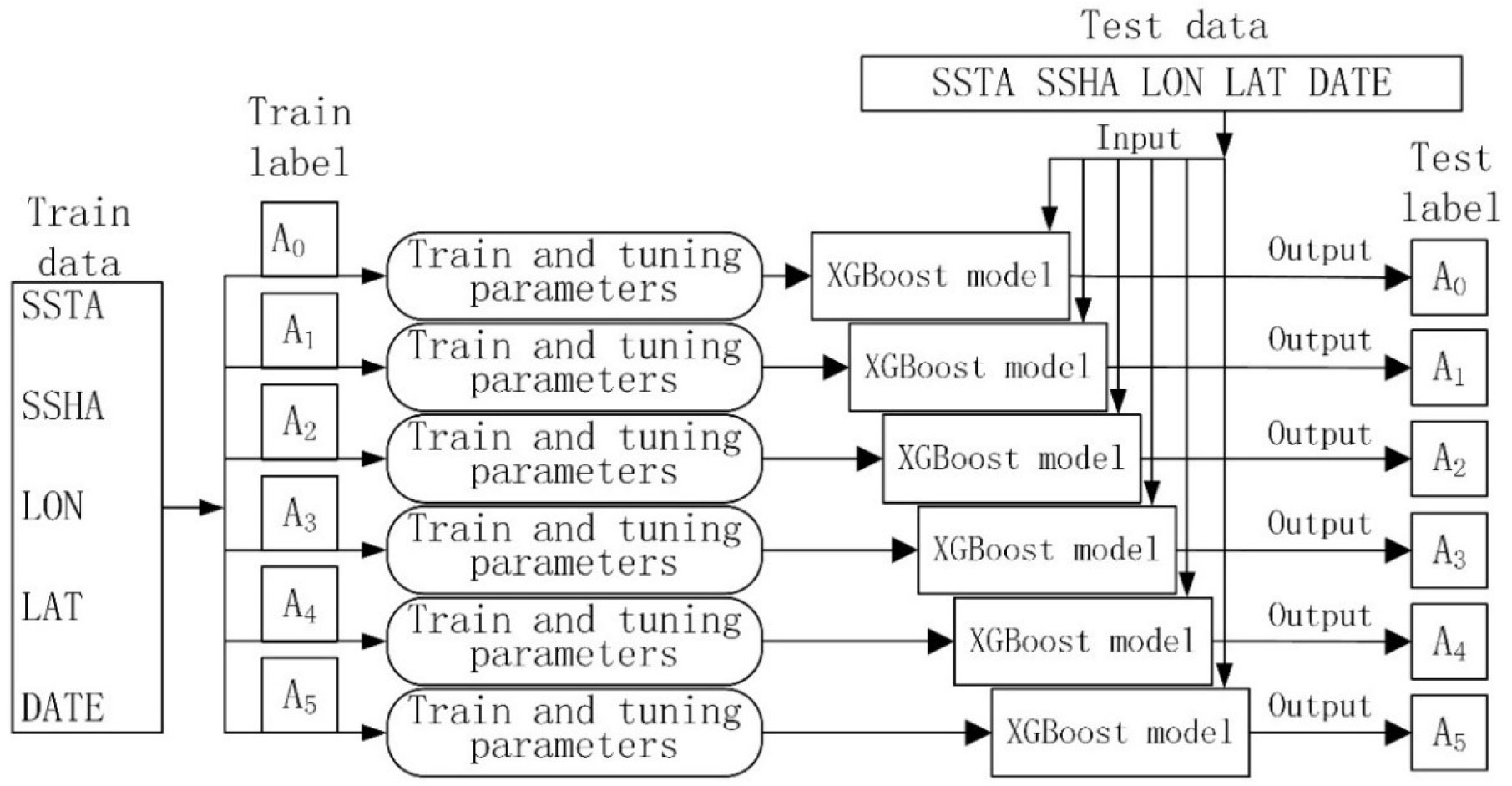
Figure 1 Flow chart of the XGBoost model training and testing.
3. Data
3.1. Satellite remote sensing data
The study used sea surface height data and sea surface temperature data from the 2009–2018 period, which were obtained from the AVISO data center and from daily data sourced at NOAA data centers in the United States, respectively. The time resolution of the above two datasets was 1 day and their spatial resolution was 0.25° × 0.25°.
3.2. Background profile data
The background profile is the constant part in the SSP reconstruction. The background profile comprised climate profile data obtained from the World Ocean Atlas (WOA13) (https://www.nodc.noaa.gov/0C5/woal3/) and it contained the average values of temperature, salinity, and other parameters. This study selected the data of WOA13 in the South China Sea, with a spatial resolution of 1°×1°, were selected.
3.3. Argo data
The Argo data were obtained from the “Global Ocean Argo Scatter Dataset” (ftp://ftp.argo.org.cn/pub/ARGO/global/). All the temperature and salinity profiles measured in the South China Sea from 2009 to 2018 were selected, and the sound speed empirical formula was used to convert the data into the SSP. Interpolate the SSP to the same sampling rate as the background profile.
The areas covering the 12°–20°N and 110°–120°E coordinates in the South China Sea were selected as the inversion regions. The study area has a complex topography, a monsoon climate, and frequent marine activities, such as eddies and internal solitary waves. The combination of these factors challenges the validity of the model. Figure 2A shows the distribution of all samples, amounting to a total of 3881 SSPs. Figure 2B shows the divided training and test data. The profiles from 2009 to 2017 were divided into training data for a total of 3757 items, while the profiles of year 2018 were divided into test data for a total of 124 items.
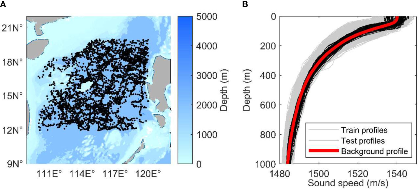
Figure 2 (A) Distribution of the Argo samples in the South China Sea. (B) Training, test, and background profiles.
3.4. EOF analysis
The EOF can describe the perturbation of most SSP features and reduce the dimension of the perturbation of a sample (Carnes et al., 1994). Figure 3 shows the first five modes after EOF normalization, excluding the zero-order mode. From the perspective of the EOF amplitude distribution, the perturbation mainly occurred at a depth of about 100 m, and the perturbation was close to zero at about 1000 m. The samples in the South China Sea are sparse, and the larger the depth, the fewer the samples. Considering the number of samples and EOF perturbation, the research focuses on SSP inversion within 1000 meters.
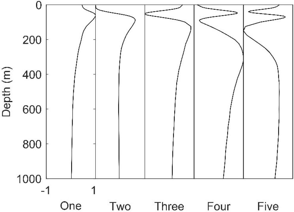
Figure 3 The first five modes of normalized EOF.
Table 1 presents the reconstruction properties of the 1st-to-5th-order EOFs. The contribution rates of these five EOF modes to the variance were 70.72%, 16.24%, 4.67%, 3.30%, and 1.57%, respectively, and the cumulative variance contribution was 96.50%. Although the inversion range was large, there were still several major EOF modes that could describe most of the changes, which confirmed the consistency of the EOF in the South China Sea. The average reconstruction error of the 5th-order EOF was 0.60 m/s, indicating that the reconstruction of this EOF was accurate. Therefore, in the subsequent comparison of the sEOF-r model with the XGBoost model, the SSP was reconstructed using the 5th-order EOF.

Table 1 Variance contribution rate and error of the 1st-to-5th-order EOFs reconstruction.
4. Results and discussion
In this study, the RMSE was used as the precision evaluation index to assess the effect of the two models in the profile inversion in the South China Sea. For the SSP, the RMSE of the XGBoost inversion was 1.75 m/s, and that of the sEOF-r inversion was 2.34 m/s, and the reconstruction accuracy was improved by 25%. Figure 4 shows the error comparison between the sEOF-r and XGBoost models during SSP reconstruction. Except for individual samples, the inversion accuracy of the XGBoost model was significantly better than that of the sEOF-r model. The maximum and average SSP inversion errors produced in the sEOF-r model were 5.02 and 2.21 m/s, respectively, while those produced in the XGBoost model were 3.92 and 1.66 m/s, also respectively. In addition, most of the inversion errors of the XGBoost model were below 1.70 m/s, and their total variance was 0.33 m/s, which was much lower than the value of 0.62 m/s measured in the sEOF-r model. The qualities of robustness and stability were better in the XGBoost than in the sEOF-r model. The latter was obtained by linear fitting based on a large number of samples. This linear relationship represented a statistical result, and it was difficult to deal with samples with large differences between individual and statistical characteristics (Stammer, 1997; Wunsch, 1997). Therefore, the ensemble XGBoost learning algorithm was introduced to eliminate the constraints of linear inversion. In this algorithm, latitude, longitude parameters and time parameters of measuring were introduced to improve the inversion accuracy Especially in samples with large errors, the effect was significant. For example, the maximum error of the XGBoost model inversion was 1.10 m/s smaller than that of the sEOF-r model, and the maximum error of the two models happened to be generated in the same sample. The results showed that the XGBoost model was more suitable than the linear sEOF-r model for defining the complex marine activities of the South China Sea.
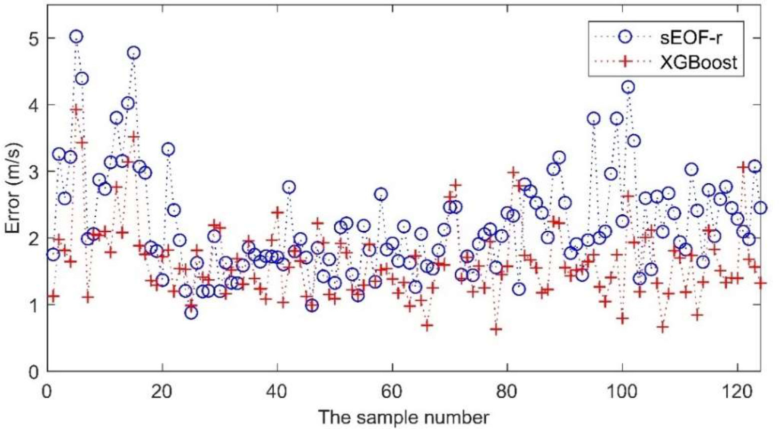
Figure 4 Reconstruction error of two models for different samples.
Figure 5 shows the reconstruction error at different depths. At all depths, the XGBoost model produced smaller errors than the sEOF-r model. For both models, the maximum error was generated at depths close to 100 m, with values of 4.78 m/s for the sEOF-r model and 3.69 m/s for the XGBoost model, which was consistent with the perturbation range of the leading mode in Figure 3. Temperature is the main factor influencing the variation of the speed of sound. Therefore, the sea surface parameters have great influence on the calculation of sea surface sound speed, so the error is small. with large seasonal and diurnal variations in the temperature of the mixed layer, as well as internal solitary waves and other oceanic dynamic activities, leading to the concentration of errors at these depths. When the depth exceeds the mixing layer, the error becomes smaller because the disturbance of the basis function becomes smaller.
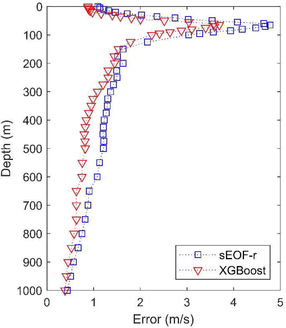
Figure 5 Reconstruction errors of the sEOF-r and XGBoost models at different depths.
Figure 6 shows the first SSP of each month in the reconstructed SSP. The results were consistent with those reported in Figures 4, 5, showing that XGBoost is closer to the measurement profile than the sEOF-r model in almost every sample. This also indicates that the linear model will produce large errors when dealing with numerous samples, especially if containing large differences between individual and statistical characteristics. In the XGBoost model, the simple linear law was broken, and the resulting error was small. Figure 7 shows a comparison of the measured and estimated values of the 0-to-5th-order projection coefficients. Clearly, the ensemble learning model provided better results, and the linear sEOF-r model lagged behind in most cases. As the order increased, the error of the projection coefficient tended to increase. In general, the higher the order, the greater the background noise. Considering the reconstruction accuracy and noise suppression, it is concluded that choosing the 5th-order EOF inversion is sufficient to ensure reconstruction accuracy.
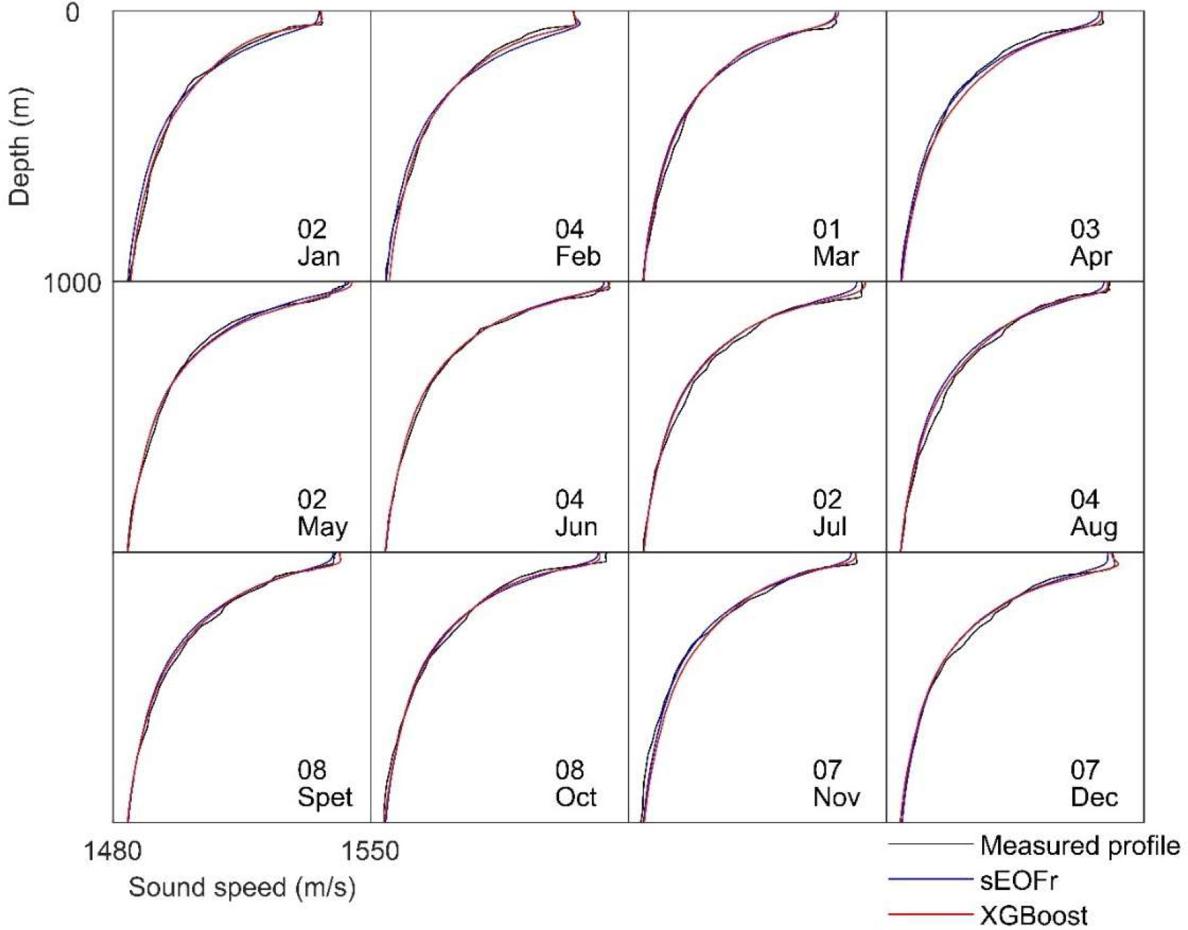
Figure 6 Reconstruction results of the first effective profile for each month.
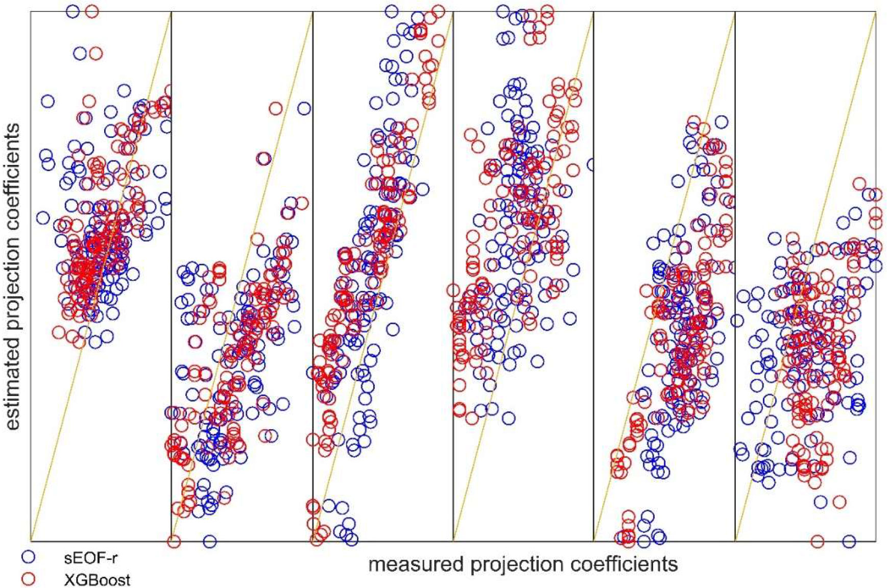
Figure 7 Results of the inversion of the normalized projection coefficients of the first five orders. The straight line indicates perfect inversion. The five orders, from zero to the fifth, are indicated from left to right.
5. Conclusions
The present study proposed a method for reconstructing the SSP based on XGBoost model using SSHA, SSTA, LAT, LON, and DATE as the input data, and the 0-to-5th-order projection coefficients as the output data. Both input and output data were then converted into training data for the 2009–2017 period and test data for 2018 years. The XGBoost model was trained through the training data, and then the test data was used to obtain the SSP’s projection coefficient in 2018. Based on this, the 2018 SSP was inverted, and the RMSE was used as the evaluation metric of the model’s accuracy. The results showed that the RMSE of the XGBoost model was 1.75 m/s, which was 25% less than the 2.34 m/s error detected in the sEOF-r model. Compared with the linear regression model, the XGBoost model showed a better performance. Specifically, it overcame linear constraints, more relevant parameters could be introduced for regression (such as longitude and latitude, measurement date, etc.), there was no analytical restriction, and the relationship between parameters could be more easily discovered. The experiments showed that the XGBoost model had a better and more robust effect than the linear model in the inversion of SSP information.
Data availability statement
The original contributions presented in the study are included in the article/supplementary material. Further inquiries can be directed to the corresponding author.
Author contributions
ZO completed the literature research, analysis, and manuscript writing. KQ completed the Conceptualization, methodology and funding acquisition. MS, YW, and JZ jointly completed the validation, visualization and project administration. All authors contributed to the article and approved the submitted version.
Funding
This research was funded by the Natural Science Foundation of Guangdong Province, grant number No.2022A1515011519.
Conflict of interest
The authors declare that the research was conducted in the absence of any commercial or financial relationships that could be construed as a potential conflict of interest.
Publisher’s note
All claims expressed in this article are solely those of the authors and do not necessarily represent those of their affiliated organizations, or those of the publisher, the editors and the reviewers. Any product that may be evaluated in this article, or claim that may be made by its manufacturer, is not guaranteed or endorsed by the publisher.
References
Bianco M. J., Gerstoft P., Traer J., Ozanich E., Roch M. A., Gannot S., et al. (2019). Machine learning in acoustics: Theory and applications. J. Acoust. Soc Am. 146, 3590–3628. doi: 10.1121/1.5133944
Carnes M. R., Mitchell L., Dewitt P. W. (1990). Synthetic temperature profiles derived from GEOSAT altimetry : comparison with air-dropped expendable bathythermograph profiles. J. Geophys. Res. Atmos. 95, 17979–17992. doi: 10.1029/JC095iC10p17979
Carnes M. R., Teague W. J., Mitchell J. L. (1994). Inference of subsurface thermohaline structure from fields measurable by satellite. J. Atmos. Ocean. Technol. 11, 551–566. doi: 10.1175/1520-0426(1994)011<0551
Carroll P., Mahmood K., Zhou S., Zhou H., Xu X., Cui J.-H. (2014). On-demand asynchronous localization for underwater sensor networks. IEEE Trans. Signal Process. 62, 3337–3348. doi: 10.1109/TSP.2014.2326996
Cheng L., Ji X., Zhao H., Li J., Xu W., et al. (2022). Tensor-based basis function learning for three-dimensional sound speed fields. J. Acoustical Soc. America 151, 269. doi: 10.1121/10.0009280
Chen T., Guestrin C. (2016). XGBoost: A scalable tree boosting system. ACM, 785–794. doi: 10.1145/2939672.2939785
Chen C., Ma Y., Liu Y. (2018). Reconstructing sound speed profiles worldwide with sea surface data. Appl. Ocean Res. 77, 26–33. doi: 10.1016/j.apor.2018.05.002
Chen C., Yan F., Gao Y. A., Jin T., Zhou Z. (2020). Improving reconstruction of sound speed profiles using a self-organizing map method with multi-source observations. Remote Sens. Lett. 11:6, 572–580. doi: 10.1080/2150704X.2020.1742940
Erol-Kantarci M., Mouftah H. T., Oktug S. (2011). A survey of architectures and localization techniques for underwater acoustic sensor networks. IEEE Commun. Surv. Tut. 13, 487–502. doi: 10.1109/SURV.2011.020211.00035
Fox D. N., Teague W. J., Barron C. N., Carnes M. R., Lee C. M. (2002). The modular ocean data assimilation system (MODAS). J. Atmos. Ocean. Technol. 19, 240–252. doi: 10.1175/1520-0426(2002)019<0240
Isik M. T., Akan O. B. (2009). A three dimensional localization algorithm for underwater acoustic sensor networks. IEEE Trans. Wirel. Commun. 8, 4457–4463. doi: 10.1109/TWC.2009.081628
Klemas V., Yan X. H. (2014). Subsurface and deeper ocean remote sensing from satellites: An overview and new results. Prog. Oceanogr. 122, 1–9. doi: 10.1016/j.pocean.2013.11.010
Kundu P. K., Allen J. S., Smith R. L. (1975). Modal decomposition of thevelocity field near the Oregon coast. J.Phys.Oceanogr. 5, 683–704. doi: 10.1175/1520-0485(1975)005<0683:MDOTVF>2.0.CO;2
Leblanc L. R., Middleton F. H. (1980). An underwater acoustic sound velocity data model. J. Acoust. Soc Am. 67, 2055–2062. doi: 10.1121/1.384448
Li Y., Gao P., Tang B., Yi Y., Zhang J. (2022). Double feature extraction method of ship-radiated noise signal based on slope entropy and permutation entropy. Entropy 24, 22. doi: 10.3390/e24010022
Li Y., Geng B., Jiao S. (2022). Dispersion entropy-based lempel-ziv complexity: A new metric for signal analysis. Chaos Solitons Fractals. 161, 112400. doi: 10.1016/j.chaos.2022.112400
Li H., Qu K., Zhou J. (2021). Reconstructing sound speed profile from remote sensing data: Nonlinear inversion based on self-organizing map. IEEE Access 9, 109754–109762. doi: 10.1109/ACCESS.2021.3102608
Li Q., Shi J., Li Z., Luo Y., Yang F., Zhang K., et al. (2019). Acoustic sound speed profile inversion based on orthogonal matching pursuit. Acta Oceanol. Sin. 38, 149–157. doi: 10.1007/s13131-019-1505-4
Li W., Su H., Wang X., Yan X. H. (2017). Estimation of global subsurface temperature anomaly based on multisource satellite observations. J. Remote. Sens. 21, 881–891. doi: 10.11834/jrs.20177026
Li Y., Tang B., Yi Y. (2022). A novel complexity-based mode feature representation for feature extraction of ship-radiated noise using VMD and slope entropy. Appl. Acoustics. 196, 108899. doi: 10.1016/j.apacoust.2022.108899
Liu J., Wang Z., Cui J.-H., Zhou S., Yang B. (2016). A joint time synchronization and localization design for mobile underwater sensor networks. IEEE Trans. Mob. Comput. 15, 530–543. doi: 10.1109/TMC.2015.2410777
Pauthenet E., Roquet F., Madec G., Nerini D. (2017). A linear decomposition of the southern ocean thermohaline structure. J. Phys. Oceanogr. 47, 27–47. doi: 10.1175/JPO-D-16-0083.1
Stammer D. (1997). Global characteristics of ocean variability estimated from regional TOPEX/POSEIDON altimeter measurements. J. Phys. Oceanogr. 27, 1743–1769. doi: 10.1175/1520-0485(1997)027<1743
Su H., Wu X., Yan X. H., Kidwell A. (2015). Estimation of subsurface temperature anomaly in the Indian ocean during recent global surface warming hiatus from satellite measurements: A support vector machine approach. Remote Sens. Environ. 160, 63–71. doi: 10.1016/j.rse.2015.01.001
Teymorian A. Y., Cheng W., Ma L., Cheng X., Lu X., Lu Z. (2009). 3D underwater sensor network localization. IEEE Trans. Mob. Comput. 8, 1610–1621. doi: 10.1109/TMC.2009.80
Tolstoy A., Diachok O., Frazer L. N. (1991). Acoustic tomography via matched field processing. J.Acoust. Soc.Am. 89, 1119–1127. doi: 10.1121/1.400647
Keywords: sound speed profile, remote sensing data, XGBoost, Argo profiles, the South China Sea
Citation: Ou Z, Qu K, Shi M, Wang Y and Zhou J (2022) Estimation of sound speed profiles based on remote sensing parameters using a scalable end-to-end tree boosting model. Front. Mar. Sci. 9:1051820. doi: 10.3389/fmars.2022.1051820
Received: 26 September 2022; Accepted: 25 November 2022;
Published: 08 December 2022.
Edited by:
Yuxing Li, Xi’an University of Technology, ChinaReviewed by:
Yang Xuefeng, Institute of Acoustics (CAS), ChinaXiaoman Li, Jiangsu University of Science and Technology, China
Copyright © 2022 Ou, Qu, Shi, Wang and Zhou. This is an open-access article distributed under the terms of the Creative Commons Attribution License (CC BY). The use, distribution or reproduction in other forums is permitted, provided the original author(s) and the copyright owner(s) are credited and that the original publication in this journal is cited, in accordance with accepted academic practice. No use, distribution or reproduction is permitted which does not comply with these terms.
*Correspondence: Ke Qu, cXVrZUBnZG91LmVkdS5jbg==