Assessment of CO2 and O2 spatial variability in an indigenous aquaculture system for restoration impacts

Spatial variability in carbon dioxide (CO₂) and oxygen (O₂) was assessed within an Indigenous Hawaiian fishpond undergoing active ecosystem restoration. The brackish, tidal fishpond is located within Kāne‘ohe Bay, Hawai‘i. Following a year of monthly discrete sampling, a significant shift in DIC and percent O₂ saturation was observed along the North-South axis within the pond. The south end of the pond was higher in DIC (+35 μmol·kg⁻¹) and lower in percent O₂ saturation (-19%) than the north end, which exhibited values similar to those observed in water entering the fishpond from the bay. Water quality parameters and inequal proximity to water flux sites suggested that a difference in residence time may exist along the north-south axis. In addition, ΔTA/ΔDIC relationships revealed a respiration signal in south end of the pond, which was enhanced at depth. While physical processes strongly affect CO₂ and O₂ across various temporal scales, spatial patterns in biological processes may also affect variability within the fishpond. These findings demonstrate that changes in water chemistry within the fishpond are the result of ecosystem restoration efforts. In turn, future management decisions at the fishpond will play an important role in preserving its viability as a healthy habitat for the intended marine species.

1 Introduction

A steady increase in atmospheric carbon dioxide (CO₂) and decrease in global dissolved oxygen (DO) in the open ocean have had profound effects on the chemistry of ocean waters (e.g., Bacastow and Keeling, 1973; Riebsell et al., 2000; Brix et al., 2004; Andersson, 2005; Dore et al., 2009; Goodwin & Lauderdale, 2013; Breitburg et al., 2018). Uptake of elevated atmospheric CO₂ into seawater leads to the formation of carbonic acid in a process known as ocean acidification (e.g., Caldeira & Wickett, 2003; Orr et al., 2005; Cao et al., 2014; Ono et al., 2019), while the decline in DO creates new stressors for ocean life and ecosystems as oxygen becomes less biologically available (e.g., Breitburg et al., 2018). To date, much of the focus on these topics has been oriented towards large-scale patterns and processes in the open ocean. However, the prioritization of sustainable coastal development has created new interest in coastal and estuarine systems. Wetlands and flooded-field ecosystems, often found within estuarine spaces, occupy a critical boundary between land and sea, where the concentration of natural and anthropogenic activity can give rise to spatially confined changes in coastal chemistry that deviate from broader global trends, such as coastal acidification (Rixen et al., 2015; Chan et al., 2017; Hall et al., 2020) coastal deoxygenation (Rixen et al., 2015; Bednaršek et al., 2016; Feely et al., 2017) and eutrophication (Flynn et al., 2015; Laurent et al., 2017). Importantly, this space hosts aquatic life of immense biodiversity and productivity, while also serving as a major focus of human development and activity (Andersson, 2005; Doney et al., 2020; Jokiel et al., 2011).

Serving as an exemplar of sustainable bioengineering in estuarine environments, Native Hawaiians recognized the immense potential for productivity in estuaries and utilized this setting for Indigenous aquaculture systems, or loko i‘a (Kikuchi, 1976; Keala et al., 2007). Loko i‘a are often built-in areas that represent the brackish mixing zone of the ahupua‘a, a Native Hawaiian social-ecological land and water management system. In this system, stream water collects and transports organic matter and nutrients as it runs through the watershed and through agro-ecological systems, such as lo‘i, which are flooded-field wetlands with taro that provide nutritive sustenance as well as habitat for native fauna (Winter et al., 2018). The lo‘i system results in increased ecosystem services, whic include habitat for native flora and fauna as well as serving as sediment retention basins (Koshiba et al., 2013; Bremer et al., 2018; Winter et al., 2020a). Likewise, high nutrient streamflow and groundwater discharge is consumed for primary production within the coastal fishpond, which is situated landward of the reef, thereby promoting healthy nearshore reef communities (Winter et al., 2018). The locations of loko i‘a thus represented deep ecological and biogeochemical understanding of the seasonal and spatial patterns of the landscape by Indigenous Hawaiians, such as land-based (Ringuet and Mackenzie, 2007; De Carlo et al., 2007) and groundwater (Kleven et al., 2014; Dulai et al., 2016) input of nutrients into coastal regions, as well as the biological response and subsequent effects on estuarine and marine food webs. In this way, loko i‘a were continuously maintained for hundreds of years and provided a resilient, reliable source of food, such as herbivorous fish and macroalgae for Hawaiian communities (Maly and Maly, 2003; Demopoulos et al., 2007).

The functioning of the ahupua‘a system of watershed management was upended in the post contact period of Hawaiian history, as plantation-based agriculture supplanted community-based subsistence farming (Camvel, 2020). The current restoration of a loko i‘a presents an opportunity to quantitatively study what Native Hawaiians likely knew empirically about maintaining a biogeochemical balance in the fishponds. Analysis of restoration efforts will both further the understanding of historic fishpond use and provide insight into the future stability of long-term agro-ecological systems.

Prior research at the study site (Drupp et al., 2011; D'Andrea et al., 2015; Drupp et al., 2016; McCoy et al., 2017) has correlated past incidents of hypoxia and fish mortality with physical processes, such as wind strength and thermal stress. Efforts to better manage aquaculture resources and safeguard the health of cultivated species are likely to benefit from this baseline assessment. CO₂ and O₂ respond to a wide range of biogeochemical processes, making them useful indicators for understanding ecosystem change. As such, a baseline dataset of CO₂ and O₂ variability will be a valuable tool to support management of fishpond for both planning further restoration and anticipating ecosystem response to climate change.

The work presented here aims to expand the understanding of Hawaiian loko i‘a by characterizing the concentrations of carbonate parameters and DO, allowing us to assess the balance of production and respiration within Indigenous resource management systems. The initiation of this study follows a large-scale invasive plant species removal effort and will provide insight into the effects of this aspect of restoration and ecosystem management.

2 Study area

Loko I‘a o He‘eia is located on the windward side of O‘ahu along the western side of Kāne‘ohe Bay. The ambient temperature in Kāne‘ohe varies between 28.17-21.78 °C during the year. Likewise, the bay experiences average annual precipitation of 136.65 cm (Western Regional Climate Center, Kāne‘ohe Station 838.1, 1905-2016). Kāne‘ohe Bay typically experiences mixed semi-diurnal tides with a mean tidal height of 0.36 m ( ± 0.29 m) (Young, 2011). The fishpond itself is part of the broader He‘eia ahupua‘a (Figure 1) that includes the land, streams, and the offshore reef systems. A portion of the He‘eia ahupua‘a was designated as the 29th National Estuarine Research Reserve (NERR) in 2017, with restoration of Indigenous resource management systems as one of its main goals (Winter et al., 2020b). One of the main efforts undertaken to restore Indigenous agro-ecological systems such as lo‘i and loko i‘a has been the removal of invasive species, including invasive mangroves such as Rhizophora mangle, and invasive algae, such as Gracilaria salicornia and Acanthophora spicifera. In He‘eia, introduction and proliferation of invasive mangroves built up a thick bank of organic rich sediment around the landward pond perimeter, restricting stream flow into the fishpond. The subsequent removal of these mangroves has resulted in elevated fresh water supply, decreasing fishpond salinity and temperature, as well as increasing dissolved oxygen over the last decade of restoration work. (Leon Soon, 2017; McCoy et al., 2017; Möhlenkamp et al., 2019; Lopera, 2020).

FIGURE 1

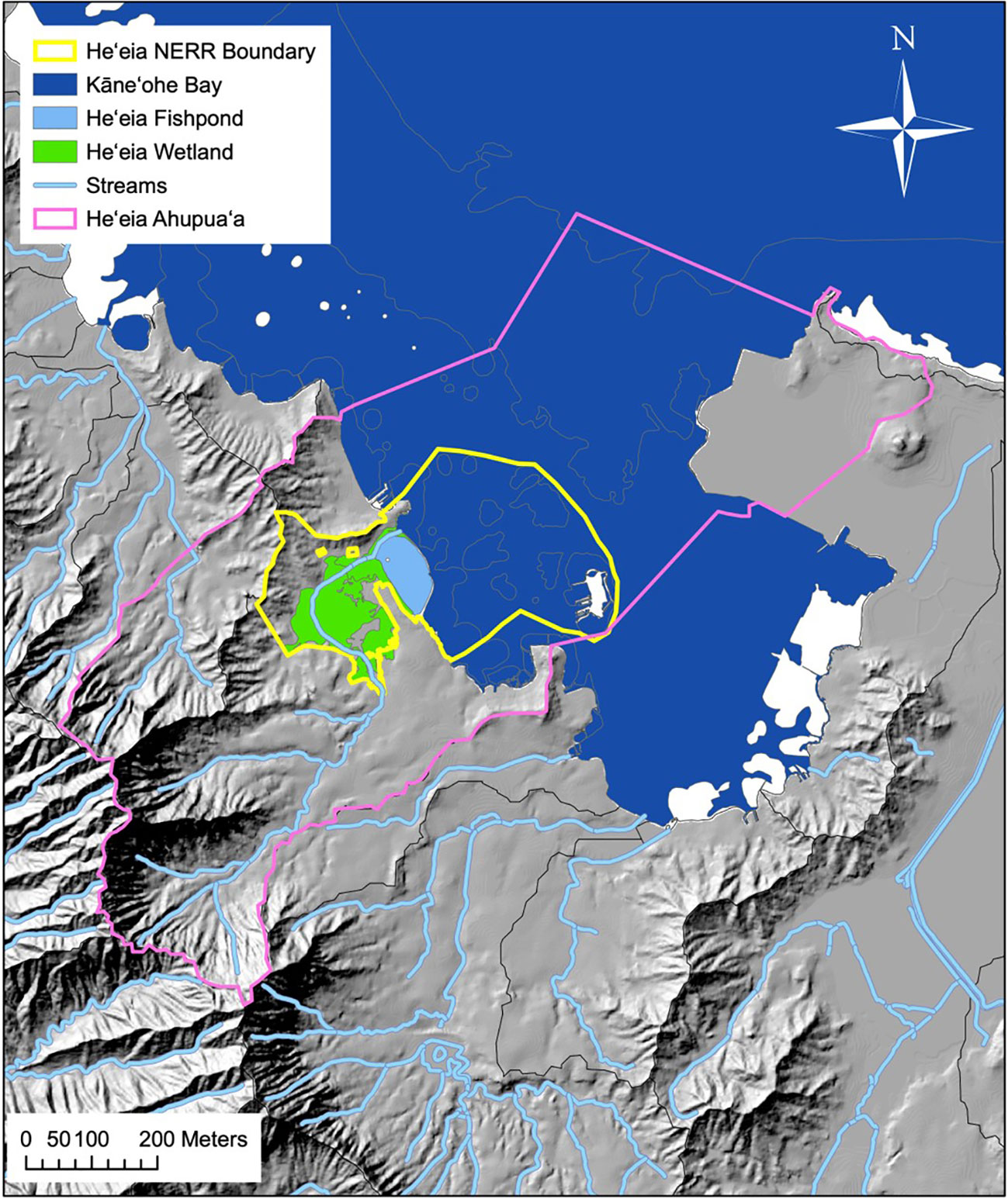
Figure 1 He‘eia ahupua‘a, Ko‘olaupoko, O‘ahu. Solid orange line represents ahupua‘a boundaries in the Hawai‘i Statewide GIS Program, with lines extended to include the approximately represented historical He‘eia fishery following the ahupua‘a of He‘eia land commission award (L.C.Aw.10613, Ap.1 to A. Paki. From Public archives of Hawai‘i, Letter Folder 244-B, H.A. & R.L. 3/3/47). Map credit: He‘eia NERR.

He‘eia Fishpond (Figure 2) is a 0.356 km² embayment enclosed by approximately 2.5 km of basalt and coral rubble wall. Along this wall are seven sluice gates, called mākāhā, which allow for tidally influenced flow of water into and out of the fishpond. There are four mākāhā along the seaward wall (Figure 2, 15, 17-19), allowing for water exchange from Kāne‘ohe bay, and three mākāhā along He‘eia Stream (Figure 2, 12 &13) allowing for fresh/brackish water exchange. Brackish water forms a gradient, running along the landward edge of the pond from the freshwater stream mākāhā in the north, towards the south end of the pond. The fishpond has an average depth of 0.7 m but is not uniform, being generally shallower at the southern end of the fishpond and deeper at the north end and at each of the mākāhā (Yang, 2000; Young, 2011). The remains of a mangrove island removed during a previous phase of restoration (2018-2019) are situated near the stream mākāhā in the north and cause the pond bathymetry to shoal around it. The fishpond interior sits on a fossilized reef previously covered in sand and coral debris. There has been an increase in land derived organic-rich sediments over the last century however, as a result of land use changes upstream. (Costa-Pierce, 1987)

FIGURE 2

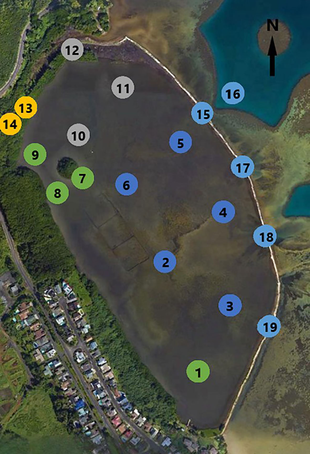
Figure 2 He’eia Fishpond, sampling locations numbered: in pond 1-11; Stream facing mākāhā 12 & 13; Ocean facing mākāhā 15, 17, 18, 19; Stream and Ocean endmembers 14 & 16. Station color matches spatial groupings identified in Figure 3. (Image from Google Earth modified by Evan Lechner).

3 Materials/methods

3.1 Sampling frequency and sites

Sampling was conducted (Summarized Table 1) on a monthly basis between August 2019-August 2020. Fieldwork was timed to occur across a neap low tide each month to minimize the potential effect of tidal variability during the course of the sampling day (Young, 2011). Likewise, sampling was conducted over the same early morning period to minimize the effect of diurnal variability.

TABLE 1

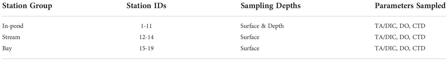
Table 1 Station groups by geographic location with referenced station IDs, sampled depths, and measured parameters.

A sampling grid (Figure 2) was chosen to line up with past field campaigns and build upon an existing library of overlapping measurements (Young, 2011; Dulai et al., 2016; Möhlenkamp et al., 2018; Lopera, 2020). In-pond samples were taken at 11 separate stations, numbered 1-11. Sampling was also conducted at 6 of the 7 mākāhā, including 2 stream-facing mākāhā (12, 14) and 4 bay-facing mākāhā (15, 17, 18, 19). A 7^th mākāhā, a stream-facing mākāhā near station 9, was not included in the sampling plan because it was constructed near the end of the project. Lastly, endmember reference samples were collected, with the freshwater endmember (14) collected from He‘eia Stream just stream-ward of 13, and the ocean endmember (16) collected from Kāne‘ohe Bay several meters beyond bay-facing mākāhā 15.

At each of the in-pond stations, sampling was conducted at two depths for all sampled parameters. One sample was collected from 5-10 cm below the air-sea interface, and a second was collected from 5-10 cm above the pond bottom. All samples were performed manually, using a 0.5 m length of tubing to prevent excess bubbles from altering the composition of sampled water. For all 6 mākāhā stations and the 2 endmember stations a single sample was collected 5-10 cm below the air-sea interface. The operating assumption was that the mākāhā stations were well mixed due to the vigorous nature of water flowing through the sluice gates.

3.2 Sample collection

Samples for analysis of Totally Alkalinity (TA) and Dissolved Inorganic Carbon (DIC) were collected in 250 mL Biological Oxygen Demand (BOD) bottles, while samples were collected for Dissolved Oxygen (DO) analysis using volumetrically calibrated 60mL BOD bottles. Replicate samples were taken for surface and depth at 1-2 sites per trip on a randomized, rotating basis.

All bottles used for sampling were soap and water washed prior to each field visit. Additionally, bottles for TA/DIC were combusted (550 °C) after washing to incinerate any remaining organic material.

During sample collection, each bottle was rinsed three times with ambient water from the depth being sampled. TA/DIC samples were poisoned with 200 μL of HgCl₂ and sealed with Apezion grease to preserve gas composition within the sample and headspace. Likewise, DO samples were subjected to the Winkler method (Codispoti, 2001), in which manganous chloride (MnCl₂), sodium hydroxide (NaOH), and sodium iodide (NaI) were added to the sample to precipitate dissolved oxygen in the form of a tetravalent oxide of manganese (2MnO(OH) ₂). Once treated, samples were stored in a light-proof box until returned to the lab for analysis. All samples were stored in the dark at lab room temperature (~20 °C). DO samples were analyzed within a maximum of 48 hours, while TA/DIC samples were analyzed within a maximum of one month.

Casts were conducted for measurements of conductivity, temperature, and depth using a 10 m range Van Essen CTD Diver (Model# DI281) in tandem with the carbon parameter sample collections at a 10 second measurement frequency for a duration of approximately 120 seconds at the sampled depth. Mean salinity and temperature values were determined from the data set of CTD measurements at each station and at each depth.

Weather data was collected from the HIMB Weather Station at Moku o Lo‘e (Rodgers et al., 2005). Mean He‘eia streamflow data was approximated using data from the Ha‘ikū Stream Gauge (USGS Station #16275000).

3.2.1 Tidal variability measurements

Additional sampling was conducted during the month of July 2020 in order to highlight the relative effect of tidal variability at the study site. Sampling occurred at times targeting both the usual neap tide (7/11/2020), as well as a spring tide (7/04/2020), to examine the range of variability between the two tidal extremes. This timing was particularly advantageous, as the 7/04/2020 spring tide was also the king tide for the year (University of Hawaii Sea Grant, 2018), allowing for examination of the maximum tidal variability at the site. Sampling followed the previously described methodology and samples were collected consistent with the stations and depths sampled throughout the rest of the project. While the results of this tidal sampling campaign are not included here, the sampling plan was a critical step in isolating the various forms of temporal and spatial variability that were expected to influence measurements at He‘eia. While tidal variability was found to be significant at He‘eia, the results demonstrated the selected neap tide sampling was effective at minimizing the effect of tidal change.

3.2.2 Diurnal variability measurements

Two neap tide sampling dates were selected during August 2020 for a diurnal study. For the first neap tide (8/11/2020), two sampling trips were conducted over a 24-hour period to examine the extent of day/night variability. The sampling times of 2am and 2pm were selected to capture peak respiration and peak photosynthesis recorded in the bay, respectively (Shamberger et al., 2011). The date for this experiment was chosen because the pond experienced a weak diurnal tide, rather than the usual mixed semi-diurnal. Targeting an unusually weak neap tide for this experiment limited the effects of tidal variability during sampling.

For this experiment a narrowed sampling grid was adopted in order to complete the sampling run over a shorter 1–2 hour window, allowing for a more accurate representation of the timed peaks in photosynthesis and respiration. Eight in-pond sites (1, 2, 3, 4, 5, 6, 8, 11) were selected and sampled at surface and depth. In selecting these sites, special consideration was made to cover a wide spatial range, while still capturing the typical mixing gradients observed during this and previous field campaigns. Just as with the tidal variability results, the results of the diel variability are not included here. The observation of potential diel variability was needed in order to appropriately contextualize any spatial variability within diel cycles in ecosystem production and respiration.

3.3 Water sample analysis

3.3.1 Carbon parameters

All carbon analyses followed the best practices guide (Dickson et al., 2007) and were validated using Certified Materials (Dickson, 2001). TA and DIC analyses were conducted with a standard accuracy of ± 2 μmol·kg^-1 (Knor et al., 2018).

TA samples were analyzed with an automated open-cell acid-base titration system designed by Dr. Andrew Dickson for high-precision GO-SHIP measurements (personal communication, 2018). Titrations were conducted using an 876 Dosimat Metrohm Plus, an Agilent 34970A Data Acquisition Unit, and a Sierra SmartTrack 50 Mass Flow Controller. Auto-titration was controlled via the Alkalinity 2.9j program (Dickson personal communication, 2018).

DIC samples were analyzed on an Apollo DIC Analyzer (Model AS-C3). Sample temperature was taken immediately prior to analysis via Fluke 51ii Digital Thermometer.

The results of TA & DIC analyses were entered into the CO2Sys program v2.5 (Pierrot et al., 2006) to determine the other two carbon parameters pCO₂ and pH, allowing the carbon system to be fully described. Due to the large salinity range observed at the study site, the dissociation constants defined by Cai and Wang (1998) were selected, which particularly focused on the salinity ranges typically observed in estuaries. Constraining the carbon system in this way also allowed for the derivation of other parameters, such as the saturation state of aragonite, Ω_Ar. In addition to the derivation of these additional parameters, the uncertainty of each parameter was also calculated. pCO₂ was calculated as having an uncertainty of ±9.82 μatm, pH uncertainty was ±0.01, and Ω_Ar ± 0.16.

3.3.2 Dissolved oxygen

Analyses of DO samples were conducted via Modified Winkler Titration as described by Codispoti (2001). Preserved samples were acidified with sulfuric acid (28% v/v) to convert manganic hydroxide to manganic sulfate and were then titrated with sodium thiosulfate. Standardization of sodium thiosulfate titrant was conducted for each round of sampling using a 0.1 N Potassium Iodate standard as described in Codispoti (2001). Dissolved oxygen data was subsequently combined with collected temperature and salinity data to derive the percent oxygen saturation for the sample (Benson and Krause, 1980; Benson and Krause, 1984; U.S. Geological Survey, 2011). Dissolved oxygen analyses were conducted with a standard accuracy of 0.19%, typical of the normal range 0.1% - 0.3% (Carpenter, 1965; Codispoti, 2001; Wong, 2012).

4 Results

4.1 Spatial survey

Organizing salinity data by stations (Figure 3), the estuary was divided into three identifiable water types. The first was a relatively uniform seawater source (33.73, 2σ=1.08) derived from Kāne‘ohe Bay. This salinity characterizes the four ocean mākāhā and the ocean endmember, stations 15-19. Similarly, there was a uniform fresh-water source (0.29, 2σ=0.32) fed by He‘eia Stream, represented by the upstream freshwater mākāhā and the stream endmember, stations 13 & 14. Lastly, the pond interior was treated as a non-uniform brackish mixture (29.45, 2σ=1.79) of the two previously described water types. Stations 1-11 covered the pond interior, while 12, despite being a mākāhā, was included in the brackish category as well. Due to its position at the mouth of He‘eia stream, 12 exhibited salinities that more closely resembled the conditions within the pond, rather than the conditions of either of the source water types.

FIGURE 3

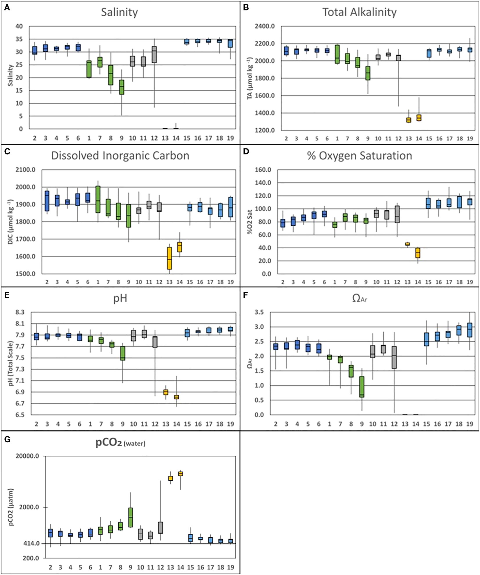
Figure 3 Vertically and temporally averaged data [(A)Salinity; (B)Total Alkalinity; (C) Dissolved Organic Carbon; (D) % O₂ Saturation; (E) pH; (F) Ω_Ar (G) pCO_2(water)] separated by sampling stations and organized into the designated spatial groups: Pond Center (Dark Blue: Stations 2-6); Fresh Water Lens (Green: Stations 1, 7, 8 & 9); North Pond (Gray: Stations 10, 11 & 12); Stream Water Source (Yellow: Stations 13 & 14); Bay Water Source (Light Blue: Stations 15-19).

Baseline temporal variability observed during the field campaign was largely connected to the arrival of the wet season in January and February. Salinity was observed to vary by 8.73 was observed between October (34.36) and January (25.63). TA varied by 173.3 μmol·kg⁻¹ over this same period between a high of 2141.2 μmol·kg⁻¹ and a low of 1967.9 μmol·kg⁻¹. Temporal variability in DIC was 142.2 μmol·kg⁻¹ between the October high (1984.9) and the January low (1842.7). Oxygen variability presented an inversed temporal pattern, varying by 27.02% between an October low (67.19%) and a February high (94.21%). The temporal variability in pH was 0.22, while Ω_Ar varied by 0.86.

4.2 Salinity

The collected salinity data (Figure 3A) further revealed three spatial zones within the pond. Stations 2-6, located at the center of the pond, are in the closest proximity to the bay-facing mākāhā. Averaged together these stations exhibited a mean salinity of 32.87 (2σ=0.97) varying between 32.23 (2σ=1.53) at the surface and 33.51 (2σ=1.12) at depth. Stations 10 & 11 were positioned furthest to the north in the pond adjacent to both stream and bay-facing mākāhā. These stations were fresher with a mean salinity of 28.58 (2σ=3.20) varying between 28.88 (2σ=2.51) at the surface and 29.01 (2σ=3.55) at depth. Lastly, stations 1 & 7-9 were closest to land, and displayed a freshwater lens running north to south from station 9 towards station 1. The mean salinity across this gradient was 25.42 (2σ=2.65) varying between 23.47 (2σ=3.93) at the surface and 27.58 (2σ=2.65) at depth.

4.3 Total alkalinity

Within the pond, TA (Figure 3B) followed a distribution similar to salinity. Stations 2-6 exhibited a mean alkalinity of 2119.1 μmol·kg⁻¹ (2σ=20.3) varying between 2115.6 μmol·kg⁻¹ (2σ=30.8) at the surface and 2122.5 μmol·kg⁻¹ (2σ= 27.8) at depth. Stations 10 & 11 were characterized by a mean alkalinity of 2037.5 μmol·kg⁻¹ (2σ=60.5) varying between 2056.4 μmol·kg⁻¹ (2σ=35.3) at the surface and 2067.5 μmol·kg⁻¹ (2σ=35.3) at depth. Lastly, the mean alkalinity across the gradient comprised of stations 1 & 7-9 was 1977.5 μmol·kg⁻¹ (2σ=60.8), varying between 1937.2 μmol·kg⁻¹ (2σ=67.2) at the surface and 2021.4 μmol·kg⁻¹ (2σ=67.4) at depth.

4.4 Dissolved inorganic carbon

The distribution of DIC (Figure 3C) differed from the pattern observed in salinity and TA. Stations 2-6 exhibited the highest concentrations with a mean DIC of 1924.0 μmol·kg⁻¹ (2σ=24.3), varying between 1924.5 μmol·kg⁻¹ (2σ=35.9) at the surface and 1923.6 μmol·kg⁻¹ (2σ=34.3) at depth. Stations 10 & 11 had a lower mean DIC at 1876.4 μmol·kg⁻¹ (2σ=32.8), varying between 1883.5 μmol·kg⁻¹ (2σ=38.2) at the surface and 1883.8 μmol·kg⁻¹ (2σ=34.0) at depth. DIC concentration at Stations 1 & 7-9 was similar to that observed at Stations 10 & 11, with the mean value across this gradient of 1878.0 μmol·kg⁻¹ (2σ=41.4), varying between 1861.0 μmol·kg⁻¹ (2σ=67.2) at the surface and 1896.7 μmol·kg⁻¹ (2σ=46.4) at depth.

4.5 %Oxygen saturation

The % oxygen saturation data (Figure 3D) shows an inverse pattern with respect to DIC. The three main macroscale water types (the bay, the stream, and the in-pond) remained distinct. The highest % saturation values were observed in the bay sourced waters, where all sampling sites were supersaturated with respect to oxygen. On the other end, the lowest % saturation values were observed in the stream source waters. Within the pond, %O₂ varied between these two extremes.

Stations 2-6 exhibited a mean %O₂ of 84.91% (2σ=5.09) varying between 84.39% (2σ=7.36) at the surface and 85.44% (2σ=7.35) at depth. Mean %O₂ at Stations 10 & 11 was 90.21% (2σ=7.83) varying between 90.64% (2σ=8.33) at the surface and 92.34% (2σ=8.86) at depth. The North-South gradient across stations 1 & 7-9 displayed a mean %O₂ of 80.86% (2σ=5.84) varying between 82.64% (2σ=8.38) at the surface and 78.93% (2σ=8.28) at depth.

The in-pond percent oxygen saturation data significantly builds upon previously described North-South patterns. In general, landward-seaward position within the fishpond seem to affect the measured oxygen saturation, with lower values observed among the more landward stations (1, 2, 8 & 9; mean O₂ = 78.9% ± 12.1) while higher values were observed among the more seaward stations (4, 5, 6, 7; mean O₂ = 87.9% ± 11.2).

4.6 pCO2_(water)

pCO₂ data derived from discrete sampling of TA and DIC demonstrated a pattern in spatial variability between station groups that follows the trend in mixing of bay and stream derived waters outlined in the salinity data. The highest pCO₂ (Figure 3G) values were observed in the stream where the mean value between stations 13 & 14 was 7994.1 μatm (2σ=1551.9). The lowest values were observed in Kāne‘ohe Bay & mākāhā stations (15-19) where the mean value was 477.7 μatm (2σ=57.2). Station groups within the pond varied in pCO₂ values but were within the high and low extremes exhibited by the stream and bay water sources. The center of the pond (stations 2-6) exhibited a mean pCO₂ of 605.5 μatm (2σ=85.3). The mean pCO₂ in the north of the pond (stations 10 & 11) 845.0 μatm (2σ=505.8). Meanwhile, the south of the pond (stations 1 & 7-9) was observed to have a mean pCO₂ of 997.9 μatm (2σ=293.0).

4.7 pH

The subdivided spatial regime that has been outlined in the data examined so far also applies to the other measured parameters of the constrained carbon system. Looking to the spatial variability of pH (Figure 3E), ocean source waters maintained a relatively uniform pH of 7.97 (2σ=0.04), with a slight trend towards higher pH in stations further south. In the same vein, the stream waters were a distinct and separate source, providing weakly acidified water (pH 6.87; 2σ=0.10) to the estuary.

Stations 2-6 exhibited a mean pH of 7.89 (2σ=0.04) varying between 7.89 (2σ=0.06) at the surface and 7.88 (2σ=0.05) at depth. Stations 10 & 11 had a mean pH of 7.84 (2σ=0.11) varying between 7.89 (2σ=0.06) at the surface and 7.91 (2σ=0.07) at depth. Lastly, the North-South gradient across stations 1 & 7-9 held a mean pH across this gradient was 7.71 (2σ=0.08) varying between 7.67 (2σ=0.11) at the surface and 7.76 (2σ=0.09) at depth. The in-pond pH data resembles the distribution visible in salinity and TA, in which the largest variability is associated with the North-South freshwater gradient running from station 9 to station 1.

4.8 Ω_Ar

Aragonite saturation state was observed highest closest to the bay. Likewise, the stream source waters were extremely undersaturated with respect to aragonite, consistent with the acidic conditions reported by the pH data. The undersaturation carried over to in-pond conditions as well, with station 9 presenting a slight undersaturation with respect to aragonite as well.

In the Ω_Ar data set (Figure 3F) Stations 2-6 exhibited a mean Ω_Ar of 2.28 (2σ=0.13) varying between 2.25 (2σ=0.19) at the surface and 2.30 (2σ=0.18) at depth. Mean Ω_Ar Stations 10 & 11 was 2.09 (2σ=0.29) varying between 2.14 (2σ=0.24) at the surface and 2.25 (2σ=0.25) at depth. Lastly, the North-South gradient across stations 1 & 7-9 displayed a mean Ω_Ar of 1.49 (2σ=0.25), varying between 1.29 (2σ=0.34) at the surface and 1.71 (2σ=0.31) at depth.

5 Discussion

Previous research has determined that approximately 58% of pond volume is exchanged across neap tide conditions, such as those sampled during this project (Möhlenkamp et al., 2018). Likewise, of this 58% volume exchange, 90-95% was found to be exchanged through the bay-facing mākāhā (15, 17, 18, & 19). Since that time, restoration work on the fishpond has largely focused on enhancing streamflow. So, it is reasonable to expect that indicators of water volume exchange may have changed since the last estimates were made by Möhlenkamp et al. (2018).

During this study, it was assumed that any change to neap tide pond volume was negligible and that the only significant perturbations to pond salinity derive from ocean and stream water sources. The mean salinity for the pond interior was 29.57 (2σ=5.66) and a mean salinity of 33.67 (2σ=1.80) was calculated for the ocean endmember. These mean salinities were used to derive a bay-facing volume exchange of 87.6% to the pond interior. The decline in mean salinity represents a small net reduction in the contribution of bay-derived water to the bulk composition of the fishpond. The change in salinity is likely derived from an enhancement of stream flow, a change in the balance of water volume flux, and/or a change in the residence time within the fishpond. While data from the current study does not allow definitive determination of the causal factors at play in setting pond salinity, further experimentation could shed light on drivers of these changes.

5.1 North-south spatial variability

The primary objective of this study was to examine spatial trends within the fishpond and characterize the carbon and oxygen systems. In order to accomplish this, salinity and alkalinity data were used to establish a baseline understanding of how bay-derived water and stream derived water were mixing within the fishpond. The largest feature in the salinity and alkalinity data (Figure 4) was a central zone situated between the remnants of the mangrove island and the bay-facing wall. This zone includes stations 2-6, all of which were observed to have salinity and alkalinity values that were internally consistent throughout the area. Likewise, this zone was heavily influenced by the adjacent ocean endmember, varying from measurements in the bay by less than 1%. On account of this homogeneity, it was evident that stream derived water did not flow directly into the center of the pond.

FIGURE 4

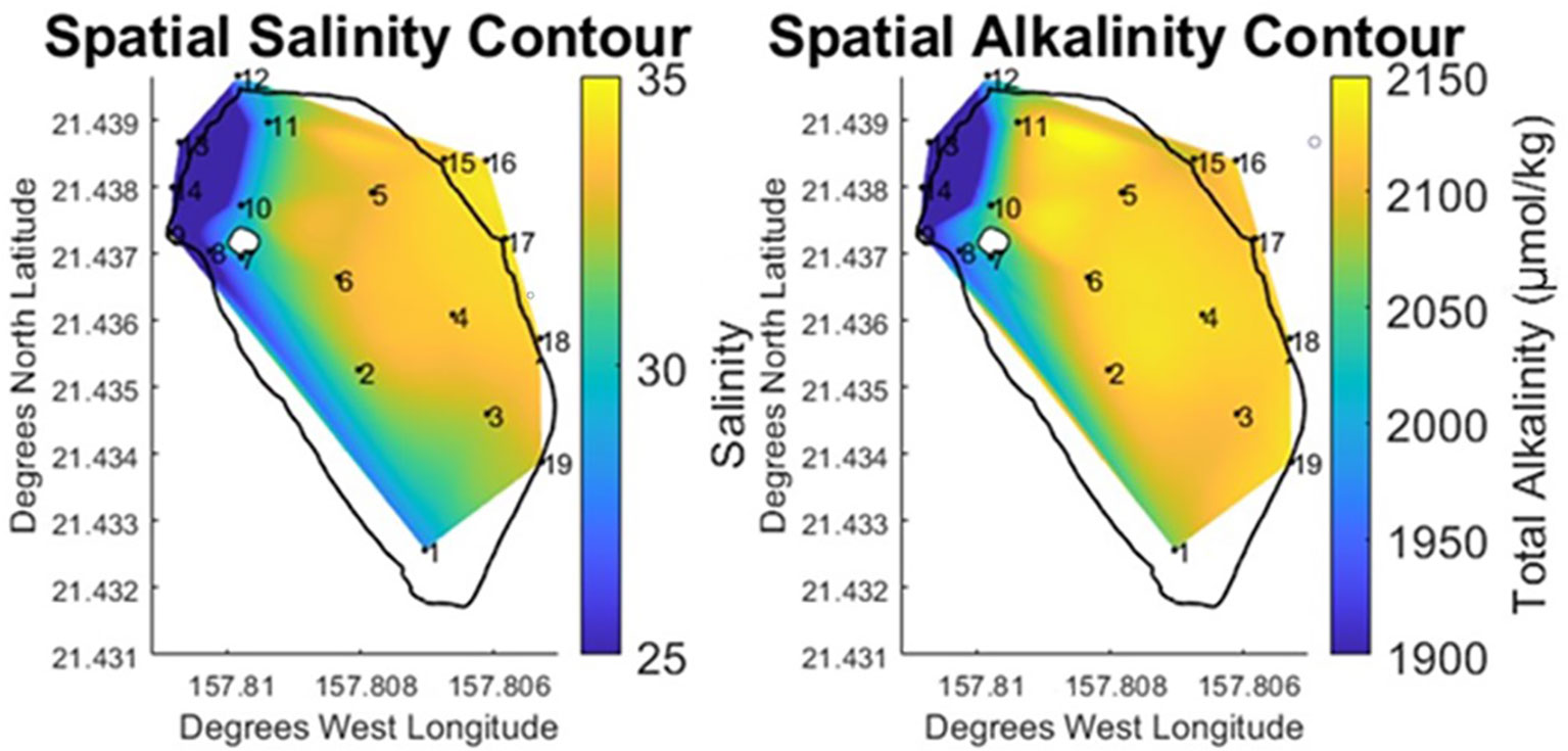
Figure 4 Vertically and temporally averaged contours of horizontal variability in Salinity and Total Alkalinity at He‘eia Fishpond during the study period. Stations IDs (numbered in black) are plotted on contour to show sampling locations.

Separate from the center pond zone were distinct north (stations 10 & 11) and south (stations 1 & 7-9) brackish zones. The brackish gradient observed in the north of the pond ran from the stream mākāhā at 13 towards the stream mouth mākāhā (12). Across this brackish gradient in the north, salinity decreased by 15% (-5.1) while TA fell by 6% (-81.1 μmol·kg⁻¹). A similar salinity mixing gradient ran south along the landward edge of the pond from the stream mākāhā at 13 towards station 1 at the south end of the pond. This southward oriented gradient exhibited a 24% decline in salinity (-8.1) and 9% in TA (-145.1 μmol·kg⁻¹). For these stations in the north and south brackish zones, the pattern observed in the salinity and alkalinity data (Figure 4) showed stream water entering the pond near station 9. From there the stream water exhibited traditional estuarine mixing, branching to the north and south around the former mangrove island.

Flow direction was not measured directly in this study. However, the two salinity gradients provide an indication of the direction of stream water flow within the pond. Using gradients in salinity as a proxy for water flow direction, provides further detail to distinguish between the brackish zones observed in the north and south of the pond. Due to the close proximity of the north zone to four mākāhā, brackish mixing occurred over a shorter spatial area, relative to the brackish mixing in the southward direction, which was spread out across the length of landward edge of the pond. While alkalinity was observed to be conservative with salinity throughout the pond, the large variability in salinity and TA observed in the south of the pond underscores a relative concentration of stream water in this area, due to its spatial isolation from mākāhā. The north of the pond exhibited the opposite behavior, where a smaller distance to multiple mākāhā was represented by a smaller variability in both salinity and TA. Therefore, proximity to the mākāhā water flux sites played a significant role in determining the magnitude of brackish mixing within the pond and the balance of stream and bay water contributions in the north and south of the pond.

While the north and south zones in the pond were relatively similar with respect to salinity and TA, these areas diverged more noticeably when examined using DIC & % O₂ data. The north end of the pond exhibited DIC concentrations similar to those measured at the ocean endmember (+3 μmol·kg⁻¹), while the % O₂ data were slightly lower (-10% O2 saturation). The south and center of the pond displayed a 4% elevation in DIC (+51 μmol·kg⁻¹) above what was observed at the ocean endmember. Likewise, the south and center of the pond exhibited a 30% drop in O₂ saturation relative to the bay. The spatial contour plots for these parameters (Figure 5) clearly shows a low oxygen, high DIC region starting at the south of the pond and expanding north through the pond center. Given what is known about the generalized path of brackish water circulation within the pond, this data suggests both a DIC source located in the south of the pond as well as a difference in the residence times between the north and south of the pond.

FIGURE 5

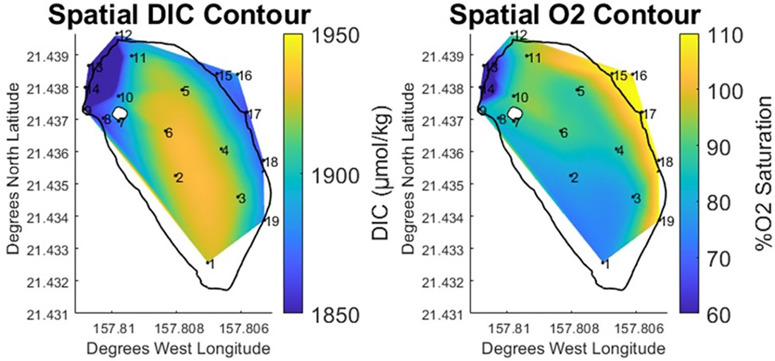
Figure 5 Vertically and temporally averaged contours of horizontal variability in % Oxygen Saturation and DIC at He‘eia Fishpond during the study period. Stations IDs (numbered in black) are plotted on contour to show sampling locations.

Water entering the pond through the bay-facing mākāhā was super saturated with oxygen due to the vigorous mixing that occurs while passing through the slotted sluices gates. As has been described, bay-water exerts the vast majority of control on pond composition. However, since sampling was conducted across neap ebb tides, it is reasonable to expect that O₂ super-saturated bay water will have minimal effect on measurements conducted within the pond. The data supports this assumption, as the mean %O₂ saturation measured at the mākāhā was 109%, while mean oxygen values in the pond were below 93%. DIC measurements were similarly consistent between the mākāhā (1874.0 μmol·kg⁻¹, 2σ=29.6). Measurements within the pond clearly demonstrated modification of oxygen and DIC parameters, particularly at the south of the pond. A signal of enhanced respiration was observed at station 1, where oxygen saturation fell to 73.67%, while DIC increased to 1923.8 μmol·kg⁻¹. This signal extends up through the center of the pond, where all of the stations (2-6) exhibit similarly high DIC, while oxygen slowly increases moving northward. Based on the known path of the brackish gradient running down the landward edge of the fishpond, and the relative abundance of organic matter found in stream water in comparison with bay-derived water, the likely cause of the observed respiration signal is the breakdown of stream-derived organic matter deposited at the south end of the pond (Alongi et al., 2004; Bouillon et al., 2008).

The observed pattern in respiration makes the north south difference more apparent. As stated, brackish waters to the north (stations 10 & 11) have compositions similar to those measured in the south (station 1), so it is likely that stream derived organic matter is present in the north end of the pond. As previously observed, primary difference between the north and south ends of the pond is their position relative to the location of stream and bay-facing mākāhā. The south end of the pond is at the far end of the brackish water gradient, fed by the freshwater stream mākāhā. This position is at the opposite end of the pond from both the bay-facing mākāhā and the stream mākāhā, with the result that water travels southward along the brackish gradient, before recirculating north through center of the pond, towards the bay-facing mākāhā. In comparison, the north end of the pond is located between the freshwater stream mākāhā, the bay-facing mākāhā, as well as the stream mākāhā at the mouth of He‘eia stream (12). This likely means that the north end of the pond is flushing more completely and with higher frequency than the south end of the pond. The consequent difference in residence time would support the observed difference in DIC and oxygen measurements between the north and south zones in the pond, as the breakdown of organic matter is likely occurring at both locations, but the shorter residence time at the north end of the pond prevents the respiration signal from manifesting as significantly as it does in the south end of the pond.

Comparing these results with other carbon parameters measured (Figure 3), it does not appear that TA, pH, and Ω_Ar exhibit the same north/south pattern observed in the DIC and O₂ saturation data. Whereas the DIC peak and O₂ saturation minima were located around station 1, the lowest measurements for TA, pH and Ω_Ar were all collocated at station 9, near the freshwater stream mākāhā. Given this spatial shift and the proximity to the stream, the observed variability in TA, pH, and Ω_Ar was more directly controlled by the balance between fresh and bay-water during brackish mixing rather than by in-situ biogeochemical processes.

The pCO₂ data (Figure 3G) shows that He‘eia was a net source of CO₂ during the study period. The annual mean atmospheric pCO₂ reported by the NOAA Mauna Loa Observatory in 2020 (414 μatm) was visualized alongside the pCO₂ data to better show sink/source behavior. Given that both He‘eia Stream and Kāne‘ohe Bay were observed to behave as CO₂ sources, it was expected that the stations within the pond would exhibit values between the two water sources for the pond. Furthermore, the station groups followed pattern in pCO₂ that mirrored the variability in salinity. The lower mean pCO₂ observed within the center of the pond (605.5 μatm) further underscores the connection to the mākāhā stations (477.7 μatm). Likewise, pCO₂ was observed to rise in both the north (845.0 μatm) and south (997.9 μatm) of the pond, as these more brackish regions of the pond were more heavily influenced by effect of the high pCO₂ values in He‘eia Stream (7994.1 μatm). While the stream values for pCO₂ were exceptionally high, the influence of stream waters on the pond were limited, as evidenced by the increases in pCO₂ observed in brackish regions in both the north and south of the pond. These north and south regions in the pond were still significant CO2 sources. However, the approximately 7000 μatm drop in mean pCO₂ suggests that the pond source behavior is more directly controlled by the sink/source behavior in Kāne‘ohe Bay (Fagan and Mackenzie, 2007; Massaro et al., 2012; Drupp et al., 2013). This is likely due to He‘eia Stream having a small spatial area and volume, as well as supplying a smaller volume of water to the pond relative what is supplied by Kāne‘ohe Bay.

5.2 Benthic respiration

Weak stratification has been observed at the fishpond in previous studies (Möhlenkamp et al., 2018). In order to better understand how any potential stratification would influence the carbon system during this project, samples were taken at surface and at depth at each station within the fishpond throughout the study period. Comparing the vertically averaged data (Figure 5) with the surface/depth data (Figure 6) it is clear that the previously described respiration signal is enhanced at depth. The contour of peak elevated DIC covers a wider spatial area at the south end of the pond. Likewise, the lower range of elevated DIC extends north along the landward edge of the pond towards stations 8 & 9. Previous studies documented benthic diatoms (Vasconcellos, 2007) and invasive benthic algae (Murphy, 2012) in the fishpond. Higher concentrations of chlorophyll-a were observed at stations along the landward edge of the pond and near the freshwater mākāhā.

FIGURE 6

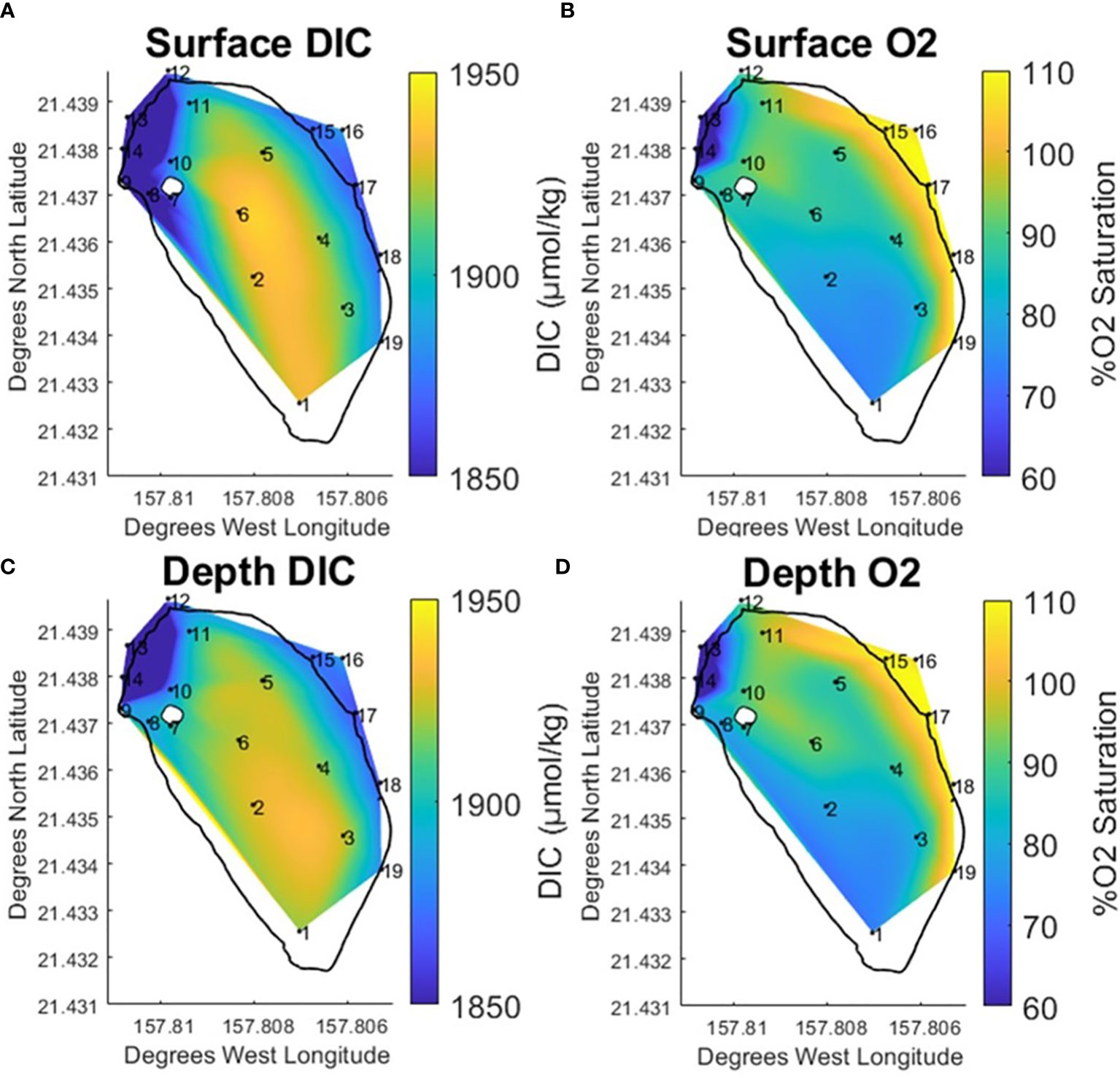
Figure 6 Temporally averaged contours for surface DIC (A) and % O2 Saturation (B) and Depth DIC (C) and % O2 Saturation (D) at He‘eia Fishpond during the study period. Stations IDs (numbered in black) are plotted on contour to show sampling locations.

Temperature and salinity data reveal clear differences in the potential for stratification between north and south regions along the landward edge of the pond. In the same southern space as the expanded peak DIC elevation at depth, the salinity data was observed to be vertically homogenous. Meanwhile, temperature increased by approximately 1 °C at depth. The temperature and salinity data would suggest that the south end of the pond is not significantly stratified. Likewise, assuming that the elevated temperature at depth is associated with biological activity in the sediments, the observed respiration signal is likely predominately derived from microbial breakdown of organic matter deposited in benthic sediments. This corroborates previous research examining sediment microbial oxygen consumption related to benthic algae (Murphy, 2012) and benthic organic matter remineralization (Briggs, 2011; Briggs et al., 2013a; Briggs et al., 2013b) within the fishpond. Both studies conducted diurnal experiments and documented sediment O₂ drawdown between sundown and sunrise, when respiration dominated over photosynthetic O₂ production, in bottom sediments.

The station 8 & 9 area to the north of the pond displayed a trend in salinity, which decreased significantly at the surface, opposite to that observed in the south. The decrease in salinity is likely due to the close proximity of the freshwater stream mākāhā. Meanwhile, a vertical temperature inversion was visible, similar to that described in the south of the pond. In this case, stratification seems likely as the salinity data shows a concentration of stream water input at the surface. Given this stratification, the temperature inversion in the north is better explained by the relatively cooler stream water remaining vertically confined at the surface.

Since stratification does not appear to be spatially uniform within the pond, it is unclear whether the benthic-derived respiration signal varies spatially within the pond. While neither microbial activity nor pore water chemistry were collected during this study, the ratio of TA and DIC can be used to examine the dominant biological processes interacting with the carbon system (Borges, 2003; Rixen et al., 2012; Sippo et al., 2016). TA and DIC are influenced by a number of biological processes in predictable ways. The dissolution of calcium carbonate produces TA and DIC at a ratio of 2:1. Likewise, aerobic respiration of organic matter reduces TA while increasing DIC at a ratio of 1:10 (Rixen et al., 2012; Sippo et al., 2016).

In order to understand how the balance of TA and DIC was driven at each of the in-pond stations, the TA and DIC measurements were normalized to endmember measurements to account for traditional estuarine mixing. For this experiment, traditional estuarine mixing was defined as the dilution of seawater with freshwater, resulting in a linear mixing gradient in salinity. The normalized values were then subtracted from the measured values to arrive at ΔTA and ΔDIC values capturing only the effects of in situ biogeochemical alteration. This data was plotted alongside surface and depth data for DIC and precent O₂ saturation (Figure 7) to examine the net biological activity at each station and depth within the fishpond. The arrows plotted over each point denote the slope of the curve fit to the ΔTA and ΔDIC data at that station and depth, with 1:1 slope line provided as a visual reference for an approximate balance between calcium carbonate dissolution and respiration.

FIGURE 7

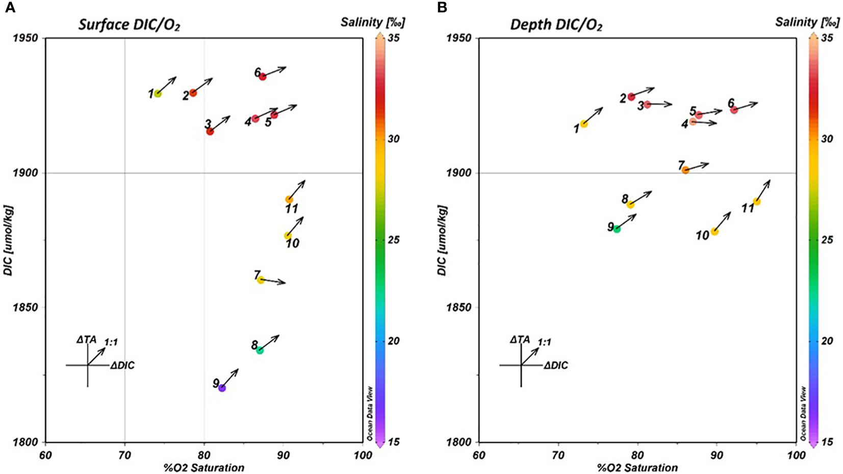
Figure 7 DIC-O2 Saturation plots for surface (A) and depth (B) measurements at the 11 in-pond sampling stations. The color bar indicates the mean salinity observed at each plotted station and depth. The arrows plotted from each point indicate the slope of the fitted curve of the ΔTA/ΔDIC relationship at that station and depth.

The DIC-O₂ data reveal that while the north and south ends of the pond remain largely unchanged between surface and depth measurements, there is a large shift in the DIC-O₂ relationship observed in the brackish water gradient (stations 7-9). A large increase in DIC was observed at depth at all three of the stations, in addition to a small decrease in O₂ saturation at stations 8 and 9. On account of the large shift in salinity between surface and depth at these stations, and the previously identified stratification, it is likely that this shift in DIC is driven by a difference in the balance of fresh and bay-derived water between surface and depth.

The water measured in He‘eia Stream was found to have a significantly lower concentration of DIC (1623.2 μmol·kg⁻¹) than the water from Kāne‘ohe Bay (1874.0 μmol·kg⁻¹). Therefore, given that stream water was observed to be concentrated in the stratified surface layer at stations 7-9, the observed variability in DIC at those stations is likely due to the increased proportion of stream-derived water in the surface layer.

The ΔTA/ΔDIC relationships (Arrows, Figures 7A, B) support an increased concentration of stream-derived water as the ΔTA/ΔDIC ratios at stations 8 & 9 do not significantly change between surface and depth. Similarly, the north end of the pond, stations 10 & 11, do not exhibit a change in the ΔTA/ΔDIC ratio between surface and depth, supporting the previous finding that the shorter residence time at the north end of the pond inhibits the biogeochemical alteration observed at stations in the south end of the pond. Likewise, the ΔTA/ΔDIC relationships show up clearly in the south and center pond stations (1-6) associated with the respiration signal. At each of these stations, the ΔTA/ΔDIC ratio decreases significantly with depth, indicating an increased influence of aerobic respiration.

6 Conclusion

Coastal and estuarine ecosystems are complex and highly dynamic. The carbon system has been historically understudied in these environments, and the spatial variability in carbon system parameters is thus poorly understood. The aim of this study was to constrain spatial variability in a model Hawaiian estuarine ecosystem. DIC and percent oxygen saturation were observed to vary significantly across the fishpond, as the distance from water flux locations and the direction of stream water flow controlled the magnitude of biogeochemical alteration of these parameters within pond. At the south end of the pond an enhanced respiration signal consisting of elevated DIC and undersaturated conditions with respect to oxygen was identified. Analysis of the biogeochemical effect on TA and DIC indicated that the enhanced respiration signal was more prevalent at depth. Prior studies observed higher concentrations of benthic algae in the organic matter rich sediments along the landward edge of the fishpond. The same benthic algae may be responsible for the respiration signal observed here. The comparison of this south pond pattern with other regions of the pond suggests significant differences in the mixing regimes and residence times, which may influence the distribution of nutrients and organic rich sediments that support benthic algae and other organisms. Future studies could build upon the observed patterns in carbon and oxygen by examining composition of benthic microbial communities and the distribution of macronutrients to better describe the drivers of this spatial variability. Likewise, additional carbon and oxygen work in He‘eia stream and Kāne‘ohe Bay would provide valuable context for how the management of this productive coastal space influences the broader estuarine environment.

Coastal managers working in the He‘eia estuarine space have encountered a range of challenges from anoxia and thermal stress events to wet season pulses of agro-ecological run off. Ten years of restoration work separate the benthic respiration signal observed here from previous studies documenting benthic algae and sediment oxygen consumption. While this restoration has improved water quality within the fishpond, it does not seem to have significantly altered benthic biological processes. The results here demonstrate a clear connection between how water sources mix within the fishpond and the spatial variability of carbon and oxygen. This data is a powerful tool for planning future management decisions within the estuary and the fishpond. The continued restoration work along the landward edge of He‘eia fishpond, the opening of additional mākāhā, and the enhancement of streamflow into the pond, would all likely reshape apparent residence times within the fishpond as well as the distribution of carbon and oxygen. In this way, understanding the drivers of spatial variability in carbon and oxygen better equips coastal communities to anticipate and respond to ecosystem change.

Data availability statement

The raw data supporting the conclusions of this article will be made available by the authors, without undue reservation.

Author contributions

All authors listed have made a substantial, direct, and intellectual contribution to the work and approved it for publication.

Acknowledgments

We would like to thank Hi‘ilei Kawelo and Kawika Winter who organized connections between researchers and community partners at the outset of this research. We are immensely grateful to groups working at Paepae o He‘eia, Kāko‘o ‘ŌIwi, and the He‘eia National Estuarine Research Reserve whose tireless ecosystem restoration work made this research possible. We would also like to thank Charles “Aka” Beebe and Rosie Alegado for their guidance during field preparation and site selection, as well as Paula Möhlenkamp for her assistance developing code in MATLAB. Likewise, we would like to thank Dan Sadler for his expertise and support while assembling the materials and equipment for conducting Winkler analyses. We are grateful to Kyle Conner, Lucie Knor, and Noah Howins for their technical and field support during this research. This research also benefited from the review and critique of Melissa Melendez and Nick Hawco, which helped improve the quality of this manuscript.

Funding

We acknowledge the financial support of our research provided in part by a grant/cooperative agreement from the National Oceanic and Atmospheric Administration, CMAR award # NA21NMF4320043. The views expressed herein are those of the author(s) and do not necessarily reflect the views of NOAA or any of its subagencies. This is SOEST contribution number 11610.

Conflict of interest

The authors declare that the research was conducted in the absence of any commercial or financial relationships that could be construed as a potential conflict of interest.

Publisher’s note

All claims expressed in this article are solely those of the authors and do not necessarily represent those of their affiliated organizations, or those of the publisher, the editors and the reviewers. Any product that may be evaluated in this article, or claim that may be made by its manufacturer, is not guaranteed or endorsed by the publisher.

References

Alongi D. M., Sasekumar A., Chong V. C., Pfitzner J., Trott L. A., Tirendi F., et al. (2004). Sediment accumulation and organic material flux in a managed mangrove ecosystem: Estimates of land–ocean–atmosphere exchange in peninsular Malaysia. Mar. Geology 208, 383–402. doi: 10.1016/j.margeo.2004.04.016

CrossRef Full Text | Google Scholar

Andersson A. J. (2005). Coastal ocean and carbonate systems in the high CO2 world of the anthropocene. Am. J. Sci. 305, 875–918. doi: 10.2475/ajs.305.9.875

CrossRef Full Text | Google Scholar

Bacastow R. D., Keeling C. D. (1973). “Atmospheric carbon dioxide and radiocarbon in the natural carbon cycle: II. changes form A.D. 1700 to 2070 as deduced from a geochemical model,” in Carbon in the biosphere. Eds. Woodwell G. M., Pecan E. V. (Washington, D.C.:U.S. A.E.C.,), 86–135.

Google Scholar

Bednaršek N., Harvey C. J., Kaplan I., Feely R. (2016). Pteropods on the edge: Cumulative effects of ocean acidification, warming, and deoxygenation. Prog. Oceanography 145 (2):1–24. doi: 10.1016/j.pocean.2016.04.002

CrossRef Full Text | Google Scholar

Benson B. B., Krause D. J. R. (1980). The concentration and isotopic fractionation of gases dissolved in freshwater in equilibrium with the atmosphere. 1. oxygen. Limnology Oceanography 25 (4), 662–671. doi: 10.4319/lo.1980.25.4.0662

CrossRef Full Text | Google Scholar

Benson B. B., Krause D. J. R. (1984). The concentration and isotopic fractionation of oxygen dissolved in freshwater and seawater in equilibrium with the atmosphere. Limnology Oceanography 29 (3), 620–632. doi: 10.4319/lo.1984.29.3.0620

CrossRef Full Text | Google Scholar

Borges A. V. (2003). Atmospheric CO ₂ flux from mangrove surrounding waters. Geophys. Res. Lett. 30, 1558. doi: 10.1029/2003GL017143

CrossRef Full Text | Google Scholar

Bouillon S., Borges A. V., Castañeda-Moya E., Diele K., Dittmar T., Duke N. C., et al. (2008). Mangrove production and carbon sinks: A revision of global budget estimates: Global mangrove carbon budgets. Global Biogeochem. Cycles 22, n/a–n/a. doi: 10.1029/2007GB003052

CrossRef Full Text | Google Scholar

Breitburg D., Levin L. A., Oschlies A., Grégoire M., Chavez F. P., Conley D. J., et al. (2018). Declining oxygen in the global ocean and coastal waters. Science 359, eaam7240. doi: 10.1126/science.aam7240

PubMed Abstract | CrossRef Full Text | Google Scholar

Bremer L., Falinski K., Ching C., Wada C., Burnett K., Kukea-Shultz K., et al. (2018). Biocultural restoration of traditional agriculture: Cultural, environmental, and economic outcomes of lo‘i kalo restoration in he‘eia, OA’hu. Sustainability 10, 4502. doi: 10.3390/su10124502

CrossRef Full Text | Google Scholar

Briggs R.A 2011 Organic Matter Remineralization in Coastal Sediments in and around Kaneohe Bay, Hawaii. University of Hawaii

Google Scholar

Briggs R. A., Padilla-Gamiño J. L., Bidigare R. R., Gates R. D., Ruttenberg K. C. (2013a). Impact of coral spawning on the biogeochemistry of a Hawaiian reef. Estuarine Coast. Shelf Sci. 134, 57–68. doi: 10.1016/j.ecss.2013.09.013

CrossRef Full Text | Google Scholar

Briggs R. A., Ruttenberg K. C., Glazer B. T., Ricardo A. E. (2013b). Constraining sources of organic matter to tropical coastal sediments: Consideration of nontraditional end-members. Aquat Geochem 19, 543–563. doi: 10.1007/s10498-013-9219-2

CrossRef Full Text | Google Scholar

Brix H., Gruber N., Keeling C. D. (2004). Interannual variability of the upper ocean carbon cycle at station ALOHA near Hawaii: Interannual variability at station ALOHA. Global Biogeochem. Cycles 18. doi: 10.1029/2004GB002245

CrossRef Full Text | Google Scholar

Cai W., Wang Y. (1998). The chemistry, fluxes, and sources of carbon dioxide in the estuarine waters of the satilla and altamaha rivers, Georgia. Limnology Oceanography 4, 657–668. doi: 10.4319/lo.1998.43.4.0657

CrossRef Full Text | Google Scholar

Caldeira K., Wickett M. E. (2003). Anthropogenic carbon and ocean pH. Nature 425, 365–365. doi: 10.1038/425365a

PubMed Abstract | CrossRef Full Text | Google Scholar

Camvel D. (2020). Ho‘oulu ‘Āina: Restoration in the he‘eia ahupua‘a (Honolulu, HI:University of Hawaii).

Google Scholar

Cao L., Zhang H., Zhang M., Wang S. (2014). Response of ocean acidification to a gradual increase and decrease of atmospheric CO2. Environ. Res. Lett. 9 (2). doi: 10.1088/1748-9326/9/2/024012

CrossRef Full Text | Google Scholar

Carpenter H. J. (1965). The Accuracy of the Winkler Method for Dissolved Oxygen Analysis. Limnology and Oceanography. 10, 1. doi: 10.4319/LO.1965.10.1.0135

CrossRef Full Text | Google Scholar

Chan F., Barth J. A., Blanchette C. A., Byrne R. H. (2017). Persistent spatial structuring of coastal ocean acidification in the California current system. Sci. Rep. 7, (1). doi: 10.1038/s41598-017-02777-y

PubMed Abstract | CrossRef Full Text | Google Scholar

Codispoti L. (2001). One man’s advice on the determination of dissolved oxygen in seawater 23.

Google Scholar

Costa-Pierce B. A. (1987). Aquaculture in ancient Hawaii. BioScience 37, 320–331. doi: 10.2307/1310688

CrossRef Full Text | Google Scholar

D’Andrea B. (2015). Water exchange and circulation in he‘eia fishpond: Building blocks for establishing a water budget (Honolulu, HI:University of Hawaii).

Google Scholar

De Carlo E., Hoover D., Young C., Hoover R., Mackenzie F. (2007). Impact of storm runoff from tropical watersheds on coastal water quality and productivity. Appl. Geochemistry 22, 1777–1797. doi: 10.1016/j.apgeochem.2007.03.034

CrossRef Full Text | Google Scholar

Demopoulos A. W. J., Fry B., Smith C. R. (2007). Food web structure in exotic and native mangroves: a Hawaii–Puerto Rico comparison. Oecologia 153, 675–686. doi: 10.1007/s00442-007-0751-x

PubMed Abstract | CrossRef Full Text | Google Scholar

Dickson A. (2001). Reference materials for oceanic CO₂ measurements. Oceanography (Washington D.C.) 14, 21–22.

Google Scholar

Dickson A. G., Sabine C. L., Christian J. R. (Eds) (2007). Guide to best practices for ocean CO2 measurements. PICES Special Publicationn 3, 191 pp.

Google Scholar

Doney S. C., Busch D. S., Cooley S. R., Kroeker K. J. (2020). The impacts of ocean acidification on marine ecosystems and reliant human communities. Annu. Rev. Environ. Resour. 45, 11.1–11.30. doi: 10.1146/annurev-environ-012320-083019

CrossRef Full Text | Google Scholar

Dore J. E., Lukas R., Sadler D. W., Church M. J., Karl D. M. (2009). Physical and biogeochemical modulation of ocean acidification in the central north pacific. Proc. Natl. Acad. Sci. 106, 12235–12240. doi: 10.1073/pnas.0906044106

CrossRef Full Text | Google Scholar

Drupp P., De Carlo E. H., Mackenzie F. T. (2016). Porewater CO2-carbonic acid geochemistry in sandy sediments. Mar. Chem. 185, 48–64. doi: 10.1016/j.marchem.2016.04.004

CrossRef Full Text | Google Scholar

Drupp P., De Carlo E. H., Mackenzie F. T., Bienfang P., Sabine C. L. (2011). Nutrient inputs, phytoplankton response, and CO2 variations in a semi-enclosed subtropical embayment, kaneohe bay, Hawaii. Aquat Geochem 17, 473–498. doi: 10.1007/s10498-010-9115-y

CrossRef Full Text | Google Scholar

Drupp P., De Carlo E. H., Mackenzie F. T., Sabine C. L. (2013). A comparison of CO2 dynamics and air-Sea exchange in differing tropical reef environments. Aquat. Geochemistry 19, 371–397. doi: 10.1007/s10498-013-9214-7

CrossRef Full Text | Google Scholar

Dulai H., Kleven A., Ruttenberg K., Briggs R., Thomas F. (2016). “Evaluation of submarine groundwater discharge as a coastal nutrient source and its role in coastal groundwater quality and quantity,” in Emerging issues in groundwater resources. Ed. Fares A. (Cham: Springer International Publishing), 187–221. doi: 10.1007/978-3-319-32008-3_8

CrossRef Full Text | Google Scholar

Fagan K. E., Mackenzie F. T. (2007). Air–sea CO2 exchange in a subtropical estuarine-coral reef system, kaneohe bay, Oahu, Hawaii. Mar. Chem. 106, 174–191. doi: 10.1016/j.marchem.2007.01.016

CrossRef Full Text | Google Scholar

Feely R., Okazaki R. R., Cai W., Bednaršek N. (2017). The combined effects of acidification and hypoxia on pH and aragonite saturation in the coastal waters of the California current ecosystem and the northern gulf of Mexico. Continental Shelf Res. 152, (2). doi: 10.1016/j.csr.2017.11.002

CrossRef Full Text | Google Scholar

Flynn K. J., Clark D. R., Mitra A., Fabian H. (2015). Ocean acidification with (de)eutrophication will alter future phytoplankton growth and succession. Proc. R. Soc. B: Biol. Sci. 282 (1804). doi: 10.1098/rspb.2014.2604

CrossRef Full Text | Google Scholar

Goodwin P., Lauderdale J. M. (2013). Carbonate ion concentrations, ocean carbon storage, and atmospheric CO2. Global Biogeochemical Cycles 27 (3), 882–893. doi: 10.1002/gbc.20078

CrossRef Full Text | Google Scholar

Hall E. R., Wickes L. N., Burnett L. E., Scott G. I. (2020). Acidification in the U.S. southeast: Causes, potential consequences and the role of the southeast ocean and coastal acidification network. Front. Mar. Sci. 7. doi: 10.3389/fmars.2020.00548

CrossRef Full Text | Google Scholar

Jokiel P. L., Rodgers K. S., Walsh W. J., Polhemus D. A., Wilhelm T. A. (2011). Marine resource management in the Hawaiian archipelago: The traditional Hawaiian system in relation to the Western approach. J. Mar. Biol. 2011, 1–16. doi: 10.1155/2011/151682

CrossRef Full Text | Google Scholar

Keala G., Hollyer J. R., Castro L. (2007). Loko i‘a: a manual on Hawaiian fishpond restoration and management (Honolulu: College of Tropical Agriculture and Human Resources, University of Hawai‘i at Mānoa).

Google Scholar

Kikuchi W. K. (1976). Prehistoric Hawaiian fishponds. Science 193 (4250), 295–299. doi: 10.1126/science.193.4250.295

PubMed Abstract | CrossRef Full Text | Google Scholar

Kleven A. (2014). Coastal groundwater discharge as a source of nutrients to heeia fishpond, Oahu, HI (Honolulu, HI:University of Hawaii).

Google Scholar

Knor L., Meléndez M., Howins. N., Boeman D., Lechner E., De Carlo E., et al. (2018). Dissolved inorganic carbon, total alkalinity, water temperature and salinity collected from surface discrete observations using coulometer, alkalinity titrator and other instruments from the coral reef MPCO2 buoys at ala wai, CRIMP-2, kaneohe, and kilo nalu from 2016-01-08 to 2020-12-20 (NCEI accession 0176671). NOAA Natl. Centers Environ. Information doi: 10.25921/pe6v-qg74

CrossRef Full Text | Google Scholar

Koshiba S., Besebes M., Soaladaob K., Isechal A. L., Victor S., Golbuu Y. (2013). Palau’s taro fields and mangroves protect the coral reefs by trapping eroded fine sediment. Wetlands Ecol. Manage 21, 157–164. doi: 10.1007/s11273-013-9288-4

CrossRef Full Text | Google Scholar

Laurent A., Fennel K., Cai W., Huang W., Barbero L., Wanninkhof R. (2017). Eutrophication-induced acidification of coastal waters in the northern gulf of Mexico: Insights into origin and processes from a coupled physical-biogeochemical model: Acidification in NGOM eutrophic waters. Geophysical Res. Lett. 44 (2), 946–956. doi: 10.1002/2016GL071881

CrossRef Full Text | Google Scholar

Leon Soon S. (2017). Biophysical interactions: Influence of water flow on nutrient distribution and nitrate uptake by marine algae. [Dissertation/PhD Thesis]. (Honolulu, HI:University of Hawaii)

Google Scholar

Lopera D. (2020). Understanding change: Examining the effect of ahupua‘a restoration efforts on water circulation in loko i‘a o he‘eia, a native Hawaiian fishpond (Honolulu, HI:University of Hawaii).

Google Scholar

Maly K., Maly O. (2003). Ka hana lawai‘a a me nā ko‘a o na kai ‘ewalu : a history of fishing practices and marine fisheries of the Hawaiian islands (Keeau, HI:Kumu Pono Associates).

Google Scholar

Massaro R. F. S., De Carlo E. H., Drupp P. S., Mackenzie F. T., Jones S. M., Shamberger K. E., et al. (2012). Multiple factors driving variability of CO2 exchange between the ocean and atmosphere in a tropical coral reef environment. Aquat Geochem 18, 357–386. doi: 10.1007/s10498-012-9170-7

CrossRef Full Text | Google Scholar

McCoy D., McManus M. A., Kotubetey K., Kawelo A. H., Young C., D’Andrea B., et al. (2017). Large-Scale climatic effects on traditional Hawaiian fishpond aquaculture. PloS One 12, e0187951. doi: 10.1371/journal.pone.0187951

PubMed Abstract | CrossRef Full Text | Google Scholar

Möhlenkamp P., Beebe C., McManus M., Kawelo A., Kotubetey K., Lopez Guzman M., et al. (2019). Kū hou kuapā: Cultural restoration improves water budget and water quality dynamics in he‘eia fishpond. Sustainability 11, 161. doi: 10.3390/su11010161

CrossRef Full Text | Google Scholar

Murphy J. L. (2012). Linking Benthic Algae to Sediment Oxidation-Reduction Dynamics: Implications for Sediment-Water Interface Nutrient Cycling. [Dissertation/PhD Thesis]. [Honolulu (HI)]: University of Hawaii

Google Scholar

Ono H., Kosugi N., Toyama K., Tsujino H. (2019). Acceleration of ocean acidification in the Western north pacific. Geophysical Res. Lett. 46 (22), 13161–13169. doi: 10.1029/2019GL085121

CrossRef Full Text | Google Scholar

Orr J. C., Fabry V. J., Aumont O., Bopp L., Doney S. C., Feely R. A., et al. (2005). Anthropogenic ocean acidification over the twenty-first century and its impact on calcifying organisms. Nature 437, 681–686. doi: 10.1038/nature04095

PubMed Abstract | CrossRef Full Text | Google Scholar

Pierrot D. E., Lewis E., Wallace D. W. R. (2006). MS excel program developed for CO2 system calculations (Oak Ridge, Tennessee: Carbon Dioxide Information Analysis Center, Oak Ridge National Laboratory, U.S. Department of Energy). doi: 10.3334/CDIAC/otg.CO2SYS_XLS_CDIAC105a

CrossRef Full Text | Google Scholar

Riebesell U., Zondervan I., Rost B., et al. (2000). Reduced calcification of marine plankton in response to increased atmospheric CO2. Nature 407, 364–367. doi: 10.1038/35030078

PubMed Abstract | CrossRef Full Text | Google Scholar

Ringuet S., Mackenzie F. (2005). Controls on nutrient and phytoplankton dynamics during normal flow and storm runoff conditions, southern kaneohe bay, Hawaii. Estuaries 28, 327–337. doi: 10.1007/BF02693916

CrossRef Full Text | Google Scholar

Rixen T., Jiménez C., Cortés J. (2012). Impact of upwelling events on the sea water carbonate chemistry and dissolved oxygen concentration in the Gulf of Papagayo (Culebra Bay), Costa Rica: Implications for coral reef. Revista de Biologia Tropical 60, 6 187. doi: 10.15517/rbt.v60i2.20004

PubMed Abstract | CrossRef Full Text | Google Scholar

Rixen T., Jiménez C., Cortés J. (2015). Impact of upwelling events on the sea water carbonate chemistry and dissolved oxygen concentration in the gulf of papagayo (Culebra bay), Costa Rica: Implications for coral reefs. Revista de Biologia Tropical 60, 187. doi: 10.15517/rbt.v60i2.20004

CrossRef Full Text | Google Scholar

Rodgers K. S., Jokiel P. L., Western Weather Group, Inc (2005). HIMB weather station: Moku o loe (Coconut island), Oahu, Hawaii (Honolulu, HI:Pacific Islands Ocean Observing System). Available at: http://pacioos.org/metadata/AWS-HIMB.html.

Google Scholar

Shamberger K. E. F., Feely R. A., Sabine C. L., Atkinson M. J., DeCarlo E. H., Mackenzie F. T., et al. (2011). Calcification and organic production on a Hawaiian coral reef. Mar. Chem. 127, 64–75. doi: 10.1016/j.marchem.2011.08.003

CrossRef Full Text | Google Scholar

Sippo J. Z., Maher D. T., Tait D. R., Holloway C., Santos I. R. (2016). Are mangroves drivers or buffers of coastal acidification? insights from alkalinity and dissolved inorganic carbon export estimates across a latitudinal transect. Global Biogeochem. Cycles 30, 753–766. doi: 10.1002/2015GB005324

CrossRef Full Text | Google Scholar

University of Hawaii Sea Grant (2018) Kingtide. Available at: https://seagrant.soest.hawaii.edu/coastal-and-climate-science-and-resilience/ccs-projects/what-is-a-king-tide (Accessed August 25, 2022).

Google Scholar

U.S. Geological Survey (2011) Change to solubility equations for oxygen in water: Office of water quality technical memorandum (Accessed July 15, 2011).

Google Scholar

U.S. Geological Survey (2016) National water information system data available on the world wide web (USGS water data for the nation). Available at: https://waterdata.usgs.gov/usa/nwis/uv?16275000 (Accessed August 25, 2022).

Google Scholar

Vasconcellos S. (2007). Distribution and characteristics of a photosynthetic benthic microbial community in a marine coastal pond, Vol. 25. Pacific Internship Programs for Exploring Sciences (PIPES) Final Report (Hilo, Hawaii:University of Hawaii).

Google Scholar

Winter K., Beamer K., Vaughan M., Friedlander A., Kido M., Whitehead A., et al. (2018). The moku system: Managing biocultural resources for abundance within social-ecological regions in hawai‘i. Sustainability 10, 3554. doi: 10.3390/su10103554

CrossRef Full Text | Google Scholar

Winter K. B., Lincoln N. K., Berkes F., Alegado R. A., Kurashima N., Frank K. L., et al. (2020a). Ecomimicry in indigenous resource management: optimizing ecosystem services to achieve resource abundance, with examples from hawai‘i. E&S 25, art26. doi: 10.5751/ES-11539-250226

CrossRef Full Text | Google Scholar

Winter K. B., Rii Y. M., Reppun F. A. W. L., Hintzen K. D., Alegado R. A., Bowen B. W., et al. (2020b). Collaborative research to inform adaptive comanagement: a framework for the he‘eia national estuarine research reserve. E&S 25, art15. doi: 10.5751/ES-11895-250415

CrossRef Full Text | Google Scholar

Wong G. T. F. (2012). Removal of nitrite interference in the winkler determination of dissolved oxygen in seawater. Mar. Chem. 130, 28–32. doi: 10.1016/j.marchem.2011.11.003

CrossRef Full Text | Google Scholar

Yang L. (2000). A circulation study of Hawaiian fishponds; university of Hawaii (Department of Ocean and Resources Engineering: Honolulu, HI).

Google Scholar

Young C. W. (2011). Perturbation of nutrient level inventories and phytoplankton community composition during storm events in a tropical coastal system: Heeia fishpond (Honolulu HI: University of Hawaii).

Google Scholar